A note on the distribution of admixture segment lengths and ancestry proportions under pulse and two-wave admixture models

Present-day genomes are mosaics of ancestries from the different sources that merged to form modern populations (e.g., Price et al. (2009); Brisbin et al. (2012); Maples et al. (2013)). Estimating the time of each admixture event and the relative contribution of each source population is an important problem in population genetics. To estimate admixture times, Johnson et al. (2011) fitted the number of ancestry switches; Pugach et al. (2011), and later Sanderson et al. (2015), matched simulations to the typical segment length, as estimated from a wavelet transform of the local ancestry along the genome; and Pool and Nielsen (2009), as well as Gravel (2012), fitted the distribution of segment lengths. However, these methods require an accurate identification of the boundaries of admixture segments, which is not always available, in particular for computationally phased data. Reich and colleagues (Moorjani et al., 2011; Patterson et al., 2012; Loh et al., 2013; Pickrell et al., 2014) fitted the decay of admixture linkage disequilibrium (LD) with genetic distance, but such methods can be confounded by background LD. Hellenthal et al. (2014) recently proposed a promising approach based on the probability of two fixed loci to have given ancestries. Gene flow parameters can also be inferred using more general demographic inference methods, e.g., based on the allele frequency spectrum (Excoffier et al., 2013; Gutenkunst et al., 2009) or segment sharing (Palamara and Pe’er, 2013); however, to use these methods one must specify and infer a model for the entire history.

Recently, Rosenberg and colleagues (Verdu and Rosenberg, 2011; Goldberg et al., 2014; Goldberg and Rosenberg, 2015), Liang and Nielsen (2014a), and Gravel (2012) derived analytical results for the moments of the ancestry proportion, namely, the fraction of a chromosome that descend from a given source population. These ancestry proportions can be reliably inferred (e.g., Alexander et al. (2009); Pritchard et al. (2000)), and the derived moments have been used for admixture time inference (e.g., Botigué et al. (2013); Liang and Nielsen (2014b); Moreno-Mayar et al. (2014)). However, these methods did not make use of the entire distribution, as no analytical results were available. Here, we derive first results for the distribution of the ancestry proportions. We obtain an explicit formula for the case of a “pulse” admixture event, and we demonstrate its application to the inference of the admixture parameters. We then derive an expression in Laplace space for a general admixture model of arbitrary complexity, but which requires knowledge of the distribution of admixture segment lengths. For the special case of a “two-wave” admixture, we obtained the segment length distribution, and consequently, through numerical Laplace inversion, the distribution of ancestry proportions.

Consider the pulse model, where an admixed population formed $t$ generations ago as a result of merging of populations A and B, and where the proportions of ancestry contributed by A and B were $m$ and $1-m$, respectively. Under this model, each locus in a chromosome of a present-day admixed individual can trace its origin to A or B with probabilities $m$ and $1-m$, respectively. We assume lineages break apart along the chromosome, due to recombination, at rate $t$ per Morgan. Ignoring genetic drift and the underlying pedigree, we assume that upon recombination, the new source population is selected at random. Therefore, a recombination event will lead to a change of ancestry from A to B with probability $1-m$ and from B to A with probability $m$. The lengths chromosomal segments with A ancestry will thus be exponentially distributed with rate $(1-m)t$, and similarly for the B segments (rate $mt$) (Gravel, 2012). We neglect the first generation after admixture, where A and B segments do not yet mix (Gravel, 2012). As pointed out by Liang and Nielsen (2014a), the assumption of independent and exponentially distributed segment lengths breaks down for very short and very long times since admixture, due to the effect of the underlying pedigree and the accumulation of genetic drift, respectively. Nevertheless, for the relevant time-scales and effective population sizes of many human populations (around 10-200 generations and effective size in the thousands), segment lengths should be extremely well approximated by independent exponentials.

Given a chromosome of length $L$ (Morgans), the ancestry along the chromosome can be modeled as a two-state process with states A and B, and with the distribution of segment lengths in each state given above. We are interested in the distribution of $x$, the fraction of the chromosome in state A. Adopting a result of Stam (1980), the desired distribution is given by

	$\displaystyle f(x;L)$	$\displaystyle=(1-m)e^{-mh}\delta(x)+me^{-(1-m)h}\delta(1-x)$		(1)
		$\displaystyle+m(1-m)he^{-h\left[(1-m)x+m(1-x)\right]}\times$
		$\displaystyle\qquad\qquad\times\left\{\frac{mx+(1-m)(1-x)}{\alpha}I_{1}(2h\alpha)+2I_{0}(2h\alpha)\right\},$

where $h\equiv tL$, $\alpha\equiv\sqrt{m(1-m)x(1-x)}$, and $I_{0}$ and $I_{1}$ are the modified Bessel functions of the first kind of order 0 and 1, respectively. Note the delta functions at $x=0$ and $x=1$, corresponding to the probability of the entire chromosome having B only or A only ancestry, respectively. The mean ancestry proportion satisfies $\left\langle x\right\rangle=m$, as expected. The variance is given by

$${\rm Var}\,[x]=\frac{2m(1-m)}{h^{2}}\left(e^{-h}+h-1\right),$$

(2)

in agreement with Eq. (A16) in Gravel (2012). Note that Eq. (1) represents the distribution of the ancestry proportion across repetitions of the ancestral process (for a single chromosome), rather than across chromosomes from a sample (Gravel, 2012; Liang and Nielsen, 2014b). However, unless the population is very small (compared to the admixture time and the sample size), histories of different chromosomes are to a good approximation independent, and the two distributions are the same.

In theory, given the observed ancestry proportion for each chromosome in a sample, Eq. (1) can be used to compute the likelihood of the observed data for given admixture parameters. In practice, in the absence of trios or pedigree information, phase switches are abundant, and hence, it is difficult to accurately determine the ancestry proportion per chromosome. However, it is still possible to determine the diploid ancestry proportion, $y=(x_{1}+x_{2})/2$. Given that homologous chromosomes have independent histories, the diploid ancestry proportion distribution, $f_{d}(y;L)$, can be computed from Eq. (1) by convolution. Suppose we are now given the diploid ancestry proportions $y_{ij}$ for individuals $i=1,...,n$ and for chromosomes $j=1,...,22$ (where each chromosome has length $L_{j}$). Assuming chromosomes are independent both within and between individuals, the likelihood of the data is given by

$$\textrm{likelihood}=\prod_{i=1}^{n}\prod_{j=1}^{22}f(y_{ij};L_{j})$$

(3)

Maximum likelihood estimates (MLE) for $m$ and $t$ can then be obtained by a simple grid search. Simulation results with perfect knowledge of segment boundaries demonstrated that the method can infer correctly both $m$ and $t$ (Figure 1), although the variance increases with $t$, as expected. Coalescent simulations followed by inference of ancestry proportions using ADMIXTURE (Alexander et al., 2009) and application of our method demonstrated again high accuracy, at least as long as the A and B population were sufficiently diverged (not shown). However, when A and B are closely related, the distributions of the true and inferred ancestry proportions may differ, affecting the accuracy of the method.

We have so far considered a simple pulse model, under which the distributions of segment lengths are exponential with known rates. Under a more complex admixture history, we assume that the distributions of the lengths of A and B segments take the general form $q_{\textbf{A}}(\ell)$ and $q_{\textbf{B}}(\ell)$. We still assume that A and B segments are independent (see below). The process can then be modeled as a two-state process. We start on the left end of the chromosome in state A or B with probabilities $p_{A}=\left\langle\ell_{A}\right\rangle/\left(\left\langle\ell_{A}\right\rangle+\left\langle\ell_{B}\right\rangle\right)$ and $1-p_{A}$, respectively (where $\left\langle\ell_{A}\right\rangle$ and $\left\langle\ell_{B}\right\rangle$ are the mean segment lengths), and draw a random segment length from the selected ancestry. When the first segment terminates, we switch ancestries and draw a segment length from the other ancestry, and so on until we reach the end of the chromosome.

The distribution of $x$, the A ancestry proportion, can be computed in Laplace space by extending renewal theory methods developed in the physics domain (e.g., Godrèche and Luck (2001); Margolin and Barkai (2004)). Let $s$ be the Laplace pair of $L$ (the total chromosome length) and $u$ as the Laplace pair of $L_{A}\equiv xL$ (the total chromosome length covered by $A$ segments). We transform the density $f(L_{A};L)$ (from which the density of $x$ can be easily obtained) to $\hat{f}(u;s)$, and after some calculations, we obtain

$$\hat{f}(u;s)=\frac{s\left[1-\hat{q}_{\textbf{A}}(s+u)\hat{q}_{\textbf{B}}(s)\right]+u\left[1-\hat{q}_{\textbf{B}}(s)\right]\left\{1-p_{A}\left[1-\hat{q}_{\textbf{A}}(s+u)\right]\right\}}{s(s+u)\left[1-\hat{q}_{\textbf{A}}(s+u)\hat{q}_{\textbf{B}}(s)\right]}.$$

(4)

In the above equation, $\hat{q}_{\textbf{A}}(s)$ and $\hat{q}_{\textbf{B}}(s)$ are the Laplace transforms ($\ell\rightarrow s$) of $q_{\textbf{A}}(\ell)$ and $q_{\textbf{B}}(\ell)$, respectively. The details of the derivation are somewhat tedious and therefore omitted. It can be shown, using Eq. (4), that the mean ancestry proportion $\left\langle x\right\rangle$ approaches $p_{A}$ as $L\rightarrow\infty$. It can be also shown that Eq. (4) reduces to Eq. (1) for the admixture pulse model.

To obtain concrete results for complex admixture histories, we use the model developed by Gravel (2012) (section General incoming migration in the absence of drift and Figure 3 there). Gravel proposed that the ancestry along the chromosome could be described by a Markov process, whose states correspond to the identity of the source population (i.e., A or B), combined with the time when each segment entered the admixed population. Gravel then derived the transition rates for any admixture history. While the extended state space process is Markovian under any history, consecutive A and B segment lengths are generally no longer independent. However, little thought reveals that as long as migration beyond the the initial event is limited to one population, consecutive segment lengths remain independent.

Consider a model where populations A and B have merged $t_{1}$ generations ago, contributing proportions $m$ and $1-m$ to the admixed population. Then, $t_{2}$ ($<t_{1}$) generations ago, migrants from population A have replaced a proportion $\mu$ of the gene pool of the admixed population. No other events then take place until the present. The corresponding Markov process, using the method of Gravel (2012), has three states: $A_{1}$, $A_{2}$, and $B$, representing migrant segments from A at time $t_{1}$, from A at time $t_{2}$, and from B (at time $t_{1}$), respectively. Let us compute the distributions of the lengths of A and B segments.

The transition rate is $t_{1}$ when at states $A_{1}$ and $B$, and $t_{2}$ when at $A_{2}$. It can be shown that once a transition is made, the next state is chosen according to the following transition probability matrix

$$\mathbf{P}=\left(\begin{matrix}m\left(1-\mu\frac{t_{2}}{t_{1}}\right)&\mu\frac{t_{2}}{t_{1}}&(1-m)\left(1-\mu\frac{t_{2}}{t_{1}}\right)\\ m(1-\mu)&\mu&(1-m)(1-\mu)\\ m\left(1-\mu\frac{t_{2}}{t_{1}}\right)&\mu\frac{t_{2}}{t_{1}}&(1-m)\left(1-\mu\frac{t_{2}}{t_{1}}\right)\end{matrix}\right).$$

(5)

The states are ordered as $(A_{1},A_{2},B)$ and $\mathbf{P}_{ij}$ ($i,j=1,2,3$) is the probability to jump from state $i$ to state $j$. Note again that we neglected the first generation after admixture, during which A and B segments do not yet mix (Gravel, 2012).

It is now easy to see that B segment lengths are distributed exponentially with rate $t_{1}(1-\mathbf{P}_{B,B})$, or

$$q_{\textbf{B}}(\ell)=t_{1}\left[1-(1-m)\left(1-\mu\frac{t_{2}}{t_{1}}\right)\right]\exp\left\{-t_{1}\ell\left[1-(1-m)\left(1-\mu\frac{t_{2}}{t_{1}}\right)\right]\right\}.$$

(6)

This equation was also (implicitly) derived by Ni et al. (2015) in a different way. For the A segments, define $q_{A_{1}}(\ell)$ as the distribution of A segment lengths, when the process entered the A states at state $A_{1}$, and similarly for $q_{A_{2}}(\ell)$. Since the process always enters $A_{1}$ and $A_{2}$ from $B$ (ignoring the leftmost end of the chromosome), the distribution of A segments therefore satisfies

$$q_{\textbf{A}}(\ell)=\frac{\mathbf{P}_{B,A_{1}}}{1-\mathbf{P}_{B,B}}q_{A_{1}}(\ell)+\frac{\mathbf{P}_{B,A_{2}}}{1-\mathbf{P}_{B,B}}q_{A_{2}}(x).$$

(7)

To find $q_{A_{1}}(\ell)$ and $q_{A_{2}}(\ell)$, we write integral equations,

		$\displaystyle q_{A_{1}}(\ell)=\mathbf{P}_{A_{1},B}t_{1}e^{-t_{1}\ell}+\int_{0}^{\ell}t_{1}e^{-t_{1}y}\left[\mathbf{P}_{A_{1},A_{1}}q_{A_{1}}(\ell-y)dy+\mathbf{P}_{A_{1},A_{2}}q_{A_{2}}(\ell-y)\right]dy$
		$\displaystyle q_{A_{2}}(x)=\mathbf{P}_{A_{2},B}t_{2}e^{-t_{2}x}+\int_{0}^{\ell}t_{2}e^{-t_{2}y}\left[\mathbf{P}_{A_{2},A_{1}}q_{A_{1}}(\ell-y)dy+\mathbf{P}_{A_{2},A_{2}}q_{A_{2}}(\ell-y)\right]dy.$		(8)

We solve these equations by using a Laplace transform ($\ell\rightarrow s$) and the convolution theorem,

		$\displaystyle\hat{q}_{A_{1}}(s)=\frac{t_{1}}{t_{1}+s}\left[\mathbf{P}_{A_{1},B}+\mathbf{P}_{A_{1},A_{1}}\hat{q}_{A_{1}}(s)+\mathbf{P}_{A_{1},A_{2}}\hat{q}_{A_{2}}(s)\right]$
		$\displaystyle\hat{q}_{A_{2}}(s)=\frac{t_{2}}{t_{2}+s}\left[\mathbf{P}_{A_{2},B}+\mathbf{P}_{A_{2},A_{1}}\hat{q}_{A_{1}}(s)+\mathbf{P}_{A_{2},A_{2}}\hat{q}_{A_{2}}(s)\right].$		(9)

These are two linear equations in two variables ($\hat{q}_{A_{1}}(s)$ and $\hat{q}_{A_{2}}(s)$), which are easily solved. Then, $q_{A_{1}}(\ell)$ and $q_{A_{2}}(\ell)$ are obtained by Laplace transform inversion. We then use Eq. (7) to obtain $q_{\textbf{A}}(\ell)$. We carried out these steps in Mathematica, leading to the result

$\displaystyle q_{\textbf{A}}(\ell)=\frac{(1-m)e^{-\gamma\ell/2}\left[C_{1}\sinh(\beta\ell/2)+C_{2}\cosh(\beta\ell/2)\right]}{\beta\left[mt_{1}+\mu t_{2}(1-m)\right]},$

(10)

where $\gamma=t_{1}+(1-m)(t_{1}-t_{2}\mu)$, $\beta=\sqrt{\gamma^{2}-4t_{1}t_{2}(1-m)(1-\mu)}$,

$$C_{1}=m^{2}(t_{1}-\mu t_{2})^{3}-m(t_{1}-\mu t_{2})\left[t_{1}^{2}-t_{1}t_{2}-2t_{2}^{2}\mu(1-\mu)\right]+t_{2}^{2}\mu(1-\mu)\left[t_{1}-t_{2}(1-\mu)\right],$$

and

$$C_{2}=\left[m(t_{1}-\mu t2)^{2}+\mu(1-\mu)t_{2}^{2}\right]\beta.$$

We note that we can also view the second migration wave as gene flow coming from a third population. Our results then automatically provide the distribution of ancestry proportions coming from each of the three sources.

We ran simulations of the two-wave model under the Markovian Wright-Fisher framework described by Gravel (2012) (see Figure 1). Representative simulation results are shown in Figure 2. It can be seen that our theory matches the empirical data very well. We note, though, that the empirical distributions can be fitted quite well to an admixture pulse model with parameters $m_{\textrm{pulse}}$ equal to the expected mean ($\mu+m(1-\mu)$) and $t_{\textrm{pulse}}$ intermediate between $t_{1}$ and $t_{2}$. This suggests that, at least for admixture parameters tested here, any inference based on the more complex model may not have sufficient evidence to justify the additional gene flow event (see also Hellenthal et al. (2014)).

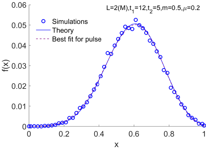
Now that we have $q_{\textbf{A}}(\ell)$ and $q_{\textbf{B}}(\ell)$ for the two-wave model (Eqs. (10) and (6), respectively), we can use Eq. (4) for the distribution of the ancestry proportions. We inverted $\hat{f}(u;s)$ with respect to $u$ using Mathematica and then numerically with respect to $s$, to obtain $f(x;L)$. Simulation results are shown in Figure 3, demonstrating that our theoretical results fit the empirical data very well. Here too, excellent fit is achieved also by the pulse admixture model.

We proposed a simple method for inference of admixture parameters based on the empirical distribution of the proportion of each chromosome that descend from each source population. One advantage of this approach is not having to rely on the precise boundaries of the admixture segments. Rather, we only need the total amount of genetic material from each source, which is typically easier to estimate, even without explicitly performing local ancestry inference (e.g., using programs such as ADMIXTURE). Additionally, our method is easily adapted to unphased data, and enjoys the advantages of maximum likelihood estimation. Finally, we were able to completely generalize the results to the case of two-wave admixture, where gene flow from one of the populations occurred in two different occasions.

Extending the results to additional gene flow events (limited to a single source population) should be straightforward, at least numerically. However, extensions to more complex models or to continuous migration seem complicated. The finite population size could generally be neglected, as long as it is much larger than the sample size and (numerically) than the number of generations since admixture, which is typically the case. For small populations, genetic drift has two contrasting effects. The first is to increase the variance of the distribution of the ancestry proportions, since the potential for a “back-coalescence” implies that recombination events do not always change the ancestry, effectively increasing segment lengths. Based on the analysis of the SMC’ model by Liang and Nielsen (2014a), Eq. (1) should still hold, but with $h=tL$ replaced by $h=\tau L$, where $\tau=2N\left(1-e^{-t/(2N)}\right)$ (derivation not shown; note that $\tau\rightarrow t$ for $t\ll 2N$). The second effect arises when the distribution is over a sample from the population, reducing the variance due to the fact that lineages may coalesce already before reaching the time of admixture. A complete theory is yet to be developed, perhaps along the lines of Liang and Nielsen (2014b).

While our results provide reasonable accuracy for a parameter regime typical of some natural populations, we caution that often, the method may not be directly applicable. Intuitively, the information exploited by our method is mostly in the first moments of the distribution; while we estimate parameters in a more principled MLE approach, our method is still prone to inaccuracies in estimating ancestry proportions, as in studies based merely on the variance (e.g., (Botigué et al., 2013) and our unpublished results for Ashkenazi Jews). Nevertheless, our method may serve as a building block (or a sanity check) for more complex approaches. For example, our results already clearly demonstrate the inherent infeasibility of distinguishing a pulse and a two-wave admixture histories using segment lengths and ancestry proportions statistics for recent admixture (past $\approx 10$ generations). Finally, our theoretical results will be of great interest to researchers in population genetics and coalescent theory working in the very active field of admixture modeling.

Matlab code is available for the inference of $m$ and $t$ for the pulse admixture model, as well as for the distributions of segment lengths and ancestry proportions for the two-wave model. See https://github.com/scarmi/admixture_models.

S.C. thanks the Human Frontier Science Program for financial support.

References

- Alexander et al. (2009) Alexander, D. H., Novembre, J., Lange, K., 2009. Fast model-based estimation of ancestry in unrelated individuals. Genome Res. 19, 1655–1664.
- Botigué et al. (2013) Botigué, L. R., Henn, B. M., Gravel, S., Maples, B. K., Gignoux, C. R., Corona, E., Atzmon, G., Burns, E., Ostrer, H., Flores, C., Bertranpetit, J., Comas, D., Bustamante, C. D., 2013. Gene flow from North Africa contributes to differential human genetic diversity in Southern Europe. Proc. Natl. Acad. Sci. USA 110, 11791–11796.
- Brisbin et al. (2012) Brisbin, A., Bryc, K., Byrnes, J., Zakharia, F., Omberg, L., Degenhardt, J., Reynolds, A., Ostrer, H., Mezey, J. G., Bustamante, C. D., 2012. Pcadmix: principal components-based assignment of ancestry along each chromosome in individuals with admixed ancestry from two or more populations. Hum. Biol. 84, 343–364.
- Excoffier et al. (2013) Excoffier, L., Dupanloup, I., Huerta-Sanchez, E., Sousa, V. C., Foll, M., 2013. Robust demographic inference from genomic and snp data. PLoS Genet. 9, e1003905.
- Godrèche and Luck (2001) Godrèche, C., Luck, J. M., 2001. Statistics of the occupation time of renewal processes. J. Stat. Phys. 104, 489.
- Goldberg and Rosenberg (2015) Goldberg, A., Rosenberg, N. A., 2015. Beyond 2/3 and 1/3: the complex signatures of sex-biased admixture on the X chromosome. Genetics 201, 263–279.
- Goldberg et al. (2014) Goldberg, A., Verdu, P., Rosenberg, N. A., 2014. Autosomal admixture levels are informative about sex bias in admixed populations. Genetics 198, 1209–1229.
- Gravel (2012) Gravel, S., 2012. Population genetics models of local ancestry. Genetics 191, 607–619.
- Gutenkunst et al. (2009) Gutenkunst, R. N., Hernandez, R. D., Williamson, S. H., Bustamante, C. D., 2009. Inferring the joint demographic history of multiple populations from multidimensional snp frequency data. PLoS Genet. 5, e1000695.
- Hellenthal et al. (2014) Hellenthal, G., Busby, G. B., Band, G., Wilson, J. F., Capelli, C., Falush, D., Myers, S., 2014. A genetic atlas of human admixture history. Science 343, 747–751.
- Johnson et al. (2011) Johnson, N. A., Coram, M. A., Shriver, M. D., Romieu, I., Barsh, G. S., London, S. J., Tang, H., 2011. Ancestral components of admixed genomes in a mexican cohort. PLoS Genet. 7, e1002410.
- Liang and Nielsen (2014a) Liang, M., Nielsen, R., 2014a. The lengths of admixture tracts. Genetics 197, 953–967.
- Liang and Nielsen (2014b) Liang, M., Nielsen, R., 2014b. Understanding admixture fractions. bioRxiv.
- Loh et al. (2013) Loh, P. R., Lipson, M., Patterson, N., Moorjani, P., Pickrell, J. K., Reich, D., Berger, B., 2013. Inferring admixture histories of human populations using linkage disequilibrium. Genetics 193, 1233–1254.
- Maples et al. (2013) Maples, B. K., Gravel, S., Kenny, E. E., Bustamante, C. D., 2013. Rfmix: a discriminative modeling approach for rapid and robust local-ancestry inference. Am. J. Hum. Genet. 93, 278–288.
- Margolin and Barkai (2004) Margolin, G., Barkai, E., 2004. Aging correlation functions for blinking nanocrystals, and other on-off stochastic processes. J. Chem. Phys. 121, 1566–1577.
- Moorjani et al. (2011) Moorjani, P., Patterson, N., Hirschhorn, J. N., Keinan, A., Hao, L., Atzmon, G., Burns, E., Ostrer, H., Price, A. L., Reich, D., 2011. The history of african gene flow into southern europeans, levantines, and jews. PLoS Genet. 7, e1001373.
- Moreno-Mayar et al. (2014) Moreno-Mayar, J. V., Rasmussen, S., Seguin-Orlando, A., Rasmussen, M., Liang, M., Flam, S. T., Lie, B. A., Gilfillan, G. D., Nielsen, R., Thorsby, E., Willerslev, E., Malaspinas, A. S., 2014. Genome-wide ancestry patterns in Rapanui suggest pre-European admixture with Native Americans. Curr. Biol. 24, 2518–2525.
- Ni et al. (2015) Ni, X., Yang, X., Guo, W., Yuan, K., Zhou, Y., Ma, Z., Xu, S., 2015. Length distribution of ancestral tracks under a general admixture model and its applications in population history inference. bioRxiv.
- Palamara and Pe’er (2013) Palamara, P. F., Pe’er, I., 2013. Inference of historical migration rates via haplotype sharing. Bioinformatics 29, i180–188.
- Patterson et al. (2012) Patterson, N., Moorjani, P., Luo, Y., Mallick, S., Rohland, N., Zhan, Y., Genschoreck, T., Webster, T., Reich, D., 2012. Ancient admixture in human history. Genetics 192, 1065–1093.
- Pickrell et al. (2014) Pickrell, J. K., Patterson, N., Loh, P.-R., Lipson, M., Berger, B., Stoneking, M., Pakendorf, B., Reich, D., 2014. Ancient west Eurasian ancestry in southern and eastern Africa. Proc. Natl. Acad. Sci. USA 111, 2632–2637.
- Pool and Nielsen (2009) Pool, J. E., Nielsen, R., 2009. Inference of historical changes in migration rate from the lengths of migrant tracts. Genetics 181, 711–719.
- Price et al. (2009) Price, A. L., Tandon, A., Patterson, N., Barnes, K. C., Rafaels, N., Ruczinski, I., Beaty, T. H., Mathias, R., Reich, D., Myers, S., 2009. Sensitive detection of chromosomal segments of distinct ancestry in admixed populations. PLoS Genet. 5, e1000519.
- Pritchard et al. (2000) Pritchard, J. K., Stephens, M., Donnelly, P., 2000. Inference of population structure using multilocus genotype data. Genetics 155, 945–959.
- Pugach et al. (2011) Pugach, I., Matveyev, R., Wollstein, A., Kayser, M., Stoneking, M., 2011. Dating the age of admixture via wavelet transform analysis of genome-wide data. Genome Biol. 12, R19.
- Sanderson et al. (2015) Sanderson, J., Sudoyo, H., Karafet, T. M., Hammer, M. F., Cox, M. P., 2015. Reconstructing past admixture processes from local genomic ancestry using wavelet transformation. Genetics 200, 469–481.
- Stam (1980) Stam, P., 1980. The distribution of the fraction of the genome identical by descent in finite random mating populations. Genet. Res. 35, 131–155.
- Verdu and Rosenberg (2011) Verdu, P., Rosenberg, N. A., 2011. A general mechanistic model for admixture histories of hybrid populations. Genetics 189, 1413–1426.