Quantifying noise sources in the KSTAR 2014 Thomson Scattering system from the measured variation on electron temperature

Thomson scattering (TS) systems are widely used to measure the temperature ($T_{e}$) and density ($n_{e}$) of electrons in fusion devices. KSTAR Thomson scattering system consists of separate core and edge collection optics collecting the Thomson scattered photons which are transmitted to polychromators via optical fibres [1, 2]. After the band-pass filters, where Figure 1 shows an example of the measured filter functions, optical signals are converted to electrical signals and recorded with the newly installed fast sampling digitizers (NI PXIe-5160) with the sampling rate of either $1.25$ or $2.5$ GS/s, in addition to the existing charge-integrating (gating) digitizer.

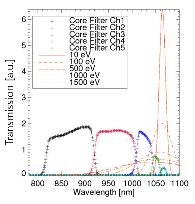
We use a weighted look-up table method to estimate the time evolution of electron temperature while exclusively considering the uncertainty due to the background noise. Another possibly large source of uncertainty may originate from the photon (Poisson) noise. However, the photon noise could not be reflected in our analysis due to the lack of absolute photon counts. Note that the absolute photon counts can be estimated based on Rayleigh or rotational Raman calibration [3, 4], but such data have not been obtained with the fast sampling digitizers during the 2014 KSTAR campaign. Rayleigh calibration data are obtained only with the existing charge-integrating (gating) digitizers.

Estimated electron temperature shows scatters, i.e., $15$% variation on $T_{e}$ with respect to its mean value. By using the synthetic data, we have found that this scattering on $T_{e}$ cannot be explained solely by the uncertainty due to the background noise. Our main goal of this paper is to estimate the ‘total’ noise level of the Thomson signal consistent with the observed variation on $T_{e}$ using the synthetic data. With the levels of estimated total noise and the measured background noise, we deduce the photon noise level assuming that photon noise and background noise are uncorrelated. We confirm that photon noise prevails over the background one for the Thomson data from the 2014 KSTAR campaign.

A polychromator contains five channels consisting of five band-pass filters shown in Figure 1 with five photon detectors (IR-enhanced Si APD: Hamamatsu S11519).

Figure 2 shows an example of the Thomson signal from each channel. Although the background noise levels are quite similar for all five channels, ch 1 does not show observable Thomson scattered signal. This may be due to electron temperature being less than $1$ keV (see Figure 1). The signal from ch 5 is mostly due to the straylight as attested by the fact that the signal levels before and during plasma shots are identical (not shown in the figure). The level of Thomson signal from ch 4 is smaller compared to signals obtained from chs 2 and 3, again perhaps due to not-high enough electron temperature.

To estimate the integral of the $i$th channel Thomson signal $A_{TS}^{i}$, we perform a Gaussian fitting to the Thomson signal $V_{TS}^{i}$ (red line in Figure 2) which can be written as [4]

where $G$ is the APD gain factor, $n_{laser}\left(t\right)$ the number of photons per unit time as a function of time where $\int dt\>n_{laser}\left(t\right)=N_{laser}$ is the total number of photons in a single laser pulse. $\frac{\mathrm{d}\sigma_{TS}}{\mathrm{d}\Omega}$ is the differential Thomson scattering cross-section area, $\Delta Q$ the solid angle of the TS system and $L$ the scattering length. The net transmission coefficient of the collective optics $T(\lambda)$ is a function of the wavelength, but we assume that it is constant within the range of interests; hence $T(\lambda)=T(\lambda_{L})$ where $\lambda_{L}$ is the laser wavelength. As the $i$th channel filter function $\phi^{i}(\lambda)$ includes the wavelength variation of the quantum efficiency $QE$ of the APD detector, the value of $QE$ is taken at the laser wavelength. $S(\lambda,T_{e},\theta)$ is the spectral distribution of the scattered photons [5] where $\theta$ is the scattering angle. Then, $A_{TS}^{i}$ is simply

From Eq. (1), we find that the terms outside the integral do not depend on the channels. Thus, by taking the ratio of measured signals between the two channels such as

we can construct an equation that depends on only $T_{e}$ and $\theta$. Note that we have $\theta\approx 90^{\circ}$ in this study [6]. Defining $M^{i}\left(T_{e}\right)=\int d\lambda\>\phi^{i}(\lambda)\>S(\lambda,T_{e},\theta=90^{\circ})$, Figure 3 shows $M^{i}$ as a function of $T_{e}$ for all five channels. As we decide not to use signals from chs 1 and 5 due to indiscernible Thomson signals from the background noise or stray light, we create $\mathcal{R}^{ij}$ with chs 2, 3 and 4 which are shown in Figure 3.

Because we may find three different $T_{e}$’s based on the measurements from Figure 3, the $T_{e}$’s can be averaged with a weighting factor of the inverse of corresponding total uncertainty as

where $T_{e}^{ij}$ and $\sigma_{total}^{ij}$ are the estimated electron temperature using $\mathcal{R}^{ij}$ and its total uncertainty, respectively. $\sigma_{total}^{ij}$ can be estimated using a propagation of uncertainty assuming that the total uncertainty of the $i$th and $j$th channels, $\sigma_{total}^{i}$ and $\sigma_{total}^{j}$, are uncorrelated. Ideally, $\sigma_{total}^{i}$ needs to include both the background noise $\sigma_{bg}^{i}$ and the photon noise $\sigma_{ph}^{i}$:

However, not knowing the photon noise level, we estimate the $T_{e}$ by setting ${\sigma_{total}^{i}}=\sigma_{bg}^{i}$. In this paper, we estimate the background noise of the $i$th channel as

where $\delta^{i}$ is the standard deviation of the data in the blue shaded region shown in Figure 2. As shown in Figure 2, we first fit a Gaussian function to the Thomson signal which finds the amplitude, peak-time and width ($w$) of the Gaussian. The blue shaded region where we obtain the background noise level starts at $5w$ away from the peak-time assuming that no Thomson signal exists in this region, hence only the background signal. $N_{TS}^{i}$ is the number of data points within the fitted Gaussian, i.e., $N_{TS}^{i}=4w/\Delta t$, where $\Delta t$ is $0.8$ ns, the time step of the data points with $1.25$ GS/s. Figure 4 shows examples of the temporal evolution of $T_{e}$ for two different KSTAR plasma shots estimated using Eq. (4).

As the estimated $T_{e}$ shows about $15$% variation on $T_{e}$ with respect to its mean value (e.g. see Figure 4), we raise the following questions: 1) can the background noise explain such an observed variation on $T_{e}$? 2) if not, how large does $\sigma_{ph}^{i}$ have to be to explain the observation? To be able to answer these questions, we generate synthetic Thomson signal where we can vary the noise levels numerically.

By letting $n_{laser}\left(t\right)$ in Eq. (1) have a Gaussian form in a time domain (consistent with fitting the Gaussian function to measured Thomson signals), we generate the synthetic Thomson data for each channel similar to the measured data shown in Figure 2. We set the time step of synthetic data to be $0.8$ ns corresponding to $1.25$ GS/s of the fast sampling digitizer. A random number selected from a normal distribution is, then, added to each time point as a noise. The width of this normal distribution $\delta_{SYN}$ is set such that $\sigma_{SYN}=\delta_{SYN}\sqrt{N_{TS}^{i}}\Delta t$ (cf. Eq. (6)) controlling the noise level. This completes generating synthetic Thomson signal for a single laser pulse. Let us denote the $i$th channel synthetic Thomson signal as $V_{SYN}^{i}\left(t\right)$ and its integral as $A_{SYN}^{i}$ estimated by fitting a Gaussian function to the $V_{SYN}^{i}\left(t\right)$ as if it were real measured signal.

We define the signal-to-noise ratio (SNR) of $T_{e}$, $SNR_{T_{e}}$, and that of the measured (synthetic) Thomson signal from the $i$th channel, $SNR_{*}^{i}$ ($SNR_{SYN}^{i}$), to be

where the subscript $*$ takes any one of the total (‘total’), background (‘bg’) or photon (‘ph’) for the noise source, i.e., $SNR_{bg}^{i}$ indicates the SNR of the Thomson signal due to the background noise. Here, $\left<\cdot\right>$ indicates the time average with $50$ consecutive data points equivalent to the time duration of $0.5$ seconds, a couple of equilibrium evolution time scale for a typical KSTAR plasma, with the laser pulse repetition rate of $100$ Hz during the 2014 KSTAR campaign. $\sigma_{T_{e}}$ is the standard deviation of $T_{e}$ during the $0.5$ seconds. Figure 5 shows time evolution of $SNR_{T_{e}}$ and $SNR_{bg}^{i}$ for $i=2$, $3$ and $4$ for the plasma shots shown in Figure 4.

We wish to find $SNR_{total}^{i}$ and the corresponding $\sigma_{total}^{i}$ for $i=2,3$ and $4$ consistent with the experimentally measured $SNR_{T_{e}}$. Once we have $\sigma_{total}^{i}$, $\sigma_{ph}^{i}$ can be calculated using Eq. (5) with the measured $\sigma_{bg}^{i}$. Thus, we obtain $SNR_{total}^{i}$ and $\sigma_{total}^{i}$ with the synthetic data by recognizing that $SNR_{total}^{i}=SNR_{SYN}^{i}$ and $\sigma_{total}^{i}=\sigma_{SYN}^{i}$. Here, we face a problem: there may exist infinite number of solutions on the combination of $SNR_{total}^{i}$ for $i=2,3$ and $4$ consistent with the measured $SNR_{T_{e}}$. To circumvent such a problem, anticipated by the experimental observation, we generate synthetic data only for chs 2 and 3 and let $SNR_{SYN}^{i=2}=SNR_{SYN}^{i=3}$ since $SNR_{bg}^{4}<SNR_{bg}^{2}\sim SNR_{bg}^{3}$ (see Figure 5). We generate a database of $SNR_{T_{e}}=f\left(SNR_{SYN}^{i},T_{e}\right)$ for many different values of $\left<T_{e}\right>$ for $i=2$ and $3$. Figure 6 shows the level of $SNR_{T_{e}}$ estimated with the synthetic data as a function of $SNR_{SYN}^{i}$ at $\left<T_{e}\right>=800$ eV.

As the $SNR_{T_{e}}$ from the synthetic data has been estimated with only chs 2 and 3 (e.g. Figure 6), we recalculate the experimental $SNR_{T_{e}}$ using only these two channels as shown in Figure 7. Here, we also plot the ‘required’ level of $SNR_{total}^{i}$ (green square) using the database of $SNR_{T_{e}}=f\left(SNR_{SYN}^{i},T_{e}\right)$ which allows us to estimate $\sigma_{total}^{i}$ for $i=2$ and $3$ using Eq. (7).

Figure 8 shows, for the KSTAR #10433, the levels of total required noise obtained by the synthetic data, background noise from experimental data and photon noise with Eq. (5) normalized to the experimental signal levels for chs 2 and 3. It is clear that the KSTAR Thomson scattering system during 2014 campaign is photon noise dominated at least for the chs 2 and 3 of the polychromator we have investigated. This is good that the system is not limited by the background noise, however it also suggests that the system needs to collect more photons and utilize the collected photons more efficiently to reduce the $15$% variation on the measured $T_{e}$.

From the estimated normalized photon noise level, i.e., $1/SNR_{ph}^{i}$, we can estimate the ‘effective’ photon counts $N_{ph}^{i,~eff}$ detected by the photon detectors as

where $F$ is the noise factor defined as the ratio of the input SNR to the output SNR [4], and $N_{ph}^{i}$ is the ‘actual’ photon counts. Using the values from Figure 8 and Eq. (8), we find that the effective photon counts are approximately $170$ for chs 2 and 3. Note that the noise factor $F$ is always greater than or equal to $1$, thus actual photon counts may well be larger than $170$, i.e., by a factor of $F^{2}$. However, this cannot be regarded as the gain in photon counts since $F$ decreases the SNR.

The core KSTAR 2014 TS system has an effective F/# of $6.7$ which corresponds to $17.5$ msr. With the incident laser wavelength of $1064$ nm and energy of $2.0$ J, the incident photon number is estimated to be $1.1\times 10^{19}$. Having approximate values of effective quantum efficiency of $15$%, scattering length of $10$ mm, optical transmittance of $40$%, filter transmittance of $70$%, we estimate photon budget to be approximately 6,200 photons per $1.0\times 10^{19}$ m^-3 of electron density. For $T_{e}=800$ eV, we find that the optical band-pass filters for chs 2 and 3 covers about $30$% of the full spectrum (see Figure 1). Thus, the expected photon counts on chs 2 and 3 are approximately $1,800$ about an order of magnitude higher than the estimated effective photon counts. This means that the KSTAR TS system has large potential to be improved.

In this paper, we estimated the time evolution of electron temperature by using the weighted look-up table method and found a $15$% variation on $T_{e}$. By using the synthetic Thomson data, we have found that such a variation on electron temperature cannot be explained solely by the background noise and thus estimated the required uncertainty level consistent with the experimental observation. Our study indicates that the chs 2 and 3 of the polychromator we have investigated are dominated by the photon noise with the average effective photon counts per laser pulse of $170$. This suggests that improving the photon collection system and decreasing the noise factor of the system is required to decrease the observed scatters in electron temperature.