When Chiral Photons Meet Chiral Fermions –
Photoinduced Anomalous Hall Effects in Weyl Semimetals

Introduction - Previously thought to be an asset exclusive to massless elementary particles such as photons, chirality has now become a defining emergent property of electrons in such crystalline materials like graphene [1] and the surface of topological insulators [2]. An exciting new addition to the growing list of “chiral electronic materials”is the Weyl semimetal [3, 4, 5, 6, 7]. In this three-dimensional analogue of graphene, the Weyl nodes act as magnetic monopoles in momentum space [8]. In sharp contrast to the two Dirac nodes in graphene that behave more or less as separate low-energy degrees of freedom, a pair of Weyl nodes carrying opposite chiralities are inherently tied together in a non-local manner through the “chiral anomaly” mechanism which allows the dissipationless transfer of charge between them [9]. The subject has undergone vigorous research lately due to reports of material predictions, followed immediately by their synthesis and confirmation of their Weyl characters by photoemission experiments and non-local transport measurements. A striking example of success along this line in recent years is the transition metal monophosphide family that includes TaAs, TaP, NbAs, and NbP [10, 11, 12, 13, 14, 15, 16, 17, 18, 19].

In light of the rapid maturity of the Weyl semimetal research, one should ask whether the unusual electronic transport properties in both the static and dynamic regimes of the Weyl semimetal can be exploited in high speed electronics or to provide a new means of revealing dynamic topological effects [18, 19, 20]. It was recently suggested that exposing a two-dimensional Dirac material to a circularly polarized (CP) light could lead to a novel form of Hall effect due to the effective gap opening at the Dirac point [21, 22]. A natural question arises as to what happens when the three-dimensional, linearly dispersing band of electrons couple to an intense CP light, as schematically presented in Fig. 1, and whether a non-trivial Hall effect can be induced. Here we present a direct consequence of coupling CP light to the Weyl fermion: the appearance of the anomalous Hall effect (AHE).

In this work, we show that even when the AHE is absent due to symmetry reasons in typical Weyl materials, it must be generally present in all Weyl systems when coupled to a CP light source. Based on a low-energy effective Weyl-Floquet Hamiltonian analysis and symmetry considerations, we discuss the induced AHE as a generic and readily observable phenomenon in Weyl semimetals. We further demonstrate this effect using a concrete microscopic model, and apply our study to the TaAs family of Weyl semimetals with an estimation of the experimental feasibility. Other interesting works have addressed the driven three-dimensional Dirac electrons [23, 24] or gapped systems [25, 26]. However, neither systems enjoy the unique topological protection of the Weyl nodes, whose response, under a CP beam, results in the experimental signature of the AHE as we explain below.

General tight-binding model analysis: The low-energy Hamiltonian for a single Weyl node can be parameterized most generally by a real 3-vector $\vec{\alpha}$ and a $3\times 3$ real matrix $\beta$:

with a canonical 3D linear dispersion $E_{W}(\vec{q})=\alpha_{i}q_{i}\pm[\sum_{j}(\sum_{i}q_{i}\beta_{ij})^{2}]^{1/2}$. Einstein summation is assumed in the momentum $q_{i}$ and the Pauli matrix $\sigma_{j}$. The chirality of the Weyl node is given by the sign of the determinant of $\beta$: $\chi_{W}=\mbox{sgn}[\mbox{Det}(\beta)]$. For a practical band structure, this 2$\times$2 Weyl Hamiltonian is embedded within a large $N$-band Hamiltonian as a low-energy sector. In order to have the most general consideration of the photoinduced AHE, we therefore consider a $N$-band tight-binding Hamiltonian $H(\vec{k})$. The expansion of $H(\vec{k})$ around a Weyl node at $\vec{k}_{W}$ to first order in $\vec{q}=\vec{k}-\vec{k}_{W}$ can be put in the block form:

where the matrix $D_{0}$ gives the $(N-2)$ high-energy states at $\vec{k}=\vec{k}_{W}$. Eigenvectors at $\vec{k}=\vec{k}_{W}$ are used to construct the unitary matrix $U$ whose first two columns corresponding to the two zero-energy states. In general, the $2\times(N-2)$ matrices $C_{i}$ mix the Weyl bands with high-energy bands linearly in $\vec{q}$ and should not be ignored.

Without loss of generality, we consider an incident electromagnetic wave in the $z$-direction with the vector potential $\vec{A}(t)=(A_{x}\cos(\omega t),A_{y}\sin(\omega t+\phi),0)$. Following standard routes [21], the Peierls substitution $H_{\rm lin}(\vec{q})\rightarrow H_{\rm lin}(\vec{q}+e\vec{A}(t))$ and averaging over one drive cycle leads to the effective Hamiltonian [27]:

where the $2\times 2$ Weyl-Floquet part reads

Higher-order terms $O(q^{2})+O(qA^{2})+O(A^{4})$ are ignored. Clearly, the photoinduced effect is maximized for a CP light when $\cos\phi=\pm 1$, and vanishes for a linearly polarized beam.

The CP light has two contributions to the Weyl-Floquet Hamiltonian in Eq. (4). The first ($\beta^{2}$) term originates entirely from the two-band Weyl Hamiltonian $H_{\rm W}(\vec{q})$, while the second term proportional to $C_{x}C_{y}^{\dagger}-C_{y}C_{x}^{\dagger}$ is due to high-energy band-mixing and must be kept in the construction of a general Weyl-Floquet effective model. For later convenience, we re-parameterize $-(i/2)(C_{x}C_{y}^{\dagger}-C_{y}C_{x}^{\dagger})=\kappa_{0}\sigma_{0}+\kappa_{i}\sigma_{i}$ with four real numbers $\kappa_{i}=(-i/4)\mbox{Tr}[\sigma_{i}(C_{x}C_{y}^{\dagger}-C_{y}C_{x}^{\dagger})]$. Therefore, the influence of the drive to $A^{2}$-order on the $2\times 2$ Weyl band can be summarized as:

$\delta q_{i}$ and $\delta\mu$ represent the shifts of Weyl momenta and chemical potential, respectively.

The photoinduced Weyl node shift has an immediate consequence on the electronic transport. According to Ref. [6], for a Weyl system where the chemical potential situates at the nodes (i.e. $\mu=0$), the leading order change of the anomalous Hall conductivity is governed by the momentum shifts of every Weyl node as:

Different Weyl nodes are labeled by the superscript $I$ and $\delta\vec{\nu}$ is the change of the Chern vector [6]. Provided that the momentum shifts $\delta q^{(I)}_{k}$ among Weyl nodes of different chiralities $\chi_{W}^{(I)}$ do not cancel out, one would expect the AHE induced at the $A^{2}$-order proportional to the intensity of the incident beam. Note that the photoinduced self-doping ($\delta\mu\neq 0$) of the Weyl nodes contributes to $\delta\sigma_{ij}$ at a higher order $O(\delta\mu^{2})=O(A^{4})$ [6] of the drive intensity, which is negligible. If $\vec{\kappa}^{(I)}=0$, one can show the $z$-component of the Chern vector shift to be

where $\mbox{Cof}(\beta^{(I)})_{ij}$ is the $ij$ element of the cofactor matrix of $\beta^{(I)}$. The alternating signs of $\chi^{(I)}$ between a node and an anti-node, or a monopole and an anti-monopole, are precisely cancelled by the same sign change in $\delta q^{(I)}_{z}$. As such, each Weyl node has a positive-definite contribution to $\delta\nu_{z}$. Consequently, a finite Hall conductivity is induced in the plane perpendicular to the incident beam and its sign is determined by the photon chirality through $\sigma_{xy}\propto\cos\phi$.

In practice, the pre-drive chemical potential $\mu$ may not cross the Weyl node as we discussed so far. As long as $\mu$ before the drive lies in the linearly dispersive regime near the node, one can show that the our resultant $\delta\sigma_{ij}$ is unaffected [27]. In fact, using a frequency of excitation $0<\omega<2\mu$ for slightly electron-doped Weyl node would ensure no absorption, as assumed here, and thus should lead to a more straightforward analysis of the experimental results regarding the photoinduced AHE.

Symmetry consideration for multiple Weyl nodes: In a typical Weyl material, there are multiple sets of Weyl nodes related by the space group and time-reversal (TR) symmetries [5, 10]. The parameters $\vec{\alpha}$, $\beta$, and $C_{i}$ characterizing symmetry-related nodes transform accordingly. We now derive their transformation rules and discuss how the nodal shifts $\delta\vec{q}$ and $\delta\mu$ among the symmetry-related nodes are correlated.

A pair of Weyl points $\vec{k}_{\rm W}^{(I)}$ (with $I=1,2$) related by some space-group symmetry satisfy $R\vec{k}_{W}^{(1)}=\vec{k}_{W}^{(2)}$, where $R\in O(3)$ defines the particular symmetry operation. The parameters quantifying the Weyl nodes transform according to

As a result, the chiralities of nodes related by a rotation ($\mbox{Det}[R]=+1$) are the same, whereas a mirror or inversion operation ($\mbox{Det}[R]=-1$) produces a sign difference. On the other hand, nodes related by an anti-unitary symmetry involving TR operation satisfy

Due to the presence of $\xi=(\xi_{lj})=\mbox{diag}(1,-1,1)$, the chiralities of these two nodes are related by $-\mbox{Det}[R]$. For instance, the TR operation with $R={\rm diag}(-1,-1,-1)$ gives the same chirality for the nodes at $\vec{k}_{\rm W}$ and $R\vec{k}_{\rm W}=-\vec{k}_{\rm W}$.

Some proposed Weyl semimetals break TR symmetry but preserve inversion (I). Our symmetry analysis predicts $\vec{\alpha}^{(2)}=-\vec{\alpha}^{(1)}$, $\beta^{(2)}=-\beta^{(1)}$, $\kappa_{0}^{(2)}=\kappa_{0}^{(1)}$ and $\vec{\kappa}^{(2)}=\vec{\kappa}^{(1)}$ for a pair of I-related nodes and thus, using Eq. (5),

Since these two nodes must have opposite chiralities ($\mbox{Det}[R]=-1$), the product $\chi^{(I)}\delta\vec{q}^{(I)}$ is identical for both of them. Hence, from Eq. (6), these two nodes contribute additively to the Hall conductivity. A similar conclusion holds for an I symmetry breaking Weyl materials for which TR is a good symmetry. In this case we find $\vec{\alpha}^{(2)}=-\vec{\alpha}^{(1)}$, $\beta^{(2)}=-\beta^{(1)}\cdot\xi$, $\kappa_{0}^{(2)}=-\kappa_{0}^{(1)}$ and $\vec{\kappa}^{(2)}=-\xi\cdot\vec{\kappa}^{(1)}$ for TR-related nodes, and thus

Since $\chi^{(1)}=\chi^{(2)}$, Eq. (6) once again predicts a constructive contributions from the TR-related nodes.

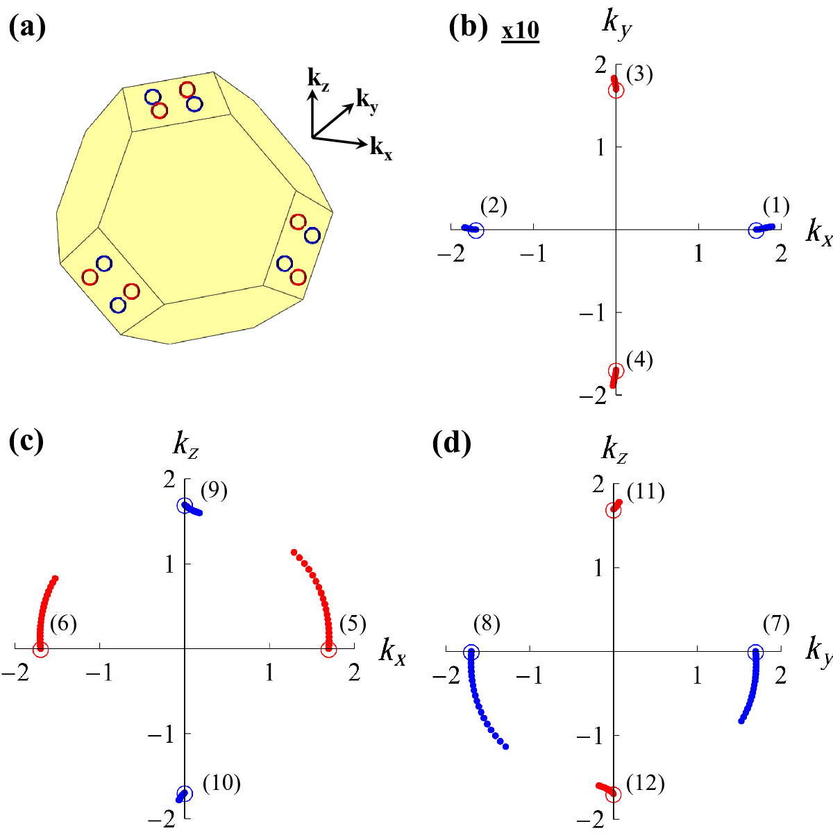
Lattice model analysis: To illustrate our findings, we now proceed to study a concrete lattice model for Weyl semimetal of inversion symmetry breaking type [28]. The model is parameterized by the hopping (t), spin-orbit coupling ($\lambda$) and inversion breaking potential ($\epsilon$) [27]. The bare system possesses $12$ Weyl nodes labeled as (see Fig. 2(a)):

along with their chiralities as subscripts $\pm$ and a characteristic momentum $k_{0}=2\sin^{-1}[\epsilon/(4\lambda)]$. In the presence of a CP drive, each node undergoes a momentum shift given by:

with $\eta=\sqrt{1-\epsilon^{2}/16\lambda^{2}}$. The momentum shifts clearly correlate with the chiralities. The photoinduced self-dopings are:

and $\delta\mu^{(1-8)}=0$. The anomalous Hall conductivity obtained is (up to $A^{2}$-order):

which agrees with the expectation of the low-energy analysis.

So far all our discussion have been done within the effective Hamiltonian scheme valid for a small driving amplitude. A more stringent check free from this assumption is offered by solving the full Floquet Hamiltonian whose matrix elements are $\langle n^{\prime}|H_{F}|n\rangle=H_{n-n^{\prime}}+n\omega\delta_{n,n^{\prime}}I_{4}$ with $n(n^{\prime})$ denoting the $n(n^{\prime})$-th Floquet band. The topological character of the Weyl nodes indeed protects them against the drive, and only their locations are shifted continuously in a chirality-dependent way. Figure 2(b-d) demonstrate the Weyl node shifts obtained from diagonalizing the full Floquet Hamiltonian as we increase the driving field strength. It is obvious that nodes with opposite chirality have opposite shifts in $k_{z}$, leading to an imbalance of $\delta\nu_{z}$ and eventually, a net anomalous Hall conductivity. The overall field dependence of the sum of $\Delta k_{z}$ weighted by chiralities is shown in Fig. 3(a), which exhibits the anticipated $A^{2}$ increment (we have put $e=1$). This quantity equals to the Chern vector $\delta\nu_{z}$ in the small $A$ regime (Eq. (6)). On the other hand, the resultant self-doping shows the expected $A^{2}$ dependence as illustrated in Figure 3(b). However, it only corresponds to a higher order effect and does not affect the photoinduced AHE.

Application to TaAs family of Weyl semimetals: TaAs was recently shown to host 24 Weyl nodes in the Brillouin zone [10, 15, 11]. There are two nonequivalent sets of Weyl points [10] that we denote as: the P-set consisting of $8$ nodes at $(\pm k^{P}_{x},\pm k^{P}_{y},0)$ and $(\pm k^{P}_{y},\pm k^{P}_{x},0)$, and the Q-set with $16$ nodes at $(\pm k^{Q}_{x},\pm k^{Q}_{y},\pm k_{z}^{Q})$ and $(\pm k^{Q}_{y},\pm k^{Q}_{x},\pm k_{z}^{Q})$. The values of $k^{P}_{x},k^{P}_{y},k^{Q}_{x},k^{Q}_{y},k_{z}^{Q}$ for various TaAs family of materials can be found in Ref. [10]. Applying the symmetry transformation rules derived before, we find a simple rule for the node shifts for both Weyl sets:

where $\delta q_{z}^{P(Q)}\propto A^{2}$ is the same for all $8(16)$ symmetry-related nodes. The $z$-direction momentum shift faithfully follows the chirality $\chi^{(I)}$ of each Weyl node, whereas the same is not true for the shifts in the xy-plane. Therefore, the overall photoinduced AHE for TaAs family is:

Experimental Realization: To guide future experimental efforts to observe these effects, we discuss the conditions needed and likelihood of success. In the supplemental we detail our calculations of the magnitude of the Hall voltage [27], where we assume the use of a CW CO₂ laser, with a roughly constant illumination across the contacts, spaced $\approx 100~\mu$m apart. Using established values for the Fermi velocity [16, 13, 20], reflectance, optical [29] and DC conductivities [18], we find a $100~\rm nm$ thick film [30] of TaAs would produce a Hall signal $\approx 130~nV$ at room temperature, with a DC current of 1A and 1W laser power. We note that the small penetration depth requires the use of thinner samples to ensure most of the current is modulated by the light (the induced voltage is inversely proportional to the square of the thickness). While such signals should be straight forward to detect, even higher values may be possible through the use of pulsed lasers with higher peak electric fields, with the Hall signal detected through Faraday rotation measurements.

Conclusion: An assortment of analysis based on Floquet theory is carried out on models of Weyl semimetals to argue that the AHE is induced generically by applying an AC electromagnetic field of a definite chirality, in the plane orthogonal to the incident beam. This photoinduced AHE originates from the remarkable monopole nature of Weyl nodes. The induced Hall conductivity scales linearly and continuously with the field intensity. The nodal shift itself may be observable by the pump-probe ARPES, while the photoinduced AHE can be detected via DC transport or Faraday rotation experiment on films. Conceivably, the AC-field-driven AHE may exist in other materials possessing non-trivial band topology such as ferromagnetic metals [31].

Acknowledgements - PAL acknowledges support from DOE Grant No. DE-FG02-03- ER46076. KSB acknowledges support from the National Science Foundation under Grant No. DMR-1410846. JHH is supported by the NRF grant (No. 2013R1A2A1A01006430). YR is supported by the Alfred P. Sloan fellowship and National Science Foundation under Grant No. DMR-1151440.

References

- [1] A. H. Castro Neto, F. Guinea, N. M. R. Peres, K. S. Novoselov, and A. K. Geim, Rev. Mod. Phys. 81, 109 (2009).
- [2] M. Z. Hasan and C. L. Kane, Rev. Mod. Phys. 82, 3045 (2010).
- [3] C. Herring, Phys. Rev. 52, 365 (1937).
- [4] S. Murakami, New Journal of Physics 9, 356 (2007).
- [5] X. Wan, A. M. Turner, A. Vishwanath, and S. Y. Savrasov, Phys. Rev. B 83, 205101 (2011).
- [6] K.-Y. Yang, Y.-M. Lu, and Y. Ran, Phys. Rev. B 84, 075129 (2011).
- [7] A. A. Burkov and L. Balents, Phys. Rev. Lett. 107, 127205 (2011).
- [8] Z. Fang, N. Nagaosa, K. S. Takahashi, A. Asamitsu, R. Mathieu, T. Ogasawara, H. Yamada, M. Kawasaki, Y. Tokura, and K. Terakura, Science 302, 92 (2003).
- [9] H. Nielsen and M. Ninomiya, Physics Letters B 130, 389 (1983).
- [10] H. Weng, C. Fang, Z. Fang, B. A. Bernevig, and X. Dai, Phys. Rev. X 5, 011029 (2015).
- [11] S.-M. Huang, S.-Y. Xu, I. Belopolski, C.-C. Lee, G. Chang, B. Wang, N. Alidoust, G. Bian, M. Neupane, C. Zhang, S. Jia, A. Bansil, H. Lin, and M. Z. Hasan, Nat Commun 6, 7373 (2015a).
- [12] S.-Y. Xu, I. Belopolski, N. Alidoust, M. Neupane, G. Bian, C. Zhang, R. Sankar, G. Chang, Z. Yuan, C.-C. Lee, S.-M. Huang, H. Zheng, J. Ma, D. S. Sanchez, B. Wang, A. Bansil, F. Chou, P. P. Shibayev, H. Lin, S. Jia, and M. Z. Hasan, Science 349, 613 (2015a).
- [13] B. Q. Lv, H. M. Weng, B. B. Fu, X. P. Wang, H. Miao, J. Ma, P. Richard, X. C. Huang, L. X. Zhao, G. F. Chen, Z. Fang, X. Dai, T. Qian, and H. Ding, Phys. Rev. X 5, 031013 (2015a).
- [14] C.-C. Lee, S.-Y. Xu, S.-M. Huang, D. S. Sanchez, I. Belopolski, G. Chang, G. Bian, N. Alidoust, H. Zheng, M. Neupane, B. Wang, A. Bansil, M. Z. Hasan, and H. Lin, arXiv:1508.05999 (2015).
- [15] B. Q. Lv, N. Xu, H. M. Weng, J. Z. Ma, P. Richard, X. C. Huang, L. X. Zhao, G. F. Chen, C. E. Matt, F. Bisti, V. N. Strocov, J. Mesot, Z. Fang, X. Dai, T. Qian, M. Shi, and H. Ding, Nature Physics 11, 724 (2015b).
- [16] L. X. Yang, Z. K. Liu, Y. Sun, H. Peng, H. F. Yang, T. Zhang, B. Zhou, Y. Zhang, Y. F. Guo, M. Rahn, D. Prabhakaran, Z. Hussain, S.-K. Mo, C. Felser, B. Yan, and Y. L. Chen, Nature Physics 11, 728 (2015).
- [17] S.-Y. Xu, N. Alidoust, I. Belopolski, Z. Yuan, G. Bian, T.-R. Chang, H. Zheng, V. N. Strocov, D. S. Sanchez, G. Chang, C. Zhang, D. Mou, Y. Wu, L. Huang, C.-C. Lee, S.-M. Huang, B. Wang, A. Bansil, H.-T. Jeng, T. Neupert, A. Kaminski, H. Lin, S. Jia, and M. Zahid Hasan, Nat Phys 11, 748 (2015b).
- [18] X. Huang, L. Zhao, Y. Long, P. Wang, D. Chen, Z. Yang, H. Liang, M. Xue, H. Weng, Z. Fang, X. Dai, and G. Chen, Physical Review X 5, 031023 (2015b).
- [19] C. Zhang, S.-Y. Xu, I. Belopolski, Z. Yuan, Z. Lin, B. Tong, N. Alidoust, C.-C. Lee, S.-M. Huang, H. Lin, M. Neupane, D. S. Sanchez, H. Zheng, G. Bian, J. Wang, C. Zhang, T. Neupert, M. Z. Hasan, and S. Jia, arXiv:1503.02630 , 2630 (2015).
- [20] C. Shekhar, A. K. Nayak, Y. Sun, M. Schmidt, M. Nicklas, I. Leermakers, U. Zeitler, Y. Skourski, J. Wosnitza, Z. Liu, Y. Chen, W. Schnelle, H. Borrmann, Y. Grin, C. Felser, and B. Yan, Nature Physics 11, 645 (2015).
- [21] T. Oka and H. Aoki, Phys. Rev. B 79, 081406 (2009).
- [22] Y. H. Wang, H. Steinberg, P. Jarillo-Herrero, and N. Gedik, Science 342, 453 (2013).
- [23] A. Narayan, Phys. Rev. B 91, 205445 (2015).
- [24] S. Ebihara, K. Fukushima, and T. Oka, arXiv:1509.03673 (2015).
- [25] N. H. Lindner, G. Refael, and V. Galitski, Nat Phys 7, 490 (2011).
- [26] R. Wang, B. Wang, R. Shen, L. Sheng, and D. Y. Xing, Europhysics Letters 105, 17004 (2014).
- [27] See Supplemental Material for more details about the effective Weyl-Floquet Hamiltonian, the lattice model calculation, realistic experimental estimations and the doping effect.
- [28] T. Ojanen, Phys. Rev. B 87, 245112 (2013).
- [29] B. Xu, Y. M. Dai, L. X. Zhao, K. Wang, R. Yang, W. Zhang, J. Y. Liu, H. Xiao, G. F. Chen, A. J. Taylor, D. A. Yarotski, R. P. Prasankumar, and X. G. Qiu, arXiv:1510.00470 (2015).
- [30] The proposed film has a thickness larger than the lattice spacing by two orders of magnitude so that the momentum along the width is still a good quantum number.
- [31] N. Nagaosa, J. Sinova, S. Onoda, A. H. MacDonald, and N. P. Ong, Rev. Mod. Phys. 82, 1539 (2010).
Supplemental Material:
- [1] T. Oka and H. Aoki, Phys. Rev. B 79, 081406 (2009)
- [2] T. Ojanen, Phys. Rev. B 87, 245112 (2013).
- [3] J. H. Shirley, Phys. Rev. 138, B979 (1965).
- [4] B. Xu, Y. M. Dai, L. X. Zhao, et al., arXiv:1510.00470.
- [5] X. Huang, L. Zhao, Y. Long, et al., Phys. Rev. X 5, 031023 (2015).
- [6] L. X. Yang, Z. K. Liu, Y. Sun, et al., Nature Physics 11, 728 (2015).
- [7] B. Q. Lv, H. M. Weng, B. B. Fu, et al., Phys. Rev. X 5, 031013 (2015).
- [8] C. Shekhar, A. K. Nayak, Y. Sun, et al., Nature Physics, 11, 645 (2015).
- [9] Y. H. Wang, H. Steinberg, P. Jarillo-Herrero, and N. Gedik, Science 342, 453 (2013).
- [10] K.-Y. Yang, Y.-M. Lu, and Y. Ran, Phys. Rev. B 84, 075129 (2011).
- [11] P. Delplace, J. Li, and D. Carpentier, EPL 97, 67004 (2012).