跳到论文正文
W Papers独立论文阅读器 arXiv:1509.05182 论文正文 计算阅读时间 · 0%
引用这篇论文根据当前论文元数据生成,正式投稿前建议核对。


License: arXiv.org perpetual non-exclusive license
arXiv:1509.05182v2 [math.AP] 30 Sep 2015

Ground State Patterns and Phase Transitions of Spin-1 Bose-Einstein Condensates via Γ\Gamma-Convergence Theory

I-Liang Chern Note: chern@math.ntu.edu.tw Affiliation: National Center for Theoretical Science, National Taiwan University, Taipei, 106, Taiwan Affiliation: Institute of Applied Mathematical Science, National Taiwan University, Taipei, 106, Taiwan    Chiu-Fen Chou Note: chouchiufen@gmail.com Affiliation: Department of Applied Mathematics, National Chiao Tung University, Hsinchu 300, Taiwan    Tien-Tsan Shieh Note: ttshieh@ncts.ntu.edu.tw Affiliation: National Center for Theoretical Science, National Taiwan University, Taipei, 106, Taiwan
Abstract

We develop an analytic theory for the ground state patterns and their phase transitions for spin-1 Bose-Einstein condensates on a bounded domain in the presence of a uniform magnetic field. Within the Thomas-Fermi approximation, these ground state patterns are composed of four basic states: magnetic state, nematic state, two-component state and three-component state, separated by interfaces. A complete phase diagram of the ground state patterns are found analytically with different quadratic Zeeman energy qq and total magnetization MM for both ferromagnetic and antiferromagnetic systems. Using the Γ\Gamma-convergence technique, it is found that the semi-classical limits of these ground states minimize an energy functional which consists of interior interface energy plus a boundary contact energy. As a consequence, the interface between two different basic states has constant mean curvature, and the contact angle between the interface and the boundary obeys Young’s relation.

1 Introduction

1.1 The Gross-Pitaevskii equation for spin-1 BECs

In the 1920s, Bose and Einstein [9, 21] predicted a new state of matter. At very low temperature, very dilute Boson gases such as alkai gases tend to occupy their lowest quantum state. The de Broglie wave of the bosons is coherent and their lowest quantum state becomes apparent, called Bose-Einstein condensation (BEC). It was only recently, in 1995, BEC was first realized in laboratories by two groups independently, Cornell and Wieman as well as Ketterle [2, 18]. Through the mean field approximation and Hartree’s ansatz, the mean-field state of an NN-particle boson gases can be described by a complex order parameter ψ⁡(x,t)\psi(x,t). Its dynamics is modelled by the Gross-Pitaevskii equation [17, 25, 51]:

i​ℏ​∂tψ=δ​ℰ​[ψ]δ​ψ∗,where ​ℰ​[ψ]=∫H⁡(ψ)​𝑑x,i\hbar{\partial}_{t}\psi=\frac{\delta\mathcal{E}[\psi]}{\delta\psi^{*}},\qquad\textrm{where }\mathcal{E}[\psi]=\int H(\psi)\,dx,

and the Hamiltonian of the system is written as

H⁡(ψ):=ℏ22​m​|∇ψ|2+V⁡(x)​|ψ|2+β2​|ψ|4.H(\psi):=\frac{\hbar^{2}}{2m}|{\nabla}\psi|^{2}+V(x)|\psi|^{2}+\frac{\beta}{2}|\psi|^{4}.

Here, ψ∗\psi^{*} denotes the complex conjugate of ψ\psi, and δ​ℰ/δ​ψ∗\delta\mathcal{E}/\delta\psi^{*} is the variation of ℰ\mathcal{E} with respect to ψ∗\psi^{*}. The function V⁡(x)V(x) is the trap potential satisfying V⁡(x)→∞V(x)\to\infty as |x|→∞|x|\to\infty. The parameter mm is the mass of the boson, and β\beta is the product of the particle number NN and interaction strength. This interaction is attractive when β<0\beta<0 and repulsive when β>0\beta>0. This mean field model was rigorously justified as a limit of the NN-particle quantum system by Lieb et al. [35, 36] for the ground state cases and by Erdös et al. for the dynamic cases [22].

When an optical trap is applied to confine BECs, all their hyperfine spin states are active. Such a BEC with an internal spin freedom is called a spinor BEC [28, 47, 34] and was realized in laboratories with 23Na atoms in 1998 [54, 53, 31, 8]. In the mean field theory, a physical state of a spin-ff BEC is described by (2​f+1)(2f+1)-components of complex order parameters Ψ=(ψf,ψf−1,…,ψ0​…,ψ−f)T\Psi=(\psi_{f},\psi_{f-1},\dots,\psi_{0}\dots,\psi_{-f})^{T} and its dynamics is governed by a multi-component Gross-Pitaeviskii equation [28, 47]. In this paper, we concern ourself with a quantum system of the spin-1 BEC, whose dynamics are described by a generalized Gross-Pitaevskii equation

i​ℏ​∂tΨ=δ​ℰ​[Ψ]δ​Ψ†,ℰ⁡[Ψ]=∫H⁡(Ψ)​𝑑x,i\hbar{\partial}_{t}\Psi=\frac{\delta\mathcal{E}[\Psi]}{\delta\Psi^{\dagger}},\qquad\mathcal{E}[\Psi]=\int H(\Psi)\,dx, (1.1)

where Ψ=(ψ1,ψ0,ψ−1)T\Psi=(\psi_{1},\psi_{0},\psi_{-1})^{T} and the Hamiltonian is given in the form

H⁡(Ψ)\displaystyle H(\Psi) :=Hk​i​n​(Ψ)+Hp​o​t​(Ψ)+Hn​(Ψ)+Hs​(Ψ)\displaystyle:=H_{kin}(\Psi)+H_{pot}(\Psi)+H_{n}(\Psi)+H_{s}(\Psi)
:=ℏ22​m​|∇Ψ|2+V⁡(x)​|Ψ|2+cn2​|Ψ|4+cs2​|Ψ†​𝐅​Ψ|2.\displaystyle:=\frac{\hbar^{2}}{2m}|{\nabla}\Psi|^{2}+V(x)|\Psi|^{2}+\frac{c_{n}}{2}|\Psi|^{4}+\frac{c_{s}}{2}|\Psi^{\dagger}\mathbf{F}\Psi|^{2}.

Here, Ψ†:=(ψ1∗,ψ0∗,ψ−1∗)\Psi^{\dagger}:=(\psi_{1}^{*},\psi_{0}^{*},\psi_{-1}^{*}) and 𝐅=(Fx,Fy,Fz)\mathbf{F}=(F_{x},F_{y},F_{z}) is the spin-1 Pauli operator:

Fx=12​(010101010),Fy=i2​(0−1010−1010),Fz=(10000000−1).F_{x}=\frac{1}{\sqrt{2}}\left(\begin{array}[]{ccc}0&1&0\\ 1&0&1\\ 0&1&0\end{array}\right),F_{y}=\frac{i}{\sqrt{2}}\left(\begin{array}[]{ccc}0&-1&0\\ 1&0&-1\\ 0&1&0\end{array}\right),F_{z}=\left(\begin{array}[]{ccc}1&0&0\\ 0&0&0\\ 0&0&-1\end{array}\right).

The term cn2​|Ψ|4\frac{c_{n}}{2}|\Psi|^{4} represents the spin-independent interaction between bosons, whereas cs2​|Ψ†​𝐅​Ψ|2\frac{c_{s}}{2}|\Psi^{\dagger}\mathbf{F}\Psi|^{2} stands for the spin-exchange interaction between bosons. The spin-independent interaction is attractive if cn<0c_{n}<0 and repulsive if cn>0c_{n}>0. This BEC system is called ferromagnetic if cs<0c_{s}<0 and antiferromagnetic if cs>0c_{s}>0. In experiments, an example of a ferromagnetic system is the alkali atom 87Rb with cn≈7.793c_{n}\approx 7.793, cs≈−0.0361c_{s}\approx-0.0361 [2], whereas for the alkali atom 23Na, cn≈15.587c_{n}\approx 15.587 and cs≈0.4871c_{s}\approx 0.4871 [18], and it is an antiferromagnetic system.

We are interested in the ground state patterns of spin-1 BECs in the presence of an external uniform magnetic field. The interaction of atoms with the applied magnetic field, say B​z^B\hat{z}, introduces an additional energy, called the Zeeman energy:

ℰZ​e​e​[Ψ]=∫HZ​e​e​(Ψ)​𝑑x,HZ​e​e​(Ψ):=∑j=−11Ej​(B)​|ψj|2,\mathcal{E}_{Zee}[\Psi]=\int H_{Zee}(\Psi)\,dx,\qquad H_{Zee}(\Psi):=\sum_{j=-1}^{1}E_{j}(B)|\psi_{j}|^{2},

where Ej​(B)E_{j}(B) is the Zeeman energy shift for each component under the magnetic field B​z^B\hat{z}. It is convenient for later discussion to write the Zeeman energy HZ​e​eH_{Zee} as

HZ​e​e=∑j=−11Ej​(B)​|ψ−1|2=q⁡(|ψ1|2+|ψ−1|2)+p⁡(|ψ1|2−|ψ−1|2)+E0​(|ψ1|2+|ψ0|2​|+ψ−1|2),H_{Zee}=\sum_{j=-1}^{1}E_{j}(B)|\psi_{-1}|^{2}=q(|\psi_{1}|^{2}+|\psi_{-1}|^{2})+p(|\psi_{1}|^{2}-|\psi_{-1}|^{2})+E_{0}(|\psi_{1}|^{2}+|\psi_{0}|^{2}|+\psi_{-1}|^{2}),

where

p=12​(E−1−E1),q=12​(E−1+E1−2​E0).p=\frac{1}{2}(E_{-1}-E_{1}),\ q=\frac{1}{2}(E_{-1}+E_{1}-2E_{0}).

The parameters pp and qq are called linear and quadratic Zeeman energy, respectively, in the physics literature.

Notice that the Gross-Pitaevskii equation for spin-1 BECs possess two invariants: the total mass

𝒩⁡[Ψ]:=∫|Ψ|2​𝑑x=∫|ψ1|2+|ψ0|2+|ψ−1|2​𝑑x,\mathcal{N}[\Psi]:=\int|\Psi|^{2}\,dx=\int|\psi_{1}|^{2}+|\psi_{0}|^{2}+|\psi_{-1}|^{2}\,dx, (1.2)

and the total magnetization

ℳ⁡[Ψ]:=∫|ψ1|2−|ψ−1|2​𝑑x,\mathcal{M}[\Psi]:=\int|\psi_{1}|^{2}-|\psi_{-1}|^{2}\,dx, (1.3)

which can be derived by direct calculation. The ground states of the system are those physical states of lowest energy, given fixed total mass and fixed total magnetization. This defines a variational problem for ground states in the presence of a uniform magnetic field:

minΨ{ℰ[Ψ]:𝒩[Ψ]=N,ℳ[Ψ]=M}.\min_{\Psi}\left\{\mathcal{E}[\Psi]:\,\mathcal{N}[\Psi]=N,\mathcal{M}[\Psi]=M\right\}. (1.4)

where the energy takes the form

ℰ⁡[Ψ]\displaystyle\mathcal{E}[\Psi] =∫(Hk​i​n+Hp​o​t+Hn+Hs+q⁡(|ψ1|2+|ψ−1|2))​𝑑x+E0​N+p​M\displaystyle=\int\left(H_{kin}+H_{pot}+H_{n}+H_{s}+{q(|\psi_{1}|^{2}+|\psi_{-1}|^{2})}\right)\,dx+E_{0}N+pM
=∫ℏ22​m​|∇Ψ|2+V⁡(x)​|Ψ|2+cn2​|Ψ|4+cs2​|Ψ†​𝐅​Ψ|2+q⁡(|ψ1|2+|ψ−1|2)​𝑑x+E0​N+p​M.\displaystyle=\int\frac{\hbar^{2}}{2m}|{\nabla}\Psi|^{2}+V(x)|\Psi|^{2}+\frac{c_{n}}{2}|\Psi|^{4}+\frac{c_{s}}{2}|\Psi^{\dagger}\mathbf{F}\Psi|^{2}+q(|\psi_{1}|^{2}+|\psi_{-1}|^{2})\,dx+E_{0}N+pM.

It is observed that the parameter pp plays no role in minimization for fixed total magnetization MM. Thus, our goal is to study the ground state patterns and their phase transitions in the parameter plane (q,M)(q,M).

1.2 A brief survey of ground state problems

There are several studies concerned with ground states of spin-1 BEC systems. The existence of ground states for spin-1 BECs in three dimensions with |cs|<cn|c_{s}|<c_{n} was given in  [39]. The non-existence result in three dimensions for cn<0c_{n}<0 was given in  [4]. Other existence/non-existence results in one dimension are given in  [11].

In the case of no applied magnetic field, it is proven that the ground state is the so-called single mode approximation (SMA) for a ferromagnetic system. That is, the ground state has the form (γ1,γ0,γ−1)​ψ(\gamma_{1},\gamma_{0},\gamma_{-1})\psi, where γi∈ℝ+\gamma_{i}\in\mathbb{R}^{+}, and ψ\psi is a scalar field. On the other hand, the ground state is a so-called two-component state (2​C)(2C) for antiferromagnetic systems. The above results are given numerically in  [37, 13], and analytically in  [38].

When there is an applied magnetic field, it is found that there is a phase transition from 2C to 3C, i.e. all three components are not zeros , as q>qc​r>0q>q_{cr}>0 for antiferromagnetic systems. This phase transition phenomenon was also observed in the laboratory [54, 32]. It was found numerically in  [59, 37, 14] and proven analytically in  [39].

Due to the fact that the coefficient ℏ22​m≪1\frac{\hbar^{2}}{2m}\ll 1, people have paid attention to the Thomas-Fermi approximation of (1.4) which simply ignores its kinetic energy. Under such an approximation, existence results for ground states and phase transitions with |cs|<<cn|c_{s}|<<c_{n} have also been studied by many physicists, see [59, 42, 40, 41].

Without ignoring the kinetic energy, the problem (1.4) is a variational problem of singular perturbation type which is similar to the Van der Waals-Cahn-Hilliard gradient theory of phase transition for a fluid system of binary phases confined to a bounded domain under isothermal conditions. Gurtin [27] had conjectured about the asymptotic behavior of the variational model

inf{∫Ω(ϵ|∇u|2+1ϵW(u)):u∈W1,2(Ω),∫Ωu(x)dx=m},\inf\left\{\int_{\Omega}\left(\epsilon|\nabla u|^{2}+\frac{1}{\epsilon}W(u)\right):\,u\in W^{1,2}(\Omega),\int_{\Omega}u(x)\,dx=m\right\},

where W:ℝn→ℝ+W:\mathbb{R}^{n}\to\mathbb{R}^{+} is a double-well potential and mm is the total mass of the fluid. The problem have been studied extensively by many authors through de Giorgi’s Γ\Gamma-convergence theory. The scalar case (n=1n=1) is studied by [43, 33, 55]. In [24, 55, 56], the vectorial case (n>1n>1) is studied. With a given Dirichlet boundary condition, a sharp interface limit of the energy functional is considered in [30, 49, 52]. A minimal interface problem arising from a two-component BEC in the regime of strong coupling and strong segregation was studied in [1] via Γ\Gamma-convergence. They have formulated the problem in term of total density and spin functions, which convert the energy into a sum of two weighted Cahn-Hilliard energy.

1.3 Contribution of this paper

This paper considers ground state patterns and their phase transition diagram on the qq-MM plane for the case |cs|<cn|c_{s}|<c_{n}. The contribution of this paper includes

  • •

    we find all possible ground states configurations for the spin-1 BEC system in its Thomas-Fermi approximation and give a complete phase diagram on the parameter space (q,M)(q,M);

  • •

    a sharp interface limit of the BEC system is derived through de Gorgi’s Γ\Gamma-convergence.

This paper is organized as the follows. Section 2 is a reformulation and simplification of the problem. Section 3 and 4 are devoted to the Thomas-Fermi approximations and the Γ\Gamma-convergence results.

2 Formulation of the problem

In this Section, the variational problem (1.4) for ground states of the spin-1 BEC system is formulated into a real-valued variational problem with dimensionless coefficients.

Dimensional Analysis

We minimize the energy function ℰ⁡[Ψ]\mathcal{E}[\Psi] under the two constraints (1.2), (1.3). The corresponding Euler-Lagrange equations read

(μ+λ)​ψ1\displaystyle(\mu+\lambda)\psi_{1} =\displaystyle= [−ℏ22​m​∇2+V⁡(x)+q+c0​n]​ψ1+c2​(n1+n0−n−1)​ψ1+c2​ψ−1∗​ψ02\displaystyle\left[-\frac{\hbar^{2}}{2m}{\nabla}^{2}+V(x)+q+c_{0}n\right]\psi_{1}+c_{2}(n_{1}+n_{0}-n_{-1})\psi_{1}+c_{2}\psi_{-1}^{*}{\psi_{0}}^{2}
μ​ψ0\displaystyle\mu\psi_{0} =\displaystyle= [−ℏ22​m​∇2+V⁡(x)+c0​n]​ψ0+2​c2​(n1−n−1)​ψ0+c2​ψ1​ψ−1​ψ0∗\displaystyle\left[-\frac{\hbar^{2}}{2m}{\nabla}^{2}+V(x)+c_{0}n\right]\psi_{0}+2c_{2}(n_{1}-n_{-1})\psi_{0}+c_{2}\psi_{1}\psi_{-1}{\psi_{0}^{*}}
(μ−λ)​ψ−1\displaystyle(\mu-\lambda)\psi_{-1} =\displaystyle= [−ℏ22​m​∇2+V⁡(x)+q+c0​n]​ψ−1+c2​(n−1+n0−n1)​ψ−1+c2​ψ1∗​ψ02.\displaystyle\left[-\frac{\hbar^{2}}{2m}{\nabla}^{2}+V(x)+q+c_{0}n\right]\psi_{-1}+c_{2}(n_{-1}+n_{0}-n_{1})\psi_{-1}+c_{2}\psi_{1}^{*}\psi_{0}^{2}.

Here, μ\mu and λ\lambda are the two Lagrange multipliers corresponding to the two constraints. We perform rescaling: x=L​x′x=Lx^{\prime}, ψ=L−3/2ψ′\psi=L^{-3/2}\psi^{\prime}, then compare the dimensions of the first equation:

ℏ22​mL−3/2L−2∇′2ψ′+VL−3/2ψ′+qL−3/2ψ′+cnL−3n′ψ′1+csL−3.\frac{\hbar^{2}}{2m}L^{-3/2}L^{-2}{{\nabla}^{\prime}}^{2}\psi^{\prime}+VL^{-3/2}\psi^{\prime}+qL^{-3/2}\psi^{\prime}+c_{n}L^{-3}n^{\prime}\psi^{\prime}_{1}+c_{s}L^{-3}.

From this, we define new parameters:

ϵ2\displaystyle\epsilon^{2} =ℏ22​mL−7/2\displaystyle=\frac{\hbar^{2}}{2m}L^{-7/2}
V′\displaystyle V^{\prime} =VL−3/2\displaystyle=VL^{-3/2}
q′\displaystyle q^{\prime} =qL−3/2\displaystyle=qL^{-3/2}
cn′\displaystyle c_{n}^{\prime} =cn​L−3\displaystyle=c_{n}L^{-3}
cs′\displaystyle c_{s}^{\prime} =cs​L−3.\displaystyle=c_{s}L^{-3}.

Dropping the primes, we get the Hamiltonian HϵH_{\epsilon} defined in (2.2) below.

Bounded domain problem with zero potential

The trap potential VV in the laboratory satisfies V⁡(x)→∞V(x)\to\infty as |x|→∞|x|\to\infty, which leads to the exponential decay of the ground states. This fact can be derived from standard elliptic PDE theory [35, 39]. In particular, the quadratic potential (which is commonly used in laboratory) is close to zero potential near the trapped center. Thus, it is reasonable to consider the following potential with infinite well

V⁡(x)={0 if ​x∈Ω∞ if ​x≠Ω,V(x)=\left\{\begin{array}[]{ll}0&\mbox{ if }x\in\Omega\\ \infty&\mbox{ if }x\neq\Omega,\end{array}\right.

where Ω\Omega is a smooth bounded domain in ℝ3{\mathbb{R}}^{3}. This corresponds to the constrained variational problem in a bounded domain with zero Dirichlet boundary condition.

Reduction to a real-valued problem

To study the ground states, we also notice that we can limit ourselves to those order parameters ψj\psi_{j} with constant phases. In fact, if we express ψj=uj​ei​θj\psi_{j}=u_{j}e^{i\theta_{j}}, uj≥0u_{j}\geq 0, j=1,0,−1j=1,0,-1, then the kinetic energy is |∇ψj|2=|∇uj|2+uj2​|∇θj|2|{\nabla}\psi_{j}|^{2}=|{\nabla}u_{j}|^{2}+u_{j}^{2}|{\nabla}\theta_{j}|^{2}, which has minimal energy when ∇θj≡0{\nabla}\theta_{j}\equiv 0. In this situation, the only term in the Hamiltonian HH which involves phases is

Hs=cs2​((u12−u−12)2+2​u02​(u12+u−12+2​u1​u−1​cos⁡(Δ​θ))CLOSEH_{s}=\frac{c_{s}}{2}\left((u_{1}^{2}-u_{-1}^{2})^{2}+2u_{0}^{2}(u_{1}^{2}+u_{-1}^{2}+2u_{1}u_{-1}\cos(\Delta\theta)\right)

where Δ​θ=θ1+θ−1−2​θ0\Delta\theta=\theta_{1}+\theta_{-1}-2\theta_{0}. The Hamiltonian HsH_{s} has a minimal value when

Δ​θ={0 if ​cs<0,π if ​cs>0.\Delta\theta=\left\{\begin{array}[]{ll}0&\mbox{ if }c_{s}<0,\\ \pi&\mbox{ if }c_{s}>0.\end{array}\right.

The resulting HsH_{s} becomes

Hs​(𝐮)=cs2​((u12−u−12)2+2​u02​(u1−sgn​(cs)​u−1)2).H_{s}(\mathbf{u})=\frac{c_{s}}{2}\left((u_{1}^{2}-u_{-1}^{2})^{2}+2u_{0}^{2}(u_{1}-\mbox{sgn}(c_{s})u_{-1})^{2}\right). (2.1)

Summary of the Problem

To summarize the above simplifications, we shall consider the following constrained variational problem:

(Pϵ){inf{ℰϵ​[𝐮]:=∫ΩHϵ​(𝐮)​dx∣𝐮∈(H01​(Ω,ℝ+))3∩L4​(Ω,ℝ+3)} subject to the constraints 𝒩[𝐮]:=∫Ω(u12+u02+u−12)dx=N,ℳ[𝐮]:=∫Ω(u12−u−12)dx=M.(P_{\epsilon})\quad\left\{\begin{array}[]{l}\inf\left\{\mathcal{E}_{\epsilon}[\mathbf{u}]:=\int_{\Omega}H_{\epsilon}(\mathbf{u})\,dx\ \mid\ \mathbf{u}\in(H^{1}_{0}(\Omega,{\mathbb{R}}_{+}))^{3}\cap L^{4}(\Omega,{\mathbb{R}}_{+}^{3})\right\}\\ \mbox{ subject to the constraints }\\ \mathcal{N}[\mathbf{u}]:=\int_{\Omega}(u_{1}^{2}+u_{0}^{2}+u_{-1}^{2})\,dx=N,\ \mathcal{M}[\mathbf{u}]:=\int_{\Omega}(u_{1}^{2}-u_{-1}^{2})\,dx=M.\end{array}\right.

Here, the Hamiltonian Hϵ​(𝐮)H_{\epsilon}(\mathbf{u}) is

Hϵ​(𝐮):=ϵ2​∑j=−11|∇uj|2+cn2​|𝐮|4+cs2​[2​u02​(u1−sgn​(cs)​u−1)2+(u12−u−12)2]+q⁡(u12+u−12).H_{\epsilon}(\mathbf{u}):=\epsilon^{2}\sum_{j=-1}^{1}|\nabla u_{j}|^{2}+\frac{c_{n}}{2}|\mathbf{u}|^{4}+\frac{c_{s}}{2}\big[2u_{0}^{2}(u_{1}-\textrm{sgn}(c_{s})\,u_{-1})^{2}+(u_{1}^{2}-u_{-1}^{2})^{2}\big]+q(u_{1}^{2}+u_{-1}^{2}). (2.2)

3 The ground states in Thomas-Fermi approximation

The semi-classical regime is the case where ϵ\epsilon is small (for instance, choosing large LL). The Thomas-Fermi regime is the case where ϵ=0\epsilon=0. Thus, we split the Hamiltonian into

Hϵ​(𝐮)=ϵ2​∑j=−11|∇uj|2+HT​F​(𝐮).H_{\epsilon}(\mathbf{u})=\epsilon^{2}\sum_{j=-1}^{1}|\nabla u_{j}|^{2}+H_{TF}(\mathbf{u}). (3.1)

A Thomas-Fermi solution is a measurable function 𝐮\mathbf{u} on Ω\Omega which solves the constrained variational problem:

(P0){inf{ℰT​F​[𝐮]:=∫ΩHT​F​(𝐮)​dx∣𝐮∈(L2​(Ω,ℝ+))3} subject to the constraints 𝒩[𝐮]=N,ℳ[𝐮]=M.(P_{0})\quad\left\{\begin{array}[]{l}\inf\left\{\mathcal{E}_{TF}[\mathbf{u}]:=\int_{\Omega}H_{TF}(\mathbf{u})\,dx\ \mid\ \mathbf{u}\in(L^{2}(\Omega,{\mathbb{R}}_{+}))^{3}\right\}\\ \mbox{ subject to the constraints }\ \mathcal{N}[\mathbf{u}]=N,\ \mathcal{M}[\mathbf{u}]=M.\end{array}\right.

It is expected that the Thomas-Fermi solutions are piecewise constant solutions consisting of one or two pure states in the following forms:

  • •

    Nematic State (NS), if 𝐮=(0,u0,0)\mathbf{u}=(0,u_{0},0)

  • •

    Magnetic State (MS), if 𝐮=(u1,0,0)\mathbf{u}=(u_{1},0,0) or (0,0,u−1)(0,0,u_{-1})

  • •

    Two-component State (2C), if 𝐮=(u1,0,u−1)\mathbf{u}=(u_{1},0,u_{-1})

  • •

    Three-component State (3C), if 𝐮=(u1,u0,u−1)\mathbf{u}=(u_{1},u_{0},u_{-1}).

Here, uiu_{i} above denotes a nonzero value. We shall give a complete phase diagram of the ground states in this section and describe the ground state patterns in the next section. For a given total magnetization MM, there exist two critical numbers q1,q2q_{1},q_{2} such that we have the following description of the phase diagram:

  • •

    For cs>0,q2<qc_{s}>0,q_{2}<q, the Thomas-Fermi solution is a N​S+M​SNS+MS mixed state.

  • •

    For cs>0,q1<q<q2c_{s}>0,q_{1}<q<q_{2}, the Thomas-Fermi solution is a N​S+2​CNS+2C mixed state.

  • •

    For cs>0,q<q1c_{s}>0,q<q_{1}, the Thomas-Fermi solution is a 2​C2C pure state.

  • •

    For cs<0,q<0c_{s}<0,q<0, the Thomas-Fermi solution is a M​S+M​SMS+MS mixed state.

  • •

    For cs<0,0<qc_{s}<0,0<q, the Thomas-Fermi solution is a 3​C3C pure state.

Precisely, the notation N​S+M​SNS+MS means that there is a measurable set U⊂ΩU\subset\Omega such that

𝐮⁡(x)=𝐚​χU​(x)+𝐛​χΩ∖U​(x)\mathbf{u}(x)=\mathbf{a}\,\chi_{U}(x)+\mathbf{b}\,\chi_{\Omega\setminus U}(x)

where χU\chi_{U} and χΩ∖U\chi_{\Omega\setminus U} are characteristic functions and the vectors 𝐚=(0,u0,0)\mathbf{a}=(0,u_{0},0) and 𝐛=(u1,0,0)\mathbf{b}=(u_{1},0,0) or (0,0,u−1)(0,0,u_{-1}) are two constant states.

Normalization and Notations

We may divide HT​FH_{TF} by cnc_{n}, and set α:=cs/cn\alpha:=c_{s}/c_{n} and rename q/cnq/c_{n} still by qq. We consider Ω\Omega to be a bounded set with smooth boundary. With this normalization, the Thomas-Fermi Hamiltonian becomes

HT​F​(𝐮):=12​(u12+u02+u−12)2+α2​[2​u02​(u1−sgn​(α)​u−1)2+(u12−u−12)2]+q⁡(u12+u−12).H_{TF}(\mathbf{u}):=\frac{1}{2}({u_{1}^{2}+u_{0}^{2}+u_{-1}^{2}})^{2}+\frac{\alpha}{2}\big[2u_{0}^{2}(u_{1}-\textrm{sgn}(\alpha)\,u_{-1})^{2}+(u_{1}^{2}-u_{-1}^{2})^{2}\big]+{q}(u_{1}^{2}+u_{-1}^{2}). (3.2)

We denote the ratio |U|/|Ω||U|/|\Omega| by rr, the mass per unit volume N/|Ω|N/|\Omega| by nn, and magnetization per unit volume M/|Ω|M/|\Omega| by mm, respectively.

It is observed that the role exchanging between u1u_{1} and u−1u_{-1} does not change the form of (3.2) and the constraint of the total mass (1.2). However, it changes the sign of the total magnetization (1.3). Because of this symmetric property, we only need to consider the case m≥0m\geq 0 without loss of generality .

3.1 Antiferromagnetic BEC (α>0)(\alpha>0): q2<qq_{2}<q implies N​S+M​SNS+MS state

Theorem 3.1.

Suppose 0<α≤10<\alpha\leq 1, m≥0m\geq 0. Let

q2=(1−1(α+1)1/2)​(n+((α+1)1/2−1)​m).q_{2}=\left(1-\frac{1}{(\alpha+1)^{1/2}}\right)\,\left(n+\left((\alpha+1)^{1/2}-1\right)m\right).

Then for q>q2q>q_{2}, the global minimizer of the constrained variational problem (P0P_{0}) in the finite domain Ω\Omega takes the form

𝐮=𝐚​χU+𝐛​χΩ\U\mathbf{u}=\mathbf{a}\,\chi_{U}+\mathbf{b}\,\chi_{\Omega\backslash U}

where U⊂ΩU\subset\Omega is a measurable set of size

|U|=(α+1)1/2​mn+((α+1)1/2−1)​m​|Ω|,|U|=\frac{(\alpha+1)^{1/2}m}{n+((\alpha+1)^{1/2}-1)m}|\Omega|, (3.3)
𝐚=(A(α+1)1/2,0,0),𝐛=(0,A,0)\mathbf{a}=(\sqrt{\frac{A}{(\alpha+1)^{1/2}}},0,0),\qquad\mathbf{b}=(0,\sqrt{A},0)

and

A=(n+((α+1)1/2−1)​m).A=\left(n+\left((\alpha+1)^{1/2}-1\right)m\right).
Proof.
  1. 1.

    First, we rewrite HT​FH_{TF} as the sum of several perfect squares:

    2​HT​F\displaystyle 2H_{TF} =(u12+u02+u−12)2+α​(u12−u−12)2+2​α​u02​(u1−u−1)2+2​q​(u12+u−12)\displaystyle=(u_{1}^{2}+u_{0}^{2}+u_{-1}^{2})^{2}+\alpha(u_{1}^{2}-u_{-1}^{2})^{2}+2\alpha u_{0}^{2}(u_{1}-u_{-1})^{2}+2q(u_{1}^{2}+u_{-1}^{2})
    =(1+α)​u14+u04+(1+α)​u−14+2​(1−α)​u12​u−12\displaystyle=(1+\alpha)u_{1}^{4}+u_{0}^{4}+(1+\alpha)u_{-1}^{4}+2(1-\alpha)u_{1}^{2}u_{-1}^{2}
    +2​u02​[(u12+u−12)+α​(u1−u−1)2]+2​q​(u12+u−12)\displaystyle\quad+2u_{0}^{2}\left[(u_{1}^{2}+u_{-1}^{2})+\alpha(u_{1}-u_{-1})^{2}\right]+2q(u_{1}^{2}+u_{-1}^{2})
    =((1+α)1/2​u12+u02+1−α(1+α)1/2​u−12)2+4​α1+α​u−14+2​q​(u12+u−12)\displaystyle=\left((1+\alpha)^{1/2}u_{1}^{2}+u_{0}^{2}+\frac{1-\alpha}{(1+\alpha)^{1/2}}u_{-1}^{2}\right)^{2}+\frac{4\alpha}{1+\alpha}u_{-1}^{4}+2q(u_{1}^{2}+u_{-1}^{2})
    +2​u02​[(1+α−(1+α)1/2)​u12+(1+α−1−α(1+α)1/2)​u−12−2​α​u1​u−1]\displaystyle\quad+2u_{0}^{2}\left[\left(1+\alpha-(1+\alpha)^{1/2}\right)u_{1}^{2}+\left(1+\alpha-\frac{1-\alpha}{(1+\alpha)^{1/2}}\right)u_{-1}^{2}-2\alpha u_{1}u_{-1}\right]

    In the last term, the quadratic form is non-negative because

    [(1+α−(1+α)1/2)​u12+(1+α−1−α(1+α)1/2)​u−12−2​α​u1​u−1]\displaystyle\left[\left(1+\alpha-(1+\alpha)^{1/2}\right)u_{1}^{2}+\left(1+\alpha-\frac{1-\alpha}{(1+\alpha)^{1/2}}\right)u_{-1}^{2}-2\alpha u_{1}u_{-1}\right]
    =[(((α+1)−(α+1)1/2)1/2u1−α((α+1)−(α+1)1/2)1/2u−1)2\displaystyle=\left[\left(\left((\alpha+1)-(\alpha+1)^{1/2}\right)^{1/2}u_{1}-\frac{\alpha}{\left((\alpha+1)-(\alpha+1)^{1/2}\right)^{1/2}}u_{-1}\right)^{2}\right.
    +2​α+4−2​(α+1)1/2(α+1)−(α+1)1/2u−12]≥0,\displaystyle\left.\qquad\qquad+\frac{2\alpha+4-2(\alpha+1)^{1/2}}{(\alpha+1)-(\alpha+1)^{1/2}}\,u_{-1}^{2}\right]\geq 0,

    Here, we have used α+1−(α+1)1/2>0\alpha+1-(\alpha+1)^{1/2}>0 and 2​α+4−2​(α+1)1/2>02\alpha+4-2(\alpha+1)^{1/2}>0 for 0<α≤10<\alpha\leq 1.

  2. 2.

    Because of the constraints of total mass and total magnetization, we can convert the variational problem to an equivalent one by adding the terms involving β1​∫Ω(u12+u02+u−12)​𝑑x\beta_{1}\int_{\Omega}(u_{1}^{2}+u_{0}^{2}+u_{-1}^{2})\,dx, β2​∫Ω(u12−u−12)​𝑑x\beta_{2}\int_{\Omega}(u_{1}^{2}-u_{-1}^{2})\,dx and some constant ∫ΩA2​𝑑x\int_{\Omega}A^{2}\,dx. Namely, we can replace HT​FH_{TF} with another energy density defined by

    W⁡(𝐮):=HT​F​(𝐮)+β12​(u12+u02+u−12)+β22​(u12−u−12)+A22,W(\mathbf{u}):=H_{TF}(\mathbf{u})+\frac{\beta_{1}}{2}(u_{1}^{2}+u_{0}^{2}+u_{-1}^{2})+\frac{\beta_{2}}{2}(u_{1}^{2}-u_{-1}^{2})+\frac{A^{2}}{2}, (3.4)

    so that the minimization problem (P0P_{0}) is equivalent to

    inf∫ΩW⁡(𝐮)​𝑑x​ subject to ​(1.2),(1.3).\inf\int_{\Omega}W(\mathbf{u})\,dx\mbox{ subject to }(\ref{constraintN}),(\ref{constraintM}).

    We shall choose the parameters β1,β2\beta_{1},\beta_{2} and AA so that

    W⁡(𝐚)=W⁡(𝐛)=0,W⁡(𝐮)>0​ otherwise.W(\mathbf{a})=W(\mathbf{b})=0,\ W(\mathbf{u})>0\mbox{ otherwise}. (3.5)

    We organize WW as

    2​W\displaystyle 2W =((α+1)1/2​u12+u02+1−α(1+α)1/2​u−12−A)2\displaystyle=\left((\alpha+1)^{1/2}u_{1}^{2}+u_{0}^{2}+\frac{1-\alpha}{(1{{+}}\alpha)^{1/2}}u_{-1}^{2}-A\right)^{2}
    +2​u02​(((α+1)−(α+1)1/2)1/2​u1−α((α+1)−(α+1)1/2)1/2​u−1)2\displaystyle+2u_{0}^{2}\left(\left((\alpha+1)-(\alpha+1)^{1/2}\right)^{1/2}u_{1}-\frac{\alpha}{\left((\alpha+1)-(\alpha+1)^{1/2}\right)^{1/2}}u_{-1}\right)^{2}
    +2​α+4−2​(α+1)1/2(α+1)−(α+1)1/2​u−12​u02+4​αα+1​u−14\displaystyle+\frac{2\alpha+4-2(\alpha+1)^{1/2}}{(\alpha+1)-(\alpha+1)^{1/2}}\,u_{-1}^{2}u_{0}^{2}+\frac{4\alpha}{\alpha+1}\,u_{-1}^{4}
    +(β1+β2+2​q+2​A​(α+1)1/2)​u12+(β1+2​A)​u02+(β1−β2+2​q+2​A​1−α(α+1)1/2)​u−12.\displaystyle+\left(\beta_{1}+\beta_{2}+2q+2A(\alpha+1)^{1/2}\right)u_{1}^{2}+(\beta_{1}+2A)u_{0}^{2}+\left(\beta_{1}-\beta_{2}+{2q}+2A\frac{1-\alpha}{(\alpha+1)^{1/2}}\right)u_{-1}^{2}.
  3. 3.

    Now, we choose β1\beta_{1} and β2\beta_{2} to satisfy

    {β1+β2+2​q+2​A​(α+1)1/2=0β1+2​A=0,\left\{\begin{array}[]{lcr}\beta_{1}+\beta_{2}+{2q}+2A(\alpha+1)^{1/2}&=&0\\ \beta_{1}+2A&=&0\end{array}\right.,

    and the coefficient of u−12u_{-1}^{2} becomes

    β1−β2+2​q+2​A​1−α(α+1)1/2=4​A​(1(α+1)1/2−1)+4​q.\beta_{1}-\beta_{2}+{2q}+2A\frac{1-\alpha}{(\alpha+1)^{1/2}}=4A\left(\frac{1}{(\alpha+1)^{1/2}}-1\right)+4q.

    We define q2q_{2} by

    q2:=A⁡(1−1(α+1)1/2).q_{2}:=A\left(1-\frac{1}{(\alpha+1)^{1/2}}\right).

    Now,

    2​W\displaystyle 2W =((α+1)1/2​u12+u02+1−α(1+α)1/2​u−12−A)2\displaystyle=\left((\alpha+1)^{1/2}u_{1}^{2}+u_{0}^{2}+\frac{1-\alpha}{(1+\alpha)^{1/2}}u_{-1}^{2}-A\right)^{2}
    +2​u02​(((α+1)−(α+1)1/2)1/2​u1−α((α+1)−(α+1)1/2)1/2​u−1)2\displaystyle\qquad+2u_{0}^{2}\left(\left((\alpha+1)-(\alpha+1)^{1/2}\right)^{1/2}u_{1}-\frac{\alpha}{\left((\alpha+1)-(\alpha+1)^{1/2}\right)^{1/2}}u_{-1}\right)^{2}
    +2​α+4−2​(α+1)1/2(α+1)−(α+1)1/2​u02​u−12+4​αα+1​u−14+4​(q−q2)​u−12.\displaystyle\qquad+\frac{2\alpha+4-2(\alpha+1)^{1/2}}{(\alpha+1)-(\alpha+1)^{1/2}}\,u_{0}^{2}u_{-1}^{2}+\frac{4\alpha}{\alpha+1}\,u_{-1}^{4}+4\left(q-q_{2}\right)u_{-1}^{2}. (3.6)

    When q>q2q>q_{2}, the coefficient of u−1u_{-1} is positive. Every term in the function WW is non-negative and the only zero of the function W⁡(u1,u0,u−1)W(u_{1},u_{0},u_{-1}) in ℝ+3\mathbb{R}^{3}_{+} is

    𝐚=(A(α+1)1/2,0,0)and𝐛=(0,A,0).\mathbf{a}=\left(\sqrt{\frac{A}{(\alpha+1)^{1/2}}},0,0\right)\qquad\textrm{and}\qquad\mathbf{b}=(0,\sqrt{A},0).
  4. 4.

    If 𝐮⁡(x)=𝐚\mathbf{u}(x)=\mathbf{a} or 𝐛\mathbf{b} for xx a.e. in Ω\Omega, then ∫ΩW⁡(𝐮⁡(x))​𝑑x=0\int_{\Omega}W(\mathbf{u}(x))\,dx=0. On the other hand, since W≥0W\geq 0, we get that if ∫ΩW⁡(𝐮⁡(x))​𝑑x=0\int_{\Omega}W(\mathbf{u}(x))\,dx=0, then W⁡(𝐮⁡(x))=0W(\mathbf{u}(x))=0 for xx a.e. in Ω\Omega and thus 𝐮⁡(x)=𝐚\mathbf{u}(x)=\mathbf{a} or 𝐛\mathbf{b} a.e. in Ω\Omega. Therefore, a minimizer of the variational problem inf∫ΩW⁡(𝐮)​𝑑x\inf\int_{\Omega}W(\mathbf{u})\,dx can be expressed as

    𝐮=𝐚​χU+𝐛​χΩ\U\mathbf{u}=\mathbf{a}\,\chi_{U}+\mathbf{b}\,\chi_{\Omega\backslash U} (3.7)

    for some measurable set U⊂ΩU\subset\Omega.

  5. 5.

    Finally, we determine the constant AA and the measure |U||U| by plugging (3.7) into the two constraints (1.2), (1.3):

    A(α+1)1/2​|U|+A⁡(|Ω|−|U|)\displaystyle\frac{A}{(\alpha+1)^{1/2}}|U|+A(|\Omega|-|U|) =N\displaystyle=N
    A(α+1)1/2​|U|\displaystyle\frac{A}{(\alpha+1)^{1/2}}|U| =M.\displaystyle=M.

    These lead to

    A\displaystyle A =1|Ω|​(N+(α+1)1/2​M−M)\displaystyle=\frac{1}{|\Omega|}\left(N+(\alpha+1)^{1/2}M-M\right)
    =(n+((α+1)1/2−1)​m)\displaystyle=\left(n+((\alpha+1)^{1/2}-1)m\right)
    |U|\displaystyle|U| =(α+1)1/2​mn+((α+1)1/2−1)​m​|Ω|.\displaystyle=\frac{(\alpha+1)^{1/2}m}{n+((\alpha+1)^{1/2}-1)m}|\Omega|.

∎

3.2 Antiferromagnetic BEC (α>0)(\alpha>0): q<q1q<q_{1} implies 2​C2C state

Theorem 3.2.

Suppose 0<α≤10<\alpha\leq 1 and m≥0m\geq 0. Let

q1=(−n+n2+α​m2).q_{1}=\left(-n+\sqrt{n^{2}+\alpha m^{2}}\right). (3.8)

Then for q<q1q<q_{1} the global minimizer of the constrained variational problem (P0P_{0}) is the constant state

𝐮=(n+m2,0,n−m2).\mathbf{u}=\left(\sqrt{\frac{n+m}{2}},0,\sqrt{\frac{n-m}{2}}\right). (3.9)
Proof.
  1. 1.

    Under the constraints of the total mass and total magnetization, the variational problem inf∫ΩHT​F​(𝐮⁡(x))​𝑑x\inf\int_{\Omega}H_{TF}(\mathbf{u}(x))\,dx is equivalent to the variational problem inf∫ΩW⁡(𝐮⁡(x))​𝑑x\inf\int_{\Omega}W(\mathbf{u}(x))\,dx under the same constraints, where

    W⁡(u1,u0,u−1)\displaystyle W(u_{1},u_{0},u_{-1}) :=HT​F​(u1,u0,u−1)+A22+α​B22\displaystyle:=H_{TF}(u_{1},u_{0},u_{-1})+\frac{A^{2}}{2}+\alpha\frac{B^{2}}{2}
    −(A+q)​(u12+u02+u−12)−α​B​(u12−u−12).\displaystyle\qquad-(A+{q})(u_{1}^{2}+u_{0}^{2}+u_{-1}^{2})-\alpha B(u_{1}^{2}-u_{-1}^{2}). (3.10)

    The goal is to show that W⁡(𝐮)≥0W(\mathbf{u})\geq 0 for 0≤q<q10\leq q<q_{1}, and the only zero of WW satisfies (3.9). The constants AA and BB will be determined by the two constraints.

  2. 2.

    The strategy is to introduce two parameters k1k_{1} and k2k_{2} to make the coefficient of u04u_{0}^{4} to be zero, to maximize the coefficient of u02u_{0}^{2}, and to make the rest to be non-negative:

    2​W\displaystyle 2W =(u12+u02+u−12−A)2+α​(u12−u−12−B)2+2​α​u02​(u1−u−1)2−2​q​u02\displaystyle=(u_{1}^{2}+u_{0}^{2}+u_{-1}^{2}-A)^{2}+\alpha(u_{1}^{2}-u_{-1}^{2}-B)^{2}+2\alpha u_{0}^{2}(u_{1}-u_{-1})^{2}-{2q}u_{0}^{2}
    =(u12+k1​u02+u−12−A)2+α​(u12+k2​u02−u−12−B)2\displaystyle=(u_{1}^{2}+k_{1}u_{0}^{2}+u_{-1}^{2}-A)^{2}+\alpha(u_{1}^{2}+k_{2}u_{0}^{2}-u_{-1}^{2}-B)^{2}
    +(1−k12−α​k22)​u04+2​((k1−1)​A+α​k2​B−q)​u02\displaystyle\quad+(1-k_{1}^{2}-\alpha k_{2}^{2})u_{0}^{4}+2\left((k_{1}-1)A+\alpha k_{2}B-{q}\right)u_{0}^{2}
    +2​u02​(α​(u1−u−1)2+(1−k1)​(u12+u−12)−α​k2​(u12−u−12)).\displaystyle\quad+2u_{0}^{2}\left(\alpha(u_{1}-u_{-1})^{2}+(1-k_{1})(u_{1}^{2}+u_{-1}^{2})-\alpha k_{2}(u_{1}^{2}-u_{-1}^{2})\right).

    By requiring

    maxk1,k2⁡((k1−1)​A+α​k2​B)​ subject to ​1−k12−α​k22=0,\max_{k_{1},k_{2}}\left((k_{1}-1)A+\alpha k_{2}B\right)\mbox{ subject to }1-k_{1}^{2}-\alpha k_{2}^{2}=0,

    we get

    k1=AA2+α​B2,k2=BA2+α​B2,k_{1}=\frac{A}{\sqrt{A^{2}+\alpha B^{2}}},\qquad k_{2}=\frac{B}{\sqrt{A^{2}+\alpha B^{2}}},

    and

    (k1−1)​A+α​k2​B=−A+A2+α​B2.(k_{1}-1)A+\alpha k_{2}B=-A+\sqrt{A^{2}+\alpha B^{2}}.

    Now 2​W2W becomes

    2​W\displaystyle 2W =(u12+k1​u02+u−12−A)2+α​(u12+k2​u02−u−12−B)2\displaystyle=(u_{1}^{2}+k_{1}u_{0}^{2}+u_{-1}^{2}-A)^{2}+\alpha(u_{1}^{2}+k_{2}u_{0}^{2}-u_{-1}^{2}-B)^{2}
    +2​(−A+A2+α​B2−q)​u02\displaystyle\qquad+2\left(-A+\sqrt{A^{2}+\alpha B^{2}}-{q}\right)u_{0}^{2}
    +2​u02​(α​(u1−u−1)2+(1−k1)​(u12+u−12)−α​k2​(u12−u−12)).\displaystyle\qquad+2u_{0}^{2}\left(\alpha(u_{1}-u_{-1})^{2}+(1-k_{1})(u_{1}^{2}+u_{-1}^{2})-\alpha k_{2}(u_{1}^{2}-u_{-1}^{2})\right). (3.11)
  3. 3.

    For the last term, we claim that

    α​(u1−u−1)2+(1−k1)​(u12+u−12)−α​k2​(u12−u−12)≥0​ for all ​u1,u−1∈ℝ.{{\alpha}}(u_{1}-u_{-1})^{2}+(1-k_{1})(u_{1}^{2}+u_{-1}^{2})-\alpha k_{2}(u_{1}^{2}-u_{-1}^{2})\geq 0\mbox{ for all }u_{1},u_{-1}\in\mathbb{R}.

    This quadratic form of u1,u−1u_{1},u_{-1} can be re-expressed as

    (α+1−k1−α​k2)​u12+(α+1−k1+α​k2)​u−12−2​α​u1​u−1.(\alpha+1-k_{1}-\alpha k_{2})u_{1}^{2}+(\alpha+1-k_{1}+\alpha k_{2})u_{-1}^{2}-2\alpha u_{1}u_{-1}.

    By using 0<α≤10<\alpha\leq 1, we find that

    α+1−k1−α​k2=(1−AA2+α​B2)+α⁡(1−BA2+α​B2)>0,\alpha+1-k_{1}-\alpha k_{2}=\left(1-\frac{A}{\sqrt{A^{2}+\alpha B^{2}}}\right)+\alpha\left(1-\frac{B}{\sqrt{A^{2}+\alpha B^{2}}}\right)>0,
    α+1−k1+α​k2>0,\alpha+1-k_{1}+\alpha k_{2}>0,

    and the discriminant of the quadratic form

    (α+1−k1−α​k2)​(α+1−k1+α​k2)−α2\displaystyle(\alpha+1-k_{1}-\alpha k_{2})(\alpha+1-k_{1}+\alpha k_{2})-\alpha^{2}
    =\displaystyle= (1+α)​α2​B4(A2+α​B2)​[2​A2+α​B2+2​A​A2+α​B2]>0\displaystyle\frac{(1+\alpha)\alpha^{2}B^{4}}{(A^{2}+\alpha B^{2})\left[2A^{2}+\alpha B^{2}+2A\sqrt{A^{2}+\alpha B^{2}}\right]}>0

    This proves the claim.

  4. 4.

    For the u02u_{0}^{2} term, we define the constant q1q_{1} by

    q1:=(−A+A2+α​B2),q_{1}:=\left(-A+\sqrt{A^{2}+\alpha B^{2}}\right),

    then the u02u_{0}^{2} term becomes

    2​(q1−q)​u02.{2}\left(q_{1}-q\right)u_{0}^{2}.

    When q<q1q<q_{1}, this term is positive.

  5. 5.

    We have seen that for q<q1q<q_{1}, all the terms of WW are nonnegative and W=0W=0 only when 𝐮=(A+B2,0,A−B2)\mathbf{u}=\left(\sqrt{\frac{A+B}{2}},0,\sqrt{\frac{A-B}{2}}\right).

  6. 6.

    By plugging this constant state into the two constraints (1.2), (1.3), we get

    A=n,B=m.A=n,\ \ B=m.

∎

3.3 Antiferromagnetic BEC (α>0)(\alpha>0): q1<q<q2q_{1}<q<q_{2} implies N​S+2​CNS+2C state

Theorem 3.3.

Suppose 0<α≤10<\alpha\leq 1 and q1<q<q2q_{1}<q<q_{2}.
If m>0m>0, then the global minimizer of the variational problem (P0)(P_{0}) takes the form

𝐮=𝐚​χU+𝐛​χΩ\U\mathbf{u}=\mathbf{a}\,\chi_{U}+\mathbf{b}\,\chi_{\Omega\backslash U} (3.12)

where

𝐚=(A+B2,0,A−B2)and𝐛=(0,A2+α​B24,0),\mathbf{a}=(\sqrt{\frac{A+B}{2}},0,\sqrt{\frac{A-B}{2}})\quad\textrm{and}\quad\mathbf{b}=(0,\sqrt[4]{A^{2}+\alpha B^{2}},0), (3.13)
A=n+(r−1)​qandB=mr,A=n+(r-1){q}\quad\textrm{and}\quad B=\frac{m}{r},

where r:=|U|/|Ω|r:=|U|/|\Omega| satisfies

2​q2​r3+(2​q​n−q2)​r2−α​m2=0.2q^{2}r^{3}+\left(2qn-q^{2}\right)r^{2}-\alpha m^{2}=0. (3.14)

If m=0m=0, then the global minimizer of the variational problem (P0)(P_{0}) has the form

𝐮=𝐛​χΩwhere 𝐛=(0,n,0).\mathbf{u}=\mathbf{b}\,\chi_{\Omega}\qquad\textrm{where }\quad\mathbf{b}=(0,\sqrt{n},0). (3.15)
Proof.
  1. 1.

    Following the first two steps in Section 3.2, we now choose AA and BB to cancel the u02u_{0}^{2} term in (3.11), i.e. we require

    −A+A2+α​B2=q.-A+\sqrt{A^{2}+\alpha B^{2}}={q}. (3.16)

    Then

    2​W​(u1,u0,u−1)\displaystyle 2W(u_{1},u_{0},u_{-1}) =(u12+k1​u02+u−12−A)2+α​(u12+k2​u02−u−12−B)2\displaystyle=(u_{1}^{2}+k_{1}u_{0}^{2}+u_{-1}^{2}-A)^{2}+\alpha(u_{1}^{2}+k_{2}u_{0}^{2}-u_{-1}^{2}-B)^{2} (3.17)
    +2​u02​[α​(u1−u−1)2+(1−k1)​(u12+u−12)−α​k2​(u12−u−12)].\displaystyle\quad+2u_{0}^{2}\left[\alpha(u_{1}-u_{-1})^{2}+(1-k_{1})(u_{1}^{2}+u_{-1}^{2})-\alpha k_{2}(u_{1}^{2}-u_{-1}^{2})\right].

    We have seen in Step 3 of Section 3.2 that the quadratic part in the last term is non-negative and it is zero only when u1=u−1=0u_{1}=u_{-1}=0. Thus, from (3.17), W≥0W\geq 0 and there are two roots for W=0W=0:

    1. (a)

      u0=0u_{0}=0 and from (3.17) u1,u−1u_{1},u_{-1} satisfy the system

      {u12+u−12=A,u12−u−12=B.\left\{\begin{array}[]{rcl}u_{1}^{2}+u_{-1}^{2}&=&A,\\ u_{1}^{2}-u_{-1}^{2}&=&B.\end{array}\right. (3.18)

      This is a 2C state. It takes the form

      𝐮=(12​(A+B), 0,12​(A−B))≡𝐚.\mathbf{u}=\left(\sqrt{\frac{1}{2}(A+B)},\,0,\sqrt{\frac{1}{2}(A-B)}\right)\equiv\mathbf{a}.
    2. (b)

      u1=u−1=0u_{1}=u_{-1}=0, but u0≠0u_{0}\neq 0. From (3.17),

      u02=A2+α​B2.u_{0}^{2}=\sqrt{A^{2}+\alpha B^{2}}.

      This is a NS state. It takes the form

      𝐮=(0,A2+α​B24,0)≡𝐛.\mathbf{u}=(0,\sqrt[4]{A^{2}+\alpha B^{2}},0)\equiv\mathbf{b}.

    In this case, the minimizers of the variational problem

    inf∫ΩW⁡(u1,u0,u−1)​𝑑x\inf\int_{\Omega}W(u_{1},u_{0},u_{-1})\,dx

    take the form

    𝐮=𝐚​χU+𝐛​χΩ\U,\mathbf{u}=\mathbf{a}\chi_{U}+\mathbf{b}\chi_{\Omega\backslash U},

    where UU is any measurable set in Ω\Omega with relative size r:=|U|/|Ω|r:=|U|/|\Omega|.

  2. 2.

    Our remaining task is to show the existence of AA, BB and rr for q1<q<q2q_{1}<q<q_{2} from the condition (3.16) and the two constraints (1.2) (1.3) and some natural inequality constraints. We list them below.

    −A+A2+α​B2\displaystyle-A+\sqrt{A^{2}+\alpha B^{2}} =q\displaystyle=q (3.19)
    r​A+(1−r)​A2+α​B2\displaystyle rA+(1-r)\sqrt{A^{2}+\alpha B^{2}} =n\displaystyle=n (3.20)
    r​B\displaystyle rB =m\displaystyle=m (3.21)
    0≤r≤1, 0≤B≤A,\displaystyle 0\leq r\leq 1,\ 0\leq B\leq A,\quad q1≤q≤q2.\displaystyle q_{1}\leq q\leq q_{2}. (3.22)

    The inequality 0≤B≤A0\leq B\leq A is due to (eq:2C-AB).

    The first two equations give

    A=n+(r−1)​q.A=n+(r-1){q}.

    The third equation leads to

    B=mr.B=\frac{m}{r}.

    Substituting these two into the first equation, we obtain

    2​q2​r3+(2​q​n−q2)​r2−α​m2=0.2q^{2}r^{3}+\left(2{q}n-q^{2}\right)r^{2}-\alpha m^{2}=0.

    We may rewrite it as the following dimensionless form

    2​q¯2​r3+(2​q¯−q¯2)​r2−η=0,2\bar{q}^{2}r^{3}+\left(2\bar{q}-\bar{q}^{2}\right)r^{2}-\eta=0, (3.23)

    where q¯:=q/n\bar{q}:=q/n, η=α​m2/n2\eta=\alpha m^{2}/n^{2}, 0≤η≤10\leq\eta\leq 1.

    Let us express the condition B≤AB\leq A in terms of rr, q¯\bar{q} variables:

    mr=B≤A=n+rq−q⇔q¯r2+(1−q¯)r−mn≥0⇔q¯≤h(r):=1−mn​1r1−r,\frac{m}{r}=B\leq A=n+{rq}-q\quad\Leftrightarrow\quad\bar{q}r^{2}+(1-\bar{q})r-\frac{m}{n}\geq 0\quad\Leftrightarrow\quad\bar{q}\leq h(r):=\frac{1-\frac{m}{n}\frac{1}{r}}{1-r},

    for 0≤r≤10\leq r\leq 1. So our goal is to solve (3.23) for x∈[0,1]x\in[0,1] for given q¯∈[q¯1,q¯2]\bar{q}\in[\bar{q}_{1},\bar{q}_{2}] and satisfying q¯≤h⁡(r)\bar{q}\leq h(r). Here, q¯i:=qi/n\bar{q}_{i}:=q_{i}/n, i=1,2i=1,2.

  3. 3.

    We rewrite (3.23) as a quadratic equation for q¯\bar{q}:

    (2​r3−r2)​q¯2+2​r2​q¯−η=0.(2r^{3}-r^{2})\bar{q}^{2}+2r^{2}\bar{q}-\eta=0. (3.24)

    There are two branches of solutions for q¯\bar{q}:

    Q1​(r)\displaystyle Q_{1}(r) =−r2+r4+η⁡(2​r3−r2)2​r3−r2,\displaystyle=\frac{-r^{2}+\sqrt{r^{4}+\eta(2r^{3}-r^{2})}}{2r^{3}-r^{2}}, (3.25)
    Q2​(r)\displaystyle Q_{2}(r) =−r2−r4+η⁡(2​r3−r2)2​r3−r2.\displaystyle=\frac{-r^{2}-\sqrt{r^{4}+\eta(2r^{3}-r^{2})}}{2r^{3}-r^{2}}.

    Since the turning point r0r_{0} satisfying the equation r2+η⁡(2​r−1)=0r^{2}+\eta(2r-1)=0, we find r0=−η+η2+ηr_{0}=-\eta+\sqrt{\eta^{2}+\eta}. Furthermore, we have 0≤r0≤2−1<1/20\leq r_{0}\leq\sqrt{2}-1<1/2 because 0≤η≤10\leq\eta\leq 1.

    By direct calculation, we get that Q1​(r)>0Q_{1}(r)>0 and decreasing on r>r0r>r_{0}, and Q2​(r)>0Q_{2}(r)>0 and increasing on r0<r<1/2r_{0}<r<1/2. Furthermore, Q2​(r)→∞Q_{2}(r)\to\infty as r→1/2−r\to 1/2-. We plot the solution curve with n=1,m=0.2,α=0.8n=1,m=0.2,\alpha=0.8 and the corresponding η=0.0032\eta=0.0032 in Figure 1 . We also notice that h′​(r)>0h^{\prime}(r)>0 for 0<r<10<r<1 and h⁡(1−)=∞h(1-)=\infty. Here, we have used m/n≤1m/n\leq 1.

    Refer to caption
    Figure 1: n=1,m=0.2,α=0.8,η=0.0032n=1,m=0.2,\alpha=0.8,\eta=0.0032
  4. 4.

    We claim that there is no solution for Q2​(r)≤h​(r)Q_{2}(r)\leq h(r) with r0≤r<1/2r_{0}\leq r<1/2. We calculate

    Q2​(r)−h​(r)\displaystyle Q_{2}(r)-h(r) =1+1+(2r−1r2)​α​m2n21−2​r−r−mnr−r2\displaystyle=\frac{1+\sqrt{1+\left(\frac{2}{r}-\frac{1}{r^{2}}\right)\alpha\frac{m^{2}}{n^{2}}}}{1-2r}-\frac{r-\frac{m}{n}}{r-r^{2}}
    =r+(1r−1)​mn+(1−r)​1+(2r−1r2)​α​m2n2(1−2​r)​(1−r)>0,\displaystyle=\frac{r+\left(\frac{1}{r}-1\right)\frac{m}{n}+(1-r)\sqrt{1+\left(\frac{2}{r}-\frac{1}{r^{2}}\right)\alpha\frac{m^{2}}{n^{2}}}}{(1-2r)(1-r)}>0,

    for r0≤r<1/2r_{0}\leq r<1/2. Thus, there is no admissible solution on the branch q¯=Q2​(r)\bar{q}=Q_{2}(r).

  5. 5.

    Given q¯∈[q¯1,q¯2]\bar{q}\in[\bar{q}_{1},\bar{q}_{2}], we look for r∈[r0,1]r\in[r_{0},1] such that q¯=Q1​(r)\bar{q}=Q_{1}(r) and q¯≤h⁡(r)\bar{q}\leq h(r). We first notice that q¯1=Q1​(1)\bar{q}_{1}=Q_{1}(1) from (3.25) and (3.8). On (r0,1)(r_{0},1), the branch q¯=Q1​(r)\bar{q}=Q_{1}(r) is strictly decreasing, and the function q¯=h⁡(r)\bar{q}=h(r) is strictly increasing. Thus, there exists a unique r2∈(r0,1)r_{2}\in(r_{0},1) such that Q1​(r2)=h⁡(r2)Q_{1}(r_{2})=h(r_{2}), because Q1​(r0)=Q2​(r0)>h⁡(r0)Q_{1}(r_{0})=Q_{2}(r_{0})>h(r_{0}) and Q1​(1)−h⁡(1−)=−∞Q_{1}(1)-h(1-)=-\infty. Indeed, at r2r_{2}, we have A=BA=B. Then from (3.19), (3.20),(3.21), we get

    Q1​(r2)\displaystyle Q_{1}(r_{2}) =1+α−11+α​(1+(1+α−1)​mn)=q¯2=h⁡(r2),\displaystyle=\frac{\sqrt{1+\alpha}-1}{\sqrt{1+\alpha}}\left(1+(\sqrt{1+\alpha}-1)\frac{m}{n}\right)=\bar{q}_{2}=h(r_{2}),
    r2\displaystyle r_{2} =1+α1+α−1+nm\displaystyle=\frac{\sqrt{1+\alpha}}{\sqrt{1+\alpha}-1+\frac{n}{m}}

    For r∈(r2,1)r\in(r_{2},1), we have Q1​(r)<h​(r)Q_{1}(r)<h(r) because Q1​(⋅)Q_{1}(\cdot) is strictly decreasing and h⁡(⋅)h(\cdot) is strictly increasing. Now, we know Q1​(1)=q¯1Q_{1}(1)=\bar{q}_{1} and Q1​(r2)=q¯2Q_{1}(r_{2})=\bar{q}_{2} and Q1​(⋅)Q_{1}(\cdot) is strictly decreasing in (r2)(r_{2}), we get for every q¯∈(q¯1,q¯2)\bar{q}\in(\bar{q}_{1},\bar{q}_{2}), there exists a unique r∈(r2,1)r\in(r_{2},1) such that q¯=Q1​(r)\bar{q}=Q_{1}(r) and Q1​(r)<h​(r)Q_{1}(r)<h(r).

  6. 6.

    Lastly, we discuss the case of m=0m=0. We proceed the Step 1 and find that the global minimizer still has the form (3.12) and (3.13). We obtain x,Ax,A and BB by solving (3.19), (3.20) and (3.21) and get

    r=0,A=n−qandB=(2​n−q)​qα.r=0,\qquad A=n-q\qquad\textrm{and}\qquad B=\sqrt{\frac{(2n-q)q}{\alpha}}.

    This gives (3.15).

∎

Remark 3.1.

For antiferromagnetic BEC (α>0)(\alpha>0), the 2C components u1u_{1}, u−1u_{-1} are suppressed by the value qq. Consider the case that the total magnetization m>0m>0. In general, the larger value qq is , the smaller values u1u_{1} and u−1u_{-1} are. On the other hand, as qq increases larger than q1q_{1} the component u0u_{0} begins to increase. When qq is larger than q2q_{2}, the component u−1u_{-1} vanishes and the ground state is N​S+M​SNS+MS.

3.4 Ferromagnetic BEC (α<0)(\alpha<0): q<0q<0 implies M​S+M​SMS+MS state

Theorem 3.4.

Suppose −1<α<0-1<\alpha<0, m≥0m\geq 0 and q<0q<0. Then the global minimizers of the constrained variational problem (P0)(P_{0}) take the form

𝐮=𝐚​χU+𝐛​χΩ\U,\mathbf{u}=\mathbf{a}\,\chi_{U}+\mathbf{b}\,\chi_{\Omega\backslash U},

where UU is a measurable set of size

|U|=12​(1+mn)​|Ω||U|=\frac{1}{2}\left(1+\frac{m}{n}\right)|\Omega| (3.26)

and

𝐚=(n,0,0)and𝐛=(0,0,n).\mathbf{a}=(\sqrt{n},0,0)\quad\textrm{and}\quad\mathbf{b}=(0,0,\sqrt{n}).
Proof.
  1. 1.

    First, we notice that

    2​HT​F\displaystyle 2H_{TF} =(u12+u02+u−12)2+α​(u12−u−12)2+2​α​u02​(u1+u−1)2+2​q​(u12+u−12)\displaystyle=(u_{1}^{2}+u_{0}^{2}+u_{-1}^{2})^{2}+\alpha(u_{1}^{2}-u_{-1}^{2})^{2}+2\alpha u_{0}^{2}(u_{1}+u_{-1})^{2}+{2q}(u_{1}^{2}+u_{-1}^{2})
    =(1+α)​(u12+u02+u−12)2−α​(u02−2​|u1|​|u−1|)2+2​q​(u12+u−12).\displaystyle=(1+\alpha)(u_{1}^{2}+u_{0}^{2}+u_{-1}^{2})^{2}-\alpha\left(u_{0}^{2}-2|u_{1}||u_{-1}|\right)^{2}+{2q}(u_{1}^{2}+u_{-1}^{2}).

    Here we have used the following algebraic identity:

    2​u02​(|u1|+|u−1|)2+(u12−u−12)2−(u12+u02+u−12)2=−(u02−2​|u1|​|u−1|)2.2u_{0}^{2}(|u_{1}|+|u_{-1}|)^{2}+(u_{1}^{2}-u_{-1}^{2})^{2}-(u_{1}^{2}+u_{0}^{2}+u_{-1}^{2})^{2}=-(u_{0}^{2}-2|u_{1}||u_{-1}|)^{2}.
  2. 2.

    Because of the constraint of total mass, we can convert our variational problem to an equivalent one by adding ∫Ω[−2​(A⁡(1+α)+q)​(u12+u02+u−12)+(1+α)​A2]​𝑑x\int_{\Omega}[-2(A(1+\alpha)+q)(u_{1}^{2}+u_{0}^{2}+u_{-1}^{2})+(1+\alpha)A^{2}]\,dx to the functional 2​∫HT​F​𝑑x2\int H_{TF}\,dx. That is, the new energy density

    2​W\displaystyle 2W :=2​HT​F−(2​A​(1+α)+2​q)​(u12+u02+u−12)+(1+α)​A2\displaystyle:=2H_{TF}-\left(2A(1+\alpha)+2q\right)(u_{1}^{2}+u_{0}^{2}+u_{-1}^{2})+(1+\alpha)A^{2}
    =(1+α)​(u12+u02+u−12−A)2−α​(u02−2​|u1|​|u−1|)2−2​q​u02\displaystyle=(1+\alpha)(u_{1}^{2}+u_{0}^{2}+u_{-1}^{2}-A)^{2}-\alpha\left(u_{0}^{2}-2|u_{1}||u_{-1}|\right)^{2}-{2q}u_{0}^{2} (3.27)
  3. 3.

    Since α<0\alpha<0 and q<0q<0, every term of the function WW is non-negative. The function equals to zero if and only if

    𝐮=(A,0,0)≡𝐚or𝐮=(0,0,A)≡𝐛.\mathbf{u}=(\sqrt{A},0,0)\equiv\mathbf{a}\qquad\textrm{or}\qquad\mathbf{u}=(0,0,\sqrt{A})\equiv\mathbf{b}.
  4. 4.

    A measurable function 𝐮⁡(x)\mathbf{u}(x) on Ω\Omega satisfies ∫ΩW⁡(𝐮⁡(x))​𝑑x=0\int_{\Omega}W(\mathbf{u}(x))\,dx=0 if and only if there is a measurable set U⊂ΩU\subset\Omega such that

    𝐮=𝐚​χU+𝐛​χΩ\U.\mathbf{u}=\mathbf{a}\,\chi_{U}+\mathbf{b}\,\chi_{\Omega\backslash U}.
  5. 5.

    By plugging such function 𝐮⁡(x)\mathbf{u}(x) into the two constraints (1.2) and (1.3), we get

    A=n,|U|=12​(1+mn)​|Ω|.A=n,\ |U|=\frac{1}{2}\left(1+\frac{m}{n}\right)|\Omega|.

∎

3.5 Ferromagnetic BEC (α<0)(\alpha<0): 0<q0<q implies 3​C3C state

Theorem 3.5.

Suppose −1<α<0-1<\alpha<0, m≥0m\geq 0 and q>0q>0. Then the constrained variational problem (P0)(P_{0}) has a unique global minimizer

𝐮=(u1,u0,u−1)\mathbf{u}=\left(u_{1},u_{0},u_{-1}\right)

where

u1\displaystyle u_{1} =\displaystyle= q+b2​q​[n+1α​(q2−b22​q)]1/2\displaystyle\frac{q+b}{2q}\left[n+\frac{1}{\alpha}\left(\frac{q}{2}-\frac{b^{2}}{2q}\right)\right]^{1/2}
u0\displaystyle u_{0} =\displaystyle= [q2−b22​q2​n−q2+b22​q2​1α​(q2−b22​q)]1/2\displaystyle\left[\frac{q^{2}-b^{2}}{2q^{2}}n-\frac{q^{2}+b^{2}}{2q^{2}}\frac{1}{\alpha}\left(\frac{q}{2}-\frac{b^{2}}{2q}\right)\right]^{1/2}
u−1\displaystyle u_{-1} =\displaystyle= q−b2​q​[n+1α​(q2−b22​q)]1/2.\displaystyle\frac{q-b}{2q}\left[n+\frac{1}{\alpha}\left(\frac{q}{2}-\frac{b^{2}}{2q}\right)\right]^{1/2}.

The value bb is the unique root in (q2+2​α​q​n,q)(\sqrt{q^{2}+2\alpha qn},q) of the cubic equation

b3−(q2+2​α​q​n)​b+2​α​q2​m=0.b^{3}-(q^{2}+2\alpha qn)b+2\alpha q^{2}m=0.
Proof.
  1. 1.

    As in the proof of the previous section,

    2​HT​F\displaystyle 2H_{TF} :=(u12+u02+u−12)2+α⁡(2​u02​(|u1|+|u−1|)2+(u12−u−12)2)+2​q​(u12+u−12)\displaystyle:=(u_{1}^{2}+u_{0}^{2}+u_{-1}^{2})^{2}+\alpha\left(2u_{0}^{2}(|u_{1}|+|u_{-1}|)^{2}+(u_{1}^{2}-u_{-1}^{2})^{2}\right)+2q(u_{1}^{2}+u_{-1}^{2})
    =(1+α)​(u12+u02+u−12)2−α​(u02−2​|u1|​|u−1|)2+2​q​(u12+u−12).\displaystyle=(1+\alpha)(u_{1}^{2}+u_{0}^{2}+u_{-1}^{2})^{2}-\alpha\left(u_{0}^{2}-2|u_{1}||u_{-1}|\right)^{2}+2q(u_{1}^{2}+u_{-1}^{2}).

    Due to the two constraints, we can add −2​a​(u12+u02+u−12)-2a(u_{1}^{2}+u_{0}^{2}+u_{-1}^{2}) and −2​b​(u12−u−12)-2b(u_{1}^{2}-u_{-1}^{2}) for some constants a,ba,b to the above expression without changing the constrained variational problem. We obtain

    2​HT​F\displaystyle 2H_{TF} −2​a​(u12+u02+u−12)−2​b​(u12−u−12)\displaystyle-2a(u_{1}^{2}+u_{0}^{2}+u_{-1}^{2})-2b(u_{1}^{2}-u_{-1}^{2})
    =(1+α)​(u12+u02+u−12)2−α​(u02−2​|u1|​|u−1|)2\displaystyle=(1+\alpha)(u_{1}^{2}+u_{0}^{2}+u_{-1}^{2})^{2}-\alpha\left(u_{0}^{2}-2|u_{1}||u_{-1}|\right)^{2}
    +2​(q−a−b)​u12−2​a​u02+2​(q−a+b)​u−12\displaystyle\quad+2(q-a-b)u_{1}^{2}-2au_{0}^{2}+2(q-a+b)u_{-1}^{2}
    =(1+α)​(u12+u02+u−12)2−α​(u02−2​|u1|​|u−1|)2\displaystyle=(1+\alpha)(u_{1}^{2}+u_{0}^{2}+u_{-1}^{2})^{2}-\alpha\left(u_{0}^{2}-2|u_{1}||u_{-1}|\right)^{2}
    +2​[(q−a−b)1/2​|u1|−(q−a+b)1/2​|u−1|]2\displaystyle\quad+2\left[(q-a-b)^{1/2}|u_{1}|-(q-a+b)^{1/2}|u_{-1}|\right]^{2}
    +4​(q−a−b)1/2​(q−a+b)1/2​|u1|​|u−1|−2​a​|u0|2\displaystyle\quad+4(q-a-b)^{1/2}(q-a+b)^{1/2}|u_{1}||u_{-1}|-2a|u_{0}|^{2}

    There will be two relations to determine aa and bb. First, we introduce the relation

    a=(q−a−b)1/2​(q−a+b)1/2.a=(q-a-b)^{1/2}(q-a+b)^{1/2}. (3.28)

    This relation is equivalent to

    a=q2−b22​q,a=\frac{q}{2}-\frac{b^{2}}{2q}, (3.29)

    and leads to

    q−a−b=q2+b22​q−b=(q−b)22​q≥0,q-a-b=\frac{q}{2}+\frac{b^{2}}{2q}-b=\frac{(q-b)^{2}}{2q}\geq 0,
    q−a+b=q2+b22​q+b=(q+b)22​q≥0.q-a+b=\frac{q}{2}+\frac{b^{2}}{2q}+b=\frac{(q+b)^{2}}{2q}\geq 0.

    Since aa should be non-negative from (3.28), we have

    a=q2−b22​q≥0⇒|b|≤q.a=\frac{q}{2}-\frac{b^{2}}{2q}\geq 0\quad\Rightarrow\quad|b|\leq q. (3.30)

    With this choice of a,ba,b satisfying the relations (3.29) and (3.30), we define

    2​W\displaystyle 2W =2​HT​F−2​[a+(1+α)​n]​(u12+u02+u−12)−2​b​(u12−u−12)+(1+α)​n2−a2α\displaystyle=2H_{TF}-2[a+(1+\alpha)n](u_{1}^{2}+u_{0}^{2}+u_{-1}^{2})-2b(u_{1}^{2}-u_{-1}^{2})+(1+\alpha)n^{2}-\frac{a^{2}}{\alpha}
    =(1+α)​(u12+u02+u−12−n)2−α​(u02−2​|u1|​|u−1|+aα)2\displaystyle=(1+\alpha)(u_{1}^{2}+u_{0}^{2}+u_{-1}^{2}-n)^{2}-\alpha\left(u_{0}^{2}-2|u_{1}||u_{-1}|+\frac{a}{\alpha}\right)^{2}
    +1q​[(q−b)​|u1|−(q+b)​|u−1|]2.\displaystyle\quad+\frac{1}{q}\left[(q-b)|u_{1}|-(q+b)|u_{-1}|\right]^{2}. (3.31)

    and the original constrained variational problem is equivalent to inf∫ΩW⁡(𝐮⁡(x))​𝑑x\inf\int_{\Omega}W(\mathbf{u}(x))\,dx.

  2. 2.

    For any given q>0q>0, WW of (3.31) has a unique minimizer (u1,u0,u−1)(u_{1},u_{0},u_{-1}). This leads to the following algebraic system for (u1,u0,u−1)(u_{1},u_{0},u_{-1}):

    u12+u02+u−12\displaystyle u_{1}^{2}+u_{0}^{2}+u_{-1}^{2} =n\displaystyle=n (3.32)
    u02−2​|u1|​|u−1|\displaystyle u_{0}^{2}-2|u_{1}||u_{-1}| =−aα\displaystyle=-\frac{a}{\alpha} (3.33)
    (q−b)​|u1|−(q+b)​|u−1|\displaystyle(q-b)|u_{1}|-(q+b)|u_{-1}| =0\displaystyle=0 (3.34)

    For any fixed bb, we solve this algebraic system for (u1,u0,u−1)(u_{1},u_{0},u_{-1}):

    |u1|\displaystyle|u_{1}| =q+b2​q​(n+aα)1/2\displaystyle=\frac{q+b}{2q}\left(n+\frac{a}{\alpha}\right)^{1/2} (3.35)
    |u−1|\displaystyle|u_{-1}| =q−b2​q​(n+aα)1/2\displaystyle=\frac{q-b}{2q}\left(n+\frac{a}{\alpha}\right)^{1/2} (3.36)
    |u0|\displaystyle|u_{0}| =[q2−b22​q2​n+q2+b22​q2​aα]1/2.\displaystyle=\left[\frac{q^{2}-b^{2}}{2q^{2}}n+\frac{q^{2}+b^{2}}{2q^{2}}\frac{a}{\alpha}\right]^{1/2}.
  3. 3.

    Our remaining task is find a relation to determine bb. Since the constant state (u1,u0,u−1)(u_{1},u_{0},u_{-1}) is the unique minimizer of WW, we apply the constraint of total magnetization to this constant state and find

    u12−u−12=m.u_{1}^{2}-u_{-1}^{2}=m. (3.37)

    From (3.37),(3.35) and (3.36), we obtain

    (n+aα)​[(q+b2​q)2−(q−b2​q)2]=m.\left(n+\frac{a}{\alpha}\right)\left[\left(\frac{q+b}{2q}\right)^{2}-\left(\frac{q-b}{2q}\right)^{2}\right]=m.

    Plugging (3.29) into this equation, we obtain

    b⁡(n+12​α​q​(q2−b2))=m​q,b\,\left(n+\frac{1}{2\alpha q}(q^{2}-b^{2})\right)=mq,

    or equivalently

    g⁡(b)=0,g(b)=0,

    where

    g⁡(b):=b3−(q2+2​α​q​n)​b+2​α​q2​m=0.g(b):=b^{3}-(q^{2}+2\alpha qn)b+2\alpha q^{2}m=0.

    This is the equation to determine bb. In addition, there are other natural constraints that bb should satisfy. In fact, subtracting (3.33) from (3.32), we obtain

    n+aα=(|u1|+|u−1|)2≥0.n+\frac{a}{\alpha}=(|u_{1}|+|u_{-1}|)^{2}\geq 0. (3.38)

    Combing this with (3.29) yields

    b2≥q2+2​α​q​n.b^{2}\geq q^{2}+2\alpha qn. (3.39)

    On the other hand, we have |b|≤q|b|\leq q from (3.30). Therefore, bb must lie in the interval [q2+2​α​q​n,q][\sqrt{q^{2}+2\alpha qn},q].

  4. 4.

    We claim that g⁡(b)=0g(b)=0 has a unique root in [q2+4​α​q​n,q][\sqrt{q^{2}+4\alpha qn},q]. Because we have

    g⁡(q2+2​α​q​n)=(q2+2​α​q​n)3/2−(q2+2​α​q​n)​q2+2​α​q​n+2​α​q2​m=2​α​q2​m<0,g(\sqrt{q^{2}+2\alpha qn})=\left({q^{2}+2\alpha qn}\right)^{3/2}-(q^{2}+2\alpha qn)\sqrt{q^{2}+2\alpha qn}+2\alpha q^{2}m=2\alpha q^{2}m<0,
    g⁡(q)=q3−(q2+2​α​q​n)​q+2​α​q2​m=2​α​q​(m−n)>0g(q)=q^{3}-(q^{2}+2\alpha qn)q+2\alpha q^{2}m=2\alpha q(m-n)>0

    and

    g′​(b)=3​b2−(q2+2​α​n​q)=2​b2+b2−(q2+2​α​n​q)>0,g^{\prime}(b)=3b^{2}-(q^{2}+2\alpha nq)=2b^{2}+b^{2}-(q^{2}+2\alpha nq)>0,

    The function gg is strictly monotone on the interval [q2+2​α​q​n,q][\sqrt{q^{2}+2\alpha qn},q]. Therefore, it has a unique root between on [q2+2​α​q​n,q][\sqrt{q^{2}+2\alpha qn},q].

  5. 5.

    From the above discussion, we conclude there exists a unique 3​C3C state when cs<0c_{s}<0 and q>0q>0.

∎

Remark 3.2.

Suppose α<0\alpha<0 and q=0q=0. In this case, following step 1 of Section 3.5 with a=b=0a=b=0, we set

2​W:=\displaystyle 2W:= 2​HT​F−2​(1+α)​n​(u12+u02+u−12)+(1+α)2​n2\displaystyle 2H_{TF}-2(1+\alpha)n(u_{1}^{2}+u_{0}^{2}+u_{-1}^{2})+(1+\alpha)^{2}n^{2}
=\displaystyle= (1+α)​(u12+u02+u−12−n)2−α​(u02−2​|u1|​|u−1|)2.\displaystyle(1+\alpha)(u_{1}^{2}+u_{0}^{2}+u_{-1}^{2}-n)^{2}-\alpha\left(u_{0}^{2}-2|u_{1}||u_{-1}|\right)^{2}.

The constrained variational problem (P0P_{0}) is equivalent to the variational problem

inf∫ΩW⁡(u1,u0,u−1)​𝑑x.\inf\int_{\Omega}W(u_{1},u_{0},u_{-1})\,dx.

Its constrained minimizer 𝐮=(u1,u0,u−1)\mathbf{u}=(u_{1},u_{0},u_{-1}) satisfies

{u12​(x)+u02​(x)+u−12​(x)=nu02​(x)−2​|u1​(x)|​|u−1​(x)|=0\left\{\begin{array}[]{rcl}u_{1}^{2}(x)+u_{0}^{2}(x)+u_{-1}^{2}(x)&=&n\\ u_{0}^{2}(x)-2|u_{1}(x)||u_{-1}(x)|&=&0\end{array}\right.

for almost all x∈Ωx\in\Omega. This gives |u1​(x)|+|u−1​(x)|=n|u_{1}(x)|+|u_{-1}(x)|=\sqrt{n}. Let us call u12​(x)−u−12​(x)=m~​(x)u_{1}^{2}(x)-u_{-1}^{2}(x)=\tilde{m}(x). From the conservation of total magnetization, we should require ∫m~​(x)​𝑑x=M\int\tilde{m}(x)\,dx=M. We have

(|u1(x)|−|u−1(x)|)(|u1(x)+|u−1(x)|)=m~(x).(|u_{1}(x)|-|u_{-1}(x)|)(|u_{1}(x)+|u_{-1}(x)|)=\tilde{m}(x).

Thus, we get

u1​(x)=n+m~​(x)2​n,u−1​(x)=n−m~​(x)2​n.u_{1}(x)=\frac{n+\tilde{m}(x)}{2\sqrt{n}},u_{-1}(x)=\frac{n-\tilde{m}(x)}{2\sqrt{n}}.

Since m~​(x)\tilde{m}(x) can be any arbitrary bounded measurable function with |m~​(x)|≤n|\tilde{m}(x)|\leq n, there are infinite many Thomas-Fermi solutions in this case.

3.6 BEC with (α=0)(\alpha=0)

Theorem 3.6.

Suppose α=0\alpha=0. Then the global minimizer of the constrained variational problem (P0P_{0}) in a finite domain Ω\Omega is in either one of the following cases:

  • (i)

    If q=0q=0, then a minimizer takes the form 𝐮⁡(x)=(u1​(x),u0​(x),u−1​(x))\mathbf{u}(x)=(u_{1}(x),u_{0}(x),u_{-1}(x)) such that

    u12​(x)+u02​(x)+u−12​(x)=nfor almost all ​x∈Ω​ with ​∫Ωu12−u−12​𝑑x=M.u_{1}^{2}(x)+u_{0}^{2}(x)+u_{-1}^{2}(x)=n\quad\textrm{for almost all }x\in\Omega\textrm{ with }\int_{\Omega}u_{1}^{2}-u_{-1}^{2}\,dx=M. (3.40)
  • (ii)

    If q>0q>0, then a minimizer takes the form 𝐮⁡(x)=(u1​(x),u0​(x),0)\mathbf{u}(x)=(u_{1}(x),u_{0}(x),0) such that

    u12​(x)+u02​(x)=nfor almost all ​x∈Ω​ with ​∫Ωu12​𝑑x=M.u_{1}^{2}(x)+u_{0}^{2}(x)=n\quad\textrm{for almost all }x\in\Omega\textrm{ with }\int_{\Omega}u_{1}^{2}\,dx=M. (3.41)
  • (iii)

    If q<0q<0, then a minimizer takes the form 𝐮⁡(x)=(u1​(x),0,u−1​(x))\mathbf{u}(x)=(u_{1}(x),0,u_{-1}(x)) such that

    u12​(x)+u−12​(x)=nfor almost all ​x∈Ω​ with ​∫Ωu12−u−12​𝑑x=M.u_{1}^{2}(x)+u_{-1}^{2}(x)=n\quad\textrm{for almost all }x\in\Omega\textrm{ with }\int_{\Omega}u_{1}^{2}-u_{-1}^{2}\,dx=M. (3.42)
Proof.
  1. 1.

    When α=0\alpha=0 and q=0q=0, we have HT​F=12​(u12+u02+u−12)2H_{TF}=\frac{1}{2}(u_{1}^{2}+u_{0}^{2}+u_{-1}^{2})^{2}. We set

    W⁡(𝐮)\displaystyle W(\mathbf{u}) =HT​F​(𝐮)−n⁡(u12+u02+u−12)+n22=12​(u12+u02+u−12−n)2.\displaystyle=H_{TF}(\mathbf{u})-n(u_{1}^{2}+u_{0}^{2}+u_{-1}^{2})+\frac{n^{2}}{2}=\frac{1}{2}(u_{1}^{2}+u_{0}^{2}+u_{-1}^{2}-n)^{2}.

    Then the constrained variational problem (inf∫ΩW⁡(u1,u0,u−1)​𝑑x)\left(\inf\int_{\Omega}W(u_{1},u_{0},u_{-1})\,dx\right) is equivalent to the original one and its minimum is characterized by (3.40).

  2. 2.

    When α=0\alpha=0 and q>0q>0, we follow the proof of Section 3.1. In this case, q2=0q_{2}=0 and WW of (3.6) becomes

    2​W=(u12+u02+u−12−A)2+4​q​u−12.2W=\left(u_{1}^{2}+u_{0}^{2}+u_{-1}^{2}-A\right)^{2}+4qu_{-1}^{2}.

    Because W≥0W\geq 0 and the constrained minimization can only occur when ∫W⁡(𝐮⁡(x))​𝑑x=0\int W(\mathbf{u}(x))\,dx=0. This implies W⁡(𝐮⁡(x))=0W(\mathbf{u}(x))=0 for almost all x∈Ωx\in\Omega. This forces u−1​(x)=0u_{-1}(x)=0 and u12​(x)+u02​(x)+u−12​(x)=Au_{1}^{2}(x)+u_{0}^{2}(x)+u_{-1}^{2}(x)=A. From the total mass constraint, we have to choose A=nA=n.

  3. 3.

    When α=0\alpha=0 and q<0q<0, we follow the proof of Section 3.4. In this case, the normalized energy density WW of (3.27) becomes

    2​W\displaystyle 2W =(u12+u02+u−12−A)2−2​q​u02.\displaystyle=(u_{1}^{2}+u_{0}^{2}+u_{-1}^{2}-A)^{2}-{2q}u_{0}^{2}.

    Similar to the argument of the previous step, we find u0​(x)≡0u_{0}(x)\equiv 0 and A=nA=n.

∎

4 Γ\Gamma-convergence

4.1 Interfacial and boundary energy functional

The Thomas-Fermi solutions found in the last section are not unique in general. In fact, the pure states (Sections 3.2, 3.5) are unique, while the mixed states (Sections 3.1, 3.3, 3.4) are not unique. In the case of mixed state, which has the form: 𝐮⁡(x)=𝐚​χU​(x)+𝐛​χΩ∖U​(x)\mathbf{u}(x)=\mathbf{a}\chi_{U}(x)+\mathbf{b}\chi_{\Omega\setminus U}(x), only the ratio |U|/|Ω||U|/|\Omega| is determined, but the measurable set UU can be arbitrary. It has been pointed out by Gurtin that interfaces are allowed to form without changing the bulk energy ∫ΩHT​F​(𝐮⁡(x))​𝑑x\int_{\Omega}H_{TF}(\mathbf{u}(x))\,dx [26, 27]. To select a physical solution, we adopt the Γ\Gamma-convergence theory, which introduces an interfacial energy functional to penalize the formation of interfaces. This interfacial energy functional is the Γ\Gamma-limit of the next-order expansion of the energy functional ℰϵ​[𝐮]\mathcal{E}_{\epsilon}[\mathbf{u}] as ϵ→0\epsilon\to 0. To be precise, let us recall that

ℰϵ​[𝐮]:=∫Ωϵ2​|∇𝐮|2+HT​F​(𝐮)​𝑑x.\mathcal{E}_{\epsilon}[\mathbf{u}]:=\int_{\Omega}\epsilon^{2}|{\nabla}\mathbf{u}|^{2}+H_{TF}(\mathbf{u})\,dx.

We write the domain of ℰϵ\mathcal{E}_{\epsilon} to be

𝒜:={𝐮∈(H01(Ω,ℝ+))3∩(L4(Ω,ℝ+))3|𝒩[𝐮]=N,ℳ[𝐮]=M}.\mathscr{A}:=\{\mathbf{u}\in(H^{1}_{0}(\Omega,{\mathbb{R}}_{+}))^{3}\cap(L^{4}(\Omega,{\mathbb{R}}_{+}))^{3}|\,\mathcal{N}[\mathbf{u}]=N,\mathcal{M}[\mathbf{u}]=M\}.

We expect

limϵ→0infℰϵ​[𝐮]=infℰ0​[𝐮],\lim_{\epsilon\to 0}\inf\mathcal{E}_{\epsilon}[\mathbf{u}]=\inf\mathcal{E}_{0}[\mathbf{u}],

and thus look for the minimizers of ℰ0\mathcal{E}_{0} (i.e. the Thomas-Fermi solutions). Let us call them

𝒜0= arg min{ℰ0[𝐮]|𝐮∈(L2(Ω,ℝ+))3,𝒩[𝐮]=N,ℳ[𝐮]=M},\mathscr{A}_{0}=\mbox{ arg min}\{\mathcal{E}_{0}[\mathbf{u}]|\,\mathbf{u}\in(L^{2}(\Omega,{\mathbb{R}}_{+}))^{3},\mathcal{N}[\mathbf{u}]=N,\mathcal{M}[\mathbf{u}]=M\},

and the corresponding minimal energy E0E_{0}. For mixed states, the set 𝒜0\mathscr{A}_{0}, which is not a singleton, can also be expressed as

𝒜0={𝐮=𝐚χU+𝐛χΩ∖U|r=|U|/|Ω|,𝐚,𝐛 are given in (3.3),(3.14) or (3.26)}.\mathscr{A}_{0}=\{\mathbf{u}=\mathbf{a}\chi_{U}+\mathbf{b}\chi_{\Omega\setminus U}|\,r=|U|/|\Omega|,\mathbf{a},\mathbf{b}\mbox{ are given in }\eqref{eq:vol1},\eqref{eq:vol2}\mbox{ or }\eqref{eq:vol3}\}. (4.1)

We then define the next order energy functional 𝒢ϵ:𝒜→ℝ\mathcal{G}_{\epsilon}:\mathscr{A}\to{\mathbb{R}} to be

𝒢ϵ​[𝐮]=ℰϵ​[𝐮]−E0ϵ.\mathcal{G}_{\epsilon}[\mathbf{u}]=\frac{\mathcal{E}_{\epsilon}[\mathbf{u}]-E_{0}}{\epsilon}.

From the previous section, this functional has the form

𝒢ϵ​[𝐮]:=∫Ωϵ​|∇𝐮|2+1ϵ​W​(𝐮)​𝑑x,\mathcal{G}_{\epsilon}[\mathbf{u}]:=\int_{\Omega}\epsilon|{\nabla}\mathbf{u}|^{2}+\frac{1}{\epsilon}W(\mathbf{u})\,dx, (4.2)

where WW is given in (3.4), (3.17), (3.27) which has the properties: W⁡(𝐮)≥0W(\mathbf{u})\geq 0 and W⁡(𝐮)=0W(\mathbf{u})=0 if and only if 𝐮=𝐚\mathbf{u}=\mathbf{a} or 𝐛\mathbf{b}. We expect that

limϵ→0inf𝐮∈𝒜𝒢ϵ​[𝐮]=inf𝐮∈𝒜0𝒢0​[𝐮].\lim_{\epsilon\to 0}\inf_{\mathbf{u}\in\mathscr{A}}\mathcal{G}_{\epsilon}[\mathbf{u}]=\inf_{\mathbf{u}\in\mathscr{A}_{0}}\mathcal{G}_{0}[\mathbf{u}].

Here, the functional 𝒢0\mathcal{G}_{0} is so-called the Γ\Gamma-limit of 𝒢ϵ\mathcal{G}_{\epsilon}, where the precise definition will be given in Theorem 4.1. We will prove that 𝒢0:𝒜0→ℝ\mathcal{G}_{0}:\mathscr{A}_{0}\to{\mathbb{R}} is given by:

𝒢0[𝐮]={2​g​(𝐚,𝐛)​PerΩ​(𝐮=𝐚)for ​𝐮=𝐚​χU+𝐛​χΩ\U∈𝒜0∩(B​V​(Ω,ℝ+))3,+2​g​(0,𝐚)​ℋ2​({x∈∂Ω:𝐮⁡(x)=𝐚})+2​g​(0,𝐛)​ℋ2​({x∈∂Ω:𝐮⁡(x)=𝐛})+∞otherwise.\mathcal{G}_{0}[\mathbf{u}]=\left\{\begin{array}[]{ll}2g(\mathbf{a},\mathbf{b})\,\textrm{Per}_{\Omega}(\mathbf{u}=\mathbf{a})&\textrm{for }\mathbf{u}=\mathbf{a}\chi_{U}+\mathbf{b}\chi_{\Omega\backslash U}\in\mathscr{A}_{0}\cap\left(BV(\Omega;\mathbb{R}_{+})\right)^{3},\\ \,+2g(0,\mathbf{a})\,\mathcal{H}^{2}(\{x\in\partial\Omega:\mathbf{u}(x)=\mathbf{a}\})&\\ \,+2g(0,\mathbf{b})\,\mathcal{H}^{2}(\{x\in\partial\Omega:\mathbf{u}(x)=\mathbf{b}\})&\\ +\infty&\textrm{otherwise}.\end{array}\right.

where

g(𝐯,𝐮)=inf{∫01W⁡(𝜸⁡(t))|𝜸′(t)|dt:𝜸:[0,1]→ℝ+3 Lipchitz continuous,𝜸(0)=𝐯,𝜸(1)=𝐮}g(\mathbf{v},\mathbf{u})=\inf\left\{\ \int_{0}^{1}\sqrt{W(\boldsymbol{\gamma}(t))}\,|\boldsymbol{\gamma}^{\prime}(t)|\,dt:\,\boldsymbol{\gamma}:[0,1]\to\mathbb{R}^{3}_{+}\textrm{ Lipchitz continuous},\,\boldsymbol{\gamma}(0)=\mathbf{v},\,\boldsymbol{\gamma}(1)=\mathbf{u}\right\}

represents the minimal energy required to go from a constant state 𝐯\mathbf{v} to another constant state 𝐮\mathbf{u}. The notation PerΩ​(𝐮=𝐚)\textrm{Per}_{\Omega}(\mathbf{u}=\mathbf{a}) is the perimeter of the set {𝐮=𝐚}\{\mathbf{u}=\mathbf{a}\} in Ω\Omega, and ℋ2\mathcal{H}^{2} represents the two-dimensional Hausdorff measure.

The intuition why 𝒢0\mathcal{G}_{0} contains an interfacial energy can be explained as the follows. It is expected that the minimizer 𝐮ϵ\mathbf{u}_{\epsilon} of ℰϵ\mathcal{E}_{\epsilon} has a sharp transition from state 𝐚\mathbf{a} to state 𝐛\mathbf{b} across the interface ∂U∩Ω{\partial}U\cap\Omega, but have no variation up to order ϵ\epsilon along the tangential direction of the interface. The layer thickness should be of order ϵ\epsilon so that the kinetic energy ϵ​∫|∇𝐮|2\epsilon\int|{\nabla}\mathbf{u}|^{2}and the bulk energy 1ϵ​∫W⁡(u)\frac{1}{\epsilon}\int W(u) have the same order of magnitude. The minimal energy occurs only when these two energies are balanced, that is

∫Ωϵ​|∇𝐮|2+1ϵ​W​(𝐮)=2​∫ΩW⁡(𝐮)​|∇𝐮|​𝑑x.\int_{\Omega}\epsilon|{\nabla}\mathbf{u}|^{2}+\frac{1}{\epsilon}W(\mathbf{u})=2\int_{\Omega}\sqrt{W(\mathbf{u})}|{\nabla}\mathbf{u}|\,dx.

By the co-area formula, the energy contributed by the internal interface is roughly 2​g​(𝐚,𝐛)​PerΩ​(𝐮=𝐚)2g(\mathbf{a},\mathbf{b})\textrm{Per}_{\Omega}(\mathbf{u}=\mathbf{a}). This is the interfacial energy. Similar argument can also explain the appearance of the boundary layer energy in 𝒢0\mathcal{G}_{0}.

Finally, the physical solution is selected by

inf𝐮∈𝒜0𝒢0​[𝐮].\inf_{\mathbf{u}\in\mathscr{A}_{0}}\mathcal{G}_{0}[\mathbf{u}].

This minimization problem is a geometric problem and can be solved by standard direct method in calculus of variations.

4.2 Main Theorems

We list our main theorems below. Although their proofs are mainly followed by the standard procedure of Γ\Gamma-convergence arguments in [55, 56], the quadratic constraints (i.e. 𝒩⁡[𝐮]=N\mathcal{N}[\mathbf{u}]=N, ℳ⁡[𝐮]=M\mathcal{M}[\mathbf{u}]=M) in our present study require some modifications. We put these proofs in the next section for completeness.

Theorem 4.1.

The sequence {𝒢ϵ}\{\mathcal{G}_{\epsilon}\} Γ\Gamma-converges to 𝒢0\mathcal{G}_{0} in L2​(Ω)L^{2}(\Omega)-topology. This means the follows:

  1. 1.

    (Lower semi-continuity) For any sequence {𝐮ϵ}⊂𝒜\{\mathbf{u}_{\epsilon}\}\subset\mathscr{A} converging to some 𝐮0∈𝒜0\mathbf{u}_{0}\in\mathscr{A}_{0} in (L2​(Ω))3(L^{2}(\Omega))^{3}, we have

    𝒢0​[𝐮0]≤lim infϵ→0𝒢ϵ​[𝐮ϵ].\mathcal{G}_{0}[\mathbf{u}_{0}]\leq\liminf_{\epsilon\to 0}\mathcal{G}_{\epsilon}[\mathbf{u}_{\epsilon}].
  2. 2.

    (Recovery sequence) For any 𝐯0∈𝒜0\mathbf{v}_{0}\in\mathcal{A}_{0}, there exists a sequence {𝐯ϵ}⊂𝒜\{\mathbf{v}_{\epsilon}\}\subset\mathscr{A} converging to 𝐯0\mathbf{v}_{0} in (L2​(Ω))3(L^{2}(\Omega))^{3} such that

    𝒢0​[𝐯0]=limϵ→0𝒢ϵ​[𝐯ϵ].\mathcal{G}_{0}[\mathbf{v}_{0}]=\lim_{\epsilon\to 0}\mathcal{G}_{\epsilon}[\mathbf{v}_{\epsilon}].

Such 𝒢0\mathcal{G}_{0} is called the Γ\Gamma-limit of 𝒢ϵ\mathcal{G}_{\epsilon}.

Theorem 4.2.

Suppose that {𝐮ϵ}\{\mathbf{u}_{\epsilon}\} is a family in 𝒜\mathscr{A} with an uniformly bounded energy, that is

𝒢ϵ​[𝐮ϵ]≤C0\mathcal{G}_{\epsilon}[\mathbf{u}_{\epsilon}]\leq C_{0} (4.3)

for some positive constant C0C_{0}. Then there exists a subsequence {𝐮ϵj}\{\mathbf{u}_{\epsilon_{j}}\} converges to some 𝐮0∈𝒜0\mathbf{u}_{0}\in\mathscr{A}_{0} in (L2​(Ω))3(L^{2}(\Omega))^{3} as j→∞j\to\infty.

Theorem 4.3.

Suppose 𝐮ϵ\mathbf{u}_{\epsilon} are minimizers of the variational problem

inf𝐮∈𝒜𝒢ϵ​[𝐮]\inf_{\mathbf{u}\in\mathscr{A}}\mathcal{G}_{\epsilon}[\mathbf{u}]

and {𝐮ϵj}\{\mathbf{u}_{\epsilon_{j}}\} converges 𝐮0∈𝒜0\mathbf{u}_{0}\in\mathscr{A}_{0} in (L2​(Ω))3(L^{2}(\Omega))^{3} for some subsequence ϵj→0\epsilon_{j}\to 0. Then 𝐮0\mathbf{u}_{0} solves the variational problem

inf𝐮∈𝒜0𝒢0​[𝐮].\inf_{\mathbf{u}\in\mathscr{A}_{0}}\mathcal{G}_{0}[\mathbf{u}].
Proof.

Let 𝐯0∈𝒜0\mathbf{v}_{0}\in\mathscr{A}_{0}. There exists a sequence 𝐯ϵ∈𝒜\mathbf{v}_{\epsilon}\in\mathcal{A} such that 𝒢0​[𝐯0]=limϵ→0𝒢ϵ​[𝐯ϵ]\mathcal{G}_{0}[\mathbf{v}_{0}]=\lim_{\epsilon\to 0}\mathcal{G}_{\epsilon}[\mathbf{v}_{\epsilon}]. We have

𝒢0[𝐯0]=limϵ→0𝒢ϵ[𝐯ϵ]≥lim infϵ→0𝒢ϵ[𝐮ϵ)]≥𝒢0[𝐮0].\mathcal{G}_{0}[\mathbf{v}_{0}]=\lim_{\epsilon\to 0}\mathcal{G}_{\epsilon}[\mathbf{v}_{\epsilon}]\geq\liminf_{\epsilon\to 0}\mathcal{G}_{\epsilon}[\mathbf{u}_{\epsilon})]\geq\mathcal{G}_{0}[\mathbf{u}_{0}].

This shows that 𝐮0\mathbf{u}_{0} minimizes the functional 𝒢0\mathcal{G}_{0}. ∎

According to Theorem 4.3 and the discussion in sections 3.1, 3.2, 3.3, 3.4 and 3.5, we conclude that the asymptotic behaviors of the ground states of the Spin-1 BEC systems are characterized by their corresponding Thomas-Fermi solutions satisfying the minimal interface criterion.

By the work of [33], it is also possible to construct local minimizers of the perturbed variational problem from isolated local minimizers of the limiting one.

Theorem 4.4.

Suppose 𝐮0∈𝒜0\mathbf{u}_{0}\in\mathscr{A}_{0} is an isolated L2L^{2}-local minimizer of the functional 𝒢0\mathcal{G}_{0}, i.e. there exists ϵ>0\epsilon>0 such that

𝒢0​(𝐯)>𝒢0​(𝐮0) for all ​𝐯∈𝒜0​ and ​0<‖𝐯−𝐮0‖L2<ϵ.\mathcal{G}_{0}(\mathbf{v})>\mathcal{G}_{0}(\mathbf{u}_{0})\qquad\textrm{ for all }\mathbf{v}\in\mathcal{A}_{0}\textrm{ and }0<\|\mathbf{v}-\mathbf{u}_{0}\|_{L^{2}}<\epsilon.

Then there exists a sequence {𝐮ϵ}⊂𝒜\{\mathbf{u}_{\epsilon}\}\subset\mathscr{A} such that each 𝐮ϵ\mathbf{u}_{\epsilon} is a local minimizer of the functional 𝒢ϵ\mathcal{G}_{\epsilon} and 𝐮ϵ→𝐮0\mathbf{u}_{\epsilon}\to\mathbf{u}_{0} in (L2​(Ω))3(L^{2}(\Omega))^{3} as ϵ→0\epsilon\to 0.

Refer to caption
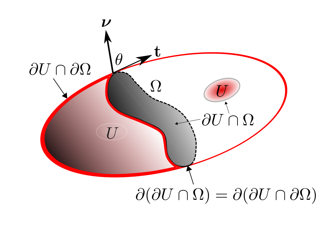
Figure 2: The geometry of the domain Ω\Omega and the interface ∂U∩Ω\partial U\cap\Omega

The existence of a minimizer for the limiting problem

inf𝐮∈𝒜0𝒢0​[𝐮]\inf_{\mathbf{u}\in\mathscr{A}_{0}}\mathcal{G}_{0}[\mathbf{u}]

is obtained through the standard direct method in the calculus of variations. By the straight forward calculation of the first variation, we get the following necessary condition for the interface.

Theorem 4.5.

Let Ω\Omega be a bounded domain with a C2C^{2}-boundary ∂Ω\partial\Omega and 𝐮0\mathbf{u}_{0} be a critical point of 𝒢0\mathcal{G}_{0} such that ∂U∩Ω\partial U\cap\Omega is of class 𝒞2\mathcal{C}^{2} with mean curvature H:∂U∩Ω→ℝH:\partial U\cap\Omega\to\mathbb{R}. The corresponding Euler-Lagrange equation of min⁡𝒢0​[𝐮]\min\mathcal{G}_{0}[\mathbf{u}] is

{H⁡(x)=Const.for ​x∈∂U∩Ω,g⁡(𝐚,𝐛)​(𝝂⋅𝐭)+g⁡(𝟎,𝐚)−g⁡(𝟎,𝐛)=0for ​x∈∂(∂U∩Ω)\left\{\begin{array}[]{ll}H(x)=\textrm{Const.}&\qquad\textrm{for }x\in\partial U\cap\Omega,\\ g(\mathbf{a},\mathbf{b})(\boldsymbol{\nu}\cdot\mathbf{t})+g(\mathbf{0},\mathbf{a})-g(\mathbf{0},\mathbf{b})=0&\qquad\textrm{for }x\in\partial(\partial U\cap\Omega)\end{array}\right.

where 𝛎:∂(∂U∩Ω)→𝕊n−1\boldsymbol{\nu}:\partial(\partial U\cap\Omega)\to\mathbb{S}^{n-1} is an outward unit tangential vector to the interface ∂U∩Ω\partial U\cap\Omega and normal to ∂(∂U∩Ω)\partial(\partial U\cap\Omega); 𝐭:∂(∂U∩Ω)→𝕊n−1\mathbf{t}:\partial(\partial U\cap\Omega)\to\mathbb{S}^{n-1} is the outward unit tangential vector to ∂U∩∂Ω\partial U\cap\partial\Omega and normal to ∂(∂U∩∂Ω)\partial(\partial U\cap\partial\Omega).

Proof.

The calculation the first variation of 𝒢0\mathcal{G}_{0} under the fixed volume constraint is similar to [15, 52]. We omit it here. ∎

Remark 4.1.

The second equation of the Euler-Lagrange equation is called the Young’s relation, which appears in natural process of wetting:

g⁡(𝐚,𝐛)​cos⁡θ+g⁡(𝟎,𝐚)−g⁡(𝟎,𝐛)=0.g(\mathbf{a},\mathbf{b})\cos\theta+g(\mathbf{0},\mathbf{a})-g(\mathbf{0},\mathbf{b})=0.

Here, the contact angle between the boundary and the interface is denoted by θ\theta, see Figure 2. Indeed, it is a balance law between surface tensions of three different interfaces on the boundary. Thus, the Euler-Lagrange equation mentioned above could also be considered as a equation for a quantum-like wetting process.

4.3 Preliminary lemmas

The function W:ℝ3→ℝW:\mathbb{R}^{3}\to\mathbb{R} constructed in those sections has the following properties:

  1. 1.

    WW is a C1C^{1}-nonnegative function with the following symmetry property:

    W⁡(u1,u0,u−1)=W⁡(−u1,u0,u−1)=W⁡(u1,−u0,u−1)=W⁡(u1,u0,−u−1)W(u_{1},u_{0},u_{-1})=W(-u_{1},u_{0},u_{-1})=W(u_{1},-u_{0},u_{-1})=W(u_{1},u_{0},-u_{-1}) (4.4)

    and

    W⁡(𝐮)=0​ in ​ℝ+3​ if and only if ​𝐮={𝐚,𝐛}.W(\mathbf{u})=0\textrm{ in }\mathbb{R}^{3}_{+}\ \textrm{ if and only if }\mathbf{u}=\{\mathbf{a},\mathbf{b}\}.
  2. 2.

    There exist δ>0\delta>0 and C>0C>0 such that

    C​|𝐮−𝐚|2≤W⁡(𝐮)≤1C​|𝐮−𝐚|2 for ​|𝐮−𝐚|<δC|\mathbf{u}-\mathbf{a}|^{2}\leq W(\mathbf{u})\leq\frac{1}{C}|\mathbf{u}-\mathbf{a}|^{2}\quad\textrm{ for }|\mathbf{u}-\mathbf{a}|<\delta (4.5)

    and

    C​|𝐮−𝐛|2≤W⁡(𝐮)≤1C​|𝐮−𝐛|2 for ​|𝐮−𝐛|<δ.C|\mathbf{u}-\mathbf{b}|^{2}\leq W(\mathbf{u})\leq\frac{1}{C}|\mathbf{u}-\mathbf{b}|^{2}\quad\textrm{ for }|\mathbf{u}-\mathbf{b}|<\delta. (4.6)
  3. 3.

    There exist two positive values CC and RR such that

    C​|𝐮|2≤W⁡(𝐮)for ​|𝐮|>R.C|\mathbf{u}|^{2}\leq W(\mathbf{u})\qquad\textrm{for }|\mathbf{u}|>R. (4.7)

We shall assume these properties of WW in the discussion below.

We quote several useful lemmas from [3, 43, 55, 56] which will be used in the proof of our Γ\Gamma-convergence result.

Lemma 4.6 (See [43, 55]).

Let Ω\Omega be an open bounded subset in ℝn\mathbb{R}^{n} with Lipschitz-continuous boundary. Let AA be an open subset in ℝn\mathbb{R}^{n} with compact C2C^{2}-boundary ∂A\partial A such that Hn−1​(∂A∩∂Ω)=0H^{n-1}(\partial A\cap\partial\Omega)=0. Define the signed distance function to ∂A\partial A, d:Ω→ℝd:\Omega\to\mathbb{R}, by

dA​(x)={dist​(x,∂A)x∈Ω\A,−dist​(x,∂A)x∈A∩Ω.d_{A}(x)=\left\{\begin{array}[]{rl}\textrm{dist}(x,\partial A)&x\in\Omega\backslash A,\\ -\textrm{dist}(x,\partial A)&x\in A\cap\Omega.\end{array}\right. (4.8)

Then for some s>0s>0, dd is C2C^{2} function in {|d(x)|<s}\{|d(x)|<s\} with

|∇dA|=1.|\nabla d_{A}|=1.

Furthermore,

lims→0ℋn−1​({x∈Ω:dA​(x)=s})=ℋn−1​(∂A∩Ω).\lim_{s\to 0}\mathcal{H}^{n-1}(\{x\in\Omega:\,d_{A}(x)=s\})=\mathcal{H}^{n-1}(\partial A\cap\Omega). (4.9)
Lemma 4.7 (See [3, 55, 56]).

For any 𝛏0,𝛏1∈ℝ+3\boldsymbol{\xi}_{0},\boldsymbol{\xi}_{1}\in\mathbb{R}^{3}_{+}, there exists a curve 𝛄𝛏0,𝛏1:[0,1]→ℝ+3\boldsymbol{\gamma}_{\boldsymbol{\xi}_{0},\boldsymbol{\xi}_{1}}:[0,1]\to\mathbb{R}^{3}_{+} with 𝛄⁡(0)=𝛏0\boldsymbol{\gamma}(0)=\boldsymbol{\xi}_{0} and 𝛄⁡(1)=𝛏1\boldsymbol{\gamma}(1)=\boldsymbol{\xi}_{1} which minimizes the degenerate geodesic problem

g(𝝃0,𝝃1):=inf{∫01W⁡(𝜸⁡(τ))|𝜸′(τ)|dτ:𝜸∈Lip([0,1];𝐑+3),𝜸(0)=𝝃0,𝜸(1)=𝝃1}.g(\boldsymbol{\xi}_{0},\boldsymbol{\xi}_{1}):=\inf\left\{\int_{0}^{1}\sqrt{W(\boldsymbol{\gamma}(\tau))}\,|\boldsymbol{\gamma}^{\prime}(\tau)|\,d\tau:\,\boldsymbol{\gamma}\in Lip([0,1];\mathbf{R}^{3}_{+}),\,\boldsymbol{\gamma}(0)=\boldsymbol{\xi}_{0},\,\boldsymbol{\gamma}(1)=\boldsymbol{\xi}_{1}\right\}.

Define φ𝛏0​(𝛏1)=g⁡(𝛏0,𝛏1)\varphi_{\boldsymbol{\xi}_{0}}(\boldsymbol{\xi}_{1})=g(\boldsymbol{\xi}_{0},\boldsymbol{\xi}_{1}). Then the function φ𝛏0:ℝ+3→ℝ+\varphi_{\boldsymbol{\xi}_{0}}:\mathbb{R}^{3}_{+}\to\mathbb{R}_{+} is Lipchitz-continuous with the property

|∇φ𝝃0​(𝝃1)|=W⁡(𝝃1) for almost all ​𝝃1∈ℝ+3.|\nabla\varphi_{\boldsymbol{\xi}_{0}}(\boldsymbol{\xi}_{1})|=\sqrt{W(\boldsymbol{\xi}_{1})}\quad\textrm{ for almost all }\boldsymbol{\xi}_{1}\in\mathbb{R}^{3}_{+}.

Furthermore, if 𝐮∈H1​(Ω,ℝ+3)∩L∞​(Ω,ℝ+3)\mathbf{u}\in H^{1}(\Omega;\mathbb{R}^{3}_{+})\cap L^{\infty}(\Omega;\mathbb{R}^{3}_{+}), then φ𝛏0∘𝐮∈W1,1​(Ω,ℝ+3)\varphi_{\boldsymbol{\xi}_{0}}\circ\mathbf{u}\in W^{1,1}(\Omega;\mathbb{R}^{3}_{+}) and

∫Ω|∇(φ𝝃0∘𝐮)|𝑑x≤∫ΩW⁡(𝐮⁡(x))​|∇𝐮​(x)|​𝑑x,\int_{\Omega}|\nabla(\varphi_{\boldsymbol{\xi}_{0}}\circ\mathbf{u})|\,dx\leq\int_{\Omega}\sqrt{W(\mathbf{u}(x))}|\nabla\mathbf{u}(x)|\,dx, (4.10)

where |∇𝐮||\nabla\mathbf{u}| is the 22-norm of ∇𝐮\nabla\mathbf{u}, that is

|∇𝐮|=(∑i,j=13(∂uj∂xi)2)1/2.|\nabla\mathbf{u}|=\left(\sum_{i,j=1}^{3}\left(\frac{\partial u_{j}}{\partial x_{i}}\right)^{2}\right)^{1/2}.
Proof.
  1. 1.

    This geodesic problem corresponds to a Riemannian metric d​s2=W​d​sE​u​c2ds^{2}=Wds_{Euc}^{2} on ℝ+3{\mathbb{R}}_{+}^{3}, where d​sE​u​cds_{Euc} is the Euclidean matric. However, there are two difficulties here. The first one is that this is a constrained variational problem, namely all components of the geodesic curve γ⁡(⋅)\mathscr{\gamma}(\cdot) should be non-negative. To resolve this difficulty, we extend this variational problem to the entire ℝ3\mathbb{R}^{3} by taking the advantage of the symmetry property of the function WW. Thus we consider an equivalent degenerate geodesic problem on ℝ3\mathbb{R}^{3}

    inf{∫01W⁡(𝜸⁡(τ))|𝜸′(τ)|dτ:𝜸∈Lip([0,1];ℝ3),𝜸(0)=𝝃0,𝜸(1)=𝝃1},\inf\left\{\int_{0}^{1}\sqrt{W(\boldsymbol{\gamma}(\tau))}\,|\boldsymbol{\gamma}^{\prime}(\tau)|\,d\tau:\,\boldsymbol{\gamma}\in Lip([0,1];\mathbb{R}^{3}),\,\boldsymbol{\gamma}(0)=\boldsymbol{\xi}_{0},\,\boldsymbol{\gamma}(1)=\boldsymbol{\xi}_{1}\right\}, (4.11)

    For any 𝝃0,𝝃1∈ℝ+3\boldsymbol{\xi}_{0},\boldsymbol{\xi}_{1}\in\mathbb{R}^{3}_{+}, if we have found a Lipschitz geodesic γ⁡(⋅)\mathscr{\gamma}(\cdot) connecting 𝝃0\boldsymbol{\xi}_{0} to 𝝃1\boldsymbol{\xi}_{1} in ℝ3{\mathbb{R}}^{3}, then using the symmetry property of WW and reflection, we can always find a representative Lipschitz-continuous curve 𝜸:[0,1]→ℝ+3\boldsymbol{\gamma}:[0,1]\to\mathbb{R}^{3}_{+} which solves the constrained geodesic problem.

  2. 2.

    The second difficuly is the degeneracy of W⁡(u)W(u) at 𝐚\mathbf{a} and 𝐛\mathbf{b}. Thus, the direct method in the calculus of variations cannot be applied straightforwardly. Therefore, we consider the regularized problem:

    inf{∫01(W⁡(𝜸⁡(τ))+δ)|𝜸′(τ)|dτ:𝜸∈Lip([0,1];ℝ3),𝜸(0)=𝝃0,𝜸(1)=𝝃1},\inf\left\{\int_{0}^{1}\left(\sqrt{W(\boldsymbol{\gamma}(\tau))+\delta}\right)\,|\boldsymbol{\gamma}^{\prime}(\tau)|\,d\tau:\,\boldsymbol{\gamma}\in Lip([0,1];\mathbb{R}^{3}),\,\boldsymbol{\gamma}(0)=\boldsymbol{\xi}_{0},\,\boldsymbol{\gamma}(1)=\boldsymbol{\xi}_{1}\right\}, (4.12)

    where δ>0\delta>0. The regularized Riemannian metric d​sδ2=(W+δ)​d​sE​u​c2ds_{\delta}^{2}=(W+\delta)ds_{Euc}^{2} is conformal to the Euclidean metric on the plane. Its minimizer 𝜸δ\boldsymbol{\gamma}_{\delta} exists uniquely by the direct method in the calculus of variations. A uniform bound on the Euclidean arclength ℓδ\ell_{\delta} of 𝜸δ\boldsymbol{\gamma}_{\delta} can be derived by carefully analyzing the curve 𝜸δ\boldsymbol{\gamma}_{\delta} in two different regions: one region is away from the zeros of WW and the other is the region near the zeros of WW. Because the value ℓδ\ell_{\delta} is invariant under re-parametrization of the curve 𝜸δ\boldsymbol{\gamma}_{\delta}, this allows us to choose a new parametrization 𝜸~δ:[0,1]→ℝ3\tilde{\boldsymbol{\gamma}}_{\delta}:[0,1]\to\mathbb{R}^{3} with a constant speed, that is |𝜸~δ′|≡ℓδ|\tilde{\boldsymbol{\gamma}}_{\delta}^{\prime}|\equiv\ell_{\delta}. By the Arzelá-Ascoli compactness theorem, there exists a subsequence {𝜸~δk}\{\tilde{\boldsymbol{\gamma}}_{\delta_{k}}\} and a curve 𝜸\boldsymbol{\gamma} such that 𝜸~δk\tilde{\boldsymbol{\gamma}}_{\delta_{k}} converges to 𝜸\boldsymbol{\gamma} in C⁡([0,1],ℝ3)C([0,1],{\mathbb{R}}^{3}). It is easy to see that 𝜸\boldsymbol{\gamma} solves the problem (4.11).

  3. 3.

    It is observed that g:ℝ+3×ℝ+3→ℝg:{\mathbb{R}}^{3}_{+}\times{\mathbb{R}}^{3}_{+}\to{\mathbb{R}} is a metric in ℝ+3{\mathbb{R}}^{3}_{+} and satisfies the triangle inequality:

    g⁡(𝝃0,𝝃1)≤g⁡(𝝃0,𝝃1′)+g⁡(𝝃1′,𝝃1).g(\boldsymbol{\xi}_{0},\boldsymbol{\xi}_{1})\leq g(\boldsymbol{\xi}_{0},\boldsymbol{\xi}_{1}^{\prime})+g(\boldsymbol{\xi}_{1}^{\prime},\boldsymbol{\xi}_{1}).

    That is,

    φ𝝃0​(𝝃1)−φ𝝃0​(𝝃1′)≤g⁡(𝝃1,𝝃1′)=∫01W​(𝜸𝝃1′,𝝃1​(τ))​|𝜸𝝃1′,𝝃1′​(τ)|​𝑑τ.\varphi_{\boldsymbol{\xi}_{0}}(\boldsymbol{\xi}_{1})-\varphi_{\boldsymbol{\xi}_{0}}(\boldsymbol{\xi}_{1}^{\prime})\leq g(\boldsymbol{\xi}_{1},\boldsymbol{\xi}_{1}^{\prime})=\int_{0}^{1}\sqrt{W(\boldsymbol{\gamma}_{\boldsymbol{\xi}_{1}^{\prime},\boldsymbol{\xi}_{1}}(\tau))}|\boldsymbol{\gamma}_{\boldsymbol{\xi}_{1}^{\prime},\boldsymbol{\xi}_{1}}^{\prime}(\tau)|\,d\tau. (4.13)

    From this, we get that φ𝝃0\varphi_{\boldsymbol{\xi}_{0}} is locally Lipchitz continuous and

    |∇φ𝝃0​(𝝃1)|≤W⁡(𝝃1)|\nabla\varphi_{\boldsymbol{\xi}_{0}}(\boldsymbol{\xi}_{1})|\leq\sqrt{W(\boldsymbol{\xi}_{1})} (4.14)

    As we choose 𝝃1′\boldsymbol{\xi}_{1}^{\prime} moving along the geodesic 𝜸𝝃0,𝝃1\boldsymbol{\gamma}_{\boldsymbol{\xi}_{0},\boldsymbol{\xi}_{1}} to approach 𝝃1\boldsymbol{\xi}_{1}, then the inequality in (4.13) becomes equality, and we get

    |∇φ𝝃0​(𝝃1)|=W⁡(𝝃1).|\nabla\varphi_{\boldsymbol{\xi}_{0}}(\boldsymbol{\xi}_{1})|=\sqrt{W(\boldsymbol{\xi}_{1})}. (4.15)

    Notice that the above arguments hold for all 𝝃1\boldsymbol{\xi}_{1} in the interior of ℝ+3{\mathbb{R}}_{+}^{3}. But the inequality (4.14) and equality (4.15) can be extended to the boundary of ℝ+3{\mathbb{R}}_{+}^{3}.

  4. 4.

    Applying the Cauchy inequality and from (4.14), we get

    ∫Ω|∇(φ𝝃0∘𝐮)|​dx=\displaystyle\int_{\Omega}|\nabla(\varphi_{\boldsymbol{\xi}_{0}}\circ\mathbf{u})|\,dx= ∫Ω|(∇φ𝝃0​(𝐮))​∇x𝐮|​𝑑x\displaystyle\int_{\Omega}\left|\left(\nabla\varphi_{\boldsymbol{\xi}_{0}}(\mathbf{u})\right)\nabla_{x}\mathbf{u}\right|\,dx
    ≤\displaystyle\leq ∫Ω|∇φ𝝃0​(𝐮)|​|∇x𝐮|​dx≤\displaystyle\int_{\Omega}\left|\nabla\varphi_{\boldsymbol{\xi}_{0}}(\mathbf{u})\right|\left|\nabla_{x}\mathbf{u}\right|\,dx\leq ∫ΩW⁡(𝐮⁡(x))​|∇𝐮​(x)|​𝑑x\displaystyle\int_{\Omega}\sqrt{W(\mathbf{u}(x))}|\nabla\mathbf{u}(x)|\,dx

    for 𝐮∈C1​(Ω,ℝ+3)\mathbf{u}\in C^{1}(\Omega;\mathbb{R}^{3}_{+}). By the density theorem, this inequality also holds for 𝐮∈H1​(Ω,ℝ+3)∩L∞​(Ω,ℝ+3)\mathbf{u}\in H^{1}(\Omega;\mathbb{R}_{+}^{3})\cap L^{\infty}(\Omega;\mathbb{R}_{+}^{3}).

∎

The following lemma is used to construct the one-dimensional profile of the internal layer.

Lemma 4.8 (See [55, 56]).

Given 𝐚,𝐛∈ℝ+3\mathbf{a},\mathbf{b}\in{\mathbb{R}}_{+}^{3}. Then there exists a Lipchitz-continuous function 𝛈:(−∞,∞)→ℝ+3\boldsymbol{\eta}:(-\infty,\infty)\to\mathbb{R}^{3}_{+} whose trajectory is the geodesic with the metric d​s2=W​d​sE​u​c2ds^{2}=Wds^{2}_{Euc} connecting 𝐚\mathbf{a} to 𝐛\mathbf{b}. The function 𝛈⁡(⋅)\boldsymbol{\eta}(\cdot) solves the variational problem

inf𝜼⁡(−∞)=𝐚𝜼⁡(+∞)=𝐛∫−∞∞|𝜼′|2+W⁡(𝜼)​𝑑s\inf_{\begin{subarray}{c}\boldsymbol{\eta}(-\infty)=\mathbf{a}\\ \boldsymbol{\eta}(+\infty)=\mathbf{b}\end{subarray}}\int_{-\infty}^{\infty}|\boldsymbol{\eta}^{\prime}|^{2}+W(\boldsymbol{\eta})\,ds

with minimal value 2​g​(𝐚,𝐛)2g(\mathbf{a},\mathbf{b}) and

|𝜼⁡(t)−𝐚|<C​ec1​tas ​t→−∞,|\boldsymbol{\eta}(t)-\mathbf{a}|<Ce^{c_{1}t}\qquad\textrm{as }t\to-\infty, (4.16)
|𝜼⁡(t)−𝐛|<C​e−c1​tas ​t→+∞.|\boldsymbol{\eta}(t)-\mathbf{b}|<Ce^{-c_{1}t}\qquad\textrm{as }t\to+\infty. (4.17)
Proof.

Let 𝜸⁡(⋅)\boldsymbol{\gamma}(\cdot) be the geodesic curve in Lemma 4.7 connecting 𝐚\mathbf{a} to 𝐛\mathbf{b}. Let us parametrize it by β∈[0,1]\beta\in[0,1] such that 𝜸⁡(0)=𝐚\boldsymbol{\gamma}(0)=\mathbf{a}, 𝜸⁡(1)=𝐛\boldsymbol{\gamma}(1)=\mathbf{b}, 𝜸⁡(⋅)\boldsymbol{\gamma}(\cdot) is Lipschitz continuous and |𝜸′​(β)|≥c>0|\boldsymbol{\gamma}^{\prime}(\beta)|\geq c>0 for some constant cc and for all β∈[0,1]\beta\in[0,1]. Now, let us consider the ODE:

{d​βd​t​(t)=W⁡(𝜸⁡(β))|𝜸′​(β)|,β⁡(0)=12.\left\{\begin{array}[]{rcl}\frac{d\beta}{dt}(t)&=&\frac{\sqrt{W(\boldsymbol{\gamma}(\beta))}}{|\boldsymbol{\gamma}^{\prime}(\beta)|},\\ \beta(0)&=&\frac{1}{2}.\end{array}\right.

The right-hand side of this ODE, f⁡(β):=W⁡(𝜸⁡(β))/|𝜸′​(β)|f(\beta):=\sqrt{W(\boldsymbol{\gamma}(\beta))}/|\boldsymbol{\gamma}^{\prime}(\beta)|, is Lipchiptz continuous on [0,1][0,1], thus we have local existence and uniqueness of the solution. Note that β=0,1\beta=0,1 are the only two zeros of ff, thus, from uniqueness, the solution of this ODE stays between 00 and 11, as long as it exists. Thereby it exists globally. Furthermore, β⁡(t)→0\beta(t)\to 0 (resp. β⁡(t)→1\beta(t)\to 1) exponentially fast as t→−∞t\to-\infty (resp. t→∞t\to\infty) because f′​(0)f^{\prime}(0) (resp. f′​(1)≠0f^{\prime}(1)\neq 0), which is, in turn, due to (4.5) (resp. (4.6)).

Now let us define 𝜼⁡(t):=𝜸⁡(β⁡(t))\boldsymbol{\eta}(t):=\boldsymbol{\gamma}(\beta(t)). We have

|𝜼′​(t)|=|𝜸′​(β⁡(t))​β′​(t)|=|𝜸′​(β⁡(t))|​β′​(t)=W⁡(𝜸⁡(β⁡(t)))=W⁡(𝜼⁡(t)).|\boldsymbol{\eta}^{\prime}(t)|=|\boldsymbol{\gamma}^{\prime}(\beta(t))\beta^{\prime}(t)|=|\boldsymbol{\gamma}^{\prime}(\beta(t))|\beta^{\prime}(t)=\sqrt{W(\boldsymbol{\gamma}(\beta(t)))}=\sqrt{W(\boldsymbol{\eta}(t))}.

Let 𝜼^∈L​i​p​((−∞,∞),ℝ+3)\hat{\boldsymbol{\eta}}\in Lip((-\infty,\infty),{\mathbb{R}}_{+}^{3}) be any curve connecting 𝐚\mathbf{a} to 𝐛\mathbf{b}. Using the Cauchy inequality, the fact that 𝜸\boldsymbol{\gamma} is geodesic and |𝜼′|=W⁡(𝜼)|\boldsymbol{\eta}^{\prime}|=W(\boldsymbol{\eta}), we get

∫−∞∞|𝜼^′|2+W⁡(𝜼^)​𝑑t≥2​∫−∞∞W⁡(𝜼^)​|𝜼^′|​𝑑t≥2​∫−∞∞W⁡(𝜼)|𝜼′|𝑑t=∫−∞∞|𝜼′|2+W⁡(𝜼)​𝑑t\int_{-\infty}^{\infty}|\hat{\boldsymbol{\eta}}^{\prime}|^{2}+W(\hat{\boldsymbol{\eta}})\,dt\geq 2\int_{-\infty}^{\infty}\sqrt{W(\hat{\boldsymbol{\eta}})}{|\hat{\boldsymbol{\eta}}^{\prime}|}\,dt\geq 2\int_{-\infty}^{\infty}\sqrt{W(\boldsymbol{\eta})}{|\boldsymbol{\eta}^{\prime}|}\,dt=\int_{-\infty}^{\infty}|\boldsymbol{\eta}^{\prime}|^{2}+W(\boldsymbol{\eta})\,dt

Thus, 𝜼\boldsymbol{\eta} solves the variational problem. ∎

Similarly, we also have the lemma for the construction of the one-dimensional profile of the boundary layer due to the difference between the Dirichlet boundary condition 𝐮=𝟎\mathbf{u}=\mathbf{0} on ∂Ω\partial\Omega and 𝐮=𝐚,𝐛\mathbf{u}=\mathbf{a},\,\mathbf{b} in Ω\Omega.

Lemma 4.9.

There exist two Lipchitz-continuous functions 𝛈𝐚:(0,∞)→ℝ+3\boldsymbol{\eta}_{\mathbf{a}}:(0,\infty)\to\mathbb{R}^{3}_{+} and 𝛈𝐛:(0,∞)→ℝ+3\boldsymbol{\eta}_{\mathbf{b}}:(0,\infty)\to\mathbb{R}^{3}_{+}, whose trajectories are the geodesics with the metric d​s2=W​d​sE​u​c2ds^{2}=Wds^{2}_{Euc} connecting 𝟎\mathbf{0} to 𝐚\mathbf{a} and to 𝐛\mathbf{b}, respectively. They solve the variational problems

inf𝜼⁡(0)=𝟎𝜼⁡(+∞)=𝐚∫0∞|𝜼′|2+W⁡(𝜼)​𝑑t\inf_{\begin{subarray}{c}\boldsymbol{\eta}(0)=\mathbf{0}\\ \boldsymbol{\eta}(+\infty)=\mathbf{a}\end{subarray}}\int_{0}^{\infty}|\boldsymbol{\eta}^{\prime}|^{2}+W(\boldsymbol{\eta})\,dt

and

inf𝜼⁡(0)=𝟎𝜼⁡(+∞)=𝐛∫0∞|𝜼′|2+W⁡(𝜼)​𝑑t,\inf_{\begin{subarray}{c}\boldsymbol{\eta}(0)=\mathbf{0}\\ \boldsymbol{\eta}(+\infty)=\mathbf{b}\end{subarray}}\int_{0}^{\infty}|\boldsymbol{\eta}^{\prime}|^{2}+W(\boldsymbol{\eta})\,dt,

with minimal values 2​g​(𝟎,𝐚)2g(\mathbf{0},\mathbf{a}) and 2​g​(𝟎,𝐛)2g(\mathbf{0},\mathbf{b}), respectively. Furthermore, limt→+∞𝛈𝐚​(t)=𝐚\lim_{t\to+\infty}\boldsymbol{\eta}_{\mathbf{a}}(t)=\mathbf{a} and limt→+∞𝛈𝐛​(t)=𝐛\lim_{t\to+\infty}\boldsymbol{\eta}_{\mathbf{b}}(t)=\mathbf{b} are being attained at exponential rates.

Proof.

The proof is similar to the proof of Lemma 4.8. ∎

4.4 Proofs of the Main Theorems

Proof of Theorem 4.1

Proof of Lower semi-continuity.

1. Let us extend 𝐮ϵ\mathbf{u}_{\epsilon} and 𝐮0\mathbf{u}_{0} trivially to a larger bounded smooth domain Ω′\Omega^{\prime} such that Ω¯⊂⊂Ω′\overline{\Omega}\subset\subset\Omega^{\prime}. That is,

𝐮~ϵ​(x)={𝐮ϵ​(x)for ​x∈Ω,𝟎for ​x∈Ω′\Ω,and𝐮~0​(x)={𝐮0​(x)for ​x∈Ω,𝟎for ​x∈Ω′\Ω.\tilde{\mathbf{u}}_{\epsilon}(x)=\left\{\begin{array}[]{ll}\mathbf{u}_{\epsilon}(x)&\quad\textrm{for }x\in\Omega,\\ \mathbf{0}&\quad\textrm{for }x\in\Omega^{\prime}\backslash\Omega,\end{array}\right.\qquad\textrm{and}\qquad\tilde{\mathbf{u}}_{0}(x)=\left\{\begin{array}[]{ll}\mathbf{u}_{0}(x)&\quad\textrm{for }x\in\Omega,\\ \mathbf{0}&\quad\textrm{for }x\in\Omega^{\prime}\backslash\Omega.\end{array}\right.

We have 𝐮~ϵ→𝐮~0\tilde{\mathbf{u}}_{\epsilon}\to\tilde{\mathbf{u}}_{0} in (L2​(Ω′))3(L^{2}(\Omega^{\prime}))^{3}. This together with the fact that the two functions φ𝐚\varphi_{\mathbf{a}} and φ𝟎\varphi_{\mathbf{0}} are Lipschitz continuous ( Lemma 4.7) lead to

(φ𝐚∘𝐮~ϵ)​(x)→(φ𝐚∘𝐮~0)​(x)={0x∈Ug⁡(𝐚,𝐛)x∈Ω\Ug⁡(𝐚,𝟎)x∈Ω′\Ωin ​L2​(Ω′)(\varphi_{\mathbf{a}}\circ\tilde{\mathbf{u}}_{\epsilon})(x)\to(\varphi_{\mathbf{a}}\circ\tilde{\mathbf{u}}_{0})(x)=\left\{\begin{array}[]{ll}0&\quad x\in U\\ g(\mathbf{a},\mathbf{b})&\quad x\in\Omega\backslash U\\ g(\mathbf{a},\mathbf{0})&\quad x\in\Omega^{\prime}\backslash\Omega\end{array}\right.\quad\textrm{in }L^{2}(\Omega^{\prime})

and

(φ𝟎∘𝐮~ϵ)​(x)→(φ𝟎∘𝐮~0)​(x)={g⁡(𝟎,𝐚)x∈Ug⁡(𝟎,𝐛)x∈Ω\U0x∈Ω′\Ωin ​L2​(Ω′).(\varphi_{\mathbf{0}}\circ\tilde{\mathbf{u}}_{\epsilon})(x)\to(\varphi_{\mathbf{0}}\circ\tilde{\mathbf{u}}_{0})(x)=\left\{\begin{array}[]{ll}g(\mathbf{0},\mathbf{a})&\quad x\in U\\ g(\mathbf{0},\mathbf{b})&\quad x\in\Omega\backslash U\\ 0&\quad x\in\Omega^{\prime}\backslash\Omega\end{array}\right.\quad\textrm{in }L^{2}(\Omega^{\prime}).

2. Let Λ1δ\Lambda_{1}^{\delta} and Λ2δ\Lambda_{2}^{\delta} be two bounded sets defined by

Λ1δ={x∈Ω:dist​(x,∂Ω)≥δ}andΛ2δ={x∈Ω:dist​(x,∂Ω)<δ}∪(Ω′\Ω).\Lambda_{1}^{\delta}=\{x\in\Omega:\textrm{dist}(x,\partial\Omega)\geq\delta\}\quad\textrm{and}\quad\Lambda_{2}^{\delta}=\{x\in\Omega:\textrm{dist}(x,\partial\Omega)<\delta\}\cup(\Omega^{\prime}\backslash\Omega).

By using the inequality of arithmetic and geometric means and the lower semicontinuity of the BV-norm under L1L^{1}-convergence, we have

lim infϵ→0𝒢ϵ​[𝐮ϵ]≥2​lim infϵ→0∫ΩW​(𝐮ϵ​(x))​|∇𝐮ϵ​(x)|​𝑑x\displaystyle\liminf_{\epsilon\to 0}\mathcal{G}_{\epsilon}[\mathbf{u}_{\epsilon}]\geq 2\liminf_{\epsilon\to 0}\int_{\Omega}\sqrt{W(\mathbf{u}_{\epsilon}(x))}\,|\nabla\mathbf{u}_{\epsilon}(x)|\,dx
=2​lim infϵ→0(∫Λ1δW​(𝐮~ϵ​(x))​|∇𝐮~ϵ​(x)|​𝑑x+∫Λ2δW​(𝐮~ϵ​(x))​|∇𝐮~ϵ​(x)|​𝑑x)\displaystyle=2\liminf_{\epsilon\to 0}\left(\int_{\Lambda_{1}^{\delta}}\sqrt{W(\tilde{\mathbf{u}}_{\epsilon}(x))}\,|\nabla\tilde{\mathbf{u}}_{\epsilon}(x)|\,dx+\int_{\Lambda_{2}^{\delta}}\sqrt{W(\tilde{\mathbf{u}}_{\epsilon}(x))}\,|\nabla\tilde{\mathbf{u}}_{\epsilon}(x)|\,dx\right)
≥2​lim infϵ→0∫Λ1δW​(𝐮~ϵ​(x))|∇𝐮~ϵ​(x)|𝑑x+2​lim infϵ→0∫Λ2δW​(𝐮~ϵ​(x))​|∇𝐮~ϵ​(x)|​𝑑x\displaystyle\geq 2\liminf_{\epsilon\to 0}\int_{\Lambda_{1}^{\delta}}\sqrt{W(\tilde{\mathbf{u}}_{\epsilon}(x))}\,|\nabla\tilde{\mathbf{u}}_{\epsilon}(x)|\,dx+2\liminf_{\epsilon\to 0}\int_{\Lambda_{2}^{\delta}}\sqrt{W(\tilde{\mathbf{u}}_{\epsilon}(x))}\,|\nabla\tilde{\mathbf{u}}_{\epsilon}(x)|\,dx

After applying the inequality (4.10) to the function φ𝐚∘𝐮~ϵ\varphi_{\mathbf{a}}\circ\tilde{\mathbf{u}}_{\epsilon} on the domain Λ1δ\Lambda_{1}^{\delta} and the function φ𝟎∘𝐮~ϵ\varphi_{\mathbf{0}}\circ\tilde{\mathbf{u}}_{\epsilon} on the domain Λ2δ\Lambda_{2}^{\delta}, we find that

lim infϵ→0𝒢ϵ​[𝐮ϵ]\displaystyle\liminf_{\epsilon\to 0}\mathcal{G}_{\epsilon}[\mathbf{u}_{\epsilon}] ≥2​lim infϵ→0∫Λ1δ|∇(φ𝐚∘𝐮~ϵ)|​𝑑x+2​lim infϵ→0∫Λ2δ|∇(φ𝟎∘𝐮~ϵ)|​𝑑x\displaystyle\geq 2\liminf_{\epsilon\to 0}\int_{\Lambda_{1}^{\delta}}|\nabla(\varphi_{\mathbf{a}}\circ\tilde{\mathbf{u}}_{\epsilon})|\,dx+2\liminf_{\epsilon\to 0}\int_{\Lambda_{2}^{\delta}}|\nabla(\varphi_{\mathbf{0}}\circ\tilde{\mathbf{u}}_{\epsilon})|\,dx
≥2​(∫Λ1δ|∇(φ𝐚∘𝐮~0)|+∫Λ2δ|∇(φ𝟎∘𝐮~0)|).\displaystyle\geq 2\left(\int_{\Lambda_{1}^{\delta}}|\nabla(\varphi_{\mathbf{a}}\circ\tilde{\mathbf{u}}_{0})|+\int_{\Lambda_{2}^{\delta}}|\nabla(\varphi_{\mathbf{0}}\circ\tilde{\mathbf{u}}_{0})|\right).

Taking δ→0\delta\to 0, we get

lim infϵ→0𝒢ϵ​[𝐮ϵ]\displaystyle\liminf_{\epsilon\to 0}\mathcal{G}_{\epsilon}[\mathbf{u}_{\epsilon}] ≥2​g​(𝐚,𝐛)​PerΩ​(𝐮=𝐚)+2​g​(𝟎,𝐚)​ℋ2​({x∈∂Ω:𝐮=a})\displaystyle\geq 2g(\mathbf{a},\mathbf{b})\,\textrm{Per}_{\Omega}(\mathbf{u}=\mathbf{a})+2g(\mathbf{0},\mathbf{a})\,\mathcal{H}^{2}(\{x\in\partial\Omega:\mathbf{u}=a\})
+2​g​(𝟎,𝐛)​ℋ2​({x∈∂Ω:𝐮=b}).\displaystyle\qquad+2g(\mathbf{0},\mathbf{b})\,\mathcal{H}^{2}(\{x\in\partial\Omega:\mathbf{u}=b\}).

□\Box

Proof of Recovery sequence.
1. We will construct recovery sequence {𝐯ϵ}⊂𝒜\{\mathbf{v}_{\epsilon}\}\subset\mathscr{A} for 𝐯0∈𝒜0\mathbf{v}_{0}\in\mathscr{A}_{0} (4.1) of the form

𝐯0={𝐚if ​x∈V,𝐛if ​x∈Ω\V,\mathbf{v}_{0}=\left\{\begin{array}[]{ll}\mathbf{a}&\qquad\textrm{if }x\in V,\\ \mathbf{b}&\qquad\textrm{if }x\in\Omega\backslash V,\end{array}\right. (4.18)

and satisfies 𝒩⁡[𝐯0]=N,ℳ⁡[𝐯0]=M\mathcal{N}[\mathbf{v}_{0}]=N,\mathcal{M}[\mathbf{v}_{0}]=M. We discuss the case when 𝐯0∈𝒜0∩(B​V​(Ω))3\mathbf{v}_{0}\in\mathscr{A}_{0}\cap(BV(\Omega))^{3} first. The case when 𝐯0∈𝒜0∖(B​V​(Ω))3\mathbf{v}_{0}\in\mathscr{A}_{0}\setminus(BV(\Omega))^{3} will be discussed in item 6 below. In the first case, since 𝐯0∈(B​V​(Ω))3\mathbf{v}_{0}\in(BV(\Omega))^{3}, the set VV has finite perimeter in Ω\Omega. We may assume that the interface Γ=∂V∩Ω\Gamma=\partial V\cap\Omega is smooth because a set of finite perimeter can be approximated by a sequence of sets with smooth boundary, see [55].

2. The recovery sequence 𝐯ϵ\mathbf{v}_{\epsilon} to be constructed will have the form

𝐯ϵ​(x)=𝐰ϵ​(x)+α1​(ϵ)​𝝋​(x)+α2​(ϵ)​𝝍​(x).\mathbf{v}_{\epsilon}(x)=\mathbf{w}_{\epsilon}(x)+\alpha_{1}(\epsilon)\,\boldsymbol{\varphi}(x)+\alpha_{2}(\epsilon)\,\boldsymbol{\psi}(x).

Here, 𝐰ϵ\mathbf{w}_{\epsilon} is a layer solution; 𝝋⁡(x)\boldsymbol{\varphi}(x), 𝝍⁡(x)\boldsymbol{\psi}(x) are smooth functions supported on VV and Ω∖V\Omega\setminus V, respectively; the coefficients α1​(ϵ),α2​(ϵ)\alpha_{1}(\epsilon),\alpha_{2}(\epsilon) are O⁡(ϵ)O(\epsilon). The terms α1​(ϵ)​𝝋​(x)+α2​(ϵ)​𝝍​(x)\alpha_{1}(\epsilon)\,\boldsymbol{\varphi}(x)+\alpha_{2}(\epsilon)\,\boldsymbol{\psi}(x) are designed so that the conservation constraints 𝒩⁡[𝐯ϵ]=N\mathcal{N}[\mathbf{v}_{\epsilon}]=N and ℳ⁡[𝐯ϵ]=M\mathcal{M}[\mathbf{v}_{\epsilon}]=M are satisfied. Detail conditions for 𝝋⁡(x)\boldsymbol{\varphi}(x) and 𝝍⁡(x)\boldsymbol{\psi}(x) will be given later. The layer solution 𝐰ϵ\mathbf{w}_{\epsilon} involves an internal layer function 𝜼\boldsymbol{\eta} and an auxiliary boundary layer function 𝜼~\tilde{\boldsymbol{\eta}}. The internal layer function 𝜼\boldsymbol{\eta} is defined in Lemma 4.8, which connects 𝐚\mathbf{a} to 𝐛\mathbf{b}. The auxiliary boundary layer function 𝜼~:(−∞,∞)→ℝ+3\tilde{\boldsymbol{\eta}}:(-\infty,\infty)\to\mathbb{R}^{3}_{+} is defined by

𝜼~​(t)={𝜼𝐚​(−t)if ​t<0,𝜼𝐛​(t)if ​t≥0,\tilde{\boldsymbol{\eta}}(t)=\left\{\begin{array}[]{ll}\boldsymbol{\eta}_{\mathbf{a}}(-t)&\qquad\textrm{if }t<0,\\ \boldsymbol{\eta}_{\mathbf{b}}(t)&\qquad\textrm{if }t\geq 0,\end{array}\right.

where 𝜼𝐚\boldsymbol{\eta}_{\mathbf{a}} and 𝜼𝐛\boldsymbol{\eta}_{\mathbf{b}} are defined in Lemma 4.9. They are the boundary layer functions connecting 𝟎\mathbf{0} to 𝐚\mathbf{a} and to 𝐛\mathbf{b}, respectively. Note that the function 𝜼~​(t)\tilde{\boldsymbol{\eta}}(t) on the negative (resp. positive) half line {t<0}\{t<0\} (resp. {t>0}\{t>0\}) is the profile of the boundary layer approaching to the value 𝐚\mathbf{a} (resp. OPEN𝐛)\mathbf{b}). Let us also define the signed distance function d=dVd=d_{V} associated with ∂V{\partial}V by (4.8) and an auxiliary distance function associated with ∂Ω{\partial}\Omega by

db​(x)={−dist​(x,∂Ω) if ​x∈V,dist​(x,∂Ω) if ​x∈Ω∖V.d_{b}(x)=\left\{\begin{array}[]{ll}-\textrm{dist}(x,{\partial}\Omega)&\mbox{ if }x\in V,\\ \textrm{dist}(x,{\partial}\Omega)&\mbox{ if }x\in\Omega\setminus V.\end{array}\right.

We choose a cut-off function ζ\zeta, which is a smooth function such that 0≤ζ≤10\leq\zeta\leq 1 and

ζ⁡(t)={1if ​|t|≤1,0if ​|t|≥2.\zeta(t)=\left\{\begin{array}[]{ll}1&\qquad\textrm{if }|t|\leq 1,\\ 0&\qquad\textrm{if }|t|\geq 2.\end{array}\right.

Let us set γ=23\gamma=\frac{2}{3}. Finally, we define the layer solution 𝐰ϵ\mathbf{w}_{\epsilon} by

𝐰ϵ​(x)\displaystyle\mathbf{w}_{\epsilon}(x) =[1−ζ⁡(db​(x)ϵγ)]​{ζ⁡(d⁡(x)ϵγ)​𝜼​(d⁡(x)ϵ)+[1−ζ⁡(d⁡(x)ϵγ)]​𝐯0​(x)}\displaystyle=\left[1-\zeta\left(\frac{d_{b}(x)}{\epsilon^{\gamma}}\right)\right]\left\{\zeta\left(\frac{d(x)}{\epsilon^{\gamma}}\right)\boldsymbol{\eta}\left(\frac{d(x)}{\epsilon}\right)+\left[1-\zeta\left(\frac{d(x)}{\epsilon^{\gamma}}\right)\right]\mathbf{v}_{0}(x)\right\}
+ζ⁡(db​(x)ϵγ)​[1−ζ⁡(d⁡(x)ϵγ)]​𝜼~​(db​(x)ϵ).\displaystyle\qquad+\zeta\left(\frac{d_{b}(x)}{\epsilon^{\gamma}}\right)\left[1-\zeta\left(\frac{d(x)}{\epsilon^{\gamma}}\right)\right]\tilde{\boldsymbol{\eta}}\left(\frac{d_{b}(x)}{\epsilon}\right).
Figure 3: The domain represents the domain Ω\Omega ad the region on the left side of the solid line ∂V∩Ω\partial V\cap\Omega represents the domain VV. The distance between each type of line is ϵγ\epsilon^{\gamma}. The kk-region represents the sub-domain Ωk\Omega_{k}.

3. We claim that the sequence {𝐰ϵ}\{\mathbf{w}_{\epsilon}\} converges to 𝐯0\mathbf{v}_{0} in (L2​(Ω))3\left(L^{2}(\Omega)\right)^{3} and

𝒩⁡[𝐰ϵ]=N+nϵ,ℳ⁡[𝐰ϵ]=M+mϵ{\mathcal{N}}[\mathbf{w}_{\epsilon}]=N+n_{\epsilon},\qquad{\mathcal{M}}[\mathbf{w}_{\epsilon}]=M+m_{\epsilon} (4.19)

with nϵ=O⁡(ϵ)n_{\epsilon}=O(\epsilon) and mϵ=O⁡(ϵ)m_{\epsilon}=O(\epsilon).

We partition the domain Ω\Omega into sub-domains Ωk\Omega_{k} (See Figure 3):

Ω1\displaystyle\Omega_{1} ={x∈Ω:|d⁡(x)|​<ϵγ,|db​(x)|>​2​ϵγ},\displaystyle=\{x\in\Omega:|d(x)|<\epsilon^{\gamma},|d_{b}(x)|>2\epsilon^{\gamma}\},
Ω2\displaystyle\Omega_{2} ={x∈Ω:ϵγ≤|d(x)|≤2ϵγ,|db(x)|>2ϵγ},\displaystyle=\{x\in\Omega:\epsilon^{\gamma}\leq|d(x)|\leq 2\epsilon^{\gamma},|d_{b}(x)|>2\epsilon^{\gamma}\},
Ω3\displaystyle\Omega_{3} ={x∈Ω:|d(x)|>2ϵγ,|db(x)|<ϵγ},\displaystyle=\{x\in\Omega:|d(x)|>2\epsilon^{\gamma},|d_{b}(x)|<\epsilon^{\gamma}\},
Ω4\displaystyle\Omega_{4} ={x∈Ω:|d(x)|>2ϵγ,ϵγ≤|db(x)|≤2ϵγ},\displaystyle=\{x\in\Omega:|d(x)|>2\epsilon^{\gamma},\epsilon^{\gamma}\leq|d_{b}(x)|\leq 2\epsilon^{\gamma}\},
Ω5\displaystyle\Omega_{5} ={x∈Ω:|d(x)|>2ϵγ,|db(x)|>2ϵγ},\displaystyle=\{x\in\Omega:|d(x)|>2\epsilon^{\gamma},|d_{b}(x)|>2\epsilon^{\gamma}\},
Ω6\displaystyle\Omega_{6} ={x∈Ω:|d(x)|<2ϵγ,|db(x)|<2ϵγ}\displaystyle=\{x\in\Omega:|d(x)|<2\epsilon^{\gamma},|d_{b}(x)|<2\epsilon^{\gamma}\}

and estimate the following integral term by term on each subdomain Ωk\Omega_{k}:

∫Ω|𝐰ϵ−𝐯0|​𝑑x=∑k=16∫Ωk|𝐰ϵ−𝐯0|​𝑑x.\int_{\Omega}|\mathbf{w}_{\epsilon}-\mathbf{v}_{0}|\,dx=\sum_{k=1}^{6}\int_{\Omega_{k}}|\mathbf{w}_{\epsilon}-\mathbf{v}_{0}|\,dx.

We calculate

∫{x∈Ω1∪Ω2: 0<d⁡(x)<2​ϵγ}|𝐰ϵ−𝐯0|dx\displaystyle\int_{\{x\in\Omega_{1}\cup\Omega_{2}:\,0<d(x)<2\epsilon^{\gamma}\}}|\mathbf{w}_{\epsilon}-\mathbf{v}_{0}|\,dx ≤\displaystyle\leq ∫{0<d(x)<2ϵγ}|ζ(d⁡(x)ϵγ)(𝜼(d⁡(x)ϵ)−𝐛)|dx\displaystyle\int_{\{0<d(x)<2\epsilon^{\gamma}\}}\left|\zeta(\frac{d(x)}{\epsilon^{\gamma}})\left(\boldsymbol{\eta}(\frac{d(x)}{\epsilon})-\mathbf{b}\right)\right|\,dx
≤\displaystyle\leq ∫{0<d(x)<2ϵγ}|𝜼(d⁡(x)ϵ)−𝐛|dx\displaystyle\int_{\{0<d(x)<2\epsilon^{\gamma}\}}\left|\boldsymbol{\eta}(\frac{d(x)}{\epsilon})-\mathbf{b}\right|\,dx
=\displaystyle= ∫02​ϵγ|𝜼(sϵ)−𝐛|ℋ2{d(x)=s}ds\displaystyle\int_{0}^{2\epsilon^{\gamma}}\left|\boldsymbol{\eta}(\frac{s}{\epsilon})-\mathbf{b}\right|\,\mathcal{H}^{2}\{d(x)=s\}\,ds
≤\displaystyle\leq ϵ(max0≤s≤2​ϵγℋ2{d(x)=s})∫02​ϵγ−1|𝜼(t)−𝐛|dt=O(ϵ)\displaystyle\epsilon\,\left(\max_{0\leq s\leq 2\epsilon^{\gamma}}\mathcal{H}^{2}\{d(x)=s\}\right)\,\int_{0}^{2\epsilon^{\gamma-1}}\left|\boldsymbol{\eta}(t)-\mathbf{b}\right|\,dt=O(\epsilon)

because the exponential decay estimates (4.16), (4.17) and (4.9). Similarly, we have

∫{x∈Ω1∪Ω2:−2​ϵγ<d⁡(x)<0}|𝐰ϵ−𝐯0|dx≤ϵ(max−2​ϵγ≤s≤0ℋ2{d(x)=s})∫−2​ϵγ−10|𝜼(t)−𝐚|dt=O(ϵ),\int_{\{x\in\Omega_{1}\cup\Omega_{2}:\,-2\epsilon^{\gamma}<d(x)<0\}}|\mathbf{w}_{\epsilon}-\mathbf{v}_{0}|\,dx\leq\epsilon\,\left(\max_{-2\epsilon^{\gamma}\leq s\leq 0}\mathcal{H}^{2}\{d(x)=s\}\right)\,\int^{0}_{-2\epsilon^{\gamma-1}}\left|\boldsymbol{\eta}(t)-\mathbf{a}\right|\,dt=O(\epsilon),
∫{x∈Ω3∪Ω4:−2​ϵγ<db​(x)<0}|𝐰ϵ−𝐯0|dx≤ϵ(max−2​ϵγ≤s≤0ℋ2{db(x)=s})∫02​ϵγ−1|𝜼𝐚(t)−𝐚|dt=O(ϵ),\int_{\{x\in\Omega_{3}\cup\Omega_{4}:\,-2\epsilon^{\gamma}<d_{b}(x)<0\}}|\mathbf{w}_{\epsilon}-\mathbf{v}_{0}|\,dx\leq\epsilon\,\left(\max_{-2\epsilon^{\gamma}\leq s\leq 0}\mathcal{H}^{2}\{d_{b}(x)=s\}\right)\,\int_{0}^{2\epsilon^{\gamma-1}}\left|\boldsymbol{\eta}_{\mathbf{a}}(t)-\mathbf{a}\right|\,dt=O(\epsilon),
∫{x∈Ω3∪Ω4:0<d⁡(x)<2​ϵγ}|𝐰ϵ−𝐯0|dx≤ϵ(max0≤s≤2​ϵγℋ2{d(x)=s})∫02​ϵγ−1|𝜼𝐛(t)−𝐛|dt=O(ϵ).\int_{\{x\in\Omega_{3}\cup\Omega_{4}:0<d(x)<2\epsilon^{\gamma}\}}|\mathbf{w}_{\epsilon}-\mathbf{v}_{0}|\,dx\leq\epsilon\,\left(\max_{0\leq s\leq 2\epsilon^{\gamma}}\mathcal{H}^{2}\{d(x)=s\}\right)\,\int_{0}^{2\epsilon^{\gamma-1}}\left|\boldsymbol{\eta}_{\mathbf{b}}(t)-\mathbf{b}\right|\,dt=O(\epsilon).

We calculate

∫Ω5|𝐰ϵ−𝐯0|​𝑑x=0\int_{\Omega_{5}}\left|\mathbf{w}_{\epsilon}-\mathbf{v}_{0}\right|\,dx=0

and

∫Ω6|𝐰ϵ−𝐯0|​𝑑x≤maxΩ6⁡(|𝐰ϵ|+|𝐯0|)​|Ω6|=O⁡(ϵ2​γ).\int_{\Omega_{6}}\left|\mathbf{w}_{\epsilon}-\mathbf{v}_{0}\right|\,dx\leq\max_{\Omega_{6}}(|\mathbf{w}_{\epsilon}|+|\mathbf{v}_{0}|)|\Omega_{6}|=O(\epsilon^{2\gamma}).

Finally, we calculate

|∫Ω|𝐰ϵ|2−|𝐯0|2​𝑑x|=|∫Ω(|𝐰ϵ|+|𝐯0|)​(|𝐰ϵ|−|𝐰0|)​𝑑x|\displaystyle\left|\int_{\Omega}|\mathbf{w}_{\epsilon}|^{2}-|\mathbf{v}_{0}|^{2}\,dx\right|=\left|\int_{\Omega}(|\mathbf{w}_{\epsilon}|+|\mathbf{v}_{0}|)(|\mathbf{w}_{\epsilon}|-|\mathbf{w}_{0}|)\,dx\right|
≤maxϵ⁡(‖𝐰ϵ‖+‖𝐯0‖)​∫Ω|𝐰ϵ−𝐯0|​𝑑x=O⁡(ϵ).\displaystyle\leq\max_{\epsilon}(\|\mathbf{w}_{\epsilon}\|+\|\mathbf{v}_{0}\|)\int_{\Omega}\left|\mathbf{w}_{\epsilon}-\mathbf{v}_{0}\right|\,dx=O(\epsilon).

Similarly, we have

∫Ω(|wϵ,1|2−|wϵ,−1|2)−(|w0,1|2−|w0,−1|2)​𝑑x=O⁡(ϵ).\int_{\Omega}(|w_{\epsilon,1}|^{2}-|w_{\epsilon,-1}|^{2})-(|w_{0,1}|^{2}-|w_{0,-1}|^{2})\,dx=O(\epsilon).

4. We rewrite 𝒢ϵ​[𝐰ϵ]\mathcal{G}_{\epsilon}[\mathbf{w}_{\epsilon}] and estimate them term by term:

𝒢ϵ​[𝐰ϵ]=∫Ωϵ​|∇𝐰ϵ|2+1ϵ​W​(𝐰ϵ)​𝑑x=∑k=16∫Ωkϵ​|∇𝐰ϵ|2+1ϵ​W​(𝐰ϵ)​𝑑x.\mathcal{G}_{\epsilon}[\mathbf{w}_{\epsilon}]=\int_{\Omega}\epsilon|\nabla\mathbf{w}_{\epsilon}|^{2}+\frac{1}{\epsilon}W(\mathbf{w}_{\epsilon})\,dx=\sum_{k=1}^{6}\int_{\Omega_{k}}\epsilon|\nabla\mathbf{w}_{\epsilon}|^{2}+\frac{1}{\epsilon}W(\mathbf{w}_{\epsilon})\,dx.

Using the coarea formula, (4.9) and Lemma 4.8, we calculate the first term

limϵ→0∫Ω1ϵ​|∇𝐰ϵ|2+1ϵ​W​(𝐰ϵ)​𝑑x\displaystyle\lim_{\epsilon\to 0}\int_{\Omega_{1}}\epsilon|\nabla\mathbf{w}_{\epsilon}|^{2}+\frac{1}{\epsilon}W(\mathbf{w}_{\epsilon})\,dx
=limϵ→01ϵ​∫Ω1|𝜼′​(d⁡(x)ϵ)|2+W⁡(𝜼⁡(d⁡(x)ϵ))​𝑑x\displaystyle=\lim_{\epsilon\to 0}\frac{1}{\epsilon}\int_{\Omega_{1}}\left|\boldsymbol{\eta}^{\prime}\left(\frac{d(x)}{\epsilon}\right)\right|^{2}+W\left(\boldsymbol{\eta}\left(\frac{d(x)}{\epsilon}\right)\right)\,dx
=limϵ→01ϵ​∫−ϵγϵγ[|𝜼′​(sϵ)|2+W⁡(𝜼⁡(sϵ))]​ℋ2​{x∈Ω1:d⁡(x)=s}​𝑑s\displaystyle=\lim_{\epsilon\to 0}\frac{1}{\epsilon}\int_{-\epsilon^{\gamma}}^{\epsilon^{\gamma}}\left[\left|\boldsymbol{\eta}^{\prime}\left(\frac{s}{\epsilon}\right)\right|^{2}+W\left(\boldsymbol{\eta}\left(\frac{s}{\epsilon}\right)\right)\right]\,\mathcal{H}^{2}\{x\in\Omega_{1}:\,d(x)=s\}\,ds
=limϵ→0∫−ϵγ−1ϵγ−1(|𝜼′​(t)|2+W⁡(𝜼⁡(t)))​ℋ2​{x∈Ω1:d⁡(x)=ϵ​t}​𝑑t\displaystyle=\lim_{\epsilon\to 0}\int_{-\epsilon^{\gamma-1}}^{\epsilon^{\gamma-1}}\left(|\boldsymbol{\eta}^{\prime}(t)|^{2}+W(\boldsymbol{\eta}(t))\right)\,\mathcal{H}^{2}\{x\in\Omega_{1}:\,d(x)=\epsilon t\}\,dt
=2​g​(𝐚,𝐛)​limϵ→0max|s|<ϵγ⁡ℋ2​{x∈Ω:d⁡(x)=s}\displaystyle=2g(\mathbf{a},\mathbf{b})\,\lim_{\epsilon\to 0}\max_{|s|<\epsilon^{\gamma}}\mathcal{H}^{2}\{x\in\Omega:\,d(x)=s\}
≤2​g​(𝐚,𝐛)​PerΩ​(𝐰=𝐚).\displaystyle\leq 2g(\mathbf{a},\mathbf{b})\,\textrm{Per}_{\Omega}(\mathbf{w}=\mathbf{a}).

Similarly, for boundary layer, we also have

limϵ→0∫Ω3ϵ​|∇𝐰ϵ|2+1ϵ​W​(𝐰ϵ)​𝑑x\displaystyle\lim_{\epsilon\to 0}\int_{\Omega_{3}}\epsilon|\nabla\mathbf{w}_{\epsilon}|^{2}+\frac{1}{\epsilon}W(\mathbf{w}_{\epsilon})\,dx
=limϵ→01ϵ​∫Ω3|𝜼~′​(db​(x)ϵ)|2+W⁡(𝜼~​(db​(x)ϵ))​𝑑x\displaystyle=\lim_{\epsilon\to 0}\frac{1}{\epsilon}\int_{\Omega_{3}}\left|\tilde{\boldsymbol{\eta}}^{\prime}\left(\frac{d_{b}(x)}{\epsilon}\right)\right|^{2}+W\left(\tilde{\boldsymbol{\eta}}\left(\frac{d_{b}(x)}{\epsilon}\right)\right)\,dx
=limϵ→01ϵ​∫−ϵγϵγ[|𝜼~′​(sϵ)|2+W⁡(𝜼~​(sϵ))]​ℋ2​{x∈Ω3:db​(x)=s}​𝑑s\displaystyle=\lim_{\epsilon\to 0}\frac{1}{\epsilon}\int_{-\epsilon^{\gamma}}^{\epsilon^{\gamma}}\left[\left|\tilde{\boldsymbol{\eta}}^{\prime}\left(\frac{s}{\epsilon}\right)\right|^{2}+W\left(\tilde{\boldsymbol{\eta}}\left(\frac{s}{\epsilon}\right)\right)\right]\,\mathcal{H}^{2}\{x\in\Omega_{3}:\,d_{b}(x)=s\}\,ds
=limϵ→0∫−ϵγ−1ϵγ−1(|𝜼~′​(t)|2+W⁡(𝜼~​(t)))​ℋ2​{x∈Ω3:db​(x)=ϵ​t}​𝑑t\displaystyle=\lim_{\epsilon\to 0}\int_{-\epsilon^{\gamma-1}}^{\epsilon^{\gamma-1}}\left(|\tilde{\boldsymbol{\eta}}^{\prime}(t)|^{2}+W(\tilde{\boldsymbol{\eta}}(t))\right)\,\mathcal{H}^{2}\{x\in\Omega_{3}:\,d_{b}(x)=\epsilon t\}\,dt
=limϵ→0(∫0ϵγ−1(|𝜼𝐚′​(t)|2+W⁡(𝜼𝐚​(t)))​ℋ2​{x∈Ω3:db​(x)=−ϵ​t}​𝑑tCLOSE\displaystyle=\lim_{\epsilon\to 0}\left(\int_{0}^{\epsilon^{\gamma-1}}\left(|\boldsymbol{\eta}_{\mathbf{a}}^{\prime}(t)|^{2}+W(\boldsymbol{\eta}_{\mathbf{a}}(t))\right)\,\mathcal{H}^{2}\{x\in\Omega_{3}:\,d_{b}(x)=-\epsilon t\}\,dt\right.
+∫0ϵγ−1(|𝜼𝐛′(t)|2+W(𝜼𝐛(t)))ℋ2{x∈Ω3:db(x)=ϵt}dt)\displaystyle\qquad\qquad+\left.\int_{0}^{\epsilon^{\gamma-1}}\left(|\boldsymbol{\eta}_{\mathbf{b}}^{\prime}(t)|^{2}+W(\boldsymbol{\eta}_{\mathbf{b}}(t))\right)\,\mathcal{H}^{2}\{x\in\Omega_{3}:\,d_{b}(x)=\epsilon t\}\,dt\right)
≤2​g​(𝟎,𝐚)​limϵ→0max0<s<ϵγ⁡ℋ2​{x∈Ω:db​(x)=−s}\displaystyle\leq 2g(\mathbf{0},\mathbf{a})\,\lim_{\epsilon\to 0}\max_{0<s<\epsilon^{\gamma}}\mathcal{H}^{2}\{x\in\Omega:\,d_{b}(x)=-s\}
+2g(𝟎,𝐛)limϵ→0max0<s<ϵγℋ2{x∈Ω:db(x)=s}\displaystyle\qquad\qquad+2g(\mathbf{0},\mathbf{b})\,\lim_{\epsilon\to 0}\max_{0<s<\epsilon^{\gamma}}\mathcal{H}^{2}\{x\in\Omega:\,d_{b}(x)=s\}
=2​g​(𝟎,𝐚)​ℋ2​({x∈∂Ω:𝐯0​(x)=𝐚})+2​g​(𝟎,𝐛)​ℋ2​({x∈∂Ω:𝐯0​(x)=𝐛}).\displaystyle=2g(\mathbf{0},\mathbf{a})\,\mathcal{H}^{2}(\{x\in\partial\Omega:\,\mathbf{v}_{0}(x)=\mathbf{a}\})+2g(\mathbf{0},\mathbf{b})\,\mathcal{H}^{2}(\{x\in\partial\Omega:\,\mathbf{v}_{0}(x)=\mathbf{b}\}).

Applying the Taylor expansion of the function WW around 𝐚\mathbf{a} and 𝐛\mathbf{b} and using the exponential decay estimates (4.16) and (4.17)

limϵ→0∫Ω2ϵ​|∇𝐰ϵ|2+1ϵ​W​(𝐰ϵ)​𝑑x=0,\displaystyle\lim_{\epsilon\to 0}\int_{\Omega_{2}}\epsilon|\nabla\mathbf{w}_{\epsilon}|^{2}+\frac{1}{\epsilon}W(\mathbf{w}_{\epsilon})\,dx=0,
limϵ→0∫Ω4ϵ​|∇𝐰ϵ|2+1ϵ​W​(𝐰ϵ)​𝑑x=0.\displaystyle\lim_{\epsilon\to 0}\int_{\Omega_{4}}\epsilon|\nabla\mathbf{w}_{\epsilon}|^{2}+\frac{1}{\epsilon}W(\mathbf{w}_{\epsilon})\,dx=0.

Since 𝐰ϵ\mathbf{w}_{\epsilon} equals to 𝐚\mathbf{a} or 𝐛\mathbf{b} on Ω5\Omega_{5}, we have

∫Ω5ϵ​|∇𝐰ϵ|2+1ϵ​W​(𝐰ϵ)​𝑑x=O⁡(ϵ).\int_{\Omega_{5}}\epsilon|\nabla\mathbf{w}_{\epsilon}|^{2}+\frac{1}{\epsilon}W(\mathbf{w}_{\epsilon})\,dx=O(\epsilon).
∫Ω6ϵ​|∇𝐰ϵ|2+1ϵ​W​(𝐰ϵ)​𝑑x=O⁡(ϵ)+O⁡(ϵ2​γ−1)\int_{\Omega_{6}}\epsilon|\nabla\mathbf{w}_{\epsilon}|^{2}+\frac{1}{\epsilon}W(\mathbf{w}_{\epsilon})\,dx=O(\epsilon)+O(\epsilon^{2\gamma-1})

Thus, we obtain

lim supϵ→0𝒢ϵ​[𝐰ϵ]≤𝒢0​[𝐯0].\limsup_{\epsilon\to 0}\mathcal{G}_{\epsilon}[{\bf w}_{\epsilon}]\leq\mathcal{G}_{0}[\mathbf{v}_{0}].

Combining the result of the lower semi-continutiy, we have

limϵ→0𝒢ϵ​[𝐰ϵ]=𝒢0​[𝐯0].\lim_{\epsilon\to 0}\mathcal{G}_{\epsilon}[{\bf w}_{\epsilon}]=\mathcal{G}_{0}[\mathbf{v}_{0}].

5. Finally, we modify the layer function 𝐰ϵ{\bf w}_{\epsilon} by adding some smooth function with compact support in order to fit the conservation constraints. We choose two smooth functions 𝝋:Ω→ℝ3\boldsymbol{\varphi}:\Omega\to\mathbb{R}^{3} and 𝝍:Ω→ℝ3\boldsymbol{\psi}:\Omega\to\mathbb{R}^{3} such that 𝝋,𝝍\boldsymbol{\varphi},\boldsymbol{\psi} satisfy the following conditions:

  1. (i)

    The function 𝝋\boldsymbol{\varphi} has compact support in VV and the function 𝝍\boldsymbol{\psi} has compact support in Ω\V\Omega\backslash V.

  2. (ii)

    There exists δ>0\delta>0 such that all the components of the function (𝐚+γ​𝝋​(x))(\mathbf{a}+\gamma\boldsymbol{\varphi}(x)) and the function (𝐛+γ​𝝍​(x))(\mathbf{b}+\gamma\boldsymbol{\psi}(x)) are all nonnegative on Ω\Omega whenever |γ|<δ|\gamma|<\delta.

  3. (iii)

    The matrix

    (∫V(a1​φ1+a0​φ0+a−1​φ−1)​𝑑x∫Ω\V(b1​ψ1+b0​ψ0+b−1​ψ−1)​𝑑x∫V(a1​φ1−a−1​φ−1)​𝑑x∫Ω\V(b1​ψ1−b−1​ψ−1)​𝑑x)\left(\begin{array}[]{cc}\int_{V}(a_{1}\varphi_{1}+a_{0}\varphi_{0}+a_{-1}\varphi_{-1})\,dx&\int_{\Omega\backslash V}(b_{1}\psi_{1}+b_{0}\psi_{0}+b_{-1}\psi_{-1})\,dx\\ \int_{V}(a_{1}\varphi_{1}-a_{-1}\varphi_{-1})\,dx&\int_{\Omega\backslash V}(b_{1}\psi_{1}-b_{-1}\psi_{-1})\,dx\end{array}\right)

    is invertible where 𝐚=(a1,a0,a−1)\mathbf{a}=(a_{1},a_{0},a_{-1}) and 𝐛=(b1,b0,b−1)\mathbf{b}=(b_{1},b_{0},b_{-1}).

For each ϵ\epsilon small enough, we would like to find α1,α2\alpha_{1},\alpha_{2} such that the function (𝐰ϵ+α1​𝝋+α2​𝝍)(\mathbf{w}_{\epsilon}+\alpha_{1}\boldsymbol{\varphi}+\alpha_{2}\boldsymbol{\psi}) satisfies the constraints of total mass and total magnetization. That is

{∫Ω|wϵ,1+α1​φ1+α2​ψ1|2+|wϵ,0+α1​φ0+α2​ψ0|2+|wϵ,−1+α1​φ−1+α2​ψ−1|2​𝑑x=N,∫Ω|wϵ,1+α1​φ1+α2​ψ1|2−|wϵ,−1+α1​φ−1+α2​ψ−1|2​𝑑x=M.\left\{\begin{array}[]{rcl}\int_{\Omega}|w_{\epsilon,1}+\alpha_{1}\varphi_{1}+\alpha_{2}\psi_{1}|^{2}+|w_{\epsilon,0}+\alpha_{1}\varphi_{0}+\alpha_{2}\psi_{0}|^{2}+|w_{\epsilon,-1}+\alpha_{1}\varphi_{-1}+\alpha_{2}\psi_{-1}|^{2}\,dx&=&N,\\ \int_{\Omega}|w_{\epsilon,1}+\alpha_{1}\varphi_{1}+\alpha_{2}\psi_{1}|^{2}-|w_{\epsilon,-1}+\alpha_{1}\varphi_{-1}+\alpha_{2}\psi_{-1}|^{2}\,dx&=&M.\end{array}\right.

Because of (4.19), we obtain the system

f1​(α1,α2)≡α12​∫Ω(φ12+φ02+φ−12)​𝑑x+2​α1​∫Ω(wϵ,1​φ1+wϵ,0​φ0+wϵ,1​φ−1)​𝑑x\displaystyle f_{1}(\alpha_{1},\alpha_{2})\equiv\alpha_{1}^{2}\int_{\Omega}(\varphi_{1}^{2}+\varphi_{0}^{2}+\varphi_{-1}^{2})\,dx+2\alpha_{1}\int_{\Omega}(w_{\epsilon,1}\varphi_{1}+w_{\epsilon,0}\varphi_{0}+w_{\epsilon,1}\varphi_{-1})\,dx
+α22∫Ω(ψ12+ψ02+ψ−12)dx+2α2∫Ω(wϵ,1ψ1+wϵ,0ψ0+wϵ,−1ψ−1)dx=−nϵ,\displaystyle\qquad\qquad+\alpha_{2}^{2}\int_{\Omega}(\psi_{1}^{2}+\psi_{0}^{2}+\psi_{-1}^{2})\,dx+2\alpha_{2}\int_{\Omega}(w_{\epsilon,1}\psi_{1}+w_{\epsilon,0}\psi_{0}+w_{\epsilon,-1}\psi_{-1})\,dx=-n_{\epsilon},
f2​(α1,α2)≡α12​∫Ω(φ12−φ−12)​𝑑x+2​α1​∫Ω(wϵ,1​φ1−wϵ,−1​φ−1)​𝑑x\displaystyle f_{2}(\alpha_{1},\alpha_{2})\equiv\alpha_{1}^{2}\int_{\Omega}(\varphi_{1}^{2}-\varphi_{-1}^{2})\,dx+2\alpha_{1}\int_{\Omega}(w_{\epsilon,1}\varphi_{1}-w_{\epsilon,-1}\varphi_{-1})\,dx
+α22∫Ω(ψ12−ψ−12)dx+2α2∫Ω(wϵ,1ψ1−wϵ,−1ψ−1)dx=−mϵ.\displaystyle\qquad\qquad+\alpha_{2}^{2}\int_{\Omega}(\psi_{1}^{2}-\psi_{-1}^{2})\,dx+2\alpha_{2}\int_{\Omega}(w_{\epsilon,1}\psi_{1}-w_{\epsilon,-1}\psi_{-1})\,dx=-m_{\epsilon}.

It is observed that (α1,α2)=(0,0)(\alpha_{1},\alpha_{2})=(0,0) is a solution of the system

{f1​(α1,α2)=0,f2​(α1,α2)=0,\left\{\begin{array}[]{rcl}f_{1}(\alpha_{1},\alpha_{2})&=&0,\\ f_{2}(\alpha_{1},\alpha_{2})&=&0,\end{array}\right.

and the Jacobian matrix

(∂f1∂α1​(0,0)∂f1∂α2​(0,0)∂f2∂α1​(0,0)∂f2∂α2​(0,0))=2​(∫V(a1​φ1+a0​φ0+a−1​φ−1)​𝑑x∫Ω\V(b1​ψ1+b0​ψ0+b−1​ψ−1)​𝑑x∫V(a1​φ1−a−1​φ−1)​𝑑x∫Ω\V(b1​ψ1−b−1​ψ−1)​𝑑x)\left(\begin{array}[]{cc}\frac{\partial f_{1}}{\partial\alpha_{1}}(0,0)&\frac{\partial f_{1}}{\partial\alpha_{2}}(0,0)\\ \frac{\partial f_{2}}{\partial\alpha_{1}}(0,0)&\frac{\partial f_{2}}{\partial\alpha_{2}}(0,0)\end{array}\right)=2\left(\begin{array}[]{cc}\int_{V}(a_{1}\varphi_{1}+a_{0}\varphi_{0}+a_{-1}\varphi_{-1})\,dx&\int_{\Omega\backslash V}(b_{1}\psi_{1}+b_{0}\psi_{0}+b_{-1}\psi_{-1})\,dx\\ \int_{V}(a_{1}\varphi_{1}-a_{-1}\varphi_{-1})\,dx&\int_{\Omega\backslash V}(b_{1}\psi_{1}-b_{-1}\psi_{-1})\,dx\end{array}\right)

is invertible. According to the Inverse function theorem, for ϵ\epsilon small enough the system

{f1​(α1,α2)=−nϵ,f2​(α1,α2)=−mϵ,\left\{\begin{array}[]{rcl}f_{1}(\alpha_{1},\alpha_{2})&=&-n_{\epsilon},\\ f_{2}(\alpha_{1},\alpha_{2})&=&-m_{\epsilon},\end{array}\right.

is solvable. Furthermore, for each ϵ\epsilon small, the corresponding α1​(ϵ),α2​(ϵ)\alpha_{1}(\epsilon),\alpha_{2}(\epsilon) are of order O⁡(ϵ2​γ)O(\epsilon^{2\gamma}). Define the recovering sequence {𝐯ϵ}\{\mathbf{v}_{\epsilon}\} by

𝐯ϵ​(x)=𝐰ϵ​(x)+α1​(ϵ)​𝝋​(x)+α2​(ϵ)​𝝍​(x).\mathbf{v}_{\epsilon}(x)=\mathbf{w}_{\epsilon}(x)+\alpha_{1}(\epsilon)\,\boldsymbol{\varphi}(x)+\alpha_{2}(\epsilon)\,\boldsymbol{\psi}(x).

By the choice of the function 𝐯ϵ\mathbf{v}_{\epsilon}, it will satisfy the constraints of total mass and total magnetization. Finally, we calculate

limϵ→0𝒢ϵ​[𝐯ϵ]\displaystyle\lim_{\epsilon\to 0}\mathcal{G}_{\epsilon}[\mathbf{v}_{\epsilon}] =\displaystyle= limϵ→0∫Ωϵ​|∇(𝐰ϵ+α1​(ϵ)​𝝋+α2​(ϵ)​𝝍)|2+1ϵ​W​(𝐰ϵ+α1​(ϵ)​𝝋+α2​(ϵ)​𝝍)​𝑑x\displaystyle\lim_{\epsilon\to 0}\int_{\Omega}\epsilon\left|\nabla(\mathbf{w}_{\epsilon}+\alpha_{1}(\epsilon)\,\boldsymbol{\varphi}+\alpha_{2}(\epsilon)\,\boldsymbol{\psi})\right|^{2}+\frac{1}{\epsilon}W(\mathbf{w}_{\epsilon}+\alpha_{1}(\epsilon)\,\boldsymbol{\varphi}+\alpha_{2}(\epsilon)\,\boldsymbol{\psi})\,dx
=\displaystyle= limϵ→0∫Ω5ϵ​|∇(𝐰ϵ+α1​(ϵ)​𝝋+α2​(ϵ)​𝝍)|2+1ϵ​W​(𝐰ϵ+α1​(ϵ)​𝝋+α2​(ϵ)​𝝍)​𝑑x\displaystyle\lim_{\epsilon\to 0}\int_{\Omega_{5}}\epsilon\left|\nabla(\mathbf{w}_{\epsilon}+\alpha_{1}(\epsilon)\,\boldsymbol{\varphi}+\alpha_{2}(\epsilon)\,\boldsymbol{\psi})\right|^{2}+\frac{1}{\epsilon}W(\mathbf{w}_{\epsilon}+\alpha_{1}(\epsilon)\,\boldsymbol{\varphi}+\alpha_{2}(\epsilon)\,\boldsymbol{\psi})\,dx
+limϵ→0∫Ω\Ω5ϵ|∇(𝐰ϵ+α1(ϵ)𝝋+α2(ϵ)𝝍)|2+1ϵW(𝐰ϵ+α1(ϵ)𝝋+α2(ϵ)𝝍)dx\displaystyle+\lim_{\epsilon\to 0}\int_{\Omega\backslash\Omega_{5}}\epsilon\left|\nabla(\mathbf{w}_{\epsilon}+\alpha_{1}(\epsilon)\,\boldsymbol{\varphi}+\alpha_{2}(\epsilon)\,\boldsymbol{\psi})\right|^{2}+\frac{1}{\epsilon}W(\mathbf{w}_{\epsilon}+\alpha_{1}(\epsilon)\,\boldsymbol{\varphi}+\alpha_{2}(\epsilon)\,\boldsymbol{\psi})\,dx

When ϵ\epsilon is small enough, the support of the function 𝝋\boldsymbol{\varphi} and 𝝍\boldsymbol{\psi} is contained in Ω5\Omega_{5}. We find that

limϵ→0∫Ω5ϵ​|∇(𝐰ϵ+α1​(ϵ)​𝝋+α2​(ϵ)​𝝍)|2+1ϵ​W​(𝐰ϵ+α1​(ϵ)​𝝋+α2​(ϵ)​𝝍)​𝑑x\displaystyle\lim_{\epsilon\to 0}\int_{\Omega_{5}}\epsilon\left|\nabla(\mathbf{w}_{\epsilon}+\alpha_{1}(\epsilon)\,\boldsymbol{\varphi}+\alpha_{2}(\epsilon)\,\boldsymbol{\psi})\right|^{2}+\frac{1}{\epsilon}W(\mathbf{w}_{\epsilon}+\alpha_{1}(\epsilon)\,\boldsymbol{\varphi}+\alpha_{2}(\epsilon)\,\boldsymbol{\psi})\,dx
=\displaystyle= limϵ→0∫Ω51ϵ​W​(𝐰ϵ+α1​(ϵ)​𝝋+α2​(ϵ)​𝝍)​𝑑x\displaystyle\lim_{\epsilon\to 0}\int_{\Omega_{5}}\frac{1}{\epsilon}W(\mathbf{w}_{\epsilon}+\alpha_{1}(\epsilon)\,\boldsymbol{\varphi}+\alpha_{2}(\epsilon)\,\boldsymbol{\psi})\,dx
≤\displaystyle\leq C​limϵ→0∫Ω51ϵ​|α1​(ϵ)​𝝋+α2​(ϵ)​𝝍|2​𝑑x\displaystyle C\lim_{\epsilon\to 0}\int_{\Omega_{5}}\frac{1}{\epsilon}|\alpha_{1}(\epsilon)\,\boldsymbol{\varphi}+\alpha_{2}(\epsilon)\,\boldsymbol{\psi}|^{2}\,dx
=\displaystyle= O⁡(ϵ).\displaystyle O(\epsilon).

Since α1​(ϵ)​𝝋+α2​(ϵ)​𝝍=0\alpha_{1}(\epsilon)\,\boldsymbol{\varphi}+\alpha_{2}(\epsilon)\,\boldsymbol{\psi}=0 on Ω\Ω5\Omega\backslash\Omega_{5} for ϵ\epsilon small enough, we obtain

limϵ→0𝒢ϵ​[𝐯ϵ]=𝒢0​[𝐯0].\lim_{\epsilon\to 0}\mathcal{G}_{\epsilon}[\mathbf{v}_{\epsilon}]=\mathcal{G}_{0}[\mathbf{v}_{0}].

Thus, {𝐯ϵ}\{\mathbf{v}_{\epsilon}\} is a recovery sequence for the functional 𝒢0\mathcal{G}_{0} about 𝐯0∈𝒜0∩B​V​(Ω)\mathbf{v}_{0}\in\mathscr{A}_{0}\cap BV(\Omega).

6. Finally, we need to construct a recovery sequence {𝐯ϵ}⊂𝒜\{\mathbf{v}_{\epsilon}\}\subset\mathscr{A} for the case when 𝐯0∈𝒜0\B​V​(Ω)\mathbf{v}_{0}\in\mathscr{A}_{0}\backslash BV(\Omega). This means that the set V:={𝐯0=𝐚}V\!:=\{\mathbf{v}_{0}=\mathbf{a}\} has an infinite perimeter. Our approach is to construct a sequence {𝐯~ϵ}\{\tilde{\mathbf{v}}_{\epsilon}\} of the form

𝐯~ϵ​(x)=𝐰ϵ​(x)+α1​(ϵ)​𝝋​(x)+α2​(ϵ)​𝝍​(x),\tilde{\mathbf{v}}_{\epsilon}(x)=\mathbf{w}_{\epsilon}(x)+\alpha_{1}(\epsilon)\,\boldsymbol{\varphi}(x)+\alpha_{2}(\epsilon)\,\boldsymbol{\psi}(x),

then to choose 𝐯ϵ=(|v~1ϵ|,|v~0ϵ|,|v~−1ϵ|)\mathbf{v}_{\epsilon}=(|\tilde{v}^{\epsilon}_{1}|,|\tilde{v}^{\epsilon}_{0}|,|\tilde{v}^{\epsilon}_{-1}|). Here, the sequence {𝐰ϵ}⊂(C∞​(Ω))3\{\mathbf{w}_{\epsilon}\}\subset(C^{\infty}(\Omega))^{3} is taken to be 𝐰ϵ:=𝐯0∗ϕϵ\mathbf{w}_{\epsilon}:=\mathbf{v}_{0}*\phi_{\epsilon}, where ϕϵ\phi_{\epsilon} is a standard modifier; and 𝝋:Ω→ℝ3\boldsymbol{\varphi}:\Omega\to\mathbb{R}^{3} and 𝝍:Ω→ℝ3\boldsymbol{\psi}:\Omega\to\mathbb{R}^{3} are two smooth functions chosen in a way that the matrix

(∫Ω(v10​φ1+v00​φ0+v−10​φ−1)​𝑑x∫Ω(v10​ψ1+v0​ψ0+v−10​ψ−1)​𝑑x∫Ω(v10​φ1−v−10​φ−1)​𝑑x∫Ω(v10​ψ1−v−10​ψ−1)​𝑑x)\left(\begin{array}[]{cc}\int_{\Omega}(v^{0}_{1}\varphi_{1}+v^{0}_{0}\varphi_{0}+v^{0}_{-1}\varphi_{-1})\,dx&\int_{\Omega}(v^{0}_{1}\psi_{1}+v_{0}\psi_{0}+v^{0}_{-1}\psi_{-1})\,dx\\ \int_{\Omega}(v^{0}_{1}\varphi_{1}-v^{0}_{-1}\varphi_{-1})\,dx&\int_{\Omega}(v^{0}_{1}\psi_{1}-v^{0}_{-1}\psi_{-1})\,dx\end{array}\right)

is invertible. The coefficients αi​(ϵ)\alpha_{i}(\epsilon) are chosen so that 𝐯~ϵ​(x)\tilde{\mathbf{v}}_{\epsilon}(x) satisfies the conservation constraints. It is clear that 𝐰ϵ→𝐯0\mathbf{w}_{\epsilon}\to\mathbf{v}_{0} in (L2​(Ω))3(L^{2}(\Omega))^{3}. We thus get

𝒩⁡[𝐰ϵ]→𝒩⁡[𝐯0]=N,ℳ⁡[𝐰ϵ]→ℳ⁡[𝐯0]=M.\mathcal{N}[\mathbf{w}_{\epsilon}]\to\mathcal{N}[\mathbf{v}_{0}]=N,\quad\mathcal{M}[\mathbf{w}_{\epsilon}]\to\mathcal{M}[\mathbf{v}_{0}]=M.

By the implicit function theorem, we obtain that there exists some ϵ0>0\epsilon_{0}>0 and two corresponding functions α1​(ϵ),α2​(ϵ)\alpha_{1}(\epsilon),\alpha_{2}(\epsilon) for 0≤ϵ<ϵ00\leq\epsilon<\epsilon_{0} with αi​(ϵ)→0\alpha_{i}(\epsilon)\to 0 as ϵ→0\epsilon\to 0 such that the corresponding function 𝐯~ϵ\tilde{\mathbf{v}}_{\epsilon} satisfy

𝒩⁡[𝐯~ϵ]=N,ℳ⁡[𝐯~ϵ]=M.{\mathcal{N}}[\tilde{\mathbf{v}}_{\epsilon}]=N,\qquad{\mathcal{M}}[\tilde{\mathbf{v}}_{\epsilon}]=M.

From αi​(ϵ)→0\alpha_{i}(\epsilon)\to 0 as ϵ→0\epsilon\to 0 and 𝐰ϵ→𝐯0\mathbf{w}_{\epsilon}\to\mathbf{v}_{0}, we get 𝐯~ϵ→𝐯0\tilde{\mathbf{v}}_{\epsilon}\to\mathbf{v}_{0} in (L2​(Ω))3(L^{2}(\Omega))^{3}. Now set 𝐯ϵ=(|v~1ϵ|,|v~0ϵ|,|v~−1ϵ|)\mathbf{v}_{\epsilon}=(|\tilde{v}^{\epsilon}_{1}|,|\tilde{v}^{\epsilon}_{0}|,|\tilde{v}^{\epsilon}_{-1}|). It is obvious that the sequence {𝐯ϵ}\{\mathbf{v}_{\epsilon}\} also converges to 𝐯0\mathbf{v}_{0} in (L2​(Ω))3(L^{2}(\Omega))^{3} and satisfies the conservation constraints

𝒩⁡[𝐯ϵ]=N,ℳ⁡[𝐯ϵ]=M.{\mathcal{N}}[\mathbf{v}_{\epsilon}]=N,\qquad{\mathcal{M}}[\mathbf{v}_{\epsilon}]=M.

By the lower-semicontinuity of 𝒢ϵ\mathcal{G}_{\epsilon} that has been proved in the first part of this theorem, we have

+∞=2​g​(𝐚,𝐛)​Per​(𝐯0=𝐚)≤𝒢0​(𝐯0)≤lim infϵ→0𝒢ϵ​(𝐯ϵ).+\infty=2g(\mathbf{a},\mathbf{b})\textrm{Per}(\mathbf{v}_{0}=\mathbf{a})\leq\mathcal{G}_{0}(\mathbf{v}_{0})\leq\liminf_{\epsilon\to 0}\mathcal{G}_{\epsilon}(\mathbf{v}_{\epsilon}).

This implies that

limϵ→0𝒢ϵ​(𝐯ϵ)=+∞=𝒢0​(𝐯0).\lim_{\epsilon\to 0}\mathcal{G}_{\epsilon}(\mathbf{v}_{\epsilon})=+\infty=\mathcal{G}_{0}(\mathbf{v}_{0}).

This completes the proof of the Γ\Gamma-convergence of the sequence {𝒢ϵ}\{\mathcal{G}_{\epsilon}\} to 𝒢0\mathcal{G}_{0}.

□\Box

Proof of Theorem 4.2

Set R1:=max⁡(R,|𝐚|+1,|𝐛|+1)R_{1}:=\max(R,|\mathbf{a}|+1,|\mathbf{b}|+1) where RR is given in (4.7) and define a truncating function by

𝐯ϵ:=𝐮ϵ​χ|𝐮ϵ|≤R1.\mathbf{v}_{\epsilon}:=\mathbf{u}_{\epsilon}\,\chi_{|\mathbf{u}_{\epsilon}|\leq R_{1}}.

By using (4.7) and the assumption (4.3), we find

∫Ω|𝐯ϵ−𝐮ϵ|2\displaystyle\int_{\Omega}|\mathbf{v}_{\epsilon}-\mathbf{u}_{\epsilon}|^{2} =∫{|𝐮ϵ|>R1}|𝐮ϵ|2dx\displaystyle=\int_{\{|\mathbf{u}_{\epsilon}|>R_{1}\}}|\mathbf{u}_{\epsilon}|^{2}\,dx
≤1C∫{|𝐮ϵ|>R1}W(𝐮ϵ)dx\displaystyle\leq\frac{1}{C}\int_{\{|\mathbf{u}_{\epsilon}|>R_{1}\}}W(\mathbf{u}_{\epsilon})\,dx
≤ϵC​𝒢ϵ​[𝐮ϵ]=ϵ​C0C→0\displaystyle\leq\frac{\epsilon}{C}\mathcal{G}_{\epsilon}[\mathbf{u}_{\epsilon}]=\frac{\epsilon C_{0}}{C}\to 0 (4.20)

as ϵ→0\epsilon\to 0. Therefore, we only need to show the precompactness of the L∞L^{\infty}-sequence {𝐯ϵ}\{\mathbf{v}_{\epsilon}\} in (L2​(Ω))3(L^{2}(\Omega))^{3}. In order to achieve this, we will apply the compactness result for Young measures: the L∞L^{\infty}-boundedness of the sequence {𝐯ϵ}\{\mathbf{v}_{\epsilon}\} implies there exist a subsequence {𝐯ϵj}\{\mathbf{v}_{\epsilon_{j}}\} and a Young measure μ\mu such that

if ff is a continuous function on ℝ3\mathbb{R}^{3}, then f⁡(𝐯ϵ)→(x→∫Ωf⁡(y)​d​μx​(y))f(\mathbf{v}_{\epsilon})\to\left(x\to\int_{\Omega}f(y)\,d\mu_{x}(y)\right) in L∞L^{\infty} weakly*. (4.21)

In the light of (4.20), we conclude that the measure of the set {x∈Ω:|𝐮ϵ​(x)|>R1}\{x\in\Omega:\,|\mathbf{u}_{\epsilon}(x)|>R_{1}\} tends to zero. We find

limϵ→0∫ΩW⁡(𝐯ϵ)​𝑑x\displaystyle\lim_{\epsilon\to 0}\int_{\Omega}W(\mathbf{v}_{\epsilon})\,dx =\displaystyle= limϵ→0(∫{|𝐮ϵ|≤R1}W(𝐮ϵ)dx+∫{|𝐮ϵ|>R1}W(𝟎)dx)\displaystyle\lim_{\epsilon\to 0}\left(\int_{\{|\mathbf{u}_{\epsilon}|\leq R_{1}\}}W(\mathbf{u}_{\epsilon})\,dx+\int_{\{|\mathbf{u}_{\epsilon}|>R_{1}\}}W(\mathbf{0})\,dx\right)
≤\displaystyle\leq limϵ→0∫ΩW⁡(𝐮ϵ)​𝑑x\displaystyle\lim_{\epsilon\to 0}\int_{\Omega}W(\mathbf{u}_{\epsilon})\,dx
≤\displaystyle\leq ϵ​𝒢ϵ​[𝐮ϵ]→0.\displaystyle\epsilon\,\mathcal{G}_{\epsilon}[\mathbf{u}_{\epsilon}]\to 0.

Because of (4.4), we know that

μx=θ⁡(x)​δy=𝐚+(1−θ⁡(x))​δy=𝐛a.e. ​x∈Ω\mu_{x}=\theta(x)\,\delta_{y=\mathbf{a}}+(1-\theta(x))\,\delta_{y=\mathbf{b}}\quad\textrm{a.e. }x\in\Omega (4.22)

where 0≤θ⁡(x)≤10\leq\theta(x)\leq 1.

On the other hand, from Lemma 4.7 we know that φ𝐚\varphi_{\mathbf{a}} is Lipchitz continuous and leads to the L∞L^{\infty}-boundedness of the sequence {φ𝐚∘𝐯ϵ}\{\varphi_{\mathbf{a}}\circ\mathbf{v}_{\epsilon}\}. Thus, there exist a subsequence {φ𝐚∘𝐯ϵk}\{\varphi_{\mathbf{a}}\circ\mathbf{v}_{\epsilon_{k}}\} and a Young measure νx\nu_{x} such that the subsequence {φ𝐚∘𝐯ϵk}\{\varphi_{\mathbf{a}}\circ\mathbf{v}_{\epsilon_{k}}\} converges to a Young measure νx\nu_{x}. Because of (4.22), we can express the Young measure νx\nu_{x} as

νx=θ⁡(x)​δy=φ𝐚​(𝐚)+(1−θ⁡(x))​δy=φ𝐚​(𝐛)a.e. ​x∈Ω.\nu_{x}=\theta(x)\,\delta_{y=\varphi_{\mathbf{a}}(\mathbf{a})}+(1-\theta(x))\,\delta_{y=\varphi_{\mathbf{a}}(\mathbf{b})}\quad\textrm{a.e. }x\in\Omega.

Now, we are going to show the sequence {φ𝐚∘𝐮ϵ}\{\varphi_{\mathbf{a}}\circ\mathbf{u}_{\epsilon}\} is bounded in B​V​(Ω)BV(\Omega). First, we estimate

∫Ω|φ𝐚​(𝐮ϵ​(x))|​𝑑x\displaystyle\int_{\Omega}\left|\varphi_{\mathbf{a}}(\mathbf{u}_{\epsilon}(x))\right|\,dx ≤\displaystyle\leq ∫Ω|φ𝐚​(𝐯ϵ​(x))|​𝑑x+∫Ω|φ𝐚​(𝐮ϵ​(x))−φ𝐚​(𝐯ϵ​(x))|​𝑑x\displaystyle\int_{\Omega}\left|\varphi_{\mathbf{a}}(\mathbf{v}_{\epsilon}(x))\right|\,dx+\int_{\Omega}\left|\varphi_{\mathbf{a}}(\mathbf{u}_{\epsilon}(x))-\varphi_{\mathbf{a}}(\mathbf{v}_{\epsilon}(x))\right|\,dx
≤\displaystyle\leq |Ω|​‖φ𝐚∘𝐯ϵ‖L∞+∫Ω|φ𝐚′|​|𝐮ϵ−𝐯ϵ|​𝑑x\displaystyle|\Omega|\|\varphi_{\mathbf{a}}\circ\mathbf{v}_{\epsilon}\|_{L^{\infty}}+\int_{\Omega}|\varphi_{\mathbf{a}}^{\prime}|\left|\mathbf{u}_{\epsilon}-\mathbf{v}_{\epsilon}\right|\,dx

and find φ𝐚∘𝐮ϵ\varphi_{\mathbf{a}}\circ\mathbf{u}_{\epsilon} is bounded in L1​(Ω)L^{1}(\Omega) since the function φ𝐚​(x)\varphi_{\mathbf{a}}(x) is Lipchitz continuous on ℝ3\mathbb{R}^{3} and ‖𝐮ϵ−𝐯ϵ‖L2→0\|\mathbf{u}_{\epsilon}-\mathbf{v}_{\epsilon}\|_{L^{2}}\to 0 as ϵ→0\epsilon\to 0. Next, we estimate

∫Ω|∇(φ𝐚∘𝐮ϵ)(x))|dx\displaystyle\int_{\Omega}|\nabla(\varphi_{\mathbf{a}}\circ\mathbf{u}_{\epsilon})(x))|\,dx ≤\displaystyle\leq ∫ΩW​(𝐮ϵ​(x))​|∇𝐮ϵ|​𝑑x\displaystyle\int_{\Omega}\sqrt{W(\mathbf{u}_{\epsilon}(x))}\,|\nabla\mathbf{u}_{\epsilon}|\,dx
≤\displaystyle\leq 12​∫Ωϵ​|∇𝐮ϵ|2+1ϵ​W​(𝐮ϵ)​𝑑x\displaystyle\frac{1}{2}\int_{\Omega}\epsilon|\nabla\mathbf{u}_{\epsilon}|^{2}+\frac{1}{\epsilon}W(\mathbf{u}_{\epsilon})\,dx
≤\displaystyle\leq 12​𝒢ϵ​[𝐮ϵ]≤C02<+∞.\displaystyle\frac{1}{2}\mathcal{G}_{\epsilon}[\mathbf{u}_{\epsilon}]\leq\frac{C_{0}}{2}<+\infty.

Therefore, the sequence {φ𝐚∘𝐮ϵ}\{\varphi_{\mathbf{a}}\circ\mathbf{u}_{\epsilon}\} is bounded in B​VBV-norm. There exists a subsequence (without abusing the notation, we still denote it by the same sequence) and a function h∈L1​(Ω)h\in L^{1}(\Omega) such that

φ𝐚∘𝐮ϵ→hin ​L1​(Ω).\varphi_{\mathbf{a}}\circ\mathbf{u}_{\epsilon}\to h\qquad\textrm{in }L^{1}(\Omega).

Since the function φ𝐚\varphi_{\mathbf{a}} is Lipchitz continuous on ℝ3\mathbb{R}^{3} and ‖𝐮ϵ−𝐯ϵ‖L2→0\|\mathbf{u}_{\epsilon}-\mathbf{v}_{\epsilon}\|_{L^{2}}\to 0 as ϵ→0\epsilon\to 0, we have

φ𝐚∘𝐯ϵ→hin ​L1​(Ω).\varphi_{\mathbf{a}}\circ\mathbf{v}_{\epsilon}\to h\qquad\textrm{in }L^{1}(\Omega).

In consequence, the Young measure νx\nu_{x} associated with φ𝐚∘𝐯ϵ\varphi_{\mathbf{a}}\circ\mathbf{v}_{\epsilon} is just a point mass a.e. x∈Ωx\in\Omega, that is

νx=δh⁡(x)a.e. ​x∈Ω\nu_{x}=\delta_{h(x)}\quad\textrm{a.e. }x\in\Omega

and the function θ⁡(x)=χU\theta(x)=\chi_{U} for some measurable set U⊂ΩU\subset\Omega. Thus, the corresponding Young measure μx\mu_{x} could be represented by the function

𝐮0:=𝐚​χU+𝐛​χΩ\U.\mathbf{u}_{0}:=\mathbf{a}\,\chi_{U}+\mathbf{b}\,\chi_{\Omega\backslash U}.

The definition of the convergence in Young measures to a function 𝐮0\mathbf{u}_{0} give us that

𝐯ϵ→𝐮0weakly in ​Lp​(Ω)​ for ​1≤p<∞\mathbf{v}_{\epsilon}\to\mathbf{u}_{0}\qquad\textrm{weakly in }L^{p}(\Omega)\textrm{ for }1\leq p<\infty

and

‖𝐯ϵ‖Lp→‖𝐮0‖Lp for ​1≤p<∞.\|\mathbf{v}_{\epsilon}\|_{L^{p}}\to\|\mathbf{u}_{0}\|_{L^{p}}\qquad\textrm{ for }1\leq p<\infty.

It follows that 𝐯ϵ\mathbf{v}_{\epsilon} converges to 𝐮0\mathbf{u}_{0} strongly in (Lp​(Ω))3(L^{p}(\Omega))^{3} for 1≤p<∞1\leq p<\infty. From (4.20), we have 𝐮ϵ\mathbf{u}_{\epsilon} converges to 𝐮0\mathbf{u}_{0} in (L2​(Ω))3(L^{2}(\Omega))^{3}. Because 𝐮0\mathbf{u}_{0} also satisfies the conservation constraints 𝒩⁡[𝐮0]=N{\mathcal{N}}[\mathbf{u}_{0}]=N and ℳ⁡[𝐮0]=M.{\mathcal{M}}[\mathbf{u}_{0}]=M., we can conclude 𝐮0∈𝒜0\mathbf{u}_{0}\in\mathscr{A}_{0}. This completes the proof.

□\Box

Acknowledge

The authors thank the National Center for Theoretical Sciences of the Republic of China for helpful supports. The authors would like to thanks Prof. Peter Sternberg for his helpful suggestions. I.C. and C.C. are partially supported by the Ministry of Science and Technology of the Republic of China (NSC102-2115-M-002-016-MY2, NSC 102-2811-M-009-030)

References

  • [1] Aftalion, A., Royo-Letelier, J., A minimal interface problem arising from a two component Bose-Einstein condensate via Γ\Gamma- convergence, Calc. Var. Partial Differential Equation 52(1), 165-197 (2015).
  • [2] Anderson, M.H., Ensher, J.R., Mathews, M.R., Wieman, C.E., Cornell, E.A., Observation of Bose-Einstein condensation in a dilute atomic vapor, Science 269, 198-201 (1995).
  • [3] Baldo, S., Minimal interface criterion for phase transitions in mixtures of Cahn-Hilliard fluids, Ann. Inst. H. Poincaré Anal. Non Linéaire 7(2), 67-90 (1990).
  • [4] Bao, W., Cai, Y., Mathematical theory and numerical methods for Bose-Einstein condensation, Kinet. Relat. Models 6(1), 1-135 (2012).
  • [5] Bao, W., Chern, I-L., Zhang, Y., Efficient numerical methods for computing ground states of spin-1 Bose-Einstein condensates based on their characterizations, J. Comput. Phys. 253, 189-208 (2013).
  • [6] Bao, W., Lim, F.Y., Computing ground states of spin-1 Bose-Einstein condensates by the normalized gradient flow, SIAM J. Sci. Comput. 30(4), 1925-1948 (2008).
  • [7] Bao, W., Zhang, Y., Dynamical laws of the coupled Gross-Pitaevskii equations for spin-1 Bose-Einstein condensates, Methods Appl. Anal. 17(1), 49–80 (2010).
  • [8] Bloch, I., Dalibard, J., Zwerger, W., Many-body physics with ultracold gases, Rev. Mod. Phys. 80(3), 885-964 (2008).
  • [9] Bose, S.N., Plancks gesetz und lichtquantenhypothese, Z. Phys. 26, 178-181 (1924).
  • [10] Braides, A.: Γ\Gamma-Convergence for Beginners, Oxford Lecture Series in Mathematics and its Applications, Oxford 2002.
  • [11] Cao, D., Chern, I-L., Wei, J.-C., On ground state of spinor Bose-Einstein condensates, NoDEA Nonlinear Differential Equations Appl. 18(4), 427-445 (2011).
  • [12] Chang, M.-S., Qin, Q., Zhang, W., You, L., Chapman, M.S., Coherent spinor dynamics in a spin-1 Bose condensate, Nat. Phys. 1, 111-116 (2005).
  • [13] Chen, J.-H., Chern, I-L., Wang, W., Exploring ground states and excited states of spin-1 Bose-Einstein condensates by continuation methods, J. Comput. Phys. 230(6), 2222-2236 (2011).
  • [14] Chen, J.-H., Chern, I-L., Wang, W., A complete study of the ground state phase diagrams of spin-11 Bose-Einstein condensates in a magnetic field via continuation methods, J. Sci. Comput. 64, 35-54 (2014).
  • [15] Choksi, R., Sternberg, P., On the first and second variations of a nonlocal isoperimetric problem, J. Reine Angew. Math. 611, 75-108 (2007).
  • [16] Dal Maso, G.: An introduction to Γ\Gamma-convergence, Birkhäuser, Basel 1993.
  • [17] Dalfovo, F., Giorgini, S., Pitaevskii, L.P., Stringari, Theory of Bose-Einstein condensation in trapped gases, Rev. Mod. Phys. 71, 463-512 (1999).
  • [18] Davis, K. B., Mewes, M.-O., Andrews, M.R., van Druten, N. J., Durfee, D.D., Kurn, D. M., Ketterle, W., Bose-Einstein Condensation in a Gas of Sodium Atoms, Phys. Rev. Lett. 75, 3969-3973 (1995).
  • [19] De Giorgi, E., Convergence problems for functionals and operators. In: Proceedings of the International Meeting on Recent Methods in Nonlinear Analysis (Rome, 1978), pp.131-188, Pitagoria, Bologna (1979).
  • [20] Einstein, A., Quantentheorie des einatomigen idealen gases, Sitzungsberichte der Preussischen Akademie der Wissenschaften 22, 261-267 (1924).
  • [21] Einstein, A., Quantentheorie des einatomigen idealen Gases, zweite abhandlung, Sitzungsberichte der Preussischen Akademie der Wissenschaften 1, 3-14 (1925).
  • [22] Erdös, L, Schlein, B., Yau, H.-T., Derivation of the Gross-Pitaevskii equation for the dynamics of Bose-Einstein condensate, Ann. of Math. (2) 172, 291-370 (2010).
  • [23] Evans, L.C.: Weak convergence methods for nonlinear partial differential equations, CBMS Regional Conference Series in Mathematics, Vol.71, 1990.
  • [24] Fonseca, I., Tartar, L., The gradient theory of phase transitions for systems with two potential wells, Proc. Roy. Soc. Edinburgh Sect. A 111, 89-102 (1989).
  • [25] Gross, E.P., Structure of a quantized vortex in boson systems, Nuovo Cimento (10) 20(3), 454-477 (1961).
  • [26] Gurtin, M., On a theory of phase transitions with interfacial energy, Arch. Rational Mech. Anal., 87, 187-212 (1984).
  • [27] Gurtin, M.: Some results and conjectures in the gradient theory of phase transitions, Metastability and Incompletely Posed Problem, IMA Volumes in Mathematics and Its Applications, pp. 135-146. Springer, New York, 1987.
  • [28] Ho, T.-L., Spinor Bose condensates in optical traps, Phys. Rev. Lett. 81(4), 742-745 (1998).
  • [29] Ishige, K., Singular perturbations of variational problems of vector valued functions, Nonlinear Anal., 23, 1453-1466 (1994).
  • [30] Ishige, K., The gradient theory of the phase transitions in Cahn-Hilliard fluids with the Dirichlet boundary conditions, SIAM J. Math. Anal., 27(3), 620-637 (1996).
  • [31] Isoshima, T., Machida, K., Ohmi, T., Spin-domain formation in spinor Bose-Einstein condensation, Phys. Rev. A 60 (6), 4857-4863 (1999).
  • [32] Jacob, D., Shao, L., Corre, V., Zibold, T., De Sarlo, L., Mimoun, E., Dalibard, J., Gerbier, F., Phase diagram of spin-1 antiferromagnetic Bose-Einstein condensates, Phys. Rev. A 86(6), 061601 (2012).
  • [33] Kohn, R., Sternberg, P., Local minimiser and singular perturbations, Proc. Roy. Soc. Edinburg Sect. A 111, 69-84 (1989).
  • [34] Law, C.K., Pu, H., Bigelow, N.P., Quantum spins mixing in spinor Bose-Einstein condensates, Phys. Rev. Lett. 81, 5257-5261 (1998).
  • [35] Lieb, E.H., Seiringer, R., Yngvason, J., Bosons in a trap: A rigorous derivation of the Gross-Pitaevskii energy functional., Phys. Rev. A 61, 043602 (2001).
  • [36] Lieb, E.H., Seiringer, R., Yngvason, J., A rigorous derivation of the Gross-Pitaevskii energy functional for a two-dimensional Bose gas, Comm. Math. Phys. 224, 17-31 (2001).
  • [37] Lim, F.Y., Bao, W., Numerical methods for computing the ground state of spin-1 Bose-Einstein condensates in a uniform magnetic field, Phys. Rev. E 78(6), 066704 (2008).
  • [38] Lin, L., Chern, I-L., A kinetic energy reduction technique and characterizations of the ground states of spin–1 Bose-Einstein condensates, Discrete Contin. Dyn. Syst. Ser. B 19(4), 1119-1128 (2014).
  • [39] Lin, L., Chern, I-L., Bifurcation between 2-component and 3-component ground states of spin-1 Bose-Einstein condensates in uniform magnetic fields, ArXiv:1302.0279 (2013).
  • [40] Matuszewski, M., Alexander, T.J., Kivshar, Y.S., Excited spin states and phase separation in spinor Bose-Einstein condensates, Phys. Rev. A 80(2), 023602 (2009).
  • [41] Matuszewski, M., Ground states of trapped spin-1 condensates in magnetic field, Phys. Rev. A 82(5), 053630 (2010).
  • [42] Matuszewski, M., Alexander, T.J., Kivshar, Y.S., Spin-domain formation in antiferromagnetic condensates, Phys. Rev. A 78(2), 023632 (2008).
  • [43] Modica, L., The gradient theory of phase transitions and the minimal interface criterion, Arch. Rational Mech. Anal., 98(2), 123-142 (1987), .
  • [44] Modica, L., Mortola, S., Un Esempio di Γ−\Gamma^{-}-Convergenza, Boll. Un. Mat. Ital. B (5) 14, 285-299 (1977).
  • [45] Modica, L., Mortola, S., Il Limite nella Γ\Gamma-convergenza di una Famiglia di Funzionali Ellittici, Boll. Un. Mat. Ital. A (5) 14, 526-529 (1977).
  • [46] Navarro, R., Carretero-González, R., Kevrekidis, P.G., Phase separation and dynamics of two-component Bose-Einstein condensates, Phy. Rev. A 80, 023613 (2009).
  • [47] Ohmi, T., Machida, K., Bose-Einstein condensation with internal degrees of freedom in alkali atom gases, J. Phys. Soc. Japan 67, 1822-1825 (1998).
  • [48] Owen, N., Nonconvex variational problems with general singular perturbations, Trans. Amer. Math. Soc. 310, 393-404 (1988).
  • [49] Owen, N., Rubinstein, J., Sternberg, P., Minimizers and gradient flows for singularly perturbed bi-stable potentials with a Dirichlet condition, Proc. Roy. Soc. London Ser. A 429 (1877), 505-532 (1990).
  • [50] Owen, N., Sternberg, P., Nonconvex variational problems with anisotropic perturbations, Nonlinear Anal. 16, 705-719 (1991).
  • [51] Pitaevskii, L.P., Vortex Lines in an imperfect Bose Gas, Sov. Phys. JETP 13(2), 451-454 (1961).
  • [52] Shieh, T., From gradient theory of phase transition to a generalized minimal interface problem with a contact energy, to be appear.
  • [53] Stamper-Kurn, D., Andrews, M., Chikkatur, A., Inouye, S., Miesner, H.-J., Stenger, J., Ketterle, W., Optical confinement of a Bose-Einstein condensate, Phys. Rev. Lett. 80(10), 2027 (1998) .
  • [54] Stenger, J., Inouye, S., Stamper-Kurn, D., Miesner, H.-J., Chikkatur, A., Ketterle, W., Spin domains in ground-state Bose–Einstein condensates, Nature 396(6709), 345-348 (1998).
  • [55] Sternberg, P., The effect of a singular perturbation on nonconvex variational problems, Arch. Rational Mech. Anal. 101(3), 209-260 (1988).
  • [56] Sternberg, P., Vector-valued local minimizers of non convex variational problems, Rocky Mountain J. Math. 21(2), 799-807(1991).
  • [57] Timmermans, E., Phase separation of Bose-Einstein condensates, Phys. Rev. Lett. 81(26), 5718-5721 (1998).
  • [58] Wang, Y.-S., Chien, C.-S., A two-parameter continuation method for computing numerical solutions of spin-1 Bose–Einstein condensates, J. Comput. Phys. 256, 198-213 (2014).
  • [59] Zhang, W., Yi, S.,You, L., Mean field ground state of a spin-1 condensate in a magnetic field, New J. Phys 5, 77.1-77.12 (2003).