Online compressed sensing

As a general scenario, we consider a situation where an $N$-dimensional signal $\bm{x}^{0}=(x_{i}^{0})\in\mathbb{R}^{N}$ is sequentially measured by taking the inner product $u^{0,t}=\bm{\Phi^{t}}\cdot\bm{x}^{0}$ for a random measurement vector $\bm{\Phi^{t}}=(\Phi_{i}^{t})\in\mathbb{R}^{N}$. Here, we assumed that each component of $\bm{x^{0}}$ is independently generated from an identical sparse distribution $\phi(x)=(1-\rho)\delta(x)+\rho f(x)$ and that each component of $\bm{\Phi}^{t}$ independently follows a distribution of zero mean and variance $N^{-1}$, where $0<\rho<1$, $i=1,2,\ldots,N$ and $f(x)$ is a density function that does not have a finite mass at the origin. The index $t=1,2,\ldots$ counts the number of measurements. For each measurement, the output $y^{t}$, which may be a continuous or discrete variable, is sampled from a conditional distribution $P(y^{t}|u^{0,t})$. Here, our goal is to accurately recover $\bm{x}^{0}$ based on the knowledge of $D^{t}=\{(\bm{\Phi}^{1},y^{1}),(\bm{\Phi}^{2},y^{2}),\ldots,(\bm{\Phi}^{t},y^{t})\}$ and the functional forms of $\phi(x)$ and $P(y|u)$ while minimizing the necessary computational cost.

Let $\hat{\bm{x}}(D^{t})$ denote the estimate of $\bm{x}^{0}$ by an arbitrary recovery scheme. The standard measure of the accuracy of $\hat{\bm{x}}(D^{t})$ is the mean square error (MSE) $\mathsf{mse}=N^{-1}\left[||\hat{\bm{x}}(D^{t})-\bm{x}^{0}||^{2}\right]_{D^{t},\bm{x}^{0}}$, where $\left[\cdots\right]_{X}$ generally indicates the average operation with respect to $X$. Fortunately, under the current setup, Bayes’ theorem, which is given by

guarantees that $\mathsf{mse}$ is minimized by the minimum mean square error estimator $\hat{\bm{x}}^{\rm mmse}(D^{t})=\int d\bm{x}\bm{x}P(\bm{x}|D^{t})$. However, evaluating $\hat{\bm{x}}^{\rm mmse}(D^{t})$ exactly is, unfortunately, computationally difficult.

To practically resolve this difficulty, we introduce the following two devices:

• •

  Online update: We rewrite (1) in the form of a recursion formula:

  $\displaystyle P(\bm{x}|D^{t+1})=\frac{P(y^{t+1}|u^{t+1})P(\bm{x}|D^{t})}{\int d\bm{x}P(y^{t+1}|u^{t+1})P(\bm{x}|D^{t})}.$

  (2)

• •

  Mean field approximation: To make the necessary computation tractable, we approximate $P(\bm{x}|D^{t})$ by a factorized distribution of the exponential family [29] as

  $\displaystyle P(\bm{x}|D^{t})\simeq\prod_{i=1}^{N}\left(\frac{e^{-a_{i}^{t}x_{i}^{2}/2+h_{i}^{t}x_{i}}\phi(x_{i})}{Z(a_{i}^{t},h_{i}^{t})}\right)$

  (3)

  while utilizing the set of natural parameters $\{(a_{i}^{t},h_{i}^{t})\}$, where $Z(a_{i}^{t},h_{i}^{t})=\int dx_{i}e^{-a_{i}^{t}x_{i}^{2}/2+h_{i}^{t}x_{i}}\phi(x_{i})$.

Introducing online computation to the Bayesian inference based on conversion from (1) to (2) has also been proposed in earlier studies on the learning of neural networks [30, 31]. On the other hand, the parameterization of (3) for the approximate tractable distribution may not have been popular for the online learning of neural networks.

When the prior distribution of $\bm{x}$ is smooth, which is typically the case in neural network models, the posterior distribution is expected to asymptotically approach a Gaussian distribution. This means that, at least in the asymptotic region of $\alpha=t/N\gg 1$, the posterior distribution can be closely approximated as $\displaystyle P(\bm{x}|D^{t})\propto\exp\left(-(\bm{x}-\bm{m}^{t})^{\rm T}(C^{t})^{-1}(\bm{x}-\bm{m}^{t})/2\right)$ by employing the mean $\bm{m}^{t}=\int d\bm{x}\bm{x}P(\bm{x}|D^{t})$ and covariance $C^{t}=\int d\bm{x}(\bm{x}\bm{x}^{\rm T})P(\bm{x}|D^{t})-\bm{m}\bm{m}^{\rm t}$ as parameters, where $\rm T$ denotes the matrix transpose. Supposing this property, earlier studies derived update rules directly for $\bm{m}^{t}$ and $C^{t}$. However, in the current case, the strong singularity of the prior $\phi(x)$, which originates from the component of $\delta(x)$, prevents $P(\bm{x}|D^{t})$ from converging to a Gaussian distribution, even for $\alpha\gg 1$. To overcome this inconvenience, we derived update rules for $\{(a_{i}^{t},h_{i}^{t})\}$ based on the expression of (3) and computed the means and variances as $m_{i}^{t}=(\partial/\partial h_{i}^{t})\ln Z(a_{i}^{t},h_{i}^{t})$ and $v_{i}^{t}=(\partial^{2}/(\partial h_{i}^{t})^{2})\ln Z(a_{i}^{t},h_{i}^{t})$, respectively.

Let $\{(a_{i}^{t},h_{i}^{t})\}$ be given; therefore, $\{(v_{i}^{t},m_{i}^{t})\}$ is also provided. The update rule of $(a_{i}^{t},h_{i}^{t})\to(a_{i}^{t+1},h_{i}^{t+1})$ is derived by inserting the expression of (3) to the right-hand side of (2) and integrating the resultant expression with respect to $\bm{x}$ except for $x_{i}$. In the integration, we approximate $u_{\backslash i}^{t+1}=\sum_{j\neq i}\Phi_{j}^{t+1}x_{j}$ as a Gaussian random variable whose mean and variance are $\Delta_{\backslash i}^{t+1}=\sum_{j\neq i}\Phi_{j}^{t+1}m_{j}^{t}$ and $\chi_{\backslash i}^{t+1}=\sum_{j\neq i}(\Phi_{j}^{t+1})^{2}v_{j}^{t}\simeq N^{-1}\sum_{j\neq i}v_{j}^{t}$, respectively. This is supported by the assumption for the distribution of the measurement vectors $\bm{\Phi}^{t}$. By employing this Gaussian approximation to evaluate the integral and expanding the resultant expression up to the second order in $\Phi_{i}^{t+1}x_{i}$, we can obtain the online signal recovery algorithm as follows:

where $\Delta^{t}=\sum_{i=1}^{N}\Phi_{i}^{t}m_{i}^{t-1}$, $\chi^{t}=\sum_{i=1}^{N}(\Phi_{i}^{t})^{2}v_{i}^{t-1}$ and $\mathcal{D}z=dz\exp(-z^{2}/2)/\sqrt{2\pi}$ represents the Gaussian measure. Note that the necessary cost of computation for performing (4) is $O(N)$ per update. This means that the total computational cost for the recovery when using $t=\alpha N$ measurements is $O(N^{2})$, which is comparable to the cost per update of existing fast offline signal recovery algorithms [11, 13, 32].

Because $\bm{\Phi}^{t}$ and $y^{t}$ are random variables, (4) constitutes a pair of stochastic difference equations. However, because $\Phi_{i}^{t}\sim O(N^{-1/2})$, the difference with each update becomes infinitesimally small as $N$ grows. This property makes it possible to reduce (4) to a set of ordinary differential equations

in the limit of $N,t\to\infty$ but keeping $\alpha=t/N$ finite, where $Q_{0}=\int dx\phi(x)x^{2}$, $\mathop{\rm Tr}_{y}$ denotes the integration or summation with respect to $y$, and $q$, $m$, and $Q$ are evaluated as $q=\int dx^{0}\phi(x^{0})\mathcal{D}z\left\langle x\right\rangle^{2}$, $m=\int dx^{0}\phi(x^{0})\mathcal{D}zx^{0}\left\langle x\right\rangle$, and $Q=q+\int dx^{0}\phi(x^{0})\mathcal{D}z\partial\left\langle x\right\rangle/\partial(\sqrt{\hat{q}}z)$ using $\left\langle x\right\rangle=(\partial/\partial(\sqrt{\hat{q}}z))\ln Z(\hat{Q},\sqrt{\hat{q}}z+\hat{m}x^{0})$.

Two issues are of note here. First, replacing $(d\hat{Q}/d\alpha,d\hat{q}/d\alpha,d\hat{m}/d\alpha)$ with $(\hat{Q}/\alpha,\hat{q}/\alpha,\hat{m}/\alpha)$ in (5) yields the exact equation of state for the Bayesian offline signal recovery, which is derived by the replica or cavity method [13, 17]. This implies that the differences in the macroscopic descriptions—i.e., the use of differential instead of algebraic equations—characterize the fundamental limitations on the achievable performance of the online method (4) compared to the offline method. Second, similar to the Bayes optimal case for the offline recovery, the equation of state (5) allows a solution with $\hat{Q}=\hat{q}=\hat{m}$, $Q=Q_{0}$, and $q=m$. Focusing on the solution of this type simplifies (5) to

where $q=\int dx^{0}\phi(x^{0})\mathcal{D}z\left(\partial/\partial(\sqrt{\hat{q}}z)\ln Z(\hat{q},\sqrt{\hat{q}}z+\hat{q}x^{0})\right)^{2}$. Because the numerical computation indicate that this solution is the unique attractor of (5), we examined the performance of the online algorithm by utilizing (7).

We tested the developed methodologies on two representative scenarios of CS. The first is the standard CS, which is characterized by $P(y|u)=(2\pi\sigma_{n}^{2})^{-1/2}\exp\left(-(y-u)^{2}/(2\sigma_{n}^{2})\right)$. The other is the 1-bit CS, which is modeled by $P(y|u)=\int\mathcal{D}z\Theta\left(yu+\sigma_{n}z\right)$. Here, $y\in\{+1,-1\}$, and $\Theta(x)=1$ for $x\geq 0$ and $0$ otherwise. For practical relevance, we considered situations where each measurement was degraded by Gaussian noise of zero mean and variance $\sigma_{n}^{2}$ for both cases. However, by setting $\sigma_{n}^{0}=0$, we can also evaluate the performance of a noiseless setup. For the generative model of sparse signals, we considered the case of the Bernolli–Gaussian prior $\phi(x)=(1-\rho)\delta(x)+\rho(2\pi\sigma^{2})^{-1/2}\exp\left(-x^{2}/(2\sigma^{2})\right)$, which means that $Q_{0}=\rho\sigma^{2}$.

Fig. 1 compares $\mathsf{mse}$ from the experimental results obtained with (4) and the theoretical predictions. The experimental results represented averages over 1000 samples, while the theoretical predictions were evaluated by solving (7) with the use of the Runge–Kutta method. With the exception of noiseless standard CS, where numerical accuracy becomes an issue because of the extremely small values of $\mathsf{mse}$, the experimental data extrapolated to $N\to\infty$ exhibited excellent agreement with the theoretical predictions. Note that the data of finite $N$ were biased monotonically to be higher for smaller $N$ and larger $\alpha$.

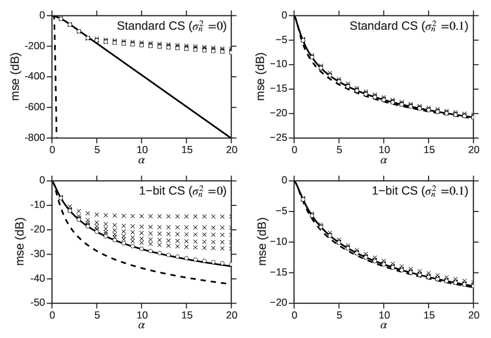
For noiseless standard CS, the offline reconstruction achieves $\mathsf{mse}=0$ when $\alpha$ is greater than a certain critical ratio $0<\alpha_{\rm c}(\rho)<1$ [13]. On the other hand, the analysis based on (7) indicated that $\mathsf{mse}\simeq O\left(\exp(-\alpha/\rho)\right)$ holds for large $\alpha$, which means that perfect recovery is unfortunately impossible with (4). However, this result may still promote the use of the online algorithm for very sparse signals with $0<\rho\ll 1$ where $\exp(-\alpha/\rho)$ becomes negligible.

For noiseless 1-bit CS, the result of [17] meant that $\mathsf{mse}\simeq(Q_{0}/2)\left(\frac{\rho}{K\alpha}\right)^{2}$ was asymptotically achieved by the offline method, where $K=0.3603\ldots$. On the other hand, (7) yielded the asymptotic form $\mathsf{mse}\simeq 2Q_{0}\left(\frac{\rho}{K\alpha}\right)^{2}$ for $\alpha\gg 1$. This indicates that online recovery can save computation and memory costs considerably while sacrificing $\mathsf{mse}$ by only a factor $4$ asymptotically.

These results may imply that there are fundamental gaps in the asymptotically achievable performance limit depending on the allowable computational costs in the absence of noise. However, this is not the case when Gaussian measurement noise is present, for which $P(y|u)$ becomes differentiable with respect to $u$. This property guarantees that $\hat{q}\simeq I\alpha$ asymptotically holds for both the online and offline methods, which yields a universal expression for the asymptotic MSE: $\mathsf{mse}\simeq 2\rho/\hat{q}=2\rho/(I\alpha)$, where

represents the Fisher information of the measurement model $P(y|u)$ averaged over the generation of $\bm{\Phi}^{t}$. This impresses the potential utility of the online algorithm and indicates that a performance similar to that of the offline method can be asymptotically achieved with a significant reduction in computational costs.

We developed an online algorithm to perform Bayesian inference on the signal recovery problem of CS. The algorithm can be carried out with $O(N)$ computational and memory costs per update, which are considerably less than those of the offline algorithm. From the algorithm, we also derived ordinary differential equations with respect to macroscopic variables that were utilized for the performance analysis. Our analysis indicated that the online algorithm can asymptotically achieve the same MSE as the offline algorithm with a significant reduction of computational costs in the presence of Gaussian measurement noise, while there may exist certain fundamental gaps in the achievable performance depending on usable computational resources in the absence of noise. Numerical experiments based on the standard and 1-bit scenarios supported our analysis.

Here, we assumed that correct knowledge about the prior distribution of signals and the measurement model is provided in order to evaluate the potential ability of the online algorithm. However, such information is not necessarily available in practical situations. Incorporating the idea of online inference into situations lacking correct prior knowledge is an important and challenging future task.

PVR acknowledges FAPESP for supporting his stay at the Tokyo Institute of Technology under Grant No. 2014/22258-2. This work was partially supported by JSPS KAKENHI No. 25120013 (YK).

References

- [1] T. Hey and A. E. Trefethen, Science 308, 817 (2005).
- [2] T. Hey, S. Tansley, and K. Tolle, eds., The Fourth Padadigm: Data-Intensive Scientific Discovery (Microsoft Research, 2009).
- [3] I. J. Taylor, E. Deelman, D. B. Gannon, and M. Shields, Workflows for e-Science: Scientific Workflows for Grids (Springer Publishing Company, Incorporated, 2014).
- [4] D. L. Donoho, IEEE Trans. Inform. Theory 52, 1289 (2006a).
- [5] E. J. Candès and M. B. Wakin, IEEE Signal Processing Magazine 25, 21 (2008).
- [6] D. L. Donoho, Discrete Comput. Geom. 35, 617 (2006b).
- [7] D. L. Donoho and J. Tanner, J. Am. Math. Soc. 22, 1 (2009).
- [8] E. J. Candès and T. Tao, IEEE Trans. Inform. Theory 51, 4203 (2005).
- [9] E. J. Candès and T. Tao, IEEE Trans. Inform. Theory 52, 5406 (2006).
- [10] Y. Kabashima, T. Wadayama, and T. Tanaka, J. Stat. Mech. Theor. Exp., L09003 (2009).
- [11] D. L. Donoho, A. Maleki, and A. Montanari, PNAS 106, 18914 (2009).
- [12] S. Ganguli and H. Sompolinsky, Phys. Rev. Lett. 104, 188701 (2010).
- [13] F. Krzakala, M. Mézard, F. Sausset, Y. F. Sun, and L. Zdeborová, Phys. Rev. X 2, 021005 (2012).
- [14] S. Rangan, A. K. Fletcher, and V. K. Goyal, IEEE Trans. Inform. Theory 58, 1903 (2012).
- [15] P. T. Boufounos and R. G. Baraniuk, in Proc. Conf. Inform. Science and Systems (CISS) (Princeton, NJ, 2008).
- [16] Y. Xu and Y. Kabashima, J. Stat. Mech. Theor. Exp., P02041 (2013).
- [17] Y. Xu, Y. Kabashima, and L. Zdeborová, J. Stat. Mech. Theor. Exp., P11015 (2014).
- [18] M. F. Duarte, S. Sarvotham, D. Baron, M. B. Wakin, and R. G. Baraniuk, in In Asilomar Conf. Signals, Sys., Comput (2005) pp. 1537–1541.
- [19] D. Baron, D. M. F., M. B. Wakin, S. Sarvotham, and R. G. Baranuik, pre-print (2009), http://arxiv.org/abs/0901.3403 .
- [20] Y. Shiraki and Y. Kabashima, J. Stat. Mech. Theor. Exp. , P05029 (2015).
- [21] O. Kinouchi and N. Caticha, J. Phys. A: Math. Gen. 25, 6243 (1992).
- [22] M. Biehl and P. Riegler, Europhys. Lett. 28, 525 (1994).
- [23] Y. Kabashima, J. Phys. A: Math. Gen. 27, 1917 (1994).
- [24] D. Saad and S. A. Solla, Phys. Rev. Lett. 74, 4337 (1995).
- [25] M. Opper, Phys. Rev. Lett. 77, 4671 (1996).
- [26] C. Van den Broeck and P. Reimann, Phys. Rev. Lett. 76, 2188 (1996).
- [27] R. Vicente, O. Kinouchi, and N. Caticha, Machine Learning 32, 179 (1998).
- [28] D. Saad, ed., On-Line Learning in Neural Networks (Cambridge University Press, 1998).
- [29] S.-i. Amari and H. Nagaoka, Methods of Information Geometry (American Mathematical Soc., 2007).
- [30] M. Opper and O. Winther, “On-line learning in neural networks,” (Cambridge University Press, 1998) Chap. A Bayesian approach to on-line learning, pp. 363–378.
- [31] O. Winther and S. A. Solla, “On-line learning in neural networks,” (Cambridge University Press, 1998) Chap. Optimal perceptron learning: as online Bayesian approach, pp. 379 – 398.
- [32] S. Rangan, pre-print (2010), arXiv:1010.5141 [cs.IT] .