Electron Thermodynamics in GRMHD Simulations of Low-Luminosity Black Hole Accretion
Abstract
Simple assumptions made regarding electron thermodynamics often limit the extent to which general relativistic magnetohydrodynamic (GRMHD) simulations can be applied to observations of low-luminosity accreting black holes. We present, implement, and test a model that self-consistently evolves an entropy equation for the electrons and takes into account the effects of spatially varying electron heating and relativistic anisotropic thermal conduction along magnetic field lines. We neglect the back-reaction of electron pressure on the dynamics of the accretion flow. Our model is appropriate for systems accreting at of the Eddington accretion rate, so radiative cooling by electrons can be neglected. It can be extended to higher accretion rates in the future by including electron cooling and proton-electron Coulomb collisions. We present a suite of tests showing that our method recovers the correct solution for electron heating under a range of circumstances, including strong shocks and driven turbulence. Our initial applications to axisymmetric simulations of accreting black holes show that (1) physically-motivated electron heating rates that depend on the local magnetic field strength yield electron temperature distributions significantly different from the constant electron to proton temperature ratios assumed in previous work, with higher electron temperatures concentrated in the coronal region between the disc and the jet; (2) electron thermal conduction significantly modifies the electron temperature in the inner regions of black hole accretion flows if the effective electron mean free path is larger than the local scale-height of the disc (at least for the initial conditions and magnetic field configurations we study). The methods developed in this work are important for producing more realistic predictions for the emission from accreting black holes such as Sagittarius A* and M87; these applications will be explored in future work.
Keywords:
MHD — general relativity — black hole accretion1 Introduction
A wide variety of low luminosity accreting black holes are currently interpreted in the context of a Radiatively Inefficient Accretion Flow (RIAF) model that describes a geometrically thick, optically thin disc with a low accretion rate and luminosity. In particular, this is true of the black hole at the center of our galaxy, Sagittarius A* (Narayan et al., 1998), the black hole at the center of Messier 87 (Reynolds et al., 1996), and other low luminosity Active Galactic Nuclei (AGN), as well as a number of X-ray binary systems (see Remillard & McClintock 2006 for a review). The gas densities in these systems are low enough that the time scale for electron-ion collisions is much longer than the time scale for accretion to occur, so a one-temperature model of the gas is no longer valid (as originally recognised by Shapiro, Lightman & Eardley 1976, Ichimaru 1977, and Rees, Begelman, Blandford, & Phinney 1982). Instead, a better approximation is to treat the electrons and ions as two different fluids, each with its own temperature.
Calculating the emission from accreting plasma requires predicting the electron distribution function close to the black hole. To date, time dependent numerical models of RIAFs that attempt to directly connect to observations often assume a Maxwellian distribution with a constant electron to proton temperature ratio, , and take the results of GRMHD simulations as the solution for the total gas temperature, (Dibi et al., 2012; Drappeau et al., 2013; Mościbrodzka et al., 2009). This neglects, however, several physical processes that have different effects on the electron and proton thermodynamics and that are currently only included in one-dimensional semi-analytic models. Such effects include electron thermal conduction (e.g., Johnson & Quataert 2007), electron cooling (e.g., Narayan & Yi 1995), and non-thermal particle acceleration and emission (e.g., Yuan, Quataert & Narayan 2003). To date, extensions of the simple const. prescription have been limited to post-processing models that do not self-consistently evolve the electron thermodynamics over time. Examples include the prescription of Mościbrodzka et al. (2014) which takes const. in the disc proper but sets const. in the jet outflow region, as well as the model of Shcherbakov, Penna & McKinney (2012), who solve a 1-D radial equation for at a single time-slice in the midplane to obtain a functional relationship that is then applied to the rest of the simulation. To enable a more robust connection between observations of accreting black holes and numerical models of black hole accretion, it is critical to extend the detailed thermodynamic treatment of electrons used in 1D calculations to multi-dimensional models. This is the goal of the current paper. In particular, we describe numerical methods for separately evolving an electron energy equation in GRMHD simulations. We focus on including heating and anisotropic thermal conduction in these models. Future work will include electron radiative cooling and Coulomb collisions between electrons and protons.
In a turbulent, magnetised plasma, electrons and ions are heated at different rates depending on the local plasma conditions (e.g., Quataert & Gruzinov 1999; Cranmer et al. 2009; Howes 2010; Sironi 2015). Furthermore, since the electron-to-proton mass ratio is small, electrons will both conduct and radiate their heat much more efficiently than the ions. The combination of these effects leads to the expectation that, in general, . In the present paper, we thus neglect the effect of the electron thermodynamics on the overall dynamics of the accretion flow. This allows us to treat the simulation results as a fixed background solution on top of which we independently evolve the electrons. Even if we find that in some regions of the disc, this treatment may still be a reasonable first approximation given the uncertainties in the electron physics.
The neglect of electron cooling in the present paper is reasonable for systems accreting at of the Eddington rate, , so that the synchrotron cooling time is much longer than the accretion time (Mahadevan & Quataert, 1997). In particular, this likely includes Sagittarius A* in the galactic center. The application of our methodology to Sgr A* is particularly important given the wealth of multi-wavelength data (e.g., Serabyn et al. 1997, Zhao et al. 2003, Genzel et al. 2003, Baganoff et al. 2003, Barrière et al. 2014) and current and forthcoming spatially resolved observations with the Event Horizon Telescope (Doeleman et al., 2008) and Gravity (Gillessen et al., 2010).
The goal of this paper is to present our formalism and methodology for evolving the electron thermodynamics and to apply the results to 2D (axisymmetric) GRMHD simulations of an accreting black hole. We show the range of possible electron temperature distributions in the inner region of the disc, which directly impacts the predicted emission. Future work will explore the impact that these results have on the emission, spectra, and images of Sagittarius A*.
The remainder of this paper is organised as follows. §2 describes our theoretical model of electron heating and anisotropic electron conduction while §3 describes the numerical implementation of this model. §4 contains tests of the numerical implementation, §5 applies the model to a 2D simulation of an accretion disc around a rotating black hole, and §6 discusses the implications of this application and concludes. Boltzmann’s constant, , and proton mass, , are taken to be 1 throughout. We use cgs units, with Lorentz-Heaviside units for the magnetic field (e.g., magnetic pressure is ), and a metric signature of . We also assume that the gas is mostly hydrogen and ideal. Since we also assume , then (setting ), so we use and interchangeably.
2 Electron Thermodynamics
The accreting plasmas of interest are sufficiently low density that the electron-proton Coulomb collision time is much longer than the dynamical time and so a two-temperature structure can develop, with the protons and electrons having different temperatures (and, indeed, different distribution functions). Moreover, at the low accretion rates where radiative cooling can be neglected, the electron-electron and proton-proton Coulomb collision times are also much longer than the dynamical time (Mahadevan & Quataert, 1997). However, the plasma densities are high enough that the plasma is nearly charge-neutral and so we assume that . We further assume that the electron flow velocity is the same as that of the protons.11 1 More precisely, as in standard MHD, the relative velocity between electrons and protons required to produce currents that can maintain magnetic fields near is orders of magnitude less than the mean sound speed. This need not strictly be true (e.g., in the solar wind the relative velocities of particle species can be of order the Alfven speed; e.g. Bourouaine et al. 2013 ), but is a reasonable first approximation. A similar approach is often used in modeling the global dynamics of the low-collisionality solar wind (e.g., Chandran et al. 2011).
Under these assumptions, the key difference in the electron and proton physics lies in their different thermodynamics: the protons and electrons have very different heating and cooling processes that need to be separately accounted for. Formally, because of the low collisionality conditions we should separately solve the electron and proton Vlasov equations. This is computationally extremely challenging, however, particularly in the global geometry required to predict the emission from accreting plasmas (even local shearing box calculations using the particle-in-cell technique to solve the Vlasov equation require an unphysical electron-proton mass ratio, thus making it difficult to reliably model the electron thermodynamics; e.g., Riquelme et al. 2012). As a result, we assume a fluid model in this paper. Our fluid approximation corresponds to taking moments of the Vlasov equation and applying closures on higher moments of the distribution function. As we shall describe, our closure corresponds to specific models for the conductive heat flux, the viscous momentum flux, and the turbulent heating rate of each particle species.
Our basic model is thus to take a single-fluid GRMHD solution (e.g., Komissarov 1999; Gammie, McKinney & Tóth 2003; De Villiers & Hawley 2003) as an accurate description of the total fluid (composed of both the electron and proton gas) dynamics and thus the accretion flow density, magnetic field strength, and velocity field. We evolve the electrons as a second fluid on top of this background solution. The GRMHD solution may itself include viscosity and conduction as in Chandra et al. (2015). Our assumption that the electrons do not back react on the flow dynamics is formally valid in the limit that , but should be a reasonable approximation so long as in regions of large plasma , i.e., where gas pressure forces are dynamically important. One advantage of not coupling the electron pressure to the GRMHD solution is that we can run multiple electron models in one simulation, allowing us to explore systematic uncertainties with a minimum of computational time.
In this paper, we focus on implementing electron heating and anisotropic conduction. Coulomb collisions are straightforward to include but are negligible for the low accretion rates at which electron cooling can be neglected. In future work, electron cooling will be self-consistently incorporated building on the BHlight code developed by Ryan, Dolence & Gammie (2015).
2.1 Basic Model
The stress-energy tensors for the electron and proton fluids in our model take the form:
| (1) | ||||
where , , and are the fluid frame density, internal energy, and pressure, respectively, is the fluid four-velocity in the coordinate frame, is a general stress tensor that accounts for viscous effects, and is the heat flux carried by the electrons. The subscript denotes or (and will also denote the total gas quantities labeled by below). We leave as a general tensor that will be model-specific. For each species, ignoring electron-electron, electron-ion, and ion-ion collisions, one can take the zeroth and first moment of the Vlasov equation to show that
| (2) |
and
| (3) | |||
where is the electromagnetic field tensor. In ideal, single-fluid GRMHD in the absence of shocks, the conservation of entropy equation, , where is the entropy per particle, follows directly from the conservation of particle number and the stress-energy (see page 563 in Misner, Thorne & Wheeler 1973). To derive entropy equations for the electron and proton fluid used in our model, we perform the same series of manipulations; namely, contracting both equations (3) with (the total fluid velocity, which we take to be ) and invoking equation (2), which give us:
| (4) |
and
| (5) |
where we have defined the heating rate per unit volume for each species as a sum of viscous and Ohmic resistance terms, and , and where is the four-acceleration, which accounts for gravitational redshifting of the temperature by the metric. We can write the heating rates in terms of the electric field four-vector, , and the four-currents, , as22 2 We have kept the subscripts and for the four-currents (and thus four-velocities) in equation (6) because the details of the Ohmic heating depend on the small but non-zero velocity difference between the proton and electron fluids (or equivalently the velocity difference between the electron/proton fluid and the total fluid). An explicit expression for these terms would require a detailed kinetic theory calculation beyond the scope of the present work (i.e., some form of “generalized Ohm’s Law,” as in, e.g., Koide 2010). In our model, as described in the text, numerical resistivity provides the Ohmic heating that is then distributed to electrons and protons according to a closure model obtained from previous work in kinetic theory. :
| (6) | ||||
The intuitive understanding of the Ohmic heating terms on the right-hand side of equation (6) is that they are evaluated in the rest frame of the total fluid. To derive the entropy equation for the total fluid, we first define several total fluid variables as a sum of electron and proton terms: , , , , and , denoting total gas mass density, internal energy, pressure, temperature, current, and viscous stress. Then, using the thermodynamic identity, , we find that the entropy per particle of the total gas, , satisfies the relation , resulting in
| (7) |
with the total heating rate per unit volume:
| (8) |
In practice, we use the electron entropy equation (5) to evolve the electron thermodynamics. To determine the overall dynamics of the electron + proton gas, we use Maxwell’s equations in addition to a standard, single-fluid GRMHD evolution representing the total gas. The equations for the latter are obtained by separately summing the electron and proton parts of equation (2) and equation (3), resulting in a mass conservation equation,
| (9) |
and an energy-momentum equation,
| (10) |
with the total gas stress-energy tensor,
| (11) |
and the electromagnetic stress energy tensor33 3 Here we have chosen to absorb a factor of into the definition of ., . We have used the identity in equation (10), the assumption that in equation (11), and the charge-neutrality assumption throughout. Furthermore, we have dropped the electron thermal conduction terms in the evolution of the total gas properties, though we keep them in the evolution of the electron entropy (equation 5). This is consistent if since electron conduction will then affect the electron thermodynamics but not the overall stress-energy of the fluid. Finally, we take to be given by the ideal MHD limit (i.e., ):
| (12) |
where is the magnetic field four-vector defined in terms of the Levi-Civita tensor, , and is twice the magnetic pressure. With these assumptions, equations (9), (10), and Maxwell’s equations are simply the standard single-fluid equations of ideal GRMHD except with an explicit viscosity tensor. In standard conservative GRMHD codes (including the one used in this work), this viscosity tensor is not included explicitly but implicitly generated numerically by the Riemann solver. Furthermore, the Riemann solver also introduces a finite numerical resistivity into Maxwell’s equations, allowing for a nonzero (and thus nonzero Ohmic heating). For further discussion of these points, see § 3.1.
To summarise, we take a standard single fluid GRMHD evolution of , and as a reasonable estimate of the total gas properties. This corresponds to assuming that electron conduction has a negligible contribution to the dynamics of the total gas and that the adiabatic index is independent of the electron thermodynamic quantities (e.g.; some function of total gas quantities only). Formally, this assumption requires that the electron internal energy is small compared to the proton internal energy. From this, we can calculate the heating directly from equation (7) (dropping the conduction terms) without requiring an analytic expression for . Finally, we use knowledge of the nature of heating in a collisionless plasma obtained from kinetic theory (described in §5.1) to relate the heating rate per unit volume of the electrons, , to that of the total fluid, , and directly add it to the electron entropy equation (equation 5), as described in §2.2. This completes our model.
For simplicity, we assume that the adiabatic indices of the electron, , proton, , and total gas, , are constants, where for or . This simplifies the numerical implementation of the model, as it allows us to write the entropy per particle in a simple form, , and avoids the complication of having to evaluate when updating the total fluid variables. This can be seen by noting that
| (13) |
which is only constant in the limits that or . From this, we see that this simplification of const. is formally inconsistent if , which is generally the case in the accreting systems of interest, where the electrons are typically relativistically hot () but the protons are nonrelativistic (. However, since equation (13) is bounded between and and we expect , we do not anticipate that this approximation will affect our results significantly.
2.2 Electron Heating
We parameterise the heating term, in equation (6) by writing = , where is the fraction of the total dissipation, , received by the electrons. This function, in general, depends on the local plasma environment and our model is not limited to any particular choice of . As knowledge in the field develops we can readily incorporate different assumptions about electron heating. A more detailed discussion of one physically-motivated prescription for is given in §5.1. Given a GRMHD solution, the total heating rate of a fluid element moving with four-velocity in the coordinate frame can be computed (from equation 7, dropping the conduction terms):
| (14) |
where is the entropy per particle. We can rewrite equation (14) in terms of , where , as . We use to avoid the undesirable numerical properties of logarithms as the argument goes to 0. Likewise, we will often use in place of in equation (5).
2.3 Anisotropic Electron Conduction
Some care must be taken when generalising the theory of anisotropic conduction along magnetic field lines to a relativistic and covariant formulation. In particular, the theory must be consistent with causality in that the heat flux should not respond instantly to temperature gradients. Our formulation of anisotropic electron conduction draws heavily on the treatment of Chandra et al. (2015), who consider a single fluid model in which the heat flux is coupled to the dynamics via the stress-energy tensor. We give a brief summary of our approach here, highlighting those aspects of our electron-only treatment that differ from the formulation in Chandra et al. (2015).
One can derive a perturbation solution for the heat flux, , by expanding the entropy current in powers of and imposing the second law of thermodynamics. The most straightforward relativistic generalisation of the classical, isotropic heat flux first written down by Eckart (1940) is first order in this expansion and was later shown by Hiscock & Lindblom (1985) to be unconditionally unstable, precisely because it violated causality (Chandra et al. 2015 showed the same for anisotropic conduction). Israel & Stewart (1979) derived a second order solution for which was later shown to be conditionally stable (Hiscock & Lindblom 1985; Chandra et al. 2015). Here we use a first order reduction of that second order model that has been shown to be both stable and self-consistent (Andersson & Lopez-Monsalvo, 2011). We refer the reader to Chandra et al. (2015) for more details.
We parameterise the heat flux as
| (15) |
where is a unit vector () along the magnetic field four-vector, , and the scalar is given by the following evolution equation:
| (16) |
where is the determinant of the metric, and we used an identity, , to convert covariant derivatives into partial ones (Landau & Lifshitz, 1975, eq. 86.9 in). Here is the equilibrium value of the heat flux given by
| (17) |
where is the thermal diffusion coefficient of the electrons and is the relaxation time scale for the heat flux over which it responds to temperature gradients. Note that equation (16) is a relaxation equation in which the heat flux relaxes on a timescale to the equilibrium value.
The equilibrium heat flux in equation (17) is the natural relativistic extension of anisotropic conduction along the magnetic field (analogous to the isotropic heat flux of Eckart 1940). The heat flux, , then contributes to the electron energy equation as in equation (5). Physically motivated prescriptions for the parameters and are all that are required to complete the model. We discuss one choice of these in §5.1.
2.3.1 Stability of Anisotropic Electron Conduction Theory
In our formalism, we assume that the fluid velocity, , and the electron number density, , are independent of the electron thermodynamics. Thus, in order to do a perturbative analysis we need only perturb the electron temperature, , and the heat flux, , in equations (5) and (16). Doing this in the fluid rest frame in Minkowski space, where , and writing the perturbations in Fourier space as , we find the dispersion relation:
| (18) |
with the solutions:
| (19) |
The theory is unstable if , which can only occur if the term under the square root is both real and greater than unity. However, this is impossible for any value of when , so we conclude that equations (5) and (16) are unconditionally stable. This is in contrast to the case where equations (5) and (16) are coupled to the ideal MHD equations, which is unstable to small perturbations unless the relaxation time is larger than a critical value (Hiscock & Lindblom 1985; Chandra et al. 2015).
3 Numerical Implementation of Electron Heating and Conduction
The method outlined above can, in general, be applied to any GRMHD “background” simulation. For the rest of this work, however, we will consider only conservative codes, as the equations of ideal MHD can be naturally written in that form. Because of this, in what follows we will seek to put all of our evolution equations in a conservative form, namely:
| (20) |
where is a “conserved” variable, is the corresponding flux in the th direction, and is the source, which in general includes the contribution from the connection coefficients. Equation (20) can then be approximated in one spatial dimension by the following discretisation:
| (21) | ||||
where the fluxes are evaluated at face centres using the chosen Riemann solver. The generalisation to higher dimensions is straightforward.
With that in mind, we can rewrite equation (5):
| (22) |
where we have used the definition . Note that equation (22) is a quasi-conservative equation with and (‘quasi’ conservative because the standard definition of conservative equations excludes source terms with derivatives). To solve equation (22), we use operator splitting in the following sequence of steps:
- 1.
Solve the conservative equation with .
- 2.
Explicitly update with the heating term (the first term in the brackets in eq. 22).
- 3.
Implicitly solve a matrix equation to include the conduction source terms (the rest of the terms in square brackets in eq. 22).
Steps 2 and 3 are described in detail in §3.3 and §3.4, respectively, while step 1 will be specific to the choice of the background numerical scheme.
3.1 Heating in Conservative Codes
Formally, the equations of ideal MHD used by conservative GRMHD simulations imply that the heating rate per unit volume, , in equation (8) is identically zero. However, conservative codes implicitly add numerical viscosity and resistivity terms to the stress-energy tensor and Maxwell’s equations, respectively. The former implies that the numerically evolved stress tensor is in fact for some numerical viscosity tensor , while the latter implies . The numerical resistivity can be thought of as implicitly introducing a form of Ohm’s law that allows for a nonzero electric field four-vector, . Thus, even though the energy implied by is conserved to machine precision (see below for details), experiences truncation-level heating. This manifests itself as entropy generation: truncation errors lead to dissipation of magnetic and kinetic energy close to the grid scale that is captured as internal energy. We use this change in entropy to directly calculate the heating rate per unit volume of the gas, .
Although is conserved to machine precision, the second law of thermodynamics is satisfied only to truncation error. Thus there can be locally regions with . In particular, the truncation error can be positive or negative, so in places with small actual change in entropy or large truncation error the change in entropy can be negative. This is the case even in test problems in which our methods of calculating the heating give the correct, converged, answer for the fluid variables (see § 4). Thus, while may be instantaneously or locally negative, when integrated over a sufficient length of time and/or space in the fluid frame it will satisfy the second law of thermodynamics.
We choose this method of calculating the heating rate as opposed to introducing an explicit functional form for because it seems reasonable to assume that for several applications, the grid-scale dissipation in conservative codes is a well-defined quantity determined by the converged large-scale physics of the problem. Turbulence, for example, takes kinetic and/or magnetic energy at the largest scales and cascades it down to a small dissipative scale where it is converted into internal energy. For a numerical scheme with no explicit viscosity, the scale at which dissipation occurs depends entirely on the resolution of the simulation, but we expect the heating rate itself will be fixed (in an averaged sense; see, e.g., Davis, Stone & Pessah 2010). We expect the same for forced reconnection at high values, as in the disc midplane, where the large-scale dynamics sets the rate at which the field lines of opposite sign are brought together.
The above argument relies on the conservation of energy. In an arbitrary space-time, however, conservation of energy is only well-defined if the metric is stationary (time-independent) and therefore possesses a time-like Killing vector, . If such a vector exists (as it does for the Kerr metric of interest in this work), we can construct a conserved current from the stress-energy tensor via , where this current satisfies . This allows us to define a conserved energy in a coordinate basis:
| (23) |
where the integral is over all space (i.e. the space orthogonal to the time coordinate). Often, the Killing vector takes the form , which simplifies equation (23) to
| (24) |
Thus, can be thought of as the conserved energy per unit volume for a particular choice of coordinates. The total energy, , is conserved to machine precision, modulo fluxes of energy through the boundaries, so entropy can only be generated by conversion of one form of energy to another.
3.2 Calculating the Total Heating Rate
To calculate the heating generated at each time step, we introduce an entropy-conserving equation as a reference to compare with the energy conservation equation. The entropy-conserving equation is simply a conservation equation like equation (20) with , , and . If we call the solution to this equation (the denotes the solution corresponding to entropy conservation), then we show in Appendix B.1 that the total heating rate of the fluid (measured in the fluid rest frame) incurred over an interval (measured in the coordinate frame),
| (25) |
where accounts for the transformation of from the coordinate frame to the fluid rest frame, and denote the values at the beginning and the end of the time step, respectively, so that , and denotes the values when calculating the fluxes. To compute the dissipation rate via eq. (25), we set at the beginning of each time step and use when calculating the fluxes. Physically, equation (25) means that the Lagrangian heating rate is set by the difference between the entropy implied by the total energy conserving solution () and the entropy implied by the entropy conserving solution ().
3.3 Electron Heating Update
Let us call the solution to equation (22) without any source terms. On top of this adiabatic evolution, electrons receive a fraction, , of the heating of the gas, . In discrete form, this can be written as follows,
| (26) |
Therefore, the heating update to the electrons, , takes the following form:
| (27) |
3.4 Electron Conduction Update
We note that the evolution equation for the heat flux (equation 16) is already in a quasi-conservative form if we define and . We treat the evolution of in an operator split way similar to the evolution of with the following series of steps:
- 1
Solve the conservative equation with .
- 2
Implicitly solve a matrix equation to include the source terms.
The source terms in the electron entropy and equation due to conduction are given by:
| (28) | ||||
which are discretised in space by using slope-limited derivatives across three grid cells and discretised in time by centring the time derivatives at . The latter discretisation gives us an implicit equation for the variables and at time . If we call the heat flux after being updated by step 1, and the electron entropy after being updated by heating, then this matrix equation takes the form:
| (29) |
with components
| (30) | ||||
and
| (31) | ||||
The system of equations has a straightforward solution,
| (32) |
To ensure that the heat flux, , does not reach unphysically large values, we apply a limiting scheme to keep , where and is the electron thermal speed. Since we are considering physical systems in which the electrons are always at least mildly relativistic, this limit effectively reduces to , which corresponds to a ‘saturated’ heat flux in which the heat is redistributed at the electron thermal speed. The numerical implementation of this limit is to replace the values of the thermal diffusivity, , and the relaxation time-scale, , with ‘effective’ values (Chandra et al., 2015):
| (33) |
and
| (34) |
where
| (35) |
which sharply transitions from for some small as . Thus, according to equation (16), when , decays exponentially on a timescale until it drops below . The parameter is chosen such that the criterion for numerical stability is always satisfied (see §3.4.1 and Appendix B.3).
3.4.1 Numerical Stability of Electron Conduction
A detailed derivation of the criteria for numerical stability is in Appendix B.3. The basic result is that for a Courant-Friedrichs-Lewy (CFL) number, , reasonably chosen between and , the relaxation time, , must satisfy
| (36) |
where is a function of the CFL number. This can be understood as a requirement that the relaxation time (which we are free to choose as arbitrarily large, though which should correspond to a physical time scale), must be larger than the time step (which is limited by computational expense) by the ratio between and the standard Courant limit for a diffusive process .
3.5 Treatment of the Floors
Conservative codes deal poorly with vacua of internal energy and density. Because of this, many schemes employ floors on internal energy and density to ensure that the errors in solving for the primitive variables from the conservative variables do not produce unphysically small or negative values. The nature of the model outlined above requires special care to be taken when these floors are activated, as they introduce artificial changes in internal energy, which act as a source of heat, and density, which change the conversion between entropy and internal energy.
3.5.1 Electron Energy Floors
Though the second law of thermodynamics states that the heating term should be positive definite, numerically we find that can be locally negative because of truncation errors. This introduces the possibility of the electron internal energy going to zero (or even becoming negative) due to truncation error fluctuations in our heating term. To correct for this, we implement a floor on the electron internal energy that is of the floor on the total gas internal energy. That is, if drops below , we reset to .
3.5.2 Total Gas Internal Energy Floors
When the floor on internal energy of the total gas is activated, there is an artificial increase in which then shows up in our heating term. We treat this addition of energy as if it were a physical, isochoric addition to the energy of the gas and add it to the electrons as described above. We emphasise that the internal energy floor does not affect the system dynamics in any significant way because it is only activated in magnetically-dominated regions where the value of the internal energy is dynamically irrelevant.
3.5.3 Density Floors
When the floor on density is activated, the total gas internal energy remains unchanged. However, the value of increases by a factor of , where is the pre-floor density. To correct for this, we require conservation of the evolved gas entropy when the density floor is activated by decreasing by a factor of . Furthermore, we enforce that the evolved electron entropy remains unchanged by the density floor in the same manner by decreasing by a factor of . Similar to the internal energy floors, the density floors do not affect the dynamics of the system.
4 Tests of Numerical implementation
In this section we describe a series of tests that demonstrate the robustness and accuracy of our method of evolving the electron internal energy. We implemented the model described in §2 and §3 into the conservative GRMHD code, HARM2D (High-Accuracy Relativistic Magnetohydrodynamics; Gammie, McKinney & Tóth 2003; Noble et al. 2006). To speed up the computations, we parallelised the code using OpenMP and MPI via domain decomposition.
4.1 Tests of Electron Heating
In what follows we demonstrate the validity and convergence of our implementation of electron heating using a number of tests. The 2nd order convergence of HARM in smooth flows and 1st order convergence in discontinuous flows is well documented in Gammie, McKinney & Tóth (2003) and we will not reproduce it here.
4.1.1 Explicit Heating in a Hubble-Type Flow
To test whether our discretizations of the heating is correctly time centred, i.e., converges at the expected 2nd order in time, we focus here on solving the electron equation when we introduce an explicit heating term to the total energy equation. We do this in an unmagnetised, 1D Hubble-type flow with (restricting ourselves to non-relativistic velocities). In the local rest frame of a fluid element, this velocity field gives an outflow in both directions that is homogenous and isotropic, causing the density to uniformly decrease with time as matter leaves the computational domain. The velocity profile also scales with time to satisfy the momentum equation . In the absence of heating, the internal energy and pressure evolve according to entropy conservation (), so that the solution at later times is given by (Tchekhovskoy, McKinney & Narayan, 2007):
| (37) | ||||
If we now add a cooling term to the energy equation, of the form:
| (38) |
the internal energy should evolve as
| (39) |
Plugging these solutions in the electron entropy equation (22) for and , we obtain:
| (40) |
For the numerical test, we set these analytic solutions as the boundary and initial conditions in a one-dimensional grid and check if we maintain this solution after a dynamical time of . We set , , , and , on a computational domain of . Formally, since , the choice of is unphysical. However the motivation for this choice stems from the fact that our primary application is to the inner regions of an accretion disc around a black hole, where we expect . We find that our calculation converges at second order (see Figure 1), up until the point at which the errors in the analytic solution due to relativistic effects become important (which, for is ).

4.1.2 1D (Noh) Shock Test
In Appendix B.4, we show that for a high Mach number shock in which the electrons are assumed to receive a constant fraction of the ‘viscous’ heating in the shock, the post shock electron internal energy is given by:
| (41) |
where and are the post-shock internal energy and the adiabatic index of the fluid. Equation (41) assumes that the electrons do not back react on the shock structure, consistent with the model developed in this paper. When , equation (41) is equal to , while for and it is . Here we check whether our numerical implementation of electron heating is consistent with this result.
The initial conditions for this test are an unmagnetised, non-relativistic (), uniform density and internal energy fluid. The velocity profile is discontinuous at the center of the grid, with a left and a right state given by . The resulting solution is two shocks propagating outwards with a static region in between. We focus on a non-relativistic ( flow of initially cold gas so that the Mach number of the flow satisfies . For this test we fix and show the results for both and .
Figure 2 shows the density and electron internal energy as a function of position for a shock with at , where is the size of the computational domain. Figure 3 shows that our simulation converges at 1st order to the analytic result for the post-shock electron internal energy when but to a value differing from the expected result by when (Figure 2). This difference is smaller at lower Mach number, as shown explicitly in Figure 4. The modest discrepancy between the analytic post-shock electron temperature and the HARM solution is because an accurate, converged calculation of the heating term requires a well-resolved shock structure that gets better resolved at higher resolution. This is not the case for modern shock capturing techniques, for which the numerical width of the shock is always a few grid points and our heating calculation is never able to resolve the shock. This is not an issue when because the factors of density in equation (27) cancel, removing the dependence on the shock structure. We show in Appendix C that introducing an explicit bulk viscosity leads to convergence to the analytical result at 2nd order for . However, the error as seen in Figures 2 and 4 is sufficient for our purposes so we do not include a bulk viscosity in our calculations.


4.1.3 2D Forced MHD Turbulence Test
Another test problem with a known, converged heating rate is driven turbulence in a periodic box. If we inject the fluid with a constant energy input rate of at large-scales, we should find that after saturation of kinetic and magnetic energies has been reached. Thus, for the electron heating model outlined above, after this saturation point the electrons should receive a fraction of . Furthermore, if we have a periodic box in which the particle number is fixed, then the total internal energy change from adiabatic expansion/compression will sum to zero. Thus the analytic result we expect for our model of electron heating is that . This test checks whether our model satisfies this result numerically.
We start with a static, uniform density fluid with and sound speed in a 2D periodic box. The initial magnetic field is uniform: the magnetic field lines are straight and lie in the plane of the simulation. Then, at each time step, we give Gaussian random kicks to the velocity such that the wave number satisfies (i.e. the driving is incompressible), and (compare to Lemaster & Stone 2009). The normalisation is fixed such that the rate of energy injection is equal to . This leads to a rms turbulent velocity that is , so that the turbulence is subsonic and roughly Alfvénic. The peak driving wave number is set to half the box size: . Furthermore, we ensure that no net momentum is added to the box by subtracting off (from the kicks) any average velocity that would have been generated by the kicks. For this test we fix , and .
Figure 5 shows our results for the electron and total internal energies as a function of time in the box at . We see that once approximate saturation of the turbulence is reached at (or in the figure), the internal energies are in very good agreement with a linear fit, as expected given the constant rate of energy injection. For a parameterization of and , and represent the electron and total heating rates, respectively. These can be compared to the energy injection rate, , which is a fixed constant of . At a resolution of , we find the total heating rate differs from by , while the electron heating rate differs from by . Unfortunately, a rigorous convergence study of these quantities is not possible because of the nature of turbulence in 2D. Due to the inverse energy cascade, the kinetic and magnetic energies never truly saturate and convergence of any of the fluid variables is never achieved. This can be seen from Table 1, where the values of and are quoted at various resolutions, neither of which display significant convergence to the expected and , respectively. Nevertheless, we find the percent level error found at all resolutions to be sufficiently small to satisfy our error tolerance in the full accretion disc simulation.

| Resolution: | 128 | 256 | 512 |
|---|---|---|---|
| 44 4 Fractional error in the electron heating rate relative to the analytic solution. | |||
| 55 5 Fractional error in the total heating rate relative to the analytic solution. |
4.1.4 Shadow Solution
For our two-temperature model, we can seek a solution in which the electron fluid simply ‘shadows’ the total gas, in that . Such a solution is found by setting at some initial time, since we can solve the first law of thermodynamics for the electrons with for all time, assuming that and is a constant. This can be seen from the first law:
| (42) |
because the electrons will always get a fraction, of the entropy-generated heat (the first term on the RHS of equation 42), while the compression term is directly proportional to . This solution is valid regardless of the details of the overall fluid evolution, so we can apply it to an arbitrarily complicated system.
For this test, we evolve the electron internal energy in the full accretion disc simulation around a rotating black hole as outlined in §5. We initially apply small () perturbations to the electron internal energy about the average value of , and set and . For this test alone, we set the floor on electron internal energy to be a fraction of the floor on the total fluid (as opposed to our usual choice of ). If this latter step were neglected, the floors would cause the polar regions to differ significantly from the expected result, though leaving the disc and corona unaffected (i.e. they still satisfy the analytic result). The test is whether or not our simulation can maintain this result over the run time of .
Running this test at a resolution of gives an average fractional error of
| (43) |
which is smaller than our initial perturbations and shows that our numerical solution correctly evolves equation (42) even in a complex problem with MHD turbulence, weak shocks, and other heating processes in the presence of a curved metric.
4.2 Tests of Electron Conduction
Our model and testing suite for conduction closely resembles that of Chandra, Foucart & Gammie (2015), so we leave the details to Appendix A. In summary, we have found second order convergence for linear modes, for a static, 1D atmosphere in the Schwarzschild metric, and for a relativistic, spherically symmetric Bondi accretion flow. We also show that the electrons properly conduct along field lines in a 2D test.
5 Application to an Accreting Black Hole in 2D GRMHD Simulations
We apply the new methods discussed in §2 and the numerical implementation described in §3 to the astrophysical environment of an accretion disc surrounding a spinning black hole as described by the Kerr Metric with a spin parameter of . For this spin the last stable circular orbit is and the thin disc radiative efficiency is (Novikov & Thorne, 1973). We use the conservative code HARM (Gammie, McKinney & Tóth, 2003) as our background GRMHD solution. Our initial conditions for the total fluid are the Fishbone & Moncrief (1976) equilibrium torus solution (see Appendix D) with inner radius and with the maximum density of the disc occurring at . Note that here and throughout and refer to the Boyer-Lindquist coordinates. This equilibrium solution has a temperature maximum of and a thickness66 6 Here we define . of at . We normalise the torus density distribution such that the maximum value of density in the torus is and perturb the internal energy of the gas with random kicks on the order of to provide the perturbations for the magnetorotational instability (MRI, Balbus & Hawley 1991) to develop.77 7 In addition to the electron specific floor described in §3.5.1, there are also floors on the density and internal energy of the HARM single fluid GRMHD solution. These are and . Note that the unit choice for the background ”atmosphere” is such that the initial torus maximum density is and the initial torus internal energy is . We overlay this equilibrium solution with an initial magnetic field with (where max refers to the maximum value inside the torus), defined by the scalar vector potential:
| (44) |
if and 0 otherwise. This vector potential defines two meridional loops contained in the torus that are antisymmetric about the equator. This choice ensures that the field lines are not along constant density. Since constant density implies constant temperature when entropy is constant, field lines along constant density would be isothermal in the initial condition (as would happen if we dropped the factor of in eq. 44). 2D MHD torus simulations are unable to reach a statistical steady state in which the initial conditions are forgotten, so initially isothermal field lines could artificially suppress electron conduction even at later times. We choose the 2-loop initial condition to avoid this.
For the electrons, we start with , and run two different models for , described below. For conduction runs, we set the initial heat flux to zero.
Our conduction runs are all in grids with a physical size of the domain in spherical polar coordinates of , where is the black hole event horizon radius. For , . In the regions with , the code uses modified Kerr-Schild coordinates (, , , and ) of Gammie, McKinney & Tóth (2003), so that the regions with the highest resolution are near the mid-plane close to the horizon. For , we use hyper-exponential coordinates to move out the outer radial boundary and limit unphysical reflection effects by defining the internal code coordinate implicitly by the equation (Tchekhovskoy, Narayan & McKinney, 2011):
The electron heating-only (i.e. without conduction) runs have the same parameters but a higher resolution of . At the inner and outer radial boundaries we apply the standard outflow (copy) boundary conditions, at the polar boundaries we apply the standard antisymmetric boundary conditions (with all quantities symmetric across the polar axis except and , whose signs are reversed).
Figure 6 shows the background HARM solution for the density, magnetic field, temperature, plasma , and the heating rate per unit volume in the coordinate frame, , averaged over the time interval , as well as the initial field configuration. After the turbulence starts to decay, an artefact of 2D simulations in which MRI turbulence is not sustainable.
As noted in §3.1, we find locally that (violating the second law of thermodynamics) in many regions due to truncation errors. This is because HARM satisfies the total energy equation to machine precision but only satisfies the second law of thermodynamics to truncation error. However, while may be instantaneously or locally negative, when integrated over a sufficient length of time and/or space in the fluid frame it will satisfy the second law of thermodynamics. In our torus simulation, for instance, Figure 7 shows that when averaged over and time ( ), the heating rate is entirely positive definite within the region of interest. Furthermore, when integrated over the volume enclosed between the event horizon, , and (roughly the radius at which the accretion time ), we find
| (45) |
where the factor of converts to the coordinate frame. In equation (45), is the accretion rate of the black hole in terms of coordinate time (corresponding to time measured by a distant observer) at the event horizon radius, ,
| (46) |
The heating rate in equation (45) is in excellent agreement with that expected for a rapidly spinning black hole (e.g., the Novikov & Thorne 1973 model predicts a radiative efficiency of for ).
In this work, all mass-weighted averages are computed using the weighting function: , which represents the conserved mass per unit coordinate volume. For example, a radial average of a function is computed as:
| (47) |


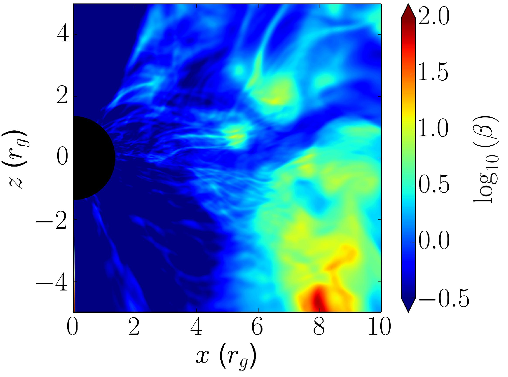

5.1 Electron Parameter Choices
Here we describe physically motivated estimates of the electron heating fraction, , and the electron thermal diffusivity, , appropriate for low-collisionality accretion flows such as that of Sagittarius A*. A more comprehensive exploration of physical models will be explored in future work.
We consider two simple models for the electron heating fraction . The first sets , a constant. Because the electron adiabatic index is not the same as the proton (total) adiabatic index, and the heating is not spatially uniform, a constant model does not necessarily lead to a constant . The second, more physical model, sets based on theoretical models of the dissipation of MHD turbulence in low-collisionality plasmas. These generically predict that electrons receive most of the turbulent heating at low while protons receive most of the turbulent heating at high . This is true both for reconnection (Numata & Loureiro, 2015) and collisionless damping of turbulent fluctuations (Quataert & Gruzinov, 1999). This dependence on is the key qualitative feature of our chosen model of . For concreteness, we use the specific calculations of Howes (2010) who provided a simple fitting function for the electron to proton heating rate as a function of plasma parameters in calculations of the collisionless damping of turbulent fluctuations in weakly compressible MHD turbulence like that expected in accretion discs. These models do a reasonable job of explaining the measured proton and electron heating rates in the near-Earth solar wind (Howes, 2011). The functional form of is derived from the relations:
| (48) |
with , , and for , while and for . The corresponding result for is simply
| (49) |
The critical assumption used in deriving equation (48) is that the turbulent fluctuations on the scale of the proton Larmor radius have frequencies much lower than the proton cyclotron frequency. This is believed to be well-satisfied for weakly compressible MHD turbulence in accretion disks (e.g., Quataert 1998). For concreteness, we note that for and , we have , while for and , , respectively. This demonstrates the strong transition from predominantly electron to predominantly proton heating with increasing , with the transition happening at a value of that depends weakly on the proton to electron temperature ratio. This implies that we expect strong electron heating in the corona and jet regions but suppressed electron heating in the bulk of the disc.
We reiterate that the key feature of equation (48) is not the precise value of the predicted , but rather the transition from for to for . This qualitative transition is much more robust than the specific functional form in equation (48) (e.g., Quataert & Gruzinov 1999; Numata & Loureiro 2015).
For the electron thermal diffusion parameters, since is a diffusion coefficient, we assume that it has the form
| (50) |
where is a dimensionless thermal diffusivity, and is the radial distance from the center of the black hole, which is comparable to the density scale height of the disc, . Since we are interested in fairly relativistic electrons, we choose the relevant velocity to be in our diffusivity estimate. In what follows, we consider a range of dimensionless diffusivities, . A typical value of is motivated by the idea that particles scatter roughly after moving a distance comparable to the length-scale over which the magnetic field strength, density, etc. change. In fact, for high beta plasmas, the mean free path due to wave-particle scattering can be significantly lower, reducing the thermal diffusivity significantly. In Appendix B.2 we discuss the specific limits imposed by electron temperature anisotropy instabilities present in a turbulent plasma. In particular, the whistler and firehose instabilities lead to limits on (eq. 66) and thus the electron viscosity and thermal diffusivity, where the temperature anisotropy is defined with respect to the local magnetic field. In terms of the electron thermal diffusivity, this becomes , where is set by velocity space instabilities and is estimated in Appendix B.2. Finally, we choose the relaxation time scale, to be given by the thermal time scale:
| (51) |
Comparing this to the stability condition given by equation (36), we see that stability is ensured if
| (52) |
Since we have a non-uniform grid, the time step is essentially set by the light crossing time of the smallest grid cell (i.e. that nearest the horizon), meaning that near the horizon and further from the horizon. For a reasonable choice of a CFL number of 0.5, we find that equation (52) is satisfied everywhere and is not a limiting factor in our simulation. Moreover, we find that the exact value of is not critical as long as it satisfies numerical stability and is not too long (e.g. is less than a local dynamical time).

5.2 Electron Heating Only
In this section we focus solely on the effects of separately evolving the electron internal energy equation without conduction in our black hole torus simulation and compare the results for different electron heating models.
5.2.1 Constant Electron Heating Fraction
Figure 8 shows the temperature ratio, , averaged over the interval for . We reiterate that here is the temperature inferred from the underlying single fluid GRMHD solution (approximately the proton temperature in our model) while is the electron temperature determined from our separate electron entropy equation. We include this constant result primarily because it is conceptually similar (although quantitatively different) to the constant assumption often used in the literature. Notice that the resulting ratio, seen in Fig. 8, is non-uniform despite the constant . Also note that due to the fact that MHD turbulence is unsustainable in 2D simulations, the heating dies off after of evolution and prevents the outer region of the disc from ever being heated substantially. However, as we will see later, conduction can occur at a much faster (electron thermal) speed along the magnetic field lines and can affect the solution at somewhat larger radii.

5.2.2 -Dependent Electron Heating
Figure 9 shows the temperature ratio, , the electron temperature itself, , and the electron heating fraction, , averaged over the interval for the -dependent heating model of equation (48), which we regard as a more physical electron heating model than const. We note that this leads to hot electrons being strongly concentrated in the corona of the torus in between the disc and the jet, where is the smallest (and from equation 48). This is also clear from the 1D profiles of electron temperature as a function of polar angle in Figure 10.
Figure 10 shows the mass-weighted average over radius () of the electron and gas temperatures, plotted versus the polar angle, . The electrons and total gas temperatures have mild variation in with , while the electrons have significantly higher temperatures in the polar regions. This demonstrates that the non-uniformity of the electron temperature in the model is primarily caused by the strong -dependence of our model of as opposed to any non-uniformity of the heating rate itself (Figure 6).


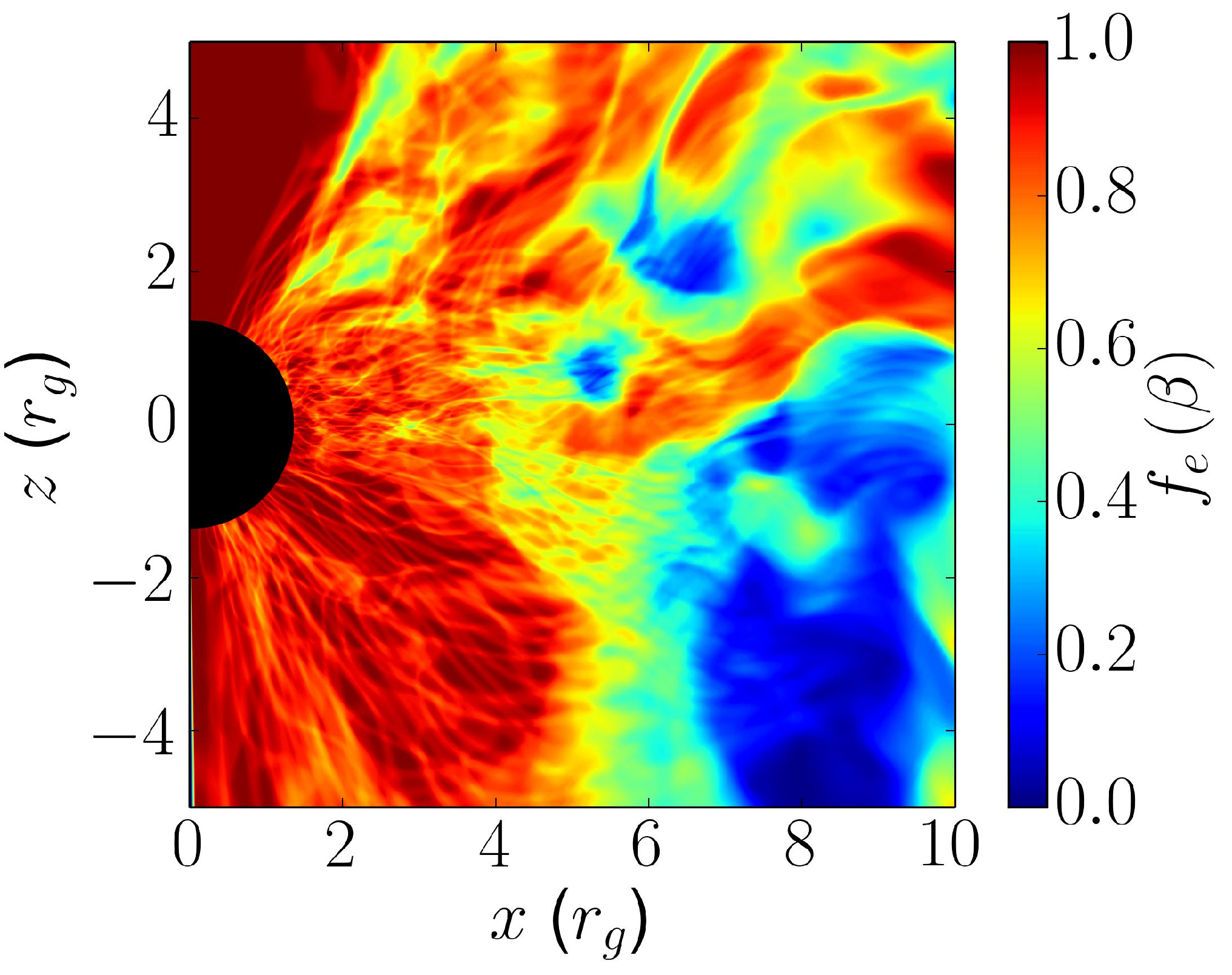

5.3 Conduction and Electron Heating
We now consider the effects of electron conduction on the electron temperature structure of black hole accretion discs. We focus on the more physical model of dependent heating described in §5.1. In all of our calculations, we include the velocity space instability limit on the electron thermal conductivity (Appendix B.2), although runs without this limit produce similar results because is modest () in the inner regions of these simulations (Figure 6). Figure 11 shows the electron temperature as a function of radius at the mid-plane in the simulations with and without conduction. Figure 12 shows the effects of conduction more quantitatively via the fractional change in temperature between the electron temperature solution with conduction and that without.
To summarise Figures 11 and 12, conduction has little effect on the electron temperature for . However, for , conduction leads to a significant radial redistribution of heat such that the electron temperature is factors of a few larger at large radii. Even for , however, the angular redistribution of heat is much less efficient, as seen in the radially and time-averaged electron temperatures in Figure 10 for . This is primarily because of the structure of the magnetic field, as can be seen by noting that the regions where conduction modifies the temperature in Figure 12 largely follow magnetic field contours which do not efficiently connect the polar and equatorial regions. To aid the interpretation of these results, Figure 13 shows the heat flux normalised to the maximum value ; even for the heat flux is still well below the saturated value in significant parts of the domain. We now summarise and interpret these results in more detail.
For we find conduction to have only a small effect on the electron thermodynamics in the accretion disc, despite the relatively high conductivity. We can understand this result as being due to the suppression of the isotropic heat flux by being projected along field lines, quantified by the ratio,
| (53) |
where and are evaluated using the electron temperature as evolved without conduction and which we now define. For this diagnostic, we use
| (54) |
where is the projection tensor that projects along a space-like direction perpendicular to the fluid velocity . This projection ensures that the heat flux in the fluid frame has a zero time-component. Likewise, for , we use the first order anisotropic heat flux: . Note that in equation (53), is always because both heat fluxes are mutually orthogonal to . Figure 14 shows in our torus simulation, where we find the suppression of the isotropic heat flux to be around . The simplest explanation for this small number is that the field is predominantly in the direction, where the temperature gradient is identically 0 in 2D simulations. For instance, in local shearing box calculations, Guan et al. (2009) found that the typical angle between and was , corresponding to a suppression of the heat flux with .
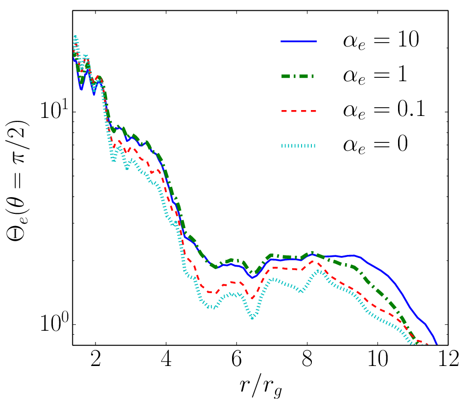


Contrary to the cases, setting causes conduction to have a significant effect by redistributing the electron heat from the coronal regions to the bulk of the torus at larger radii. This redistribution of heat causes the electron temperature to actually exceed the total gas temperature in certain regions, which formally violates our assumption that .
While the calculation with , or with , might seem to use an unphysically large conductivity, roughly corresponding to a length scale for conduction of , where is the disc density scale height, the heat flux in these calculations is limited to be smaller than the value set by the physically motivated whistler criterion in equation (67) and to be less than the saturated heat flux . As Figure 13 shows, the heat flux is saturated in only part of the domain. Furthermore, the appropriate length scale for conduction should be the scale height along field lines, which could be significantly greater than the overall density scale height if the field has a large toroidal component. For these reasons, we believe that the larger solutions may in fact be physical because they correspond to a heat flux closer to the saturated value expected in low-collisionality plasmas.
6 Conclusions
We have presented a method for evolving a separate electron entropy equation in parallel to the standard equations of ideal General Relativistic MHD. Our motivation is the study of two-temperature radiatively inefficient accretion flows (RIAFs) onto black holes, in which the electron-proton Coulomb collision time is sufficiently long that the proton and electron thermodynamics decouple (e.g., Rees et al. 1982). Understanding the electron temperature distribution close to the black hole is necessary for robustly predicting the radiation from the numerical simulations of black hole accretion (and outflows) in the sub-Eddington regime.
The long-term goal of the present work is to incorporate the key processes that influence the electron thermodynamics in RIAFs into GRMHD simulations: heating, thermal conduction, radiative cooling, and electron-proton Coulomb collisions. In the present paper we have focused on the first two of these processes. Specifically, we have developed, implemented, and tested a model that quantifies the rate of heating in a conservative GRMHD simulation (§2). We then assign a fraction of this heating to the electrons based on a microphysical model of the key heating processes (e.g., turbulence, reconnection, shocks; see, e.g., §5.1). In addition, we have implemented and tested a model of relativistic anisotropic conduction of heat (by electrons) along magnetic field lines, based on the Chandra et al. (2015) formulation of anisotropic relativistic conduction (§2.3). The electron thermal diffusivity is a free parameter in this calculation. For the black hole accretion disc applications of interest, we advocate a ‘saturated’ heat flux in which the thermal diffusivity is , subject to additional constraints imposed by velocity space instabilities and scattering by wave-particle interactions (Appendix B.2).
We implemented our electron energy model in a conservative GRMHD code HARM2D (Gammie, McKinney & Tóth, 2003), though the model we have developed can be applied to any underlying GRMHD scheme. For simplicity, the implementation in this paper neglects the back reaction of the electron pressure on the dynamics of the accretion flow. We believe that this is a reasonable first approximation given some of the uncertainties in the electron physics. Formally, this approximation is is valid only when though we expect it to be a reasonable first approximation when in regions with plasma , i.e., in the regions where gas thermal pressure forces are dynamically important.
We have demonstrated that our implementations of electron heating and conduction are accurate and second order convergent in several smooth test problems (§4 and Appendix A). For shocks, the heating converges at first order but to a post shock temperature that differs from the analytic solution by when the electron adiabatic index differs from the adiabatic index of the fluid in the GRMHD solution (e.g., Figure 2). This discrepancy arises because standard Riemann solvers ‘resolve’ the shock structure with only a few grid points. Including an explicit bulk viscosity to broaden and resolve the shock leads to a converged numerical solution for the post-shock electron energy that agrees with the analytic solution (Appendix C). In practice, the discrepancy between the numerical and analytic solutions for standard Riemann solvers is sufficiently accurate given other uncertainties in the electron physics. For this reason, we do not use bulk viscosity in our calculations. Moreover, strong shocks are rare and account for a negligible fraction of the dissipation in accretion disc simulations with aligned black hole and accretion disc angular momentum.
In addition to formulating and testing our electron energy equation model, we have also presented a preliminary application of these new methods to simulations of black hole accretion. Specifically, we have studied the impact of realistic electron heating and electron thermal conduction on the spatial distribution of the electron temperature in 2D (axisymmetric) simulations of black hole accretion onto a rotating black hole. We find that the resulting electron temperatures differ significantly from the assumption of a constant electron to proton temperature ratio used in previous work to predict the emission from GRMHD simulations (Mościbrodzka et al., 2009; Dibi et al., 2012; Drappeau et al., 2013); see, e.g. Figures 9-11. This is due to the strong -dependence of the electron heating fraction, , described in §5.1: electrons are preferentially heated in regions of lower , causing to be larger in the coronal regions compared to the midplane. In addition, we find that the effect of thermal conduction on the electron temperatures is suppressed by the fact that the heat flux must travel along field lines, which are predominantly toroidal and thus not aligned with the temperature gradient. Specifically, we find that electron conduction modifies the temperature distribution only if the effective electron mean free path along the magnetic field is the local radius in the flow (see Figure 12). In this case, there is a net transfer of heat from the corona to the bulk of the disc. This increases the electron temperature at larger radii by a factor of .
It is important to stress that the unsustainability of MHD turbulence in 2D simulations (e.g., Guan & Gammie 2008) limits how thoroughly we can interpret the accretion disc results presented in this paper. Since a steady state is never truly reached, the bulk of the disc retains memory of the initial conditions and only the innermost regions () develop significant turbulence. This could artificially limit the effects of electron conduction because the thermal time for relativistic electrons is and is thus substantially shorter than the local dynamical time only at large radii. Future work will use the methods developed here in 3D simulations.
It is also important to stress that, as in previous work, our results for both the gas and electron temperature are not reliable when . In these regions the ratios of and are so large that the evolution of the density and internal energy are dominated by truncation errors in the magnetic field, to which they are nonlinearly coupled by the total energy equation. This requires the use of density and internal energy floors. Because our calculation of the electron heating rate relies on quantifying the entropy changes in the underlying GRMHD solution, our predicted electron temperatures also become unreliable when . In the accretion disc simulations, this only affects the regions close to the pole where there is very little matter, not the evolution of the electrons in the bulk of the accretion disc or corona. We have specifically tested several treatments of the internal energy and density floors which produce dramatically different results in the poles but are all consistent in the higher density regions for both the fluid variables and the electron temperature.
Future applications of the methods developed in this paper will center on using our electron temperature calculations to predict the emission from accreting black holes. In particular, we hope to produce more accurate images of the radio and IR emission of Sagittarius A* (and M87) that can be used to interpret the forthcoming spatially resolved observations by the Event Horizon Telescope (Doeleman et al., 2009) and Gravity (Gillessen et al., 2010).
Acknowledgements
We thank F. Foucart for useful discussions, as well as all the members of the horizon collaboration, horizon.astro.illinois.edu, for their advice and encouragement. We also thank Dmitri Uzdensky for a useful and thorough referee report. This work was supported by NSF grant AST 13-33612 and NASA grant NNX10AD03G, and a Romano Professorial Scholar appointment to CFG. EQ is supported in part by a Simons Investigator Award from the Simons Foundation and the David and Lucile Packard Foundation. MC is supported by the Illinois Distinguished Fellowship from the University of Illinois. Support for AT was provided by NASA through Einstein Postdoctoral Fellowship grant number PF3-140131 awarded by the Chandra X-ray Center, which is operated by the Smithsonian Astrophysical Observatory for NASA under contract NAS8-03060, and by NSF through an XSEDE computational time allocation TG-AST100040 on TACC Stampede. This work was made possible by computing time granted by UCB on the Savio cluster.
References
- Anderson & Witting (1974) Anderson J. L., Witting H. R., 1974, Physica, 74, 466
- Andersson & Lopez-Monsalvo (2011) Andersson N., Lopez-Monsalvo C. S., 2011, Classical and Quantum Gravity, 28, 195023
- Baganoff et al. (2003) Baganoff F. K. et al., 2003, ApJ, 591, 891
- Balbus & Hawley (1991) Balbus S. A., Hawley J. F., 1991, ApJ, 376, 214
- Barrière et al. (2014) Barrière N. M. et al., 2014, ApJ, 786, 46
- Bourouaine et al. (2013) Bourouaine S., Verscharen D., Chandran B. D. G., Maruca B. A., Kasper J. C., 2013, ApjL, 777, L3
- Chandra, Foucart & Gammie (2015) Chandra M., Foucart F., Gammie C. F., 2015, ApJ, in prep.
- Chandra et al. (2015) Chandra M., Gammie C. F., Foucart F., Quataert E., 2015, ApJ, 810, 162
- Chandran et al. (2011) Chandran B. D. G., Dennis T. J., Quataert E., Bale S. D., 2011, ApJ, 743, 197
- Cranmer et al. (2009) Cranmer S. R., Matthaeus W. H., Breech B. A., Kasper J. C., 2009, ApJ, 702, 1604
- Davis, Stone & Pessah (2010) Davis S. W., Stone J. M., Pessah M. E., 2010, ApJ, 713, 52
- De Villiers & Hawley (2003) De Villiers J.-P., Hawley J. F., 2003, ApJ, 589, 458
- Dibi et al. (2012) Dibi S., Drappeau S., Fragile P. C., Markoff S., Dexter J., 2012, MNRAS, 426, 1928
- Doeleman et al. (2009) Doeleman S. et al., 2009, in Astronomy, Vol. 2010, astro2010: The Astronomy and Astrophysics Decadal Survey, p. 68
- Doeleman et al. (2008) Doeleman S. S. et al., 2008, Nature, 455, 78
- Drappeau et al. (2013) Drappeau S., Dibi S., Dexter J., Markoff S., Fragile P. C., 2013, MNRAS, 431, 2872
- Eckart (1940) Eckart C., 1940, Phys. Rev., 58, 919
- Fishbone & Moncrief (1976) Fishbone L. G., Moncrief V., 1976, ApJ, 207, 962
- Gammie, McKinney & Tóth (2003) Gammie C. F., McKinney J. C., Tóth G., 2003, ApJ, 589, 444
- Gary & Nishimura (2003) Gary S. P., Nishimura K., 2003, Physics of Plasmas, 10, 3571
- Gary & Wang (1996) Gary S. P., Wang J., 1996, JGR, 101, 10749
- Genzel et al. (2003) Genzel R., Schödel R., Ott T., Eckart A., Alexander T., Lacombe F., Rouan D., Aschenbach B., 2003, Nature, 425, 934
- Gillessen et al. (2010) Gillessen S. et al., 2010, in Society of Photo-Optical Instrumentation Engineers (SPIE) Conference Series, Vol. 7734, Society of Photo-Optical Instrumentation Engineers (SPIE) Conference Series, p. 0
- Gladd (1983) Gladd N. T., 1983, Physics of Fluids, 26, 974
- Guan & Gammie (2008) Guan X., Gammie C. F., 2008, ApJS, 174, 145
- Guan et al. (2009) Guan X., Gammie C. F., Simon J. B., Johnson B. M., 2009, ApJ, 694, 1010
- Hawley, Smarr & Wilson (1984) Hawley J. F., Smarr L. L., Wilson J. R., 1984, ApJ, 277, 296
- Hiscock & Lindblom (1985) Hiscock W. A., Lindblom L., 1985, prd, 31, 725
- Howes (2010) Howes G. G., 2010, MNRAS, 409, L104
- Howes (2011) Howes G. G., 2011, ApJ, 738, 40
- Ichimaru (1977) Ichimaru S., 1977, ApJ, 214, 840
- Israel & Stewart (1979) Israel S., Stewart J. M., 1979, Ann Phys, 118, 341
- Johnson & Quataert (2007) Johnson B. M., Quataert E., 2007, ApJ, 660, 1273
- Koide (2010) Koide S., 2010, ApJ, 708, 1459
- Komissarov (1999) Komissarov S. S., 1999, MNRAS, 303, 343
- Landau & Lifshitz (1975) Landau L. D., Lifshitz E. M., 1975, The classical theory of fields. Course of theoretical physics - Pergamon International Library of Science, Technology, Engineering and Social Studies, Oxford: Pergamon Press, 1975, 4th rev.engl.ed.
- Lemaster & Stone (2009) Lemaster M. N., Stone J. M., 2009, ApJ, 691, 1092
- Lynn (2014) Lynn J. W., 2014, PhD thesis, University of California, Berkeley
- Mahadevan & Quataert (1997) Mahadevan R., Quataert E., 1997, ApJ, 490, 605
- Misner, Thorne & Wheeler (1973) Misner C. W., Thorne K. S., Wheeler J. A., 1973, Gravitation. W.H. Freeman and Co.
- Mościbrodzka et al. (2014) Mościbrodzka M., Falcke H., Shiokawa H., Gammie C. F., 2014, aap, 570, A7
- Mościbrodzka et al. (2009) Mościbrodzka M., Gammie C. F., Dolence J. C., Shiokawa H., Leung P. K., 2009, ApJ, 706, 497
- Narayan et al. (1998) Narayan R., Mahadevan R., Grindlay J. E., Popham R. G., Gammie C., 1998, ApJ, 492, 554
- Narayan & Yi (1995) Narayan R., Yi I., 1995, ApJ, 444, 231
- Noble et al. (2006) Noble S. C., Gammie C. F., McKinney J. C., Del Zanna L., 2006, ApJ, 641, 626
- Noh (1987) Noh W. F., 1987, Journal of Computational Physics, 72, 78
- Novikov & Thorne (1973) Novikov I. D., Thorne K. S., 1973, in Black Holes (Les Astres Occlus), Dewitt C., Dewitt B. S., eds., pp. 343–450
- Numata & Loureiro (2015) Numata R., Loureiro N. F., 2015, Journal of Plasma Physics, 81, 023001
- Quataert (1998) Quataert E., 1998, Apj, 500, 978
- Quataert & Gruzinov (1999) Quataert E., Gruzinov A., 1999, ApJ, 520, 248
- Rees et al. (1982) Rees M. J., Begelman M. C., Blandford R. D., Phinney E. S., 1982, Nature, 295, 17
- Remillard & McClintock (2006) Remillard R. A., McClintock J. E., 2006, ARA& A, 44, 49
- Reynolds et al. (1996) Reynolds C. S., Di Matteo T., Fabian A. C., Hwang U., Canizares C. R., 1996, MNRAS, 283, L111
- Riquelme et al. (2012) Riquelme M. A., Quataert E., Sharma P., Spitkovsky A., 2012, ApJ, 755, 50
- Ryan, Dolence & Gammie (2015) Ryan B. R., Dolence J. C., Gammie C. F., 2015, ApJ, 807, 31
- Serabyn et al. (1997) Serabyn E., Carlstrom J., Lay O., Lis D. C., Hunter T. R., Lacy J. H., Hills R. E., 1997, ApjL, 490, L77
- Shapiro, Lightman & Eardley (1976) Shapiro S. L., Lightman A. P., Eardley D. M., 1976, ApJ, 204, 187
- Sharma et al. (2007) Sharma P., Quataert E., Hammett G. W., Stone J. M., 2007, ApJ, 667, 714
- Shcherbakov, Penna & McKinney (2012) Shcherbakov R. V., Penna R. F., McKinney J. C., 2012, ApJ, 755, 133
- Sironi (2015) Sironi L., 2015, ApJ, 800, 89
- Tchekhovskoy, McKinney & Narayan (2007) Tchekhovskoy A., McKinney J. C., Narayan R., 2007, MNRAS, 379, 469
- Tchekhovskoy, Narayan & McKinney (2011) Tchekhovskoy A., Narayan R., McKinney J. C., 2011, MNRAS, 418, L79
- Yuan, Quataert & Narayan (2003) Yuan F., Quataert E., Narayan R., 2003, ApJ, 598, 301
- Zhao et al. (2003) Zhao J.-H., Young K. H., Herrnstein R. M., Ho P. T. P., Tsutsumi T., Lo K. Y., Goss W. M., Bower G. C., 2003, ApjL, 586, L29
Appendix A Tests of Electron Conduction
This Appendix outlines tests of our numerical implementation of electron conduction that demonstrate that our calculations are robust and second-order accurate. The tests are taken directly from Chandra, Foucart & Gammie (2015), to which we refer the reader for more details.
A.1 Conduction Along Field Lines
This test is simply to check whether the electrons conduct heat along field lines properly. The initial conditions are a 2D, periodic box of physical size with uniform pressure and a small, density variation (and hence temperature variation) of the form:
| (55) |
The field lines are sinusoidal and given by
| (56) | ||||
derived from a scalar potential of
| (57) |
For the conduction parameters, we choose and and run the simulation for .
Figure 15 shows that the final state of the fluid is that of isothermal field lines, exactly as expected, with heat flux equilibrating the temperature along the magnetic field lines. This shows that our implementation of conduction properly limits the heat flux to be parallel to the magnetic field.


A.2 Linear Modes Test
This test checks whether our implementation of conduction gives the correct eigenmodes corresponding to Equation (19). Writing , we initialise perturbations in an otherwise uniform box about the equilibrium solution with wave number and run the simulation for one period: . The analytic solution is that the perturbations, , should obey . We choose and . We find that both and converge at second order to the analytical solution as shown in Figure 16.

A.3 1D Atmosphere in a Schwarzschild Metric
This test checks whether our implementation of the electron conduction gives the correct analytic result in a non-trivial space-time. In the Schwarzschild metric, the solution for a fluid in hydro-static equilibrium reduces to a system of two ordinary differential equations, which can be solved for any given temperature profile (see Chandra, Foucart & Gammie 2015 for details). For this test, we initialise the temperature and heat flux of the electrons to be this equilibrium solution for a purely radial field and see if the code can maintain it over a time of in a computational domain of . To compute the error, we again use the L1 norm and find 2nd order convergence for both and , as shown in Figure 17.

A.4 Relativistic Bondi Accretion
This test checks whether our implementation of the electron conduction gives the correct analytic result in a fluid with , which activates terms that were not present in the 1D atmosphere test. For the standard, spherically symmetric, steady-state Bondi solution for an accreting black hole (Hawley, Smarr & Wilson, 1984), we can solve equation (16) by numerical integration if we assume that the heat flux does not back-react on the electron temperature. For this test, we set the initial condition of the fluid variables to be the Bondi solution and the initial conditions of to be given by the solution to equation (16) with Dirichlet boundary conditions. We choose the sonic point to occur at and fix the outer boundary at a spherical radius of to have . The inner radius of the grid is inside the event horizon at . The test is whether or not the code can maintain this state over a period of . We find second order convergence of the heat flux to the analytical solution, as shown in Figure 18.

Appendix B Derivations
B.1 Total Heating Rate
This section derives the result quoted in equation (25).
First, we introduce the variable , which is equivalent to at the beginning of the time step and at the “predictor” step, but which is evolved over a time step according to:
| (58) |
We discretise equation (58) in a standard way (i.e. equation 21):
| (59) | ||||
where the square brackets indicate fluxes computed via the Riemann solver at cell interfaces and the generalisations to higher dimensions is straightforward. Note that we have dropped the in the and terms because at the beginning of the time step and at the step. We obtain the new value of entropy, , at via solving equation (59). We emphasise that is not the true entropy at but the entropy evolved according to equation (58) [or its discretised equivalent equation 59] and thus does not include any heating.
At the end of the time step (i.e. at ), we compute the “true” value of the entropy due to the full GRMHD evolution, according to the definition of :
| (60) |
Unlike , which does not include any heating, accounts for the heating as implied by the conservative evolution of the underlying GRMHD scheme. The difference is related to the heating incurred during time step , and we will use it below.
To compute the heating rate we evaluate the quantity:
| (61) | ||||
where the third equality holds because
and the first term vanishes due to conservation of mass. We evaluate eq. (61) at the time step in a discretised form by centring the time derivatives at but evaluating the prefactor at the time step:
| (62) | ||||
Now, multiplying eq. (59) by and adding the result to eq. (62), we obtain equation (25) of the main text:
| (63) |
B.2 Whistler Instability Limit on Conduction
We assume that the electrons are relativistic with . If the electrons relax to thermal equilibrium with a scattering rate , relativistic kinetic theory implies that the electron viscosity and thermal diffusivity satisfy (Anderson & Witting, 1974)
| (64) |
Velocity space instabilities set an upper limit on the electron thermal conductivity in a turbulent plasma. Physically, as the magnetic field in the accretion disc fluctuates in time, this generates pressure anisotropy, which is resisted by velocity space instabilities that isotropise the distribution function and thus limit the magnitude of the thermal diffusivity. Chandra et al. (2015) show that the theory of relativistic anisotropic viscosity implies that the pressure anisotropy and scattering rate are related by
| (65) |
where and we have neglected some general relativistic terms for simplicity.
Electrons satisfy limits on pressure anisotropy of
| (66) |
The second term on the right hand side of equation (66) is a fit to the whistler instability threshold for relativistically hot electrons (based on numerical solutions of the dispersion relation derived in Gladd 1983). The coefficient in the numerator technically depends weakly on , varying from for non-relativistic electrons to for (Lynn, 2014). Note that the slope of the term for the whistler instability in equation (66) is a fit for . Gary & Wang (1996) and Sharma et al. (2007) found a somewhat shallower slope in non-relativistic calculations but this is not a good fit over the large dynamic range of considered here. The first limit in equation (66) is the electron firehose instability which is an electron-scale resonant analogue of the fluid firehose instability (Gary & Nishimura, 2003). This limit is based on non-relativistic calculations and should to be extended to the relativistic limit in future work. However, based on our whistler calculations this is unlikely to be a significant effect.
Sharma et al. (2007) found that the typical pressure anisotropy satisfied in simulations that explicitly evolved a pressure tensor. Physically, this sign of the pressure anisotropy corresponds to outward angular momentum transport. Assuming that the RHS of equation (65) is , the whistler instability limit in equation (66) thus implies . This is not a significant constraint on the conductivity relative to the saturated value (), for , which can occur either in the corona/outflow or because . However, this estimate does suggest that the electron conductivity may be modest in the bulk of the disc at if .
Equation (66) can be implemented by calculating using equation (65) given an assumed (and using equation (64) to relate and ). If equation (66) is violated, should be increased and decreased such that equation (66) is satisfied. Alternatively, an even simpler first approximation would be to simply limit
| (67) |
motivated by the estimate in the preceding paragraph for the whistler instability. This is the limit we have used in the accretion disc simulations in §5 of the main text.
B.3 Electron Conduction Numerical Stability
Non-relativistically, an explicit implementation of thermal conduction is stable only if the time step, , satisfies the condition , where is the grid spacing in 1-dimension and is the thermal diffusivity. The relativistic theory outlined in , however, where the heat flux is evolved according to equation (16), differs from the non-relativistic case in that it is no longer diffusive. This alters the criterion for stability to be a condition on the relaxation time, , given by equation (36), which we derive here.
To check the numerical stability of our conduction theory we assume that we are in Minkowski space in the rest frame of the fluid, and further simplify our analysis to one dimension in which .
Under these assumptions, a Von Neumann stability analysis on equations (16) and (5) leads to a quadratic equation for the amplification factor, , with the following solutions:
| (68) | ||||
with the condition for stability being that . Here, as before, denotes the Courant factor. To analyse equation (68), we consider two cases: 1) when the square root term is real, and 2) when the square root term is imaginary.
When the square root term is real, the condition for stability becomes:
| (69) |
The right hand side is a maximum for modes, which gives, simply:
| (70) |
The more interesting case is when the square root term in Equation (68) is imaginary, where the criterion for stability becomes:
| (71) |
which, defining , has a maximum at
| (72) |
if
| (73) | ||||
and a maximum at otherwise. So if , our criterion becomes:
| (74) |
Finally, if , then we have
| (75) | ||||
The general behaviour of Equation (75) is complicated, but the result is roughly consistent with
| (76) |
for most reasonable choices of the Courant factor. This is the result quoted in equation (36) of the main text.
B.4 Electron Heating in a 1D Shock
Formally, for an ideal shock in a zero-viscosity fluid there is no unique path in space that connects the pre and post-shock values given by the Rankine-Hugoniot conditions, meaning that the dissipation per unit volume, , is not a well-defined quantity. However, by introducing any non-zero viscosity, the degeneracy is broken and there exists a unique path in space and hence a well-defined dissipation. To see this, we take the 1D Rankine-Hugoniot relations for a static shock, given some prescription for the viscous stress, ( is the dynamic viscosity coefficient, and can be an arbitrary function of plasma parameters),
| (77) | ||||
where , , and are constants representing the mass, momentum, and energy flux across the shock. Absent , we could combine these three equations in several different ways to get a relationship of the form . With non-zero viscosity, however, there is only one unique way to do this, namely, by taking and solving for , which gives:
| (78) |
or, in terms of ,
| (79) |
We assume that the electrons receive a constant fraction of the total heat:
| (80) | ||||
or in quasi-conservative form (using the mass continuity equation and assuming a flat space metric):
| (81) |
The final electron entropy is given by integrating this equation from the initial to the final density, which, for a 1D shock reduces to
| (82) |
giving:
| (83) | ||||
where is determined from the Rankine-Hugoniot conditions. For a strong shock with Mach number , this simplifies to
| (84) |
where is the pre-shock fluid velocity in the shock’s rest frame. Dividing by yields equation 41.
Appendix C Electron Heating in a Viscous Shock
In this appendix we show that by introducing an explicit bulk viscosity to the non-relativistic hydrodynamic equations, our electron heating calculation outlined in §3.3 give an electron internal energy that converges to the analytic result derived in Appendix B.4 for electron heating at a shock.
We treat viscosity by explicitly adding the 1D viscous energy and momentum fluxes to the ideal MHD fluxes for a constant kinematic viscosity, :
| (85) | |||
Note that these are non-relativistic fluxes which are formally inconsistent with the relativistic code in which they are used. However, our goal here is simply to show that with a resolved shock structure the electron heating calculation converges to the correct answer. The non-relativistic limit is fine for this purpose. The fluxes in equation (85) smooth out discontinuities to a continuous profile of finite width, determined by and the velocity scale. The solution for the profile of a viscous shock, now defined as a smooth transition from an initial to final state as opposed to a discontinuity, can be computed analytically for a constant kinematic viscosity, . In the shock frame, taking as the initial state, this solution takes the form:
| (86) |
where is the pre-shock Mach number, is the pre-shock speed at , and is a constant determining the location of the shock. For a pre-shock density , the density profile is obtained from the mass conservation equation: , which determines the pressure profile from equation (78). Similarly, the profile for the internal energy of the electrons in terms of is given by equation (83) with the substitution .
For our numerical test, we do not use the standard Noh test as outlined in §4.1.2 due to the problems noted by the original paper (Noh, 1987). For any numerical scheme that gives the shock a finite width, the formation of the shock from the converging flow undershoots the density at the center of the grid by a finite amount that does not disappear at higher resolution. Given this difficulty, our numerical test is instead to set the initial and boundary conditions of both the fluid and electron variables equal to the analytic solution for a stationary shock (e.g., equation 86) and evolve for a dynamical time of , where is the grid size. We choose , , , and . Figure 19 shows both the density profile and the ratio of the electron internal energy to the total internal energy for both and electrons at the end of the run as compared to the analytic solution (equation 83). We find good agreement with the analytic solution and second order convergence (Figure 20) up to the resolution at which relativistic errors in the analytic solution become important ().


Appendix D Torus Initial Conditions
In this appendix we describe in more detail the initial configuration of the torus in our simulations of an accreting black hole. In all expressions that follow we measure radii in units of the gravitational radius (or equivalently set ).
Fishbone & Moncrief (1976) derived an equilibrium solution (their equation 3.6) of the general relativistic hydrodynamic equations in the Kerr metric in terms of the relativistic enthalpy, , and the constant angular momentum per unit mass, . We use their equation 3.6 exactly as presented when and when the right-hand side is positive, otherwise we set . Additionally, we assume an adiabatic equation of state, , for some choice of , and fix such that the density maximum occurs at :
| (87) | ||||
where is the dimensionless spin parameter of the black hole. This expression for is equivalent to the Keplerian value at .