跳到论文正文
W Papers独立论文阅读器 arXiv:1509.04585 论文正文 计算阅读时间 · 0%
引用这篇论文根据当前论文元数据生成,正式投稿前建议核对。


License: arXiv.org perpetual non-exclusive license
arXiv:1509.04585v1 [math.DG] 15 Sep 2015

Classification of polytope metrics and complete scalar-flat Kähler 4-Manifolds with two symmetries

September 2015
Abstract

We study unbounded 2-dimensional metric polytopes such as those arising as Kähler quotients of complete Kähler 4-manifolds with two commuting symmetries and zero scalar curvature. Under a mild closedness condition, we obtain a complete classification of metrics on such polytopes, and as a result classify all possible metrics on on the corresponding Kähler 4-manifolds. If the polytope is the plane or half-plane then only flat metrics are possible, and if the polytope has one corner then the 2-parameter family of generalized Taub-NUTs (discovered by Donaldson) are indeed the only possible metrics. Polytopes with n≥3n\geq 3 edges admit an (n+2)(n+2)-dimensional family of possible metrics.

1 Introduction

We study polytope metrics of the kind arising from the reduction of complete Kähler 4-manifolds with a pair of commuting holomorphic Killing fields 𝒳1\mathcal{X}_{1}, 𝒳2\mathcal{X}_{2} and zero scalar curvature; we are particularly interested in the case that M4M^{4} is complete. In the simply-connected case, real-holomorphic fields are generated by potentials; here these are functions φi\varphi^{i} with

ω⁡(𝒳i,⋅)=−d​φi.\displaystyle\omega(\mathcal{X}_{i},\,\cdot)\;=\;-d\varphi^{i}. (1)

This leads to the so-called moment map Φ:M4↦ℝ2\Phi:M^{4}\mapsto\mathbb{R}^{2} given by Φ⁡(p)=(φ1​(p),φ2​(p))\Phi(p)=(\varphi^{1}(p),\varphi^{2}(p)), whose image is a polytope called the associated moment polytope [11][28][5][21], which we call Σ2\Sigma^{2}. Since the 𝒳i\mathcal{X}_{i} are Killing the map Φ:M2→Σ2\Phi:M^{2}\rightarrow\Sigma^{2}, which is generically submersive, endows Σ2\Sigma^{2} with a Riemannian metric gΣg_{\Sigma}; the result is a metric polytope (Σ2,gΣ)(\Sigma^{2},g_{\Sigma}) called the Kähler reduction of (M4,J,ω,𝒳1,𝒳2)(M^{4},J,\omega,\mathcal{X}_{1},\mathcal{X}_{2}). Setting

𝒱=|𝒳1|2​|𝒳2|2−⟨𝒳1,𝒳2⟩2=|∇φ1|2​|∇φ2|2−⟨∇φ1,∇φ2⟩2\displaystyle\begin{aligned} \mathcal{V}&\;=\;|\mathcal{X}_{1}|^{2}|\mathcal{X}_{2}|^{2}-\left<\mathcal{X}_{1},\,\mathcal{X}_{2}\right>^{2}\;=\;|\nabla\varphi^{1}|^{2}|\nabla\varphi^{2}|^{2}-\left<\nabla\varphi^{1},\,\nabla\varphi^{2}\right>^{2}\end{aligned} (2)

and letting △Σ\triangle_{\Sigma} be the laplacian on (Σ2,gΣ)(\Sigma^{2},g_{\Sigma}), we shall see that

△Σ​𝒱+12​s​𝒱= 0\displaystyle\triangle_{\Sigma}\sqrt{\mathcal{V}}\;+\;\frac{1}{2}s\sqrt{\mathcal{V}}\;=\;0 (3)

where ss is the scalar curvature on M4M^{4}, expressed, with 𝒱\sqrt{\mathcal{V}} as a function on Σ2\Sigma^{2}. This is a version of the Abreu equation from [1]; see the discussion in Section 2. When s=0s=0 we have a Laplace equation and 𝒱\sqrt{\mathcal{V}} is a natural harmonic coordinate on Σ2\Sigma^{2}.

Our work involves only the metric polytopes themselves, whether or not they come from any Kähler reduction. For this reason we take the time to state our hypotheses in a strictly analytic framework, apart from any Kähler geometry it may be reduced from. Unless specifically stated otherwise, we shall always assume our polytopes (Σ2,gΣ)(\Sigma^{2},g_{\Sigma}) satisfy

  • A)

    (Closedness) Σ2\Sigma^{2} is a closed subset of the (φ1,φ2)(\varphi^{1},\varphi^{2}) coordinate plane.

  • B)

    (Boundary connectedness) The polytope boundary has just one component or no components.

  • C)

    (Natural polytope condition) Σ2\Sigma^{2} is a convex polytope with finitely many edges. The metric gΣg_{\Sigma} is C∞C^{\infty} up to boundary segments and Lipschitz at corners, and each boundary segment or ray is totally geodesic.

and our functions φ1\varphi^{1}, φ2\varphi^{2} satisfy

  • D)

    (Natural boundary conditions) The unit vector fields ∇φi|∇φi|\frac{\nabla\varphi^{i}}{|\nabla\varphi^{i}|} are well-defined and covariant-constant on boundary segments.

  • E)

    (Pseudo-toric condition) The functions φ1\varphi^{1}, φ2\varphi^{2} are C∞C^{\infty} and [∇φ1,∇φ2]=0[\nabla\varphi^{1},\nabla\varphi^{2}]=0 on (Σ2,gΣ)(\Sigma^{2},g_{\Sigma}).

  • F)

    (Pseudo-ZSC condition) With 𝒱=|∇φ1|2​|∇φ2|2−⟨∇φ1,∇φ2⟩\mathcal{V}=|\nabla\varphi^{1}|^{2}|\nabla\varphi^{2}|^{2}-\left<\nabla\varphi^{1},\nabla\varphi^{2}\right>, we have △Σ​𝒱=0\triangle_{\Sigma}\sqrt{\mathcal{V}}=0.

Conditions (C), (D), and (E) are automatic when (Σ2,gΣ)(\Sigma^{2},g_{\Sigma}) is the Kähler reduction of some M4M^{4} (see §2.6). Condition (F) is simply that M4M^{4} also has zero scalar curvature.

Conditions (A) and (B), however, are genuine restrictions in the sense that there exist manifolds (M4,J,ω,𝒳1,𝒳2)(M^{4},J,\omega,\mathcal{X}_{1},\mathcal{X}_{2}) with associated polytopes that violate either or both; see Examples 7 and 8 below. We will not discuss such polytopes, except to say that (A) is violated when some symmetry has a “zero at infinity” as in Example 7, and (B) is violated when the zero locus {𝒳1=0}∪{𝒳2=0}\{\mathcal{X}_{1}=0\}\cup\{\mathcal{X}_{2}=0\} is disconnected, as in Example 8. For a discussion of why these cases are more difficult, and remain unresolved, see the final remark in Section 5.

We completely classify polytope metrics under conditions (A)-(F). Should (Σ2,gΣ)(\Sigma^{2},g_{\Sigma}) be a Kähler reduction, it is well-known that all data on M4M^{4} can be reconstructed from gΣg_{\Sigma} (see §2), so obviously our theorems about (Σ2,gΣ)(\Sigma^{2},g_{\Sigma}) have profound implications for Kähler manifolds (M4,J,ω,𝒳1,𝒳2)(M^{4},J,\omega,\mathcal{X}_{1},\mathcal{X}_{2}) with commuting symmetries.

Theorem 1.1 (Compact Polytope)

If (Σ2,gΣ)(\Sigma^{2},g_{\Sigma}) is compact, and even if (F) is relaxed to △Σ​𝒱≥0\triangle_{\Sigma}\sqrt{\mathcal{V}}\geq 0, then gΣg_{\Sigma} is flat. (C.f. Corollary 2.6.)

The following corollary is well-known:

Corollary 1.2 (Compact M4M^{4} with s≤0s\leq 0)

Assume (M4,J,ω,𝒳1,𝒳2)(M^{4},J,\omega,\mathcal{X}_{1},\mathcal{X}_{2}) has s≤0s\leq 0. If the associated metric polytope (Σ2,gΣ)(\Sigma^{2},g_{\Sigma}) is compact, then M4M^{4} is flat. (C.f. Corollary 2.7.)

The simplest non-compact case is when Σ2\Sigma^{2} is metrically complete; this is the subject of our first substantial results. Note also the different sign required of ss.

Theorem 1.3 (Polytope is complete)

Assume (Σ2,gΣ)(\Sigma^{2},g_{\Sigma}) is a geodesically complete metric polytope with △Σ​𝒱≤0\triangle_{\Sigma}\sqrt{\mathcal{V}}\leq 0 (this is a relaxation of (A) and (F)). Then gΣg_{\Sigma} is flat. (C.f. Theorem 3.3.)

Corollary 1.4

Assume (M4,J,ω,𝒳1,𝒳2)(M^{4},J,\omega,\mathcal{X}_{1},\mathcal{X}_{2}) is simply connected and has s≥0s\geq 0. If the fields are no-where zero and no-where equal, then M4M^{4} is flat. (C.f. Corollary 3.4.)

Our third theorem deals with the case that Σ2\Sigma^{2} is a half-plane. Unlike the previous results, its proof requires the full strength of (A)-(F).

Theorem 1.5 (Polytope is a half-plane)

If (Σ2,gΣ)(\Sigma^{2},g_{\Sigma}) is a closed half-plane, then gΣg_{\Sigma} is flat. (C.f. Theorem 4.17.)

Corollary 1.6

Assume (M4,J,ω,𝒳1,𝒳2)(M^{4},J,\omega,\mathcal{X}_{1},\mathcal{X}_{2}) is simply connected, scalar-flat, and has associated polytope (Σ2,gΣ)(\Sigma^{2},g_{\Sigma}) with just one edge. Then M4M^{4} is flat. (C.f. Corollary 4.18.)

When 𝒳1,𝒳2\mathcal{X}_{1},\mathcal{X}_{2} have common zeros, the situation is more complicated. Since at least the papers of Donaldson [13] and Abreu–Sena-Dias [3], it has been known that if M4M^{4} is scalar-flat and has a polytope with one or more vertices, then M4M^{4} admits at least a two-parameter family of scalar flat metrics (up to homothety). As we show, when Σ2\Sigma^{2} has just one vertex, these are all such metrics: one of these metrics is flat, one is the Taub-NUT metric, and the rest are the achiral generalized Taub-NUT metrics of Donaldson (from section 6 of [13]).

Theorem 1.7 (Polytope has one vertex)

Assume (Σ2,gΣ)(\Sigma^{2},g_{\Sigma}) has a single corner, so after affine recombination of φ1\varphi^{1}, φ2\varphi^{2} we may assume Σ2\Sigma^{2} is the closed first quadrant. Up to homothety, the metric gΣg_{\Sigma} lies within a 2-parameter family of metrics (cf. Theorem 5.2).

Corollary 1.8

Under the hypotheses of Theorem 1.5, suppose also that 𝒳1\mathcal{X}_{1}, 𝒳2\mathcal{X}_{2} have a single common zero. Up to homothety, M4M^{4} has precisely a 2-parameter family of metrics which give it a metric of zero scalar curvature (cf. Corollary 5.3).

The situation of more than two edges is different still.

Theorem 1.9 (Generic case)

Assume Σ\Sigma has n≥3n\geq 3 many edges. Under conditions (A)-(F), Σ2\Sigma^{2} admits precisely an (n+2)(n+2)-parameter family of metrics. (C.f. Theorem 5.4.)

Corollary 1.10

Suppose (Σ,gΣ)(\Sigma,g_{\Sigma}) is the Kähler reduction of a manifold (M4,J,ω,𝒳1,𝒳2)(M^{4},J,\omega,\mathcal{X}_{1},\mathcal{X}_{2}), and Σ2\Sigma^{2} has n≥3n\geq 3 edges, has no edges at infinity, and has connected boundary. If M4M^{4} is scalar flat, its metric is one in a (n+2)(n+2)-parameter family of possible metrics.F (C.f. Corollary 5.5.)

We give a detailed construction of these polytope metrics in the proof of Corollary 5.5, and a detailed recipe for constructing metrics on M4M^{4} from the metric on Σ2\Sigma^{2} in §2.3. In Example 6 below, we explicitly construct all possible such metrics on those M4M^{4} whose polytope has two corners; these include the metrics on T​ℂ​P2T\mathbb{C}P^{2} such as the Eguchi-Hanson metric, and the metrics of LeBrun [29]. Of course obtaining the M4M^{4} metric from its polytope is nothing new, see [20] [1], but the method we find most helpful is a variation on what usually appears in the literature. In particular we avoid the “Kähler potential” techniques of [20] and [1], which lead to a 4th order scalar PDE, and instead use essentially equivalent system of second order PDEs.

The proofs of Theorems 1.1 and 1.3 are reasonably self-contained and easy. Theorem 1.5 requires the preparatory work of §2.5 and §2.6 and the difficult analysis of §4, which classifies non-negative solutions of x⁡(φx​x+φy​y)−φx=0x(\varphi_{xx}+\varphi_{yy})-\varphi_{x}=0 on the half-plane H2={x>0}H^{2}=\{x>0\} with zero boundary values. The geometric classifications in Theorems 1.7 and 1.10 are essentially corollaries of the analytic classification. The equation x⁡(φx​x+φy​y)−φx=0x(\varphi_{xx}+\varphi_{yy})-\varphi_{x}=0 is in fact a geometric PDE that appeared first in a paper of Donaldson’s [12]; see Proposition 2.5 and the discussion at the beginning of Section 4.

The main result of Section §4 is a Liouville-type result for the degenerate-elliptic equation x⁡(fx​x+fy​y)+3​fx=0x(f_{xx}+f_{yy})+3f_{x}=0 by combining the techniques of blow-ups, barriers, and Fourier analysis. A certain duality relation exists between x⁡(fx​x+fy​y)+3​fx=0x(f_{xx}+f_{yy})+3f_{x}=0 with arbitrary boundary conditions on the half-plane H2H^{2} and the PDE x⁡(φx​x+φy​y)−φx=0x(\varphi_{xx}+\varphi_{yy})-\varphi_{x}=0 with zero boundary conditions on H2H^{2}, so the Liouville-type theorem for the first gives the desired classification of all non-negative solutions for the second: these all have the form C​x2Cx^{2} for C>0C>0.

Degenerate-elliptic PDE have long been studied in their own right (eg. [26] [25]). The particular equations x⁡(gx​x+gy​y)+ν​gx=0x\left(g_{xx}+g_{yy}\right)+\nu{g}_{x}=0 and the corresponding parabolic equation gt=x⁡(gx​x+gy​y)+ν​gxg_{t}=x\left(g_{xx}+g_{yy}\right)+\nu{g}_{x} have been studied in a variety of contexts, almost exclusively for ν≥0\nu\geq 0 (although there is a duality between the cases ν>1\nu>1 and ν<1\nu<1: if gg solves the equation for ν\nu then g~=xν−1​g\tilde{g}=x^{\nu-1}g solves it for ν~=2−ν\tilde{\nu}=2-\nu).

The operator △μ=x⁡(∂2∂x2+∂2∂y2)\triangle_{\mu}=x\left(\frac{\partial^{2}}{\partial{x}^{2}}+\frac{\partial^{2}}{\partial{y}^{2}}\right) can be considered a Laplace operator for the right half-plane with a hypoerbolic metric. Thus from a naive point of view, gt=△μ​g+ν​gxg_{t}=\triangle_{\mu}{g}+\nu{g}_{x} can be considered a heat flow through an isotropic but inhomogeneous medium of hyperbolic specific heat density, with a directional transfer bias indicated by ν\nu. Less naively, this equation (or similar equations such as the Heston equation, equation (137)) has been studied in connection with mathematical finance, stochastic PDE and Feynman-Kac theory [22], mathematical biology [14], and the porous medium equation [10]. The change of variables s=12​x2s=\frac{1}{2}x^{2}, t=2​yt=\sqrt{2}y turns x⁡(gx​x+gy​y)−gx=0x(g_{xx}+g_{yy})-g_{x}=0 into s​fs​s+ft​t=0s{f}_{ss}+f_{tt}=0, which has been studied in connection with population dynamics [14].

However, much of this study has been related to existence/uniqueness of flows or boundary value problems, Hölder estimates, admissibility of boundary values, and so on. Much of this work has been local or confined to pre-compact domains, although there are global results such as global Hölder estimates. To this author’s knowledge, this paper contains the first Liouville-type result for these equations.

Remark. Our 4-manifolds need not be “toric” exactly, but only have commuting holomorphic Killing fields. Our work takes place mostly on the moment polytope where the vertex angles are irrelevant. There is no particular need that the momentum construction rebuild any actual 4-manifold.

Remark. Our conclusions will hold directly on certain orbifolds with commuting holomorphic Killing fields. However we do not explore the significance of our results to the situation of “marked polytopes” [30] and the like.

Remark. Notice that Theorem 1.1 requires s≤0s\leq 0 and Theorem 1.3 requires s≥0s\geq 0, but s=0s=0 is necessary for the other three theorems. We conjecture that Theorem 1.5 (that the half-plane is flat) continues to hold if s≥0s\geq 0. Further, we conjecture that if s≥0s\geq 0 is some pre-specified function, then Theorem 1.7 holds with the “up to homothety” removed. However the techniques of §4 will not work without s≡0s\equiv 0, and a more sophisticated analysis is required. See the discussion at the beginning of §4.

Remark. It is important to mention two issues not addressed in this paper. The first is the question of how many of the metrics in our (n+2)(n+2)-dimensional family are repeats. Conceivably even the dimension of this family could be reduced by the action of some diffeomorphism group, although we do not believe this to be the case.

The second is that, although the polytopes Σ2\Sigma^{2} with n≥3n\geq 3 edges have an (n+2)(n+2)-dimensional family of metrics, we do not address the issue of which of these may actually come from the reduction of some M4M^{4}. This is a another way the family of scalar-flat metrics on M4M^{4} may possibly be smaller than (n+2)(n+2)-dimensional.

Acknowledgements. The author would like to thank Xiuxiong Chen, Ryan Hynd, Philip Gressman, and Camelia Pop for a number of helpful conversations that provided some valuable insights.

2 Kähler Reduction

Here we discuss the detailed relationship between the Kähler reduction (Σ2,gΣ)(\Sigma^{2},g_{\Sigma}) and (M4,J,ω,𝒳1,𝒳2CLOSE(M^{4},J,\omega,\mathcal{X}_{1},\mathcal{X}_{2}). The philosophy is “Guillemin’s principle,” to wit, sympelctic coordinates are useful in Kähler geometry [20], [2]. This principle has been excellently developed by a number of authors [20] [1] [12] [3] [6], but begging the knowledgeable reader’s forbearance, we redevelop some aspects as suits the present interest. First we indicate this section’s primary milestones.

In §2.1 we perform the symplectic reduction itself, performing the Arnold-Liouville [4] reduction process, and relating the symplectic coordinates (φ1,φ2,θ1,θ2)(\varphi^{1},\varphi^{2},\theta^{1},\theta^{2}) to the complex-analytic coordinates (z1,z2)(z^{1},z^{2}). The resulting holomorphic volume form is a quarter of the parallelochoron volume, which is

𝒱≜|𝒳1|2​|𝒳2|2−⟨𝒳1,𝒳2⟩2=|∇φ1|2​|∇φ2|2−⟨∇φ1,∇φ2⟩2,\displaystyle\mathcal{V}\;\triangleq\;|\mathcal{X}_{1}|^{2}|\mathcal{X}_{2}|^{2}-\left<\mathcal{X}_{1},\mathcal{X}_{2}\right>^{2}\;=\;|\nabla\varphi^{1}|^{2}|\nabla\varphi^{2}|^{2}-\left<\nabla\varphi^{1},\nabla\varphi^{2}\right>^{2}, (4)

which implies that the scalar curvature of (M4,J,ω)(M^{4},J,\omega) is s=−△​log⁡𝒱s=-\triangle\log\mathcal{V}. Our notational set-up this well-known construction will be useful later.

Even with this elliptic relation, and even with a sign on ss, the behavior of log⁡𝒱\log\mathcal{V} on M4M^{4} may be hard to understand, and so in §2.2 we bring everything down to the metric polytope (Σ2,gΣ)(\Sigma^{2},g_{\Sigma}) itself, which is naturally a Riemannian manifold that may or may not have boundary. In the inherited metric we show △Σ​𝒱12+12​s​𝒱12=0\triangle_{\Sigma}\mathcal{V}^{\frac{1}{2}}+\frac{1}{2}s\mathcal{V}^{\frac{1}{2}}=0, which is a version of the Abreu equation: see (10) of [1]. Of course when M4M^{4} is scalar-flat then 𝒱\sqrt{\mathcal{V}} is harmonic on (Σ2,gΣ)(\Sigma^{2},g_{\Sigma}), and we have natural isothermal coordinates (x,y)(x,y) on Σ2\Sigma^{2} where x=𝒱x=\sqrt{\mathcal{V}} and yy is defined by JΣ​d​y=d​xJ_{\Sigma}{d}y=dx. We compute the Gauss curvature KΣK_{\Sigma} of Σ2\Sigma^{2} in these coordinates.

In §2.3 we show how to reconstruct the metrics gΣg_{\Sigma}, gg simply by knowing φ1\varphi^{1}, φ2\varphi^{2} as functions of (x,y)(x,y). We also compute the intrinsic Gaussian curvature KΣK_{\Sigma} of (Σ2,gΣ)(\Sigma^{2},g_{\Sigma}) in a second, independent way, and show that although KΣK_{\Sigma} is not necessarily signed, after a canonical conformal change it is indeed signed.

In §2.5 we prove the isothermal coordinate system (x,y)(x,y) actually has no critical points, and that the map X=(x,y)TX=(x,y)^{T} sends Σ2\Sigma^{2} onto the right half-plane {x≥0}\{x\geq 0\} in a one-to-one fashion, and the isothermal coordinates are therefore global. This fundamentally relies on condition (B), connectedness of the polytope boundary.

Finally in §2.6 we partially control the behaviors of φ1\varphi^{1}, φ2\varphi^{2}, xx, and yy near the polytope edges. This provides us with boundary conditions that are necessary to our analysis of §4 and also to our penultimate construction, in Theorem 5.4.

2.1 Fundamentals

We have a simply connected Kähler 4-manifold with commuting Killing fields (M4,J,ω,𝒳1,𝒳2)(M^{4},J,\omega,\mathcal{X}_{1},\mathcal{X}_{2}). The momentum construction consists of finding potentials φ1\varphi^{1}, φ2\varphi^{2} satisfying ω⁡(𝒳i,⋅)=−d​φi\omega(\mathcal{X}_{i},\cdot)=-d\varphi^{i}, traditionally called momentum variables or action coordinates. Two additional coordinates θ1\theta^{1}, θ2\theta^{2}, called cyclic variables or angle coordinates, are defined by taking a transversal to the {𝒳1,𝒳2}\{\mathcal{X}_{1},\mathcal{X}_{2}\} distribution and then pushing the natural ℝ2\mathbb{R}^{2} variables forward along the action of {𝒳1,𝒳2}\{\mathcal{X}_{1},\mathcal{X}_{2}\}. Obviously the values of θ1\theta^{1}, θ2\theta^{2} are not canonical, but the fields ∂∂θ1\frac{\partial}{\partial\theta^{1}}, ∂∂θ2\frac{\partial}{\partial\theta^{2}} are canonical. This construction gives a full coordinate system {φ1,φ2,θ1,θ2}\{\varphi^{1},\varphi^{2},\theta^{1},\theta^{2}\} with fields

∂∂φ1=|𝒳2|2𝒱∇φ1−⟨𝒳1,𝒳2⟩𝒱∇φ2,∂∂θ1=𝒳1,∂∂φ2=−⟨𝒳1,𝒳2⟩𝒱∇φ1+|𝒳1|2𝒱∇φ2,∂∂θ2=𝒳2.\displaystyle\begin{array}[]{ll}\frac{\partial}{\partial\varphi^{1}}\;=\;\frac{\left|\mathcal{X}_{2}\right|^{2}}{\mathcal{V}}\,\nabla\varphi^{1}\,-\,\frac{\left<\mathcal{X}_{1},\,\mathcal{X}_{2}\right>}{\mathcal{V}}\,\nabla\varphi^{2},&\frac{\partial}{\partial\theta^{1}}\;=\;\mathcal{X}_{1},\\ \\ \frac{\partial}{\partial\varphi^{2}}\;=\;-\frac{\left<\mathcal{X}_{1},\,\mathcal{X}_{2}\right>}{\mathcal{V}}\,\nabla\varphi^{1}\,+\,\frac{\left|\mathcal{X}_{1}\right|^{2}}{\mathcal{V}}\,\nabla\varphi^{2},&\frac{\partial}{\partial\theta^{2}}\;=\;\mathcal{X}_{2}.\end{array}

Letting G−1G^{-1} be the matrix

G−1=(|𝒳1|2⟨𝒳1,𝒳2⟩⟨𝒳1,𝒳2⟩|𝒳2|2),\displaystyle G^{-1}\;=\;\left(\begin{array}[]{cc}|\mathcal{X}_{1}|^{2}&\left<\mathcal{X}_{1},\,\mathcal{X}_{2}\right>\\ \left<\mathcal{X}_{1},\,\mathcal{X}_{2}\right>&|\mathcal{X}_{2}|^{2}\end{array}\right),

then the ordered frame ∂∂φ1,∂∂φ2,∂∂θ1,∂∂θ2\frac{\partial}{\partial\varphi^{1}},\frac{\partial}{\partial\varphi^{2}},\frac{\partial}{\partial\theta^{1}},\frac{\partial}{\partial\theta^{2}} produces the metric, complex structure, and symplectic form

g=(G00G−1),J=(0−G−1G0),ω=(0−I​dI​d0).\displaystyle g\;=\;\left(\begin{array}[]{c|c}G&0\\ \hline\cr 0&\;\;G^{-1}\end{array}\right),\quad J\;=\;\left(\begin{array}[]{c|c}0&-G^{-1}\\ \hline\cr\;G&0\end{array}\right),\quad\omega\;=\;\left(\begin{array}[]{c|c}0&\;-Id\\ \hline\cr Id&0\end{array}\right).

Remark. Compare (2.1) to compare (4.8) of [20] or (2.2), (2.3) of [2]. The more usual construction sets G=∇2uG=\nabla^{2}\,u for a function uu called the Kähler potential. In the present work we do not find this formulation useful. In our formulation, of course it may be objected that expressing the metric in terms of inner products is redundant. Still, this formulation lends itself to the study of second order instead of fourth order PDEs, and is useful in relating the polytope metric gΣg_{\Sigma} with the original metric gg.

Lemma 2.1 (Symplectic and holomorphic coordinates on M4M^{4})

The complex-valued functions

z1=f1​(φ1,φ2)+−1​θ1z2=f2​(φ1,φ2)+−1​θ2\displaystyle\begin{aligned} z^{1}&\;=\;f^{1}(\varphi^{1},\,\varphi^{2})\,+\,\sqrt{-1}\,\theta^{1}\\ z^{2}&\;=\;f^{2}(\varphi^{1},\,\varphi^{2})\,+\,\sqrt{-1}\,\theta^{2}\end{aligned} (19)

form a holomorphic coordinate chart provided f1f^{1}, f2f^{2} satisfy

d​f1=J​d​θ1=|𝒳2|2𝒱​d​φ1−⟨𝒳1,𝒳2⟩𝒱​d​φ2d​f2=J​d​θ2=−⟨𝒳1,𝒳2⟩𝒱​d​φ1+|𝒳1|2𝒱​d​φ2.\displaystyle\begin{aligned} &df^{1}\;=\;Jd\theta^{1}\;=\;\frac{|\mathcal{X}_{2}|^{2}}{\mathcal{V}}\,d\varphi^{1}\,-\,\frac{\left<\mathcal{X}_{1},\,\mathcal{X}_{2}\right>}{\mathcal{V}}\,d\varphi^{2}\\ &df^{2}\;=\;Jd\theta^{2}\;=\;-\frac{\left<\mathcal{X}_{1},\,\mathcal{X}_{2}\right>}{\mathcal{V}}\,d\varphi^{1}\,+\,\frac{|\mathcal{X}_{1}|^{2}}{\mathcal{V}}\,d\varphi^{2}.\end{aligned} (20)

Further, d​J​d​θi=0dJd\theta^{i}=0, so indeed such functions f1f^{1}, f2f^{2} can be found locally, and therefore holomorphic coordinates of the form (19) exist on (M4,J,ω)(M^{4},J,\omega).

Proof. Using that ∂¯=12​(d+−1​J​d)\bar{\partial}=\frac{1}{2}\left(d+\sqrt{-1}Jd\right) on functions gives that ∂¯​zi=0\bar{\partial}{z}^{i}=0 if and only if (20) holds. That d​J​d​θi=0dJd\theta^{i}=0 follows from the preservation of JJ under the action of 𝒳1\mathcal{X}_{1}, 𝒳2\mathcal{X}_{2} (a lengthy though elementary calculation can give d​J​d​θi=0dJd\theta^{i}=0 directly). □\Box

One easily determines the holomorphic frame and coframe

∂∂z1=12​(|𝒳1|2​∂∂φ1+⟨𝒳1,𝒳2⟩​∂∂φ2−−1​∂∂θ1)=12​(∇φ1−−1​𝒳1)∂∂z2=12​(⟨𝒳1,𝒳2⟩​∂∂φ1+|𝒳2|2​∂∂φ2−−1​∂∂θ2)=12​(∇φ2−−1​𝒳2)d​z1=|𝒳2|2𝒱​d​x1−⟨𝒳1,𝒳2⟩𝒱​d​x2+−1​d​θ1=J​d​θ1+−1​d​θ1d​z2=−⟨𝒳1,𝒳2⟩𝒱​d​x1+|𝒳1|2𝒱​d​x2+−1​d​θ2=J​d​θ2+−1​d​θ2\displaystyle\begin{aligned} \frac{\partial}{\partial{z}^{1}}\;=\;&\frac{1}{2}\left(|\mathcal{X}_{1}|^{2}\frac{\partial}{\partial\varphi^{1}}\,+\,\left<\mathcal{X}_{1},\,\mathcal{X}_{2}\right>\frac{\partial}{\partial\varphi^{2}}\,-\,\sqrt{-1}\,\frac{\partial}{\partial\theta^{1}}\right)\;=\;\frac{1}{2}\left(\nabla\varphi^{1}\,-\,\sqrt{-1}\,\mathcal{X}_{1}\right)\\ \frac{\partial}{\partial{z}^{2}}\;=\;&\frac{1}{2}\left(\left<\mathcal{X}_{1},\,\mathcal{X}_{2}\right>\frac{\partial}{\partial\varphi^{1}}\,+\,|\mathcal{X}_{2}|^{2}\frac{\partial}{\partial\varphi^{2}}\,-\,\sqrt{-1}\,\frac{\partial}{\partial\theta^{2}}\right)\;=\;\frac{1}{2}\left(\nabla\varphi^{2}\,-\,\sqrt{-1}\,\mathcal{X}_{2}\right)\\ dz^{1}\;=\;&\frac{|\mathcal{X}_{2}|^{2}}{\mathcal{V}}dx^{1}\,-\,\frac{\left<\mathcal{X}_{1},\,\mathcal{X}_{2}\right>}{\mathcal{V}}dx^{2}\,+\,\sqrt{-1}\,d\theta^{1}\;=\;Jd\theta^{1}\,+\,\sqrt{-1}\,d\theta^{1}\\ dz^{2}\;=\;&-\frac{\left<\mathcal{X}_{1},\,\mathcal{X}_{2}\right>}{\mathcal{V}}dx^{1}\,+\,\frac{|\mathcal{X}_{1}|^{2}}{\mathcal{V}}dx^{2}\,+\,\sqrt{-1}\,d\theta^{2}\;=\;Jd\theta^{2}\,+\,\sqrt{-1}\,d\theta^{2}\end{aligned} (21)

so in the holomorphic frame the Hermitian metric and associated volume element are simply

hi​ȷ¯=12​(|𝒳1|2⟨𝒳1,𝒳2⟩⟨𝒳1,𝒳2⟩|𝒳2|2)=12​G−1,dethi​ȷ¯=14​𝒱.\displaystyle\begin{aligned} &h_{i\bar{\jmath}}\;=\;\frac{1}{2}\left(\begin{array}[]{cc}|\mathcal{X}_{1}|^{2}&\left<\mathcal{X}_{1},\,\mathcal{X}_{2}\right>\\ \left<\mathcal{X}_{1},\,\mathcal{X}_{2}\right>&|\mathcal{X}_{2}|^{2}\end{array}\right)\;=\;\frac{1}{2}G^{-1},\\ &\det\,h_{i\bar{\jmath}}\;=\;\frac{1}{4}\mathcal{V}.\end{aligned} (22)
Proposition 2.2

The Ricci form and scalar curvature of (M4,J,ω)(M^{4},J,\omega) are

ρ=−−1∂∂¯log𝒱s=−△​log⁡𝒱.\displaystyle\begin{aligned} \rho&\;=\;-\sqrt{-1}\partial\bar{\partial}\log\,\mathcal{V}\\ s&\;=\;-\triangle\log\,\mathcal{V}.\end{aligned} (23)

Proof. Textbook formulas. □\Box

Remark. We have given, in Lemma 2.1 and (21), a very prosaic version of what is usually a expressed as a Legendre transform between the so-called Kähler and symplectic potentials, as developed in [20] (see also [1]). As we have chosen not to work with Kähler potentials, these Legendre transform methods won’t apply. In any case the workaday formulation above is probably more useful in the present context.

2.2 Reduction of M4M^{4} to a Metric Polytope

Let (Σ2,gΣ)(\Sigma^{2},g_{\Sigma}) be the Riemannian quotient (leaf space) of M4M^{4} by the Killing actions of 𝒳1\mathcal{X}_{1}, 𝒳2\mathcal{X}_{2}. The commutativity of 𝒳1\mathcal{X}_{1}, 𝒳2\mathcal{X}_{2} imply the functions φ1\varphi^{1}, φ2\varphi^{2} pass to the quotient and there constitute a coordinate system. As is well-known, the differentiable map Φ:Σ2→ℝ2\Phi:\Sigma^{2}\rightarrow\mathbb{R}^{2}, Φ⁡(p)=(φ1​(p),φ2​(p))T\Phi(p)=(\varphi^{1}(p),\varphi^{2}(p))^{T} is 1-1 with differentiable inverse, so Σ2\Sigma^{2} may be identified with its image in the (φ1,φ2)(\varphi^{1},\varphi^{2})-coordinate plane. This constitutes the moment polytope of M4M^{4}.

For clarity, objects on Σ2\Sigma^{2} will be indicated with a subscript, so for instance sΣs_{\Sigma} and ss indicate the scalar curvatures on (Σ2,gΣ)(\Sigma^{2},g_{\Sigma}) and (M4,J,ω)(M^{4},J,\omega), respectively. The inherited metric and natural complex structure are

gΣ=𝒱−1​(|𝒳2|2−⟨𝒳1,𝒳2⟩−⟨𝒳1,𝒳2⟩|𝒳1|2)=G,\displaystyle g_{\Sigma}\;=\;\mathcal{V}^{-1}\left(\begin{array}[]{cc}|\mathcal{X}_{2}|^{2}&-\left<\mathcal{X}_{1},\,\mathcal{X}_{2}\right>\\ -\left<\mathcal{X}_{1},\,\mathcal{X}_{2}\right>&|\mathcal{X}_{1}|^{2}\\ \end{array}\right)\;=\;G,
JΣ=𝒱−12​(⟨𝒳1,𝒳2⟩−|𝒳1|2|𝒳2|2−⟨𝒳1,𝒳2⟩).\displaystyle J_{\Sigma}\;=\;\mathcal{V}^{-\frac{1}{2}}\left(\begin{array}[]{cc}\left<\mathcal{X}_{1},\,\mathcal{X}_{2}\right>&-|\mathcal{X}_{1}|^{2}\\ |\mathcal{X}_{2}|^{2}&-\left<\mathcal{X}_{1},\,\mathcal{X}_{2}\right>\end{array}\right).

Of course JΣJ_{\Sigma} is not inherited from JJ, but is the Hodge star of (Σ2,gΣ)(\Sigma^{2},g_{\Sigma}).

Proposition 2.3 (Σ2\Sigma^{2} and M4M^{4} Laplacian relationship)

If f:M4→ℂf:M^{4}\rightarrow\mathbb{C} is any function on MM that is 𝒳1\mathcal{X}_{1}- and 𝒳2\mathcal{X}_{2}-invariant, then △​f\triangle{f} is 𝒳1\mathcal{X}_{1}, 𝒳2\mathcal{X}_{2} invariant, so ff, △​f\triangle{f} are naturally functions on Σ2\Sigma^{2}. As functions on Σ2\Sigma^{2}, the two Laplacians are related by

△​f\displaystyle\triangle{}f =\displaystyle= △Σ​f+⟨∇Σ​log​𝒱12,∇Σf⟩Σ\displaystyle\triangle_{\Sigma}{f}\,+\,\left<\nabla_{\Sigma}\log{\mathcal{V}}^{\frac{1}{2}},\,\nabla_{\Sigma}f\right>_{\Sigma} (30)

Proof. A function f:M4→ℂf:M^{4}\rightarrow\mathbb{C} is invariant under 𝒳1\mathcal{X}_{1}, 𝒳2\mathcal{X}_{2} if and only if it is a function of φ1\varphi^{1}, φ2\varphi^{2} only. Noting that det(g)=1\det(g)=1 and det(gΣ)=𝒱−1\det(g_{\Sigma})=\mathcal{V}^{-1} we have

△​f=∂∂φi​(gi​j​∂f∂φj)=∂∂φi​(gΣi​j​∂f∂φj)=𝒱12​∂∂φi​(gΣi​j​𝒱−12​∂f∂φj)+gΣi​j​∂log⁡𝒱12∂φi​∂f∂φj=△Σ​f+12​⟨∇Σ​log​𝒱,∇Σf⟩Σ.\displaystyle\begin{aligned} \triangle{f}&\;=\;\frac{\partial}{\partial\varphi^{i}}\left(g^{ij}\frac{\partial{f}}{\partial\varphi^{j}}\right)\;=\;\frac{\partial}{\partial\varphi^{i}}\left(g_{\Sigma}^{ij}\frac{\partial{f}}{\partial\varphi^{j}}\right)\\ &\;=\;\mathcal{V}^{\frac{1}{2}}\frac{\partial}{\partial\varphi^{i}}\left(g_{\Sigma}^{ij}\mathcal{V}^{-\frac{1}{2}}\frac{\partial{f}}{\partial\varphi^{j}}\right)\;+\;\,g_{\Sigma}^{ij}\frac{\partial\log{\mathcal{V}}^{\frac{1}{2}}}{\partial\varphi^{i}}\frac{\partial{f}}{\partial\varphi^{j}}\\ &\;=\;\triangle_{\Sigma}{f}\,+\,\frac{1}{2}\left<\nabla_{\Sigma}\log\mathcal{V},\,\nabla_{\Sigma}{f}\right>_{\Sigma}.\end{aligned} (31)

□\Box

Corollary 2.4 (Second order Abreu equation)

The scalar curvature ss on M4M^{4} passes to a function on Σ2\Sigma^{2}, and

△Σ​𝒱12+12​s​𝒱12= 0.\displaystyle\triangle_{\Sigma}\mathcal{V}^{\frac{1}{2}}\,+\,\frac{1}{2}s\,\mathcal{V}^{\frac{1}{2}}\;=\;0. (32)

Proof. This follows from s=−△​log⁡𝒱s=-\triangle\log\mathcal{V} and Proposition 2.3. □\Box

Proposition 2.5 (The φi\varphi^{i} elliptic equations)

On Σ2\Sigma^{2} we have d⁡(𝒱−12​JΣ​d​φi)=0d\left(\mathcal{V}^{-\frac{1}{2}}J_{\Sigma}{d}\varphi^{i}\right)=0.

Proof. If Φ:M4→Σ2\Phi:M^{4}\rightarrow\Sigma^{2} is the moment map projection onto the polytope, then from (2.1) and (2.2) we obtain d​fi=Φ∗​(𝒱−12​JΣ​d​φi)df^{i}=\Phi^{*}(\mathcal{V}^{-\frac{1}{2}}J_{\Sigma}{}d\varphi^{i}), where the fif^{i} are from Lemma 2.1. Finally d​Φ∗=Φ∗​dd\Phi^{*}=\Phi^{*}d and the fact that Φ\Phi is a submersion gives d⁡(𝒱−12​JΣ​d​φi)=0d(\mathcal{V}^{-\frac{1}{2}}J_{\Sigma}{}d\varphi^{i})=0 □\Box

Remark. When s=0s=0, the equations 𝒱12​d​(𝒱−12​J​d​φi)=0\mathcal{V}^{\frac{1}{2}}d\left(\mathcal{V}^{-\frac{1}{2}}Jd\varphi^{i}\right)=0 are just the equations φx​xi+φy​yi−x−1​φxi=0\varphi^{i}_{xx}+\varphi^{i}_{yy}-x^{-1}\varphi^{i}_{x}=0 on the right half-plane. See Section 4.

The following simple theorem illustrates a contrast between the compact case, where s≤0s\leq 0 is impossible, and the open case (eg. Theorem 1.3), where s≤0s\leq 0 is required, at least at one point.

Corollary 2.6

If (Σ2,gΣ)(\Sigma^{2},g_{\Sigma}) is topologically compact, it is impossible that △Σ​𝒱≥0\triangle_{\Sigma}\sqrt{\mathcal{V}}\geq 0.

Proof. The maximum principle gives 𝒱=c​o​n​s​t\mathcal{V}=const. But 𝒱=0\mathcal{V}=0 on ∂Σ2\partial\Sigma^{2}, so 𝒱≡0\mathcal{V}\equiv 0. □\Box

Corollary 2.7

If (M4,J,ω,𝒳1,𝒳2)(M^{4},J,\omega,\mathcal{X}_{1},\mathcal{X}_{2}) is topologically compact, it is impossible that s≤0s\leq 0.

Proof. If s≤0s\leq 0 then △Σ​V≤0\triangle_{\Sigma}\sqrt{V}\leq 0, so the previous corollary applies. But 𝒱≡0\mathcal{V}\equiv 0 means 𝒳1\mathcal{X}_{1} and 𝒳2\mathcal{X}_{2} are co-linear throughout, an impossibility. □\Box

2.3 Reconstruction of the metric on M4M^{4} provided s=0s=0

We show how to reconstruct the metrics on (M4,J,ω)(M^{4},J,\omega) and (Σ2,gΣ)(\Sigma^{2},g_{\Sigma}) from knowledge of the functions φ1\varphi^{1}, φ2\varphi^{2}, 𝒱\mathcal{V} on Σ2\Sigma^{2}. Proposition 2.5 tells us the coordinates φi\varphi^{i} are not harmonic on (Σ2,gΣ)(\Sigma^{2},g_{\Sigma}); indeed if φ1\varphi^{1}, φ2\varphi^{2} are harmonic then gΣg_{\Sigma} and gg are both flat metrics; see Lemma 3.1. Instead, when s=0s=0, the equation △​𝒱12=0\triangle\mathcal{V}^{\frac{1}{2}}=0 shows 𝒱12\mathcal{V}^{\frac{1}{2}} and its dual harmonic function constitute a natural harmonic coordinate system. We denote these by (x1,x2)(x^{1},x^{2}), where x1x^{1} and x2x^{2} are defined as the solutions to

x1=𝒱,d​x2=JΣ​d​x1.\displaystyle x^{1}\;=\;\sqrt{\mathcal{V}},\quad\quad dx^{2}=J_{\Sigma}dx^{1}. (33)

We shall use the notations (x,y)(x,y) and (x1,x2)(x^{1},x^{2}) interchangeably. Regarding φ1\varphi^{1}, φ2\varphi^{2} as functions of (x,y)(x,y), the formula for JΣJ_{\Sigma} in (2.2) gives

1x1​⟨∇φi,∇φj⟩​d​φ1∧d​φ2=−d​φi∧JΣ​d​φj.\displaystyle\begin{aligned} &\frac{1}{x^{1}}\left<\nabla\varphi^{i},\,\nabla\varphi^{j}\right>\,d\varphi^{1}\wedge{}d\varphi^{2}\;=\;-d\varphi^{i}\wedge{}J_{\Sigma}{}d\varphi^{j}.\end{aligned} (34)

Changing variables to express both sides in terms of (x1,x2)(x^{1},x^{2}) we have

d​φ1∧d​φ2=d​φ1d​xi​d​φ2d​xj​d​xi∧d​xj=(d​φ1d​x1​d​φ2d​x2−d​φ2d​x1​d​φ1d​x2)​d​x1∧d​x2,−d​φi∧JΣ​d​φj=(d​φid​x1​d​φjd​x1+d​φid​x2​d​φjd​x2)​d​x1∧d​x2,\displaystyle\begin{aligned} d\varphi^{1}\wedge{}d\varphi^{2}&\;=\;\frac{d\varphi^{1}}{dx^{i}}\frac{d\varphi^{2}}{dx^{j}}dx^{i}\wedge{}dx^{j}\;=\;\left(\frac{d\varphi^{1}}{dx^{1}}\frac{d\varphi^{2}}{dx^{2}}\,-\,\frac{d\varphi^{2}}{dx^{1}}\frac{d\varphi^{1}}{dx^{2}}\right)\,dx^{1}\wedge{}dx^{2},\\ -d\varphi^{i}\wedge{}J_{\Sigma}d\varphi^{j}&\;=\;\left(\frac{d\varphi^{i}}{dx^{1}}\frac{d\varphi^{j}}{dx^{1}}\,+\,\frac{d\varphi^{i}}{dx^{2}}\frac{d\varphi^{j}}{dx^{2}}\right)dx^{1}\wedge{}dx^{2},\end{aligned} (35)

and so

gΣi​j=⟨∇φi,∇φj⟩=x⋅d​φid​x​d​φjd​x+d​φid​y​d​φjd​yd​φ1d​x​d​φ2d​y−d​φ2d​x​d​φ1d​y.\displaystyle\begin{aligned} g_{\Sigma}^{ij}&\;=\;\left<\nabla\varphi^{i},\,\nabla\varphi^{j}\right>\;=\;x\,\cdot\,\frac{\frac{d\varphi^{i}}{dx}\frac{d\varphi^{j}}{dx}\,+\,\frac{d\varphi^{i}}{dy}\frac{d\varphi^{j}}{dy}}{\frac{d\varphi^{1}}{dx}\frac{d\varphi^{2}}{dy}\,-\,\frac{d\varphi^{2}}{dx}\frac{d\varphi^{1}}{dy}}.\end{aligned} (36)

We can succinctly express this by letting A=(∂φi∂xj)A=\left(\frac{\partial\varphi^{i}}{\partial{x}^{j}}\right) and B=A−1=(∂xi∂φj)B=A^{-1}=\left(\frac{\partial{x}^{i}}{\partial\varphi^{j}}\right) be the coordinate transition matrices, and writing

(gΣi​j)=xdet(A)​A​AT,(gΣ​i​j)=1x​det(B)​BT​B.\displaystyle\left(g_{\Sigma}^{ij}\right)\;=\;\frac{x}{\det(A)}\,A\,A^{T},\quad\quad\left(g_{\Sigma{}ij}\right)\;=\;\frac{1}{x\,\det(B)}\,B^{T}\,B. (37)

Explicitly,

gΣ=det(A)x​δk​l​∂xk∂φi​∂xl∂φj​d​φi⊗d​φj=det(A)x​δi​j​d​xi⊗d​xj.\displaystyle\begin{aligned} g_{\Sigma}&\;=\;\frac{\det(A)}{x}\delta_{kl}\frac{\partial{x}^{k}}{\partial\varphi^{i}}\frac{\partial{x}^{l}}{\partial\varphi^{j}}\,d\varphi^{i}\otimes{}d\varphi^{j}\;=\;\frac{\det(A)}{x}\delta_{ij}\,dx^{i}\otimes{}dx^{j}.\end{aligned} (38)

So the coordinate transition matrices fully determine gg and gΣg_{\Sigma}. A simple expression for the Gaussian curvature of (Σ2,gΣ)(\Sigma^{2},g_{\Sigma}) is

KΣ=−xdet(A)​((∂∂x)2+(∂∂y)2)​log⁡det(A)x.\displaystyle\begin{aligned} K_{\Sigma}&\;=\;-\frac{x}{\det(A)}\left(\left(\frac{\partial}{\partial{x}}\right)^{2}+\left(\frac{\partial}{\partial{y}}\right)^{2}\right)\log\frac{\det(A)}{x}.\end{aligned} (39)

Compare (44). Clearly KΣK_{\Sigma} is invariant under any S​L​(2,ℝ)SL(2,\mathbb{R}) recombination of φ1\varphi^{1}, φ2\varphi^{2}. But transforming φ1\varphi^{1}, φ2\varphi^{2} by a G​L​(2,ℝ)GL(2,\mathbb{R}) combination will usually involve a rescaling of the metric, given by the inverse of the determinant of the transformation. This will be an important point in §5.

Remark. It is important to point out the scaling properties of (36). The right-hand side is scale-invariant in the {φi}\{\varphi^{i}\} functions, whereas gΣi​jg^{ij}_{\Sigma} clearly scales linearly in each; it might be objected that this appears nonsensical. However the rules we have set up, in (33) and (4), show that if the metric remains unchanged, the xx, yy variables must actually scale quadratically with the {φi}\{\varphi^{i}\}, so indeed scale-invariance is retained. That aside, certainly (φ1,φ2)(\varphi^{1},\varphi^{2}) can be considered functions of (x,y)(x,y), without reference to any already-existing metric, and from this point of view (φ1,φ2)(\varphi^{1},\varphi^{2}) can obviously be scaled without scaling (x,y)(x,y). Via the metric-reconstruction procedure above, the effect is homothetic rescaling of the metric.

Remark. For this section, particularly (38), see also [12], or §3 of [3]. One can find the Kähler potential uu from our functions xx, yy, φ1\varphi^{1}, φ2\varphi^{2} by using the recipe of Theorem 1.1 of [12].

2.4 A conformal change of the metric

Here we make a second computation of the curvature of (Σ2,gΣ)(\Sigma^{2},g_{\Sigma}), and show the effects of a certain conformal change of the metric. In this section only, for convenience, we use both gg and gΣg_{\Sigma} to indicate the metric on Σ\Sigma. But the “ss” in (42), (45) and (2.4) still refers to the M4M^{4} scalar curvature.

The metric on (Σ2,g)(\Sigma^{2},g) has the “pseudo-Kähler” property

∂gi​j∂φk=∂gi​k∂φj.\displaystyle\frac{\partial{g}_{ij}}{\partial\varphi^{k}}\;=\;\frac{\partial{g}_{ik}}{\partial\varphi^{j}}. (40)

This was noted in [3], and is equivalent to both [∇φi,∇φj]=0[\nabla\varphi^{i},\nabla\varphi^{j}]=0 and d⁡(𝒱−12​JΣ​d​φi)=0d(\mathcal{V}^{-\frac{1}{2}}J_{\Sigma}{d}\varphi^{i})=0. The Christoffel symbols are

Γi​jk=12∂gi​j∂φsgs​k,Γk≜gi​jΓi​jk=−gk​s∂∂φslog𝒱12.\displaystyle\begin{aligned} \Gamma_{ij}^{k}\;=\;\frac{1}{2}\frac{\partial{g}_{ij}}{\partial\varphi^{s}}g^{sk},\quad\quad\Gamma^{k}\;\triangleq\;g^{ij}\Gamma_{ij}^{k}\;=\;-g^{ks}\frac{\partial}{\partial\varphi^{s}}\log\mathcal{V}^{\frac{1}{2}}.\end{aligned} (41)

The divergence of Γk\Gamma^{k} has a nice interpretation: using det(g)=𝒱−12\sqrt{\det(g)}=\mathcal{V}^{-\frac{1}{2}} we get

∂Γk∂φk=−𝒱−12​1det(g)​∂∂φk​(det(g)​gs​k​∂∂φs​𝒱12)=−𝒱−12​△Σ​𝒱12=12​s.\displaystyle\begin{aligned} \frac{\partial\Gamma^{k}}{\partial\varphi^{k}}&\;=\;-\mathcal{V}^{-\frac{1}{2}}\frac{1}{\sqrt{\det(g)}}\frac{\partial}{\partial\varphi^{k}}\left(\sqrt{\det(g)}g^{sk}\frac{\partial}{\partial\varphi^{s}}\mathcal{V}^{\frac{1}{2}}\right)\;=\;-\mathcal{V}^{-\frac{1}{2}}\triangle_{\Sigma}\mathcal{V}^{\frac{1}{2}}\;=\;\frac{1}{2}s.\end{aligned} (42)

The usual formula for scalar curvature in terms of Christoffel symbols is

sΣ=gi​j​∂Γi​js∂φs−gi​j​∂Γs​js∂φi+gs​t​Γs​Γt−gi​s​gj​t​gk​l​Γi​jk​Γs​tl,\displaystyle s_{\Sigma}\;=\;g^{ij}\frac{\partial\Gamma_{ij}^{s}}{\partial\varphi^{s}}-g^{ij}\frac{\partial\Gamma_{sj}^{s}}{\partial\varphi^{i}}+g_{st}\Gamma^{s}\Gamma^{t}\,-\,g^{is}g^{jt}g_{kl}\Gamma_{ij}^{k}\Gamma_{st}^{l}, (43)

and using ∂∂φs​(gi​j​Γi​js)=∂∂φi​(gi​j​Γs​js)\frac{\partial}{\partial\varphi^{s}}\left(g^{ij}\Gamma_{ij}^{s}\right)=\frac{\partial}{\partial\varphi^{i}}\left(g^{ij}\Gamma_{sj}^{s}\right) this transforms to

sΣ=gi​s​gj​t​gk​l​Γi​jk​Γs​tl−gs​t​Γs​Γt=|Γi​jk|2−|Γk|2=|Γi​jk|2−|∇log⁡𝒱12|2.\displaystyle\begin{aligned} s_{\Sigma}&\;=\;g^{is}g^{jt}g_{kl}\Gamma_{ij}^{k}\Gamma_{st}^{l}-g_{st}\Gamma^{s}\Gamma^{t}\;=\;\left|\Gamma_{ij}^{k}\right|^{2}\,-\,\left|\Gamma^{k}\right|^{2}\;=\;\left|\Gamma_{ij}^{k}\right|^{2}\,-\,\left|\nabla\log\mathcal{V}^{\frac{1}{2}}\right|^{2}.\end{aligned} (44)

Now modify the metric by g~Σ=𝒱12​gΣ\widetilde{g}_{\Sigma}=\mathcal{V}^{\frac{1}{2}}{g}_{\Sigma}. The usual conformal-change formula gives

s~Σ=𝒱−12​(sΣ−△Σ​log⁡𝒱12)=𝒱−12​(|Γi​jk|2−|∇log⁡𝒱12|2−△Σ​log⁡𝒱12).\displaystyle\begin{aligned} \widetilde{s}_{\Sigma}&\;=\;\mathcal{V}^{-\frac{1}{2}}\left(s_{\Sigma}\,-\,\triangle_{\Sigma}\log\mathcal{V}^{\frac{1}{2}}\right)\\ &\;=\;\mathcal{V}^{-\frac{1}{2}}\left(\left|\Gamma_{ij}^{k}\right|^{2}\,-\,\left|\nabla\log\mathcal{V}^{\frac{1}{2}}\right|^{2}\,-\,\triangle_{\Sigma}\log\mathcal{V}^{\frac{1}{2}}\right).\end{aligned} (45)

But △Σ​log⁡𝒱12+|∇log⁡𝒱12|2=𝒱−12​△Σ​𝒱12\triangle_{\Sigma}\log\mathcal{V}^{\frac{1}{2}}+\left|\nabla\log\mathcal{V}^{\frac{1}{2}}\right|^{2}=\mathcal{V}^{-\frac{1}{2}}\triangle_{\Sigma}\mathcal{V}^{\frac{1}{2}} so the conformally related scalar is simply

s~Σ=𝒱−12​(|Γi​jk|2−𝒱−12​△Σ​𝒱12)=𝒱−12​(|Γi​jk|2+12​s).\displaystyle\begin{array}[]{ll}\widetilde{s}_{\Sigma}&\;=\;\mathcal{V}^{-\frac{1}{2}}\left(\left|\Gamma_{ij}^{k}\right|^{2}\,-\,\mathcal{V}^{-\frac{1}{2}}\triangle_{\Sigma}\mathcal{V}^{\frac{1}{2}}\right)\\ &\;=\;\mathcal{V}^{-\frac{1}{2}}\left(\left|\Gamma_{ij}^{k}\right|^{2}\,+\,\frac{1}{2}s\right).\end{array}

Therefore if s≥0s\geq 0, then s~Σ≥0\widetilde{s}_{\Sigma}\geq 0. This will be used decisively in the proof Theorem 1.3.

2.5 Global behavior of the harmonic coordinate system

Fundamental to our paper is the use of the harmonic coordinates (x,y)(x,y) as defined in (33). But we need some a priori facts about this system, stemming from either the geometrical situation or from properties (A)-(E), in order to utilize our analytic theorems of §4. Specifically, we need to know that (x,y)(x,y) is actually a global coordinate system, and doesn’t have any branch points.

Proposition 2.8

Assume the polytope (Σ2,gΣ)(\Sigma^{2},g_{\Sigma}) is closed and the boundary is connected. Then map X=(x,y)TX=(x,y)^{T} is 11-to-11 and onto the right half-plane.

Proof. The function z=x+−1​yz=x+\sqrt{-1}y is a holomorphic function on Σ2\Sigma^{2}, and maps the right-half plane {φ1≥0}\{\varphi^{1}\geq 0\} into the right half-plane {x≥0}\{x\geq 0\}. From (ix) below, we have y=φ2+O⁡(r2)y=\varphi^{2}+O(r^{2}), so that the line {x=0}\{x=0\} is indeed in the image of zz.

Definition of pseudoboundary point. We define the notion of a pseudo-boundary point: a point X0=(x0,y0)X_{0}=(x_{0},y_{0}) is a pseudoboundary point if the following holds: given any neighborhood U⊂ℝ2U\subset\mathbb{R}^{2} of X0X_{0}, there is some component U0U_{0} of X−1​(U)⊆Σ2X^{-1}(U)\subseteq\Sigma^{2} such that X⁡(U0)≠UX(U_{0})\neq{U} (this essentially means UU is not evenly covered, excluding the phenomenon of ramification). Letting U∈ℝ2U\in\mathbb{R}^{2} be any neighborhood of a point (0,y)(0,y) of the actual boundary {x=0}\{x=0\}, we see the boundary locus {x=0}\{x=0\} is contained in the pseudoboundary locus.

All pseudoboundary points lie on {x=0}\{x=0\}. Let X0X_{0} be a pseudoboundary point, and let UU be a neighborhood that is not evenly covered, and let U0⊆X−1​(U)U_{0}\subseteq{X}^{-1}(U) be a component that does not completely cover UU. We can assume that UU itself is precompact, and that X:U0→UX:U_{0}\rightarrow{U} is 1-1 but not onto. We can assume this because the pre-image of X0X_{0} in U0U_{0} cannot be a branch point, or else U0→UU_{0}\rightarrow{U} would certainly be onto. By shrinking UU if necessary, we can assume U0U_{0} it contains no branch points at all.

The pre-image U0⊂Σ2U_{0}\subset\Sigma^{2} is either pre-compact or not. If it is precompact, then it must intersect the boundary of Σ2\Sigma^{2}. This is because U0U_{0} has no critical points, so either U0U_{0} intersects the boundary of Σ2\Sigma^{2} or else XX is a diffeomorphism in a neighborhood of U0U_{0}, meaning U0U_{0} must evenly cover UU, an impossibility. Thus X0X_{0} is actually in {x=0}\{x=0\}, and so is actually part of the boundary.

Now assume the closure U0¯\overline{U_{0}} is not compact. All points on ∂(X⁡(U0))∖∂U\partial\left(X(U_{0})\right)\setminus\partial{U} are in fact pseudoboundary points. Thus X0X_{0} is not an isolated pseudoboundary point.

Because U0U_{0} is not compact, it extends to infinity in (φ1,φ2)(\varphi^{1},\varphi^{2}) coordinates. Then consider the pushforwards of φi|U0\left.\varphi^{i}\right|_{U_{0}} to UU. We see that φ1\varphi^{1} is infinite at all of the pseudoboundary points on ∂U0\partial{U}_{0}. But the φi\varphi^{i} satisfy the equation φx​xi−x−1​φxi+φy​yi=0\varphi^{i}_{xx}-x^{-1}\varphi^{i}_{x}+\varphi^{i}_{yy}=0, which is uniformly elliptic away from {x=0}\{x=0\}, and therefore each has isolated singularities away from {x=0}\{x=0\}. Thus, again, we see that the pseudoboundary points ∂(X⁡(U0))∖∂U\partial\left(X(U_{0})\right)\setminus\partial{U} must lie on the {x=0}\{x=0\} locus.

Pre-images of domains containing points of {x=0}\{x=0\} are pre-compact.

Let X0∈{x=0}X_{0}\in\{x=0\}, and let UU be a sufficiently small neighborhood around (0,0)(0,0). Consider the “barrier function”

φA​(x,y)=A⁡(1−y2+x2​log⁡(x)−x2),whereA>0.\displaystyle\varphi_{A}(x,y)\;=\;A\left(1-y^{2}+x^{2}\log(x)-x^{2}\right),\quad{\rm where}\quad A>0. (49)

This solves the equation x​(x−1​φx)x+φy​y=0x(x^{-1}\varphi_{x})_{x}+\varphi_{yy}=0. Let Ω\Omega be the component of {φ>0}∩{x≥0}\{\varphi>0\}\cap\{x\geq 0\} that contains the point (0,0)(0,0).

Pulling φ\varphi back along X:Σ2→ℝ2X:\Sigma^{2}\rightarrow\mathbb{R}^{2}, we obtain a function on Σ2\Sigma^{2}, still denoted φ\varphi. On Σ2\Sigma^{2} this function still satisfies d⁡(𝒱−12​JΣ​d​φ)=0d\left(\mathcal{V}^{-\frac{1}{2}}J_{\Sigma}{d}\varphi\right)=0, which is an elliptic equation (see Proposition 2.5 above and Equation (71) from Section 4).

Consider the domains Ωϵ=Ω∩{x≥ϵ}\Omega_{\epsilon}=\Omega\cap\{x\geq\epsilon\}, and the images X−1​(Ωϵ)X^{-1}(\Omega_{\epsilon}) of these domains on Σ2\Sigma^{2}. We have that φ=0\varphi=0 on X−1(Ωϵ∖{x=ϵ})X^{-1}(\Omega_{\epsilon}\setminus\{x=\epsilon\}), so therefore φA<φi\varphi_{A}<\varphi_{i} on this boundary component. As ϵ→0\epsilon\rightarrow 0, we have that φi→∞\varphi^{i}\rightarrow\infty, because the {x=0}\{x=0\} locus occurs at coordinate infinity. Thus, given any AA, there is some ϵ¯\overline{\epsilon} so that ϵ<ϵ¯\epsilon<\overline{\epsilon} implies φA<φi\varphi_{A}<\varphi_{i} on Ωϵ\Omega_{\epsilon}. Thus φA<φi\varphi_{A}<\varphi^{i} on all of X−1​(Ω)X^{-1}(\Omega). Sending A→∞A\rightarrow\infty implies that φi=∞\varphi^{i}=\infty on all of X−1​(Ω)X^{-1}(\Omega), an impossibility.

The pre-image of {x=0}\{x=0\} has a single component. The pre-image of {x=0}\{x=0\} is the boundary of the polytope: this follows trivially from the fact that x≠0x\neq 0 on the interior of Σ2\Sigma^{2}, and from the fact, proved in the paragraph above, that points at infinite do not map to {x=0}\{x=0\}. Conversely, because it is assumed that the polytope contains all of its edges, the boundary of the polytope is precisely the locus on Σ2\Sigma^{2} on which {x=0}\{x=0\}. By Proposition 2.11 below (or by (D)), the function X:Σ2→ℝ2X:\Sigma^{2}\rightarrow\mathbb{R}^{2} is Lipschitz, therefore continuous. Thus, if XX is kk-to-11 on {x=0}\{x=0\}, the pre-image of {x=0}\{x=0\} must have kk components.

The map (x,y):Σ2→ℝ2(x,y):\Sigma^{2}\rightarrow\mathbb{R}^{2} is one-to-one. If X=(x,y)TX=(x,y)^{T} is not one-to-one, then there must be pseudoboundary points, or else xx is not one-to-one as a map onto {x=0}\{x=0\}. Both of these possibilities were disproven above. □\Box

Remark. For an example of how Proposition 2.8 fails if the polytope’s boundary is disconnected, see Example 8.

Remark. The preceding theorem is far from a general statement on non-negative harmonic functions on manifolds. Of course functions on virtually all manifolds must have critical points. Absolutely critical to Proposition 2.8 here is the interplay between the harmonic functions and the moment functions.

2.6 Coordinate behavior near Polytope Edges

Of course all functions φ1\varphi^{1}, φ2\varphi^{2}, x=𝒱x=\sqrt{\mathcal{V}}, and yy are themselves generically C∞C^{\infty}, but at {x=0}\{x=0\} it is possible that φ1,φ2\varphi^{1},\varphi^{2} are not C∞C^{\infty} with respect to the (x,y)(x,y) system.

In this subsection, we prove the essential facts that near polytope edges, the functions φ1\varphi^{1}, φ2\varphi^{2} are of class at least C2C^{2} with respect to the variables (x,y)(x,y), and that near vertices, these functions are Lipschitz. Of course the two coordinate systems (φ1,φ2)(\varphi^{1},\varphi^{2}) and (x,y)(x,y) are C∞C^{\infty}, but a priori their inverses might not be, so φi\varphi^{i} might not even be C1C^{1} as measured in (x,y)(x,y) coordinates.

Via the momentum reduction, we have the metric polytope (Σ2,gΣ)(\Sigma^{2},g_{\Sigma}). For the purposes of this section, define rr to be the gΣg_{\Sigma}-distance from the {x=0}\{x=0\} locus. This lifts to M4M^{4}, where rr is still a distance function. Note that ∇r\nabla{r} is well-defined on {x=0}\{x=0\} on Σ2\Sigma^{2}, but not at {x=0}\{x=0\} on M4M^{4}.

We focus our attention on a segment of the polytope, and explore the behavior of xx, yy, and φ1\varphi^{1}, and φ2\varphi^{2} near that segment. In what follows, we may either assume the polytope satisfies the conditions (A)-(E), or else that the polytope metric reduction of some (M4,J,ω,𝒳1,𝒳2)(M^{4},J,\omega,\mathcal{X}_{1},\mathcal{X}_{2}).

Lemma 2.9

Assume (Σ2,gΣ)(\Sigma^{2},g_{\Sigma}) comes from a Kähler reduction of some (M4,J,ω,𝒳1,𝒳2)(M^{4},J,\omega,\mathcal{X}_{1},\mathcal{X}_{2}). After picking any boundary segment and possibly re-combining the φ1\varphi^{1}, φ2\varphi^{2}, assume ∇φ2\nabla\varphi^{2} is parallel to that segment. Then ∇φ2|∇φ2|\frac{\nabla\varphi^{2}}{|\nabla\varphi^{2}|} is convariant-constant.

Proof. We are trying to show ∇∇φ2|∇φ2|=0\nabla\frac{\nabla\varphi^{2}}{|\nabla\varphi^{2}|}=0. First note that ⟨∇r,∇φ2⟩=0\left<\nabla{r},\nabla\varphi^{2}\right>=0 on the boundary segment, and that

⟨∇∇φ2∇φ2,∇r⟩=⟨∇φ2,∇∇φ2∇r⟩= 0\displaystyle\left<\nabla_{\nabla\varphi^{2}}\nabla\varphi^{2},\,\nabla{r}\right>=\left<\nabla\varphi^{2},\,\nabla_{\nabla\varphi^{2}}\nabla{r}\right>\;=\;0 (50)

by total geodesy. This easily implies ∇∇φ2∇φ2|∇φ2|=0\nabla_{\nabla\varphi^{2}}\frac{\nabla\varphi^{2}}{|\nabla\varphi^{2}|}=0. To evaluate ∇∇r∇φ2|∇φ2|\nabla_{\nabla{r}}\frac{\nabla\varphi^{2}}{|\nabla\varphi^{2}|}, we lift the situation to M4M^{4}, and compute

⟨∇∇r∇φ2,∇r⟩=⟨∇∇r𝒳2,J∇r⟩=⟨∇𝒳2∇r,J∇r⟩=0\displaystyle\left<\nabla_{\nabla{r}}\nabla\varphi^{2},\,\nabla{r}\right>=\left<\nabla_{\nabla{r}}\mathcal{X}_{2},\,J\nabla{r}\right>=\left<\nabla_{\mathcal{X}_{2}}\nabla{r},\,J\nabla{r}\right>=0 (51)

again by total geodesy. Once again, this easily implies ∇∇φ2∇φ2|∇φ2|=0\nabla_{\nabla\varphi^{2}}\frac{\nabla\varphi^{2}}{|\nabla\varphi^{2}|}=0. □\Box

Lemma 2.10 (Pseudo-Jacobi identity for the ∇φi\nabla\varphi^{i})

If γ\gamma is a geodesic on (Σ2,gΣ)(\Sigma^{2},g_{\Sigma}) then ∇φi\nabla\varphi^{i} obeys a second order equation along γ\gamma given by ⟨∇γ˙∇γ˙∇φi,∇φj⟩=12γ˙γ˙⟨∇φi,∇φj⟩−⟨∇γ˙φi,∇γ˙φj⟩\left<\nabla_{\dot{\gamma}}\nabla_{\dot{\gamma}}\nabla\varphi^{i},\nabla\varphi^{j}\right>=\frac{1}{2}\dot{\gamma}\dot{\gamma}\left<\nabla\varphi^{i},\nabla\varphi^{j}\right>-\left<\nabla_{\dot{\gamma}}\varphi^{i},\nabla_{\dot{\gamma}}\varphi^{j}\right>. In the case that (Σ2,γΣ)(\Sigma^{2},\gamma_{\Sigma}) is a Kähler reduction of some (M4,J,ω,𝒳1,𝒳2)(M^{4},J,\omega,\mathcal{X}_{1},\mathcal{X}_{2}) then

∇γ˙∇γ˙∇φi+Φ∗J(Rm(J∇φi,Φ∗−1γ˙)Φ∗−1γ˙)= 0\displaystyle\nabla_{\dot{\gamma}}\nabla_{\dot{\gamma}}\nabla\varphi^{i}\,+\,\Phi_{*}J\left(\mathop{\rm Rm}(J\nabla\varphi^{i},\,\Phi_{*}^{-1}\dot{\gamma})\Phi_{*}^{-1}\dot{\gamma}\right)\;=\;0 (52)

where Φ:M4→Σ2\Phi:M^{4}\rightarrow\Sigma^{2} is the reduction map, and Φ∗−1\Phi_{*}^{-1} indicates a choice of horizontal lift.

Proof. The first claim is obvious. The second claim follows from noting that, while [∇φi,γ˙][\nabla\varphi^{i},\dot{\gamma}] might not equal zero, certainly [𝒳i,γ˙]=0[\mathcal{X}_{i},\dot{\gamma}]=0, so the derivation of the Jacobi equation can proceed as normal after multiplication of ∇γ˙∇γ˙​φi\nabla_{\dot{\gamma}}\nabla_{\dot{\gamma}}\varphi^{i} by JJ. □\Box

Our condition (D) assumes also ∇∇φ1|∇φ1|=0\nabla\frac{\nabla\varphi^{1}}{|\nabla\varphi^{1}|}=0. This is actually a consequence of (vii) below, so we do not prove it separately.

We prove the following:

  • i)

    The {x=0}\{x=0\} locus is totally geodesic on both Σ2\Sigma^{2} and M4M^{4} (this is essentially obvious).

  • ii)

    We may make an S​L​(2,ℝ)SL(2,\mathbb{R})-recombination of φ1\varphi^{1}, φ2\varphi^{2}, followed by possible addition of a constant, so that φ1=0\varphi^{1}=0 on the segment under consideration, while leaving x=𝒱x=\sqrt{\mathcal{V}} unchanged.

  • iii)

    [∇r,∇φ2]=0[\nabla{r},\nabla\varphi^{2}]=0 at {x=0}\{x=0\} on Σ2\Sigma^{2} and ⟨∇r,∇φ2⟩=O⁡(r2)\left<\nabla{r},\nabla\varphi^{2}\right>=O(r^{2}).

  • iv)

    In the (r,φ2)(r,\varphi^{2})-coordinate system on Σ2\Sigma^{2}, we have Taylor series φ1=C⁡(φ2)​r2+O⁡(r4)\varphi^{1}=C(\varphi^{2})r^{2}\,+\,O(r^{4}).

  • v)

    On each segment of the polytope, we have C⁡(φ2)=c​o​n​s​tC(\varphi^{2})=const; we take C=12C=\frac{1}{2}.

  • vi)

    We have ⟨∇φ1,∇φ2⟩=O⁡(r4)\left<\nabla\varphi^{1},\nabla\varphi^{2}\right>=O(r^{4}).

  • vii)

    |∇φ1|2=r2+O⁡(r5)|\nabla\varphi^{1}|^{2}=r^{2}+O(r^{5}) and |∇φ2|2=C1​(φ2)​(1+2​K​r2)+O⁡(r3)|\nabla\varphi^{2}|^{2}=C_{1}(\varphi^{2})(1+2Kr^{2})+O(r^{3}), where K=K⁡(φ2)K=K(\varphi^{2}) is the gΣg_{\Sigma}-curvature of the polytope at the point (r,φ2)=(0,φ2)(r,\varphi^{2})=(0,\varphi^{2}). Here, C1​(φ2)C_{1}(\varphi^{2}) is simply |∇φ2|2|\nabla\varphi^{2}|^{2} evaluated at (r,φ2)=(0,φ2)(r,\varphi^{2})=(0,\varphi^{2}).

  • viii)

    x=𝒱=C1​r​(1+K​r2)+O⁡(r4)x=\sqrt{\mathcal{V}}=\sqrt{C_{1}}r\left(1\,+\,Kr^{2}\right)\,+\,O(r^{4})

  • ix)

    y=φ2+O⁡(r2)y=\varphi^{2}+O(r^{2})

  • x)

    φ1\varphi^{1}, φ2\varphi^{2} are at least C2C^{2} on segments and are Lipschitz everywhere in the (x,y)(x,y)-coordinate plane

Proof of (i): x=|∇φ1|2​|∇φ2|2−⟨∇φ1,∇φ2⟩2x=\sqrt{|\nabla\varphi^{1}|^{2}|\nabla\varphi^{2}|^{2}-\left<\nabla\varphi^{1},\nabla\varphi^{2}\right>^{2}}, so {x=0}\{x=0\} precisely when {∇φ1,∇φ2}\{\nabla\varphi^{1},\nabla\varphi^{2}\} is a dependent set, so there are constants with c1​𝒳1+c2​𝒳2=0c_{1}\mathcal{X}_{1}+c_{2}\mathcal{X}_{2}=0 on M4M^{4}. But a combination of Killing fields is Killing, and has totally geodesic zero locus. Thus {x=0}\{x=0\} is totally geodesic.

Proof of (ii): An S​L​(2,ℝ)SL(2,\mathbb{R})-recombination of {φ1,φ2}\{\varphi^{1},\varphi^{2}\} gives rise to an S​L​(2,ℝ)SL(2,\mathbb{R})-recombination of ∇φ1,∇φ2\nabla\varphi^{1},\nabla\varphi^{2}, which obviously leaves x=𝒱x=\sqrt{\mathcal{V}} unchanged. If ∇φ1,∇φ2\nabla\varphi^{1},\nabla\varphi^{2} are co-linear at a point, we can certainly make such a transformation to obtain ∇φ1=0\nabla\varphi^{1}=0 at that point. But the total geodesy of the segment and the fact that the ∇φi\nabla\varphi^{i} are Jacobi fields, we have that ∇φ1=0\nabla\varphi^{1}=0 on the entire segment. Addition a constant, we can certainly make φ1=0\varphi^{1}=0 on that segment as well.

Proof of (iii): On Σ2\Sigma^{2}, the gradient ∇φ2\nabla\varphi^{2} is parallel to the polytope boundary segment. By total geodesy (vanishing of the second fundamental form), we have ∇∇φ2∇r=0\nabla_{\nabla\varphi^{2}}\nabla{r}=0 so [∇r,∇φ2]=−∇∇r∇φ2[\nabla{r},\nabla\varphi^{2}]=-\nabla_{\nabla{r}}\nabla\varphi^{2}. In case we already know that condition (D) is satisfied, this is already zero. In case (Σ2,gΣ)(\Sigma^{2},g_{\Sigma}) is the reduction of some M4M^{4}, so we perhaps do know (D) apriori. But we can lift back to M4M^{4} (choosing a horizontal lift, of course), where we can see (using JJ-invariance and taking derivatives) that ⟨∇r,∇φ2⟩=0\left<\nabla{r},\nabla\varphi^{2}\right>=0 and ∇r⟨∇r,∇φ2⟩=⟨∇r,∇∇r∇φ2⟩=0\nabla{r}\left<\nabla{r},\nabla\varphi^{2}\right>=\left<\nabla{r},\nabla_{\nabla{r}}\nabla\varphi^{2}\right>=0 as we limit to {x=0}\{x=0\}.

Proof of (iv): On M4M^{4} we have that 𝒳1\mathcal{X}_{1} is a Jacobi field along trajectories of ∇r\nabla{r} with an initial condition of 𝒳1=0\mathcal{X}_{1}=0. Then ∇φ1\nabla\varphi^{1} is also Jacobi, with initial conditions ∇φ1=0\nabla\varphi^{1}=0 and ∇∇r∇φ1∝∇r\nabla_{\nabla{r}}\nabla\varphi^{1}\propto\nabla{r}. With φ1=0\varphi^{1}=0 on r=0r=0, this is sufficient to establish the claim.

Proof of (v): Using φ1=C⁡(φ2)​r2+O⁡(r3)\varphi^{1}=C(\varphi^{2})r^{2}+O(r^{3}) we have

0=[∇φ1,∇φ2]=[C′r2∇φ2+2Cr∇r+O(r2)∇r+O(r3)∇φ2,∇φ2]=C′′r2∇φ2+2C′r⟨∇φ2,∇r⟩∇φ2+2C′r∇r+2C⟨∇φ2,∇r⟩∇r+3Cr[∇r,∇φ2]+O(r2)\displaystyle\begin{aligned} 0&\;=\;[\nabla\varphi^{1},\nabla\varphi^{2}]\\ &\;=\;[C^{\prime}r^{2}\nabla\varphi^{2}+2Cr\nabla{r}+O(r^{2})\nabla{r}+O(r^{3})\nabla\varphi^{2},\,\nabla\varphi^{2}]\\ &\;=\;C^{\prime\prime}r^{2}\nabla\varphi^{2}+2C^{\prime}r\left<\nabla\varphi^{2},\nabla{r}\right>\nabla\varphi^{2}+2C^{\prime}r\nabla{r}+2C\left<\nabla\varphi^{2},\nabla{r}\right>\nabla{r}+3Cr[\nabla{r},\nabla\varphi^{2}]+O(r^{2})\end{aligned} (53)

Using that [∇r,∇φ2]=O⁡(r)[\nabla{r},\nabla\varphi^{2}]=O(r) and ⟨∇φ2,∇r⟩=O⁡(r2)\left<\nabla\varphi^{2},\nabla{r}\right>=O(r^{2}) we have the Taylor series

0= 2C′(φ2)r∇r+O(r2)\displaystyle 0\;=\;2C^{\prime}(\varphi^{2})r\nabla{r}\,+\,O(r^{2}) (54)

and so therefore C′=0C^{\prime}=0.

Proof of (vi): Of course ⟨∇φ1,∇φ2⟩=0\left<\nabla\varphi^{1},\nabla\varphi^{2}\right>=0 on the boundary so the inner product is at least O⁡(r)O(r). We take one, two, and three derivatives along ∇r\nabla{r}, and show that each is at least O⁡(r)O(r). Taking one derivative

∇r⟨∇φ1,∇φ2⟩=⟨∇∇φ1∇φ2,∇r⟩\displaystyle\nabla{r}\left<\nabla\varphi^{1},\nabla\varphi^{2}\right>\;=\;\left<\nabla_{\nabla\varphi^{1}}\nabla\varphi^{2},\,\nabla{r}\right> (55)

which is O⁡(r)O(r) because ∇φ1=Cr∇r+O(r2)\nabla\varphi^{1}=Cr\nabla{r}+O(r^{2}), and using (iii) above. Taking a second derivative,

12∇r∇r⟨∇φ1,∇φ2⟩=⟨∇∇r∇∇φ1∇φ2,∇r⟩=⟨∇∇φ1∇∇r∇φ2,∇r⟩+⟨∇[∇r,∇φ1]∇φ2,∇r⟩+⟨Rm(∇r,∇φ1)∇φ2,∇r⟩\displaystyle\begin{aligned} &\frac{1}{2}\nabla{r}\nabla{r}\left<\nabla\varphi^{1},\nabla\varphi^{2}\right>\;=\;\left<\nabla_{\nabla{r}}\nabla_{\nabla\varphi^{1}}\nabla\varphi^{2},\,\nabla{r}\right>\\ &\quad\quad\;=\;\left<\nabla_{\nabla\varphi^{1}}\nabla_{\nabla{r}}\nabla\varphi^{2},\,\nabla{r}\right>\,+\,\left<\nabla_{[\nabla{r},\nabla\varphi^{1}]}\nabla\varphi^{2},\,\nabla{r}\right>\,+\,\left<\mathop{\rm Rm}(\nabla{r},\,\nabla\varphi^{1})\nabla\varphi^{2},\,\nabla{r}\right>\end{aligned} (56)

is zero because ∇φ1=O⁡(r)\nabla\varphi^{1}=O(r) and [∇r,∇φ1]=C∇r+O(r)[\nabla{r},\nabla\varphi^{1}]=C\nabla{r}+O(r) and ⟨∇∇r∇φ2,∇r⟩=O(r)\left<\nabla_{\nabla{r}}\nabla\varphi^{2},\nabla{r}\right>=O(r). Finally we take a third derivative to obtain

12∇r∇r∇r⟨∇φ1,∇φ2⟩=∇r⟨∇∇φ1∇∇r∇φ2,∇r⟩+∇r⟨∇[∇r,∇φ1]∇φ2,∇r⟩+∇r⟨Rm(∇r,∇φ1)∇φ2,∇r⟩\displaystyle\begin{aligned} &\frac{1}{2}\nabla{r}\nabla{r}\nabla{r}\left<\nabla\varphi^{1},\nabla\varphi^{2}\right>\\ &\quad\;=\;\nabla{r}\left<\nabla_{\nabla\varphi^{1}}\nabla_{\nabla{r}}\nabla\varphi^{2},\,\nabla{r}\right>\,+\,\nabla{r}\left<\nabla_{[\nabla{r},\nabla\varphi^{1}]}\nabla\varphi^{2},\,\nabla{r}\right>\,+\,\nabla{r}\left<\mathop{\rm Rm}(\nabla{r},\,\nabla\varphi^{1})\nabla\varphi^{2},\,\nabla{r}\right>\end{aligned} (57)

The first term can be re-written

∇r⟨∇∇φ1∇∇r∇φ2,∇r⟩=∇r∇φ1⟨∇∇r∇φ2,∇r⟩−∇r⟨∇∇r∇φ2,∇∇φ1∇r⟩=∇φ1∇r⟨∇∇r∇φ2,∇r⟩+[∇r,∇φ1]⟨∇∇r∇φ2,∇r⟩−∇r⟨∇∇r∇φ2,∇∇φ1∇r⟩\displaystyle\begin{aligned} &\nabla{r}\left<\nabla_{\nabla\varphi^{1}}\nabla_{\nabla{r}}\nabla\varphi^{2},\,\nabla{r}\right>\\ &\quad=\;\nabla{r}\nabla\varphi^{1}\left<\nabla_{\nabla{r}}\nabla\varphi^{2},\,\nabla{r}\right>-\nabla{r}\left<\nabla_{\nabla{r}}\nabla\varphi^{2},\,\nabla_{\nabla\varphi^{1}}\nabla{r}\right>\\ &\quad=\;\nabla\varphi^{1}\nabla{r}\left<\nabla_{\nabla{r}}\nabla\varphi^{2},\,\nabla{r}\right>+[\nabla{r},\nabla\varphi^{1}]\left<\nabla_{\nabla{r}}\nabla\varphi^{2},\,\nabla{r}\right>-\nabla{r}\left<\nabla_{\nabla{r}}\nabla\varphi^{2},\,\nabla_{\nabla\varphi^{1}}\nabla{r}\right>\end{aligned} (58)

Of these three terms, the first is zero because ∇φ1=O⁡(r)\nabla\varphi^{1}=O(r). The second is zero because [∇r,∇φ1]=C∇r+O(r)[\nabla{r},\nabla\varphi^{1}]=C\nabla{r}+O(r) and ∇φ2\nabla\varphi^{2} satisfies the Jacobi equation ∇∇r∇∇r∇φ2+Rm(∇φ2,∇r)∇r=0\nabla_{\nabla{r}}\nabla_{\nabla{r}}\nabla\varphi^{2}+\mathop{\rm Rm}(\nabla\varphi^{2},\nabla{r})\nabla{r}=0. The third term is zero for this same reason, along with using a Jacobi equation for ∇φ1\nabla\varphi^{1}.

The second term is zero because [∇r,∇φ1]=C∇r+O(r)[\nabla{r},\nabla\varphi^{1}]=C\nabla{r}+O(r), and because [∇r,[∇r,∇φ1]][\nabla{r},[\nabla{r},\nabla\varphi^{1}]] is proportional to ∇φ2\nabla\varphi^{2} on {x=0}\{x=0\}, and because ∇φ2\nabla\varphi^{2} is totally geodesic on {x=0}\{x=0\} and satisfies a Jacobi equation.

The third term is zero simply by noting ∇∇r∇r≡0\nabla_{\nabla{r}}\nabla{r}\equiv 0, by ∇φ1=Cr∇r+O(r2)\nabla\varphi^{1}=Cr\nabla{r}+O(r^{2}), and using the anti-symmetry of the Riemann tensor in the first two positions.

Proof of (vii): With C=12C=\frac{1}{2} we have ∇φ1=r∇r+O(r2)\nabla\varphi^{1}=r\nabla{r}+O(r^{2}) so |∇φ1|2=r2+O⁡(r3)|\nabla\varphi^{1}|^{2}=r^{2}+O(r^{3}). To see that O⁡(r3)O(r^{3}) can be improved to O⁡(r5)O(r^{5}), take two more derivatives, and use the Jacobi equation for ∇φ1\nabla\varphi^{1}. Then we look at the Taylor series for |∇φ2|2|\nabla\varphi^{2}|^{2}. The r0r^{0}-term is, of course, given by some C1​(φ2)C_{1}(\varphi^{2}). To see there is no r1r^{1}-term, note that 12∇r|∇φ2|2=⟨∇∇r∇φ2,∇φ2⟩=0\frac{1}{2}\nabla{r}|\nabla\varphi^{2}|^{2}=\left<\nabla_{\nabla{r}}\nabla\varphi^{2},\nabla\varphi^{2}\right>=0 by the proof of (iii). Taking two derivatives, we see that

12∇r∇r|∇φ2|2=⟨∇∇r∇∇r∇φ2,∇φ2⟩+|∇∇r∇φ2|2\displaystyle\begin{aligned} \frac{1}{2}\nabla{r}\nabla{r}|\nabla\varphi^{2}|^{2}&\;=\;\left<\nabla_{\nabla{r}}\nabla_{\nabla{r}}\nabla\varphi^{2},\,\nabla\varphi^{2}\right>\,+\,|\nabla_{\nabla{r}}\nabla\varphi^{2}|^{2}\end{aligned} (59)

We have that ∇∇r∇φ2=0\nabla_{\nabla{r}}\nabla\varphi^{2}=0 on {x=0}\{x=0\} and that ⟨∇∇r∇∇r∇φ2,∇φ2⟩=K~|∇φ2|2\left<\nabla_{\nabla{r}}\nabla_{\nabla{r}}\nabla\varphi^{2},\,\nabla\varphi^{2}\right>=\tilde{K}|\nabla\varphi^{2}|^{2}, where K~\widetilde{K} is a bisectional curvature on M4M^{4} (by Lemma 2.10), or else comes from second order data on the metric of (Σ2,gΣ)(\Sigma^{2},g_{\Sigma}) if we don’t know Σ2\Sigma^{2} is a Kähler reduction. We therefore obtain that the second-order term indeed has coefficient 2​C1​(φ2)​K~2C_{1}(\varphi^{2})\widetilde{K}.

Proof of (viii): Using our Taylor expansions for |∇φ1|2|\nabla\varphi^{1}|^{2}, |∇φ2|2|\nabla\varphi^{2}|^{2} and using that ⟨∇φ1,∇φ2⟩=O⁡(r4)\left<\nabla\varphi^{1},\nabla\varphi^{2}\right>=O(r^{4}), it is very simple to compute

x=𝒱=C1⋅r⋅(1+K~​r2)+O⁡(r4).\displaystyle x\;=\;\sqrt{\mathcal{V}}\;=\;\sqrt{C_{1}}\cdot{}r\cdot\left(1\,+\,\widetilde{K}r^{2}\right)\,+\,O(r^{4}). (60)

Proof of (ix): Using that ∇x=C1∇r+O(r2)\nabla{x}=\sqrt{C_{1}}\nabla{r}+O(r^{2}), we have that ∇y=J∇x=C1∇r+O(r2)\nabla{y}=J\nabla{x}=\sqrt{C_{1}}\nabla{r}+O(r^{2}). Of course C1​(φ2)=|∇φ2||(r,φ2)=(0,φ2)\sqrt{C_{1}(\varphi^{2})}=\left.|\nabla\varphi^{2}|\right|_{(r,\varphi^{2})=(0,\varphi^{2})}, so |∇y|=|∇φ2||\nabla{y}|=|\nabla\varphi^{2}| along {x=0}\{x=0\}. Since ∇y\nabla{y} is parallel to ∇φ2\nabla\varphi^{2}, we can take y=φ2y=\varphi^{2} along {x=0}\{x=0\}. This justifies y=φ2+O⁡(r2)y=\varphi^{2}+O(r^{2}).

We re-express assertion (x) as a proposition.

Proposition 2.11

Assume (Σ2,gΣ)(\Sigma^{2},g_{\Sigma}) is a closed polytope that either obeys (A)-(F) or else is the reduction of (M4,J,ω,𝒳1,𝒳2)(M^{4},J,\omega,\mathcal{X}_{1},\mathcal{X}_{2}). As measured in the (x,y)(x,y)-coordinate system, the functions φ1\varphi^{1}, φ2\varphi^{2} are at least C2C^{2} along any polytope edge, and are Lipschitz everywhere.

Proof. The series expansions of xx and yy from the proofs of (viii) and (ix) easily imply that

∂∂x=∂∂r+O⁡(r2)∂∂y=∂∂φ2+O⁡(r)​∂∂r+O⁡(r2)\displaystyle\begin{aligned} &\frac{\partial}{\partial{x}}=\frac{\partial}{\partial{r}}\,+\,O(r^{2})\\ &\frac{\partial}{\partial{y}}=\frac{\partial}{\partial\varphi^{2}}\,+\,O(r)\frac{\partial}{\partial{r}}\,+\,O(r^{2})\end{aligned} (61)

so that

∂2∂x2=∂2∂r2+O⁡(r)∂2∂y2=(∂∂φ2)2+O⁡(1)​∂∂r+O⁡(r)\displaystyle\begin{aligned} &\frac{\partial^{2}}{\partial{x}^{2}}=\frac{\partial^{2}}{\partial{r}^{2}}\,+\,O(r)\\ &\frac{\partial^{2}}{\partial{y}^{2}}=\left(\frac{\partial}{\partial\varphi^{2}}\right)^{2}\,+\,O(1)\frac{\partial}{\partial{r}}\,+\,O(r)\\ \end{aligned} (62)

This implies φ1\varphi^{1}, φ2\varphi^{2} are at least C2C^{2} on edges. (Note that we cannot immediately assert C3C^{3} due to the fact that the “O⁡(1)O(1)” term might conceivably not have a well-defined derivative in the φ2\varphi^{2} direction.)

To consider the case on corners, note that the function rr is Lipschitz, so x=C1​r+O⁡(r2)x=\sqrt{C_{1}}r+O(r^{2}) is also Lipschitz, and so is yy. Thus the map X:M4→ℝ2{{X}}:M^{4}\rightarrow\mathbb{R}^{2} given by X⁡(p)=(x⁡(p),y⁡(p))T{{X}}(p)=(x(p),y(p))^{T} is a Lipschitz map. Therefore pushing forward the invariant C∞C^{\infty} functions φ1,φ2\varphi^{1},\varphi^{2} along X{{X}} does indeed give Lipschitz functions on the (x,y)(x,y)-plane. □\Box

Remark. A key part of the above theorem is that the locus {x=0}\{x=0\} actually exists on M4M^{4} or on Σ2\Sigma^{2} and so no edges that are “infintiely far away.” Proposition 2.11, which asserts Lipschitzness of φ1\varphi^{1}, φ2\varphi^{2} on the {x=0}\{x=0\} locus, will not apply to polytope edges that are infinitely far away; see Example 7. The prototype is the standard matric on M4=𝕊2×ℍ2M^{4}=\mathbb{S}^{2}\times\mathbb{H}^{2} where ℍ2\mathbb{H}^{2} is the pseudosphere with constant curvature −1-1. This has the polytope given by a half-strip {−1≤φ1≤1}∩{φ2>1}\{-1\leq\varphi^{1}\leq 1\}\cap\{\varphi^{2}>1\} in the (φ1,φ2)(\varphi^{1},\varphi^{2})-plane, whose vertical edge rays are part of the polytope, but whose vertical edge segment is not part of the polytope.

3 The case that the polytope is ℝ2\mathbb{R}^{2}

Here we prove Theorem 1.3, namely that if △Σ​𝒱≤0\triangle_{\Sigma}\sqrt{\mathcal{V}}\leq 0 and the polytope Σ2\Sigma^{2} is metrically complete (not necessarily coordinate-complete), then it is flat. The outline of the proof is as follows. First we prove that if 𝒱\mathcal{V} is a constant function, then g~Σ\widetilde{g}_{\Sigma} is flat. Second, we show that if (Σ2,gΣ)(\Sigma^{2},g_{\Sigma}) is complete, the “canonical” conformal change from §2.4 gives a metric g~Σ\widetilde{g}_{\Sigma} that in fact remains complete. Using this along with △Σ​𝒱≤0\triangle_{\Sigma}\sqrt{\mathcal{V}}\leq 0 and some basic elliptic theory, we prove 𝒱\mathcal{V} is indeed constant, completing the proof.

Lemma 3.1

Assume (Σ2,gΣ)(\Sigma^{2},g_{\Sigma}) is metrically metric. If 𝒱\mathcal{V} is constant, or else if △Σ​𝒱≤0\triangle_{\Sigma}\sqrt{\mathcal{V}}\leq 0 and (Σ2,JΣ)(\Sigma^{2},J_{\Sigma}) is biholomorphic to ℂ\mathbb{C}, then (Σ2,gΣ)(\Sigma^{2},g_{\Sigma}) is flat; indeed gΣg_{\Sigma} has constant coefficients when expressed in φ1\varphi^{1}, φ2\varphi^{2} coordinates.

Proof. First assume 𝒱12\mathcal{V}^{\frac{1}{2}} is constant. Then the expression d⁡(𝒱−12​JΣ​d​φk)=0d(\mathcal{V}^{-\frac{1}{2}}J_{\Sigma}{d}\varphi^{k})=0 from Proposition 2.5 reduces to d​JΣ​d​φk=0dJ_{\Sigma}{}d\varphi^{k}=0. Thus φ1\varphi^{1} and φ2\varphi^{2} are harmonic, so each determines a complex coordinate: either z=φ1+−1​η1z=\varphi^{1}+\sqrt{-1}\eta^{1} or w=φ2+−1​η2w=\varphi^{2}+\sqrt{-1}\eta^{2} (where d​ηk=−JΣ​d​φkd\eta^{k}=-J_{\Sigma}{}d\varphi^{k}). Then

dd​z=12​|∇φ1|2(∇φ1+−1JΣ∇φ1)dd​w=12​|∇φ2|2(∇φ2+−1JΣ∇φ2)\displaystyle\begin{aligned} \frac{d}{dz}&\;=\;\frac{1}{2|\nabla\varphi^{1}|^{2}}\left(\nabla\varphi^{1}\,+\,\sqrt{-1}J_{\Sigma}\nabla\varphi^{1}\right)\\ \frac{d}{dw}&\;=\;\frac{1}{2|\nabla\varphi^{2}|^{2}}\left(\nabla\varphi^{2}\,+\,\sqrt{-1}J_{\Sigma}\nabla\varphi^{2}\right)\end{aligned} (63)

and we easily compute the transition function:

d​wd​z=g⁡(dd​z,∇¯​w)=⟨∇φ1,∇φ2⟩|∇φ1|2−−1​𝒱|∇φ1|2.\displaystyle\frac{dw}{dz}\;=\;g\left(\frac{d}{dz},\,\overline{\nabla}{w}\right)\;=\;\frac{\left<\nabla\varphi^{1},\,\nabla\varphi^{2}\right>}{|\nabla\varphi^{1}|^{2}}\,-\,\sqrt{-1}\frac{\sqrt{\mathcal{V}}}{|\nabla\varphi^{1}|^{2}}. (64)

But d​wd​z\frac{dw}{dz} is holomorphic, so its real and imaginary parts are harmonic. Therefore |∇φ1|−2=−𝒱−12​I​m​(d​wd​z)|\nabla\varphi^{1}|^{-2}=-\mathcal{V}^{-\frac{1}{2}}Im(\frac{dw}{dz}) is harmonic. In the zz-coordinate the Hermitian metric is hΣ=|dd​z|2=12​|∇φ1|−2h_{\Sigma}=\left|\frac{d}{dz}\right|^{2}=\frac{1}{2}|\nabla\varphi^{1}|^{-2}, and therefore the curvature

KΣ=−h−1​△Σ​log⁡hΣ= 8​|∇|∇φ1||2\displaystyle K_{\Sigma}\;=\;-h^{-1}\triangle_{\Sigma}\log{h}_{\Sigma}\;=\;8|\nabla|\nabla\varphi^{1}||^{2} (65)

is non-negative, forcing the complete manifold (Σ2,gΣ)(\Sigma^{2},g_{\Sigma}) to be parabolic (this is due to the Cheng-Yau condition for parabolicity; see [9] or the remark below). Equivalently the complete manifold (Σ2,JΣ)(\Sigma^{2},J_{\Sigma}) is biholomorphic to ℂ\mathbb{C}. But then the Liouville theorem implies |∇φ1|−2|\nabla\varphi^{1}|^{-2} is actually constant, as it is an harmonic function on ℂ\mathbb{C} bounded from below. Similarly |∇φ1|−2|\nabla\varphi^{1}|^{-2} and ⟨∇φ1,∇φ2⟩\left<\nabla\varphi^{1},\nabla\varphi^{2}\right> are constant. Expression (2.2) implies gΣg_{\Sigma} are constant in (φ1,φ2)(\varphi^{1},\varphi^{2}) coordinates, and therefore have zero curvature.

For the second assertion, assume (Σ2,JΣ)(\Sigma^{2},J_{\Sigma}) is biholomorphic to ℂ\mathbb{C} and △Σ​𝒱≤0\triangle_{\Sigma}\sqrt{\mathcal{V}}\leq 0. Since the function 𝒱12\mathcal{V}^{\frac{1}{2}} is superharmonic and bounded from below, it is constant, and we may use the argument from above. □\Box

Lemma 3.2

Assume (Σ2,gΣ)(\Sigma^{2},g_{\Sigma}) is complete and △Σ​𝒱≤0\triangle_{\Sigma}\sqrt{\mathcal{V}}\leq 0. Setting g~Σ=𝒱12​gΣ\widetilde{g}_{\Sigma}=\mathcal{V}^{\frac{1}{2}}g_{\Sigma}, then (Σ2,g~Σ)(\Sigma^{2},\widetilde{g}_{\Sigma}) is also complete.

Proof. See §2.4 for some basic facts on the conformal change g~Σ=𝒱12​gΣ\widetilde{g}_{\Sigma}=\mathcal{V}^{\frac{1}{2}}g_{\Sigma}. Assume γ:[0,R]→Σ2\gamma:[0,R]\rightarrow\Sigma^{2} is a geodeisc in the g~Σ\widetilde{g}_{\Sigma} metric that gives a shortest distance to ∂Σ2\partial\Sigma^{2}. For a contradiction, we show that if γ\gamma has finite length in g~Σ\widetilde{g}_{\Sigma}, it also has finite length in gΣg_{\Sigma}. Set p=γ⁡(0)p=\gamma(0) and r=dist(p,⋅)r=\mathop{\rm dist}(p,\cdot). We are free to re-choose pp along γ\gamma to make RR smaller if convenient.

As a first step we verify that, for RR sufficiently small, we have 𝒱12\mathcal{V}^{\frac{1}{2}} is strictly monotone along γ\gamma; in particular |∂∂r​(T12∘γ)|≥δ\left|\frac{\partial}{\partial{r}}\left(T^{\frac{1}{2}}\circ\gamma\right)\right|\geq\delta for some δ>0\delta>0. The standard method (eg. Lemma 3.4 of [18]) is the “Hopf Lemma” applied to the equation △~Σ​𝒱12≤0\widetilde{\triangle}_{\Sigma}{\mathcal{V}}^{\frac{1}{2}}\leq 0, but in our situation there is an issue concerning how the elliptic operator itself might degenerate near the boundary.

To emulate the standard Hopf lemma proof we must first use Laplacian comparison [36]. On the annulus 𝒜=Bp​(R)∖Bp​(R/2)\mathcal{A}=B_{p}(R)\setminus{B}_{p}(R/2) we have 𝒱>0\mathcal{V}>0 except possibly on ∂Bp​(R)\partial{B}_{p}(R), so we have the existence of some ϵ>0\epsilon>0 with ϵ⁡(r−1−R−1)≤𝒱12\epsilon\left(r^{-1}-R^{-1}\right)\leq\mathcal{V}^{\frac{1}{2}} on ∂𝒜\partial\mathcal{A}. On the other hand, since s~Σ>0\tilde{s}_{\Sigma}>0 by (2.4), the standard Bochner technique along with non-negativity of s~Σ\widetilde{s}_{\Sigma} gives △~Σ​r≤r−1\widetilde{\triangle}_{\Sigma}{r}\leq{r}^{-1} so △~Σ​r−1≥r−3\widetilde{\triangle}_{\Sigma}{r}^{-1}\geq{r}^{-3}. Thus

𝒱12−ϵ⁡(r−1−R−1)≥ 0on ∂𝒜△~Σ​(𝒱12−ϵ⁡(r−1−R−1))≤−ϵ​r−3< 0.\displaystyle\begin{aligned} &\mathcal{V}^{\frac{1}{2}}\,-\,\epsilon\left(r^{-1}\,-\,R^{-1}\right)\;\geq\;0\quad\quad\text{on $\partial\mathcal{A}$}\\ &\widetilde{\triangle}_{\Sigma}\left(\mathcal{V}^{\frac{1}{2}}\,-\,\epsilon\left(r^{-1}\,-\,R^{-1}\right)\right)\;\leq\;-\epsilon{r}^{-3}\;<\;0.\end{aligned} (66)

We have super-harmonicity within 𝒜\mathcal{A} and non-negativity on ∂𝒜\partial\mathcal{A}, so 𝒱12−ϵ⁡(r−1−R−1)>0\mathcal{V}^{\frac{1}{2}}-\epsilon\left(r^{-1}-R^{-1}\right)>0 in 𝒜\mathcal{A}. The using the fact that limt→R𝒱12∘γ⁡(t)=0\lim_{t\rightarrow{R}}\mathcal{V}^{\frac{1}{2}}\circ\gamma(t)=0 and limr→R(r−1−R−1)∘γ⁡(t)=0\lim_{r\rightarrow{R}}\left(r^{-1}-R^{-1}\right)\circ\gamma(t)=0, we must have

limt→R∂∂t​[(𝒱12−ϵ⁡(r−1−R−1))∘γ⁡(t)]≤0,solimt→R∂∂t​(𝒱12∘γ)​(t)≤ϵ​limt→R∂∂t​((r−1−R−1)∘γ)​(t)=−ϵ​R−2.\displaystyle\begin{aligned} &\lim_{t\rightarrow{R}}\frac{\partial}{\partial{t}}\left[\left(\mathcal{V}^{\frac{1}{2}}-\epsilon\left(r^{-1}-R^{-1}\right)\right)\circ\gamma(t)\right]\leq 0,\quad\text{so}\\ &\lim_{t\rightarrow{R}}\frac{\partial}{\partial{t}}\left(\mathcal{V}^{\frac{1}{2}}\circ\gamma\right)(t)\leq\;\epsilon\lim_{t\rightarrow{R}}\frac{\partial}{\partial{t}}\left(\left(r^{-1}-R^{-1}\right)\circ\gamma\right)(t)=-\epsilon{R}^{-2}.\end{aligned} (67)

Therefore, for some small δ\delta, we must have |∂∂t​𝒱12∘γ|>δ\left|\frac{\partial}{\partial{t}}\mathcal{V}^{\frac{1}{2}}\circ\gamma\right|>\delta for t∈(R−δ,R)t\in(R-\delta,R). Thus also (𝒱12∘γ)​(t)≥δ⁡(R−t)\left(\mathcal{V}^{\frac{1}{2}}\circ\gamma\right)(t)\geq\delta(R-t). Then to estimate the gΣg_{\Sigma}-length of γ\gamma as tt goes to its limiting value RR, we use

|γ˙|gΣ=(𝒱−14∘γ)⋅|γ˙|g~Σ≤δ−12​(R−t)−12\displaystyle\begin{aligned} |\dot{\gamma}|_{g_{\Sigma}}&\;=\;\left(\mathcal{V}^{-\frac{1}{4}}\circ\gamma\right)\cdot|\dot{\gamma}|_{\tilde{g}_{\Sigma}}\;\leq\;\delta^{-\frac{1}{2}}(R-t)^{-\frac{1}{2}}\end{aligned} (68)

for t∈(R−δ,R)t\in(R-\delta,R) to get

L​e​n​g​t​hgΣ​(γ)=∫R−δR|γ˙|gΣ​dt≤∫R−δRδ−12⋅(R−t)−12​dt= 2<∞.\displaystyle\begin{aligned} Length_{g_{\Sigma}}(\gamma)&\;=\;\int_{R-\delta}^{R}|\dot{\gamma}|_{g_{\Sigma}}dt\;\leq\;\int_{R-\delta}^{R}\delta^{-\frac{1}{2}}\cdot(R-t)^{-\frac{1}{2}}dt\;=\;2\;<\;\infty.\end{aligned} (69)

This is impossible, and completes the proof. □\Box

Theorem 3.3 (cf. Theorem 1.3)

Assume (Σ2,gΣ)(\Sigma^{2},g_{\Sigma}) is metrically complete and △Σ​𝒱≤0\triangle_{\Sigma}\sqrt{\mathcal{V}}\leq 0. Then (Σ2,g~Σ)(\Sigma^{2},\widetilde{g}_{\Sigma}) and (Σ2,gΣ)(\Sigma^{2},g_{\Sigma}) are flat Riemannian manifolds; indeed gΣg_{\Sigma} has constant coefficients when expressed in φ1\varphi^{1}, φ2\varphi^{2} coordinates.

Proof. By Lemma 3.2, (Σ2,g~Σ)(\Sigma^{2},\widetilde{g}_{\Sigma}) is also complete, and by (2.4) also s~Σ≥0\tilde{s}_{\Sigma}\geq 0. Thus (Σ2,g~Σ)(\Sigma^{2},\widetilde{g}_{\Sigma}) is parabolic, therefore biholomorphically equivalent to ℂ\mathbb{C}. Then 𝒱12\mathcal{V}^{\frac{1}{2}} is a positive superharmonic function on ℂ\mathbb{C}, so it is constant. Lemma 3.1 gives the conclusion. □\Box

Corollary 3.4 (cf. Corollary 1.4)

Assume (M4,J,ω,𝒳1,𝒳2)(M^{4},J,\omega,\mathcal{X}_{1},\mathcal{X}_{2}) has s≥0s\geq 0, and assume 𝒳1\mathcal{X}_{1}, 𝒳2\mathcal{X}_{2} have no zeros and are nowhere parallel (in other words 𝒱\mathcal{V} is nowhere zero). Then M4M^{4} is a flat Riemannian manifold.

Proof. The corresponding metric polytope (Σ2,gΣ)(\Sigma^{2},g_{\Sigma}) is complete, and since 𝒱=0\mathcal{V}=0 if and only if {𝒳1,𝒳2}\{\mathcal{X}_{1},\mathcal{X}_{2}\} is a linearly dependent set, the polytope contains no edges. By equation (2.4) we have △Σ​𝒱≤0\triangle_{\Sigma}\sqrt{\mathcal{V}}\leq 0. The theorem now implies gΣg_{\Sigma} is flat; in fact gΣg_{\Sigma} is a constant matrix. In the context of the equations (2.1), we have that GG is a constant matrix, so gg, JJ are constant. Thus M4M^{4} is flat. □\Box

Remark. In higher dimensions, the methods here fail at almost every stage.

Remark. A crucial part of the proofs of Lemma 3.1 and Theorem 3.3 is the fact that a complete Σ2\Sigma^{2} with KΣ≥0K_{\Sigma}\geq 0 is parabolic. This is a simple consequence of volume comparison and the Cheng-Yau criterion for parabolicity: that ∫1∞tV​o​l​Bt​𝑑t=∞\int_{1}^{\infty}\frac{t}{Vol\,B_{t}}dt=\infty. The assertion that parabolicity of a simply connected Riemann surface implies the surface is actually ℂ\mathbb{C} is a simple consequence of uniformization, or even just the Riemann mapping theorem. The subject of parabolicity has received a great deal of attention: see for example [32] [33] [23] [19] [37] and references therein.

4 Global analysis of the coordinate functions

The purpose of this section is proving that any φ≥0\varphi\geq 0 that solves x⁡(φx​x+φy​y)−φx=0x(\varphi_{xx}+\varphi_{yy})-\varphi_{x}=0 on {x>0}\{x>0\} with zero boundary conditions, then φ⁡(x,y)=A​x2\varphi(x,y)=Ax^{2} for some constant A≥0A\geq 0.

4.1 The elliptic system, coordinate transitions, separation of variables, and first properties

Equation (2.5) is d​JΣ​d​φ+𝒱12​d​𝒱−12∧JΣ​d​φ=0dJ_{\Sigma}{d}\varphi+\mathcal{V}^{\frac{1}{2}}d\mathcal{V}^{-\frac{1}{2}}\wedge{J}_{\Sigma}{d}\varphi=0, which, with △Σ​𝒱12=−12​s​𝒱12\triangle_{\Sigma}\mathcal{V}^{\frac{1}{2}}=-\frac{1}{2}s\mathcal{V}^{\frac{1}{2}} in (32), is the elliptic system

△Σ​φ−⟨∇Σ​log​𝒱12,∇Σφ⟩Σ= 0,△Σ​𝒱12+12​s​𝒱12= 0.\displaystyle\begin{aligned} &\triangle_{\Sigma}\varphi\;-\;\left<\nabla_{\Sigma}\log\mathcal{V}^{\frac{1}{2}},\,\nabla_{\Sigma}\varphi\right>_{\Sigma}\;=\;0,\\ &\triangle_{\Sigma}\mathcal{V}^{\frac{1}{2}}\;+\;\frac{1}{2}s\mathcal{V}^{\frac{1}{2}}\;=\;0.\end{aligned} (70)

If s=0s=0 then x=𝒱12x=\mathcal{V}^{\frac{1}{2}} is an harmonic coordinate. Therefore with H2={x>0}H^{2}=\{x>0\} being the open half-plane in (x,y)(x,y) coordinates, (70) reduces to

φx​x+φy​y−x−1​φx= 0,o​rx​(x−1​φx)x+φy​y= 0\displaystyle\begin{aligned} &\varphi_{xx}\,+\,\varphi_{yy}\,-\,x^{-1}\varphi_{x}\;=\;0,\quad or\quad x(x^{-1}\varphi_{x})_{x}\,+\,\varphi_{yy}\;=\;0\end{aligned} (71)

on H2H^{2} (see equation (3) of [12] or equation (2) of [3]). By Proposition 2.8, the map X=(x,y)TX=(x,y)^{T} is a bijection from the polytope Σ2\Sigma^{2} to the half-plane {x≥0}\{x\geq 0\}, so therefore this equation is valid not just locally but globally on H2¯\overline{H^{2}} (for an example of what happens if XX is not one-to-one, see Example 1).

We are considering the situation where one moment function, say φ1\varphi^{1}, is zero at x=0x=0; geometrically this is the situation that the Σ2={φ1≥0}\Sigma^{2}=\{\varphi^{1}\geq 0\} is a half-plane. For convenience we will simply denote this variable by φ\varphi. The fundamental result is that φ⁡(x,y)=A​x2\varphi(x,y)=Ax^{2} for some constant AA. Now the function x2x^{2} is unbounded, so φ\varphi is likely difficult to work with. Setting f=φ⋅x−2f=\varphi\cdot{x}^{-2} and noting that ff solves

fx​x+fy​y+ 3​x−1​fx= 0,o​rx−3​(x3​fx)x+fy​y= 0,\displaystyle\begin{aligned} &f_{xx}\,+\,f_{yy}\,+\,3x^{-1}f_{x}\;=\;0,\quad or\quad x^{-3}(x^{3}f_{x})_{x}\,+\,f_{yy}\;=\;0,\end{aligned} (72)

we expect ff to be bounded, and so, presumably, easier to work with. Using the coordinate transformation s=12​x−2s=\frac{1}{2}x^{-2}, t=18​yt=\frac{1}{\sqrt{8}}y, equation (72) is

s3​fs​s+ft​t= 0.\displaystyle\begin{aligned} s^{3}f_{ss}\,+\,f_{tt}\;=\;0.\end{aligned} (73)

We shall use both (x,y)(x,y) and (s,t)(s,t) coordinates in our proofs below. Note that the {x=∞}\{x=\infty\} locus becomes the {s=0}\{s=0\} locus, and vice-versa, so we begin with no information whatever on the behavior of ff at s=0s=0. We prove, perhaps unexpectedly, that ff is bounded at s=0s=0, that it must actually be constant there, and that this constant is the global minimum of ff; see Corollary 4.8. This is a crucial step toward our ultimate conclusion that ff is constant; see Theorem 4.15.

Lemma 4.1 (f>0f>0 even on the boundary)

Assume φ≥0\varphi\geq 0, φ∈C2​(H2¯)∩C∞​(H2)\varphi\in{C}^{2}(\overline{H^{2}})\cap{C}^{\infty}(H^{2}), and φ⁡(0,y)=0\varphi(0,y)=0. Then ff is C0​(H2¯)∩C∞​(H2)C^{0}(\overline{H^{2}})\cap{}C^{\infty}(H^{2}), and f>0f>0 on H2¯\overline{H^{2}}.

Proof. We can express φ\varphi as a partial Taylor series with remainder: φ⁡(x,y)=C0​(y)+C1​(y)​x+C2​(y)​x2+R\varphi(x,y)=C_{0}(y)+C_{1}(y)x+C_{2}(y)x^{2}+R where R=o⁡(x2)R=o(x^{2}). In other words, R∈C2​(H2¯)∩C∞​(H2)R\in{C}^{2}(\overline{H^{2}})\cap{C}^{\infty}(H^{2}) and x−2​R∈C0​(H2¯)∩C∞​(H2)x^{-2}R\in{C}^{0}(\overline{H^{2}})\cap{C}^{\infty}(H^{2}).

The boundary conditions force C0​(y)=0C_{0}(y)=0. Plugging into the PDE gives, near x=0x=0, limx→0(−x−1​C1​(y)+Rx​x−x−1​Rx)=0\lim_{x\rightarrow 0}\left(-x^{-1}C_{1}(y)+R_{xx}-x^{-1}R_{x}\right)=0. Because limx→0x−1​Rx=limx→0Rx​x=0\lim_{x\rightarrow 0}x^{-1}R_{x}=\lim_{x\rightarrow 0}R_{xx}=0, then necessarily C1​(y)=0C_{1}(y)=0. Thus f=x−2⋅φ=C2​(y)+x−2​R∈C0​(H2¯)∩C∞​(H2)f=x^{-2}\cdot\varphi=C_{2}(y)+x^{-2}{R}\in{C}^{0}(\overline{H^{2}})\cap{C}^{\infty}(H^{2}).

For the assertion that f>0f>0 on H2¯\overline{H^{2}}, note the maximum principle implies f>0f>0 on the interior of H2H^{2}, so we have to prove that ff is non-zero on {x=0}=∂H2\{x=0\}=\partial{H}^{2}. We do this using a lower barrier function. The barrier will be the function ψ⁡(x,y)=ϵ⁡(x2−4​(y−y¯)2)+ϵ′−δ​x−2\psi(x,y)=\epsilon(x^{2}-4(y-\bar{y})^{2})+\epsilon^{\prime}-\delta{x}^{-2} solves x−3​(x3​ψx)x+ψy​y=0x^{-3}(x^{3}\psi_{x})_{x}+\psi_{yy}=0. On the strip {0<x<1}\{0<x<1\}, the region on which ψ\psi is positive is pre-compact. Thus to show that indeed ψ<f\psi<f on {0<x<1}\{0<x<1\} we must only show ψ<f\psi<f on {x=1}\{x=1\}. But since f>0f>0 on the interior of H2H^{2} we may choose ϵ>0\epsilon>0, ϵ′>0\epsilon^{\prime}>0 so that ϵ⁡(1−4​(y−y¯)2)+ϵ′<f\epsilon(1-4(y-\bar{y})^{2})+\epsilon^{\prime}<f along {x=1}\{x=1\} regardless of δ>0\delta>0. By sending δ→0\delta\rightarrow 0 we see that f⁡(0,y¯)>ϵ′f(0,\bar{y})>\epsilon^{\prime}. Therefore ff is not zero anywhere on the boundary {x=0}\{x=0\}. □\Box

Remark. The barrier used in this lemma will be used again in Corollary 4.6 below. See Figure (2(b)) for its depiction.

Remark. The condition that φ=0\varphi=0 on the boundary is actually sufficient, and we do not need the additional assumption that φ∈C2​(H2¯)\varphi\in{C}^{2}(\overline{H^{2}}). However we shall not explore this at present, as our geometric situation implies actually φ∈C∞​(H2¯)\varphi\in{C}^{\infty}(\overline{H^{2}}). In Proposition 2.11, we proved simply φ∈C2​(H2¯)\varphi\in{C}^{2}(\overline{H^{2}}). See Example 4 for a solution that is only C1,α​(H2¯)∩C∞​(H2)C^{1,\alpha}(\overline{H^{2}})\cap{C}^{\infty}(H^{2}), although it does not have zero boundary values.

Proposition 4.2 (Unspecifiability of boundary values at x=0x=0)

Assume ff is a bounded solution to (72) on any precompact domain Ω⊂H2¯\Omega\subset\overline{H^{2}} with zero boundary values on ∂Ω∖{x=0}\partial\Omega\setminus\{x=0\}. Then ff is zero.

Proof. Suppose ff is a solution with f=0f=0 on ∂Ω∖{x=0}\partial\Omega\setminus\{x=0\}. The PDE (72) is uniformly elliptic on any open half-plane 0<δ<x<∞0<\delta<x<\infty so the strong maximum principle is available on any Ωδ=Ω∩{x≥δ}\Omega_{\delta}=\Omega\cap\{x\geq\delta\}. The the uniform boundedness of ff implies that given any ϵ\epsilon there is a δ′\delta^{\prime} so that for any δ∈(0,δ′]\delta\in(0,\delta^{\prime}], then ϵ​x−2\epsilon{x}^{-2} is an upper barrier for ff on Ωδ\Omega_{\delta}. Thus for any ϵ>0\epsilon>0, ϵ​x−2\epsilon{x}^{-2} is an upper barrier for ff on Ω\Omega. Sending ϵ\epsilon to zero gives f≤0f\leq 0. Replacing ff by −f-f gives also f≥0f\geq 0. □\Box

Remark. This proposition is used in Proposition 4.13 to help show that boundary values of ff at ∂Ω∖{x=0}\partial\Omega\setminus\{x=0\} uniquely determine boundary values at {x=0}\{x=0\}, under the condition of boundedness of ff. In particular, the non-uniformly elliptic equation (72), in the form x⁡(fx​x+fy​y)+3​fx=0x(f_{xx}+f_{yy})+3f_{x}=0, is not even hypoelliptic at the boundary {x=0}\{x=0\}, in that it fails Hörmander’s criterion there [25]. Non-hypoellipticity at the boundary also holds for (71); this also follows from Hörmander’s criterion, but one can see this directly from Example 4.

Remark. The hypothesis that Ω\Omega is precompact in Proposition 4.2 can be relaxed, but we shall not explore this further. The assumption that f∈L∞​(Ω)f\in{L}^{\infty}(\Omega) is however necessary; see Example 3 for an example where this is violated.

Remark. The linear equations (71) and (72) yield easily to separation of variables. In the following tables the λ\lambda are positive, and the separation is f⁡(x,y)=u⁡(x)​v​(y)f(x,y)=u(x)v(y) where either/both uu, vv may be replaced by u~\tilde{u}, v~\tilde{v}.

E​q​u​a​t​i​o​n​fx​x+fy​y−x−1​fx=0E​i​g​e​n​v​a​l​u​eE​i​g​e​n​f​u​n​c​t​i​o​n​sλ2uλ​(x)=x​J1​(λ​x)vλ​(y)=sinh⁡(λ​y)u~λ​(x)=x​Y1​(λ​x)v~λ​(y)=cosh⁡(λ​y)0u0​(x)=x2v0​(y)=yu~0​(x)= 1v~0​(y)= 1−λ2uλ​(x)=x​I1​(λ​x)vλ​(y)=sin⁡(λ​y)u~λ​(y)=x​K1​(λ​x)v~λ​(y)=cos⁡(λ​y)\displaystyle\begin{array}[]{|c|l|l|}\hline\cr\vrule\lx@intercol\hfil Equation\;\;f_{xx}+f_{yy}-x^{-1}f_{x}=0\hfil\lx@intercol\vrule\lx@intercol\\ \hline\cr Eigenvalue&\vrule\lx@intercol\hfil Eigenfunctions\hfil\lx@intercol\vrule\lx@intercol\\ \hline\cr\hbox{\multirowsetup$\lambda^{2}$}&u_{\lambda}(x)\;=\;xJ_{1}\left({\lambda}\,{x}\right)&v_{\lambda}(y)\;=\;\sinh\left({\lambda}\,y\right)\\ &\tilde{u}_{\lambda}(x)=xY_{1}\left({\lambda}\,x\right)&\tilde{v}_{\lambda}(y)\;=\;\cosh\left({\lambda}\,y\right)\\ \hline\cr\hbox{\multirowsetup$0$}&u_{0}(x)\;=\;x^{2}&v_{0}(y)\;=\;y\\ &\tilde{u}_{0}(x)\;=\;1&\tilde{v}_{0}(y)\;=\;1\\ \hline\cr\hbox{\multirowsetup$-\lambda^{2}$}&u_{\lambda}(x)\;=\;xI_{1}\left({\lambda}\,{x}\right)&v_{\lambda}(y)\;=\;\sin\left({\lambda}\,y\right)\\ &\tilde{u}_{\lambda}(y)\;=\;xK_{1}\left({\lambda}\,{x}\right)&\tilde{v}_{\lambda}(y)\;=\;\cos\left({\lambda}\,y\right)\\ \hline\cr\end{array}
E​q​u​a​t​i​o​n​fx​x+fy​y+3​x−1​fx=0E​i​g​e​n​v​a​l​u​eE​i​g​e​n​f​u​n​c​t​i​o​n​sλ2uλ​(x)=x−1​J1​(λ​x)vλ​(y)=sinh⁡(λ​y)u~λ​(x)=x−1​Y1​(λ​x)v~λ​(y)=cosh⁡(λ​y)0u0​(x)= 1v0​(y)=yu~0​(x)=x−2v~0​(y)= 1−λ2uλ​(x)=x−1​I1​(λ​x)vλ​(y)=sin⁡(λ​y)u~λ​(y)=x−1​K1​(λ​x)v~λ​(y)=cos⁡(λ​y)\displaystyle\begin{array}[]{|c|l|l|}\hline\cr\vrule\lx@intercol\hfil Equation\;\;f_{xx}+f_{yy}+3x^{-1}f_{x}=0\hfil\lx@intercol\vrule\lx@intercol\\ \hline\cr Eigenvalue&\vrule\lx@intercol\hfil Eigenfunctions\hfil\lx@intercol\vrule\lx@intercol\\ \hline\cr\hbox{\multirowsetup$\lambda^{2}$}&u_{\lambda}(x)\;=\;x^{-1}J_{1}\left({\lambda}\,{x}\right)&v_{\lambda}(y)\;=\;\sinh\left({\lambda}\,y\right)\\ &\tilde{u}_{\lambda}(x)=x^{-1}Y_{1}\left({\lambda}\,x\right)&\tilde{v}_{\lambda}(y)\;=\;\cosh\left({\lambda}\,y\right)\\ \hline\cr\hbox{\multirowsetup$0$}&u_{0}(x)\;=\;1&v_{0}(y)\;=\;y\\ &\tilde{u}_{0}(x)\;=\;x^{-2}&\tilde{v}_{0}(y)\;=\;1\\ \hline\cr\hbox{\multirowsetup$-\lambda^{2}$}&u_{\lambda}(x)\;=\;x^{-1}I_{1}\left({\lambda}\,{x}\right)&v_{\lambda}(y)\;=\;\sin\left({\lambda}\,y\right)\\ &\tilde{u}_{\lambda}(y)\;=\;x^{-1}K_{1}\left({\lambda}\,{x}\right)&\tilde{v}_{\lambda}(y)\;=\;\cos\left({\lambda}\,y\right)\\ \hline\cr\end{array}

The functions J1J_{1}, Y1Y_{1}, I1I_{1}, K1K_{1} are the usual Bessel functions. These eigenfunctions will be used extensively in §4.3.

4.2 Barrier Function Methods

We shall switch freely between the (x,y)(x,y) and (s,t)(s,t) coordinate systems and the respective equations (72) and (73).

We take a moment to outline the argument we are about to make. Proposition 4.3 gives universal gradient control on any non-negative solution, bounded at {x=0}\{x=0\} or not, of (72); these bounds instantly give polynomial growth/decay in xx and exponential growth/decay in yy. Then Corollary 4.7 improves the exponential control in yy to polynomial control—this critical result allows the use of Fourier transform methods in §4.3. Corollary 4.6 proves an almost-monotonicity theorem, meaning ff is “almost” decreasing in xx, or increasing in ss. Finally Corollary 4.8 proves that st s=0s=0 (which is x=∞x=\infty) ff is actually continuous and constant with respect to tt, and this constant is actually the global infimum of ff; this is necessary in the proof of Lemma 4.10.

Proposition 4.3 (Interior gradient bounds)

There is some universal constant cc so that if f∈C∞​(H2)f\in{C}^{\infty}(H^{2}) is a non-negative solution to x−3​(x3​fx)x+fy​y=0x^{-3}(x^{3}f_{x})_{x}+f_{yy}=0, then x​|∇log⁡f|<cx|\nabla\log{f}|<c.

Proof. If not, there exists some sequence of points (xi,yi)(x_{i},y_{i}) so that xi​|∇log⁡f|(xi,yi)→∞x_{i}\left|\nabla\log{f}\right|_{(x_{i},y_{i})}\rightarrow\infty.

We make a point-picking improvement argument to find a ball on which |∇log⁡f||\nabla\log{f}| is controlled by |∇log⁡f|(xi,yi)|\nabla\log{f}|_{(x_{i},y_{i})} on a sufficiently large ball around (xi,yi)(x_{i},y_{i}). Note that we can assume the ball of radius 2​i​|∇log⁡f|−12i|\nabla\log{f}|^{-1} actually remains in the half-plane, meaning 2​i​|∇log⁡f|−1<<xi2i|\nabla\log{f}|^{-1}<<x_{i}. This is because xi​|∇log⁡f|(xi,yi)→∞x_{i}|\nabla\log{f}|_{(x_{i},y_{i})}\rightarrow\infty, so we can pass to a subsequence if necessary to ensure i<<xi​|∇log⁡f|i<<x_{i}|\nabla\log{f}|. Now if there is any point (xi′,yi′)(x^{\prime}_{i},y^{\prime}_{i}) within the ball of radius i⋅(|∇log⁡f|(xi,yi))−1i\cdot\left(|\nabla\log{f}|_{(x_{i},y_{i})}\right)^{-1} with |∇log⁡f|(xi′,yi′)>2​|∇log⁡f|(xi,yi)|\nabla\log{f}|_{(x^{\prime}_{i},y^{\prime}_{i})}>2|\nabla\log{f}|_{(x_{i},y_{i})}, then re-choose the point (xi,yi)(x_{i},y_{i}) to be the point with this larger gradient. There may be a nearby point with a larger gradient still, so we can repeat this process. We may repeat this as many times as necessary and still remain all within a ball of radius 2​i​|∇log⁡f|−12i|\nabla\log{f}|^{-1} from the original point, and therefore still remain in the half-plane. Thus the pointpicking process terminates, resulting in a point (xi,yi)(x_{i},y_{i}) with the following two properties: first the ball of radius i⋅(|∇log⁡f|(xi,yi))−1i\cdot\left(|\nabla\log{f}|_{(x_{i},y_{i})}\right)^{-1} is in the right half-plane, and second |∇log⁡f|≤2​|∇log⁡f|(xi,yi)|\nabla\log{f}|\leq 2|\nabla\log{f}|_{(x_{i},y_{i})} at all points in a ball of radius i⋅(|∇log⁡f|(xi,yi))−1i\cdot\left(|\nabla\log{f}|_{(x_{i},y_{i})}\right)^{-1}.

Now for each ii we transition from the coordinates (x,y)(x,y) to coordinates (ξ,υ)(\xi,\upsilon) by setting x=αi​ξ+xix=\alpha_{i}\xi+x_{i}, y=αi​υ+yiy=\alpha_{i}\upsilon+y_{i} where αi=(|∇f|(xi,yi))−1\alpha_{i}=\left(|\nabla{f}|_{(x_{i},y_{i})}\right)^{-1}. Using ∇(x,y)\nabla_{(x,y)} and ∇(ξ,υ)\nabla_{(\xi,\upsilon)} to distinguish the gradients in the (x,y)(x,y) and the (ξ,υ)(\xi,\upsilon) coordinates systems, we have the following properties:

  • i)

    |∇(ξ,υ)​log​f|(0,0)=1|\nabla_{(\xi,\upsilon)}\log{f}|_{(0,0)}=1 and |∇(ξ,υ)​log​f|<2|\nabla_{(\xi,\upsilon)}\log{f}|<2 on the (ξ,υ)(\xi,\upsilon)-coordinate ball of radius ii,

  • ii)

    xi​αi−1=xi​|∇(x,y)f|(xi,yi)⟶∞x_{i}\alpha_{i}^{-1}\;=\;x_{i}\left|\nabla_{(x,y)}f\right|_{(x_{i},y_{i})}\;\longrightarrow\;\infty,

  • iii)

    d2​fd​ξ2+3ξ+xi​αi−1​dd​ξ+d2​fd​υ2= 0\frac{d^{2}f}{d\xi^{2}}\,+\,\frac{3}{\xi+x_{i}\alpha_{i}^{-1}}\frac{d}{d\xi}\,+\,\frac{d^{2}f}{d\upsilon^{2}}\;=\;0 on the ball of radius ii.

We can scale so that f⁡(0,0)=1f(0,0)=1, and since ff and |∇f||\nabla{f}| have at worst exponential growth by (i), we have at least C0,αC^{0,\alpha} convergence. By (ii) and (iii) ff satisfies an elliptic differential with bounded coefficients, so the convergence is actually C∞C^{\infty}. Then passing to the limit, we obtain a function f≥0f\geq 0 defined on the entire (u,v)(u,v)-plane so that |∇f|=1|\nabla{f}|=1 at one point, but since xi​αi→∞x_{i}\alpha_{i}\rightarrow\infty also ff satisfies the Laplace equation fξ​ξ+fυ​υ=0f_{\xi\xi}+f_{\upsilon\upsilon}=0. However a non-negative harmonic function on ℝ2\mathbb{R}^{2} is constant by Liouville’s theorem, so we have a contradiction. □\Box

With x​dd​x=−2​s​dd​sx\frac{d}{dx}=-2s\frac{d}{ds} and x​dd​y=14​s−12​dd​tx\frac{d}{dy}=\frac{1}{4}s^{-\frac{1}{2}}\frac{d}{dt}, the previous lemma gives polynomial control over s↦f⁡(s,t)s\mapsto{f}(s,t) and exponential control over t↦f⁡(s,t)t\mapsto{f}(s,t).

Corollary 4.4

There is a constant c<∞c<\infty such that s​|d​log⁡fd​s|<cs\left|\frac{d\log\,f}{ds}\right|<c and s−1/2|d​log⁡fd​t|<cs^{-1/2}\left|\frac{d\log{f}}{dt}\right|<c. In particular, (ss′)−c≤f⁡(s,t)f⁡(s′,t)≤(ss′)c\left(\frac{s}{s^{\prime}}\right)^{-c}\leq\frac{f(s,t)}{f(s^{\prime},t)}\leq{}\left(\frac{s}{s^{\prime}}\right)^{c} for 0<s′<s0<s^{\prime}<s and e−c​s​(t−t′)≤f⁡(s,t)f⁡(s,t′)<ec​s​(t−t′)e^{-c\sqrt{s}(t-t^{\prime})}\leq\frac{f(s,t)}{f(s,t^{\prime})}<e^{c\sqrt{s}(t-t^{\prime})} for 0<t′<t0<t^{\prime}<t.

Next we improve the exponential constraint in tt to a polynomial constraint. This is done using a choice of lower barrier; the barrier is related to the one from Lemma 4.1.

Proposition 4.5 (Quadratic Growth/Decay in tt)

Assume f∈C∞​(H2)f\in{C}^{\infty}(H^{2}) is a non-negative solution to (73). Given any point (s0,t0)(s_{0},t_{0}) in the right half-plane, and given any M∈ℝM\in\mathbb{R}, we have that

f⁡(s0,t)≥f⁡(s0,t0)​[c2−12​(cc−1)c​(τ02−τ04−c2−1c2)c−τ02+c​τ04−c2−1c2]⋅s0​(t−M)2,w​h​e​r​eτ0=1+12​s0​(t0−M)2\displaystyle\begin{aligned} f(s_{0},t)&\geq\;f(s_{0},t_{0})\left[\frac{c^{2}-1}{2}\,\frac{\left(\frac{c}{c-1}\right)^{c}\left(\tau_{0}^{2}-\sqrt{\tau_{0}^{4}-\frac{c^{2}-1}{c^{2}}}\right)^{c}}{-\tau_{0}^{2}\;+\;c\sqrt{\tau_{0}^{4}-\frac{c^{2}-1}{c^{2}}}}\right]\cdot{}s_{0}(t-M)^{2},\\ &where\quad\tau_{0}=\sqrt{1+\frac{1}{2}s_{0}(t_{0}-M)^{2}}\\ \end{aligned} (92)

for t∈[M,t0]t\in[M,t_{0}] or t∈[t0,M]t\in[t_{0},M] respectively as M<t0M<t_{0} or M>t0M>t_{0}. If some sharpness is sacrificed, this can be simplified to the estimate

f⁡(s0,t)≥f⁡(s0,t0)(2+s0​(t0−M)2)c​(t−M)2(t0−M)2,\displaystyle\begin{aligned} f(s_{0},t)&\;\geq\;\frac{f(s_{0},t_{0})}{\left(2+s_{0}(t_{0}-M)^{2}\right)^{c}}\frac{(t-M)^{2}}{(t_{0}-M)^{2}},\end{aligned} (93)

for t∈[M,t0]t\in[M,t_{0}] or t∈[t0,M]t\in[t_{0},M] respectively as M<t0M<t_{0} or M>t0M>t_{0}.

Remark. Due to translation invariance, it may typically be convenient to assume t0=0t_{0}=0.

Figure 1: Graphic for the barrier in Proposition 4.5, drawn using (s0,t0)=(1,0)(s_{0},t_{0})=(1,0) and f0=f⁡(s0,t0)=2f_{0}=f(s_{0},t_{0})=2.
Refer to caption
(a) Thin curve is the polynomial lower bound on s↦f⁡(s,t0)s\mapsto{}f(s,t_{0}) from Corollary 4.4. Thick curve is the “optimal” curve described in equation (97).
Refer to caption
(b) Computed lower barrier ψ\psi shown for both M<t0M<t_{0} and M>t0M>t_{0}. The depiction here is for t0=0t_{0}=0; see equation (100)

Proof. Given (s0,t0)(s_{0},t_{0}), the previous lemma implies that the function

Ht0​(s)={f⁡(s0,t0)​(ss0)cs∈[0,s0)f⁡(s0,t0)​(ss0)−cs∈[s0,∞)\displaystyle H_{t_{0}}(s)\;=\;\begin{cases}f(s_{0},t_{0})\left(\frac{s}{s_{0}}\right)^{c}\quad&s\in[0,s_{0})\\ f(s_{0},t_{0})\left(\frac{s}{s_{0}}\right)^{-c}&s\in[s_{0},\infty)\end{cases} (94)

is a lower barrier: f⁡(s,t0)>Ht0​(s)f(s,t_{0})>H_{t_{0}}(s). The function

ψ⁡(s,t)=D​s0−1​(−s0​s−1−s0−1​s+2+s0​(t−M)2)\displaystyle\psi(s,t)\;=\;Ds_{0}^{-1}\left(-s_{0}s^{-1}-s_{0}^{-1}s+2+s_{0}(t-M)^{2}\right) (95)

satisfies s3​ψs​s+ψt​t=0s^{3}\psi_{ss}+\psi_{tt}=0, and we will find D=D⁡(M,s0,t0)D=D(M,s_{0},t_{0}) so that on {t=t0}\{t=t_{0}\} we have φ⁡(s,t0)<Ht0​(s)\varphi(s,t_{0})<H_{t_{0}}(s). Then restricting to the precompact domain

Ω≜{φ> 0}∩{t<t0},\displaystyle\Omega\;\triangleq\;\left\{\varphi\,>\,0\right\}\,\cap\,\{t\,<\,t_{0}\}, (96)

this implies that ψ<f\psi<f on Ω\Omega. To simplify appearances a bit, we’ll use substitutions σ=ss0\sigma=\frac{s}{s_{0}}, τ=1+s0​(t−M)2/2\tau=\sqrt{1+s_{0}(t-M)^{2}/2}, and τ0=1+s0​(t0−M)2/2\tau_{0}=\sqrt{1+s_{0}(t_{0}-M)^{2}/2}, and then choose the largest D>0D>0 so that

f0​σc−D​s0−1​(−σ−1−σ+2​τ02)≥ 0,0<σ<1f0​σ−c−D​s0−1​(−σ−1−σ+2​τ02)≥ 0,1<σ<∞\displaystyle\begin{aligned} &f_{0}\sigma^{c}\,-\,Ds_{0}^{-1}\left(-\sigma^{-1}-\sigma+2\tau_{0}^{2}\right)\;\geq\;0,\quad 0<\sigma<1\\ &f_{0}\sigma^{-c}\,-\,Ds_{0}^{-1}\left(-\sigma^{-1}-\sigma+2\tau_{0}^{2}\right)\;\geq\;0,\quad 1<\sigma<\infty\\ \end{aligned} (97)

where f0≜f⁡(s0,t0)f_{0}\triangleq{f}(s_{0},t_{0}) and τ02=1+s0​(t0−M)2/2\tau_{0}^{2}=1+s_{0}(t_{0}-M)^{2}/2. Noticing that these two equations are equivalent after the transformation σ↦σ−1\sigma\mapsto\sigma^{-1}, we need only consider one of them, say the first one. Given any D>0D>0 the function G⁡(σ)=f0​σc−D​s0−1​(−σ−1−σ+2​τ02)G(\sigma)=f_{0}\sigma^{c}\,-\,Ds_{0}^{-1}\left(-\sigma^{-1}-\sigma+2\tau_{0}^{2}\right) has a single extremum, which is a global minimum. The optimal choice for DD would then solve simultaneously G′​(σ)=0G^{\prime}(\sigma)=0, G⁡(σ)=0G(\sigma)=0. We find that

σ=cc−1​(τ02−τ04−c2−1c2),D​s0−1=(c+1)​f02​σcτ02−σ=12​(c2−1)​f0​(cc−1)c​(τ02−τ04−c2−1c2)c−τ02+c​τ04−c2−1c2.\displaystyle\begin{aligned} &\sigma\;=\;\frac{c}{c-1}\left(\tau_{0}^{2}\;-\;\sqrt{\tau_{0}^{4}-\frac{c^{2}-1}{c^{2}}}\right),\\ &Ds_{0}^{-1}\;=\;\frac{(c+1)f_{0}}{2}\;\frac{\sigma^{c}}{\tau_{0}^{2}-\sigma}\;=\;\frac{1}{2}(c^{2}-1)f_{0}\,\frac{\left(\frac{c}{c-1}\right)^{c}\left(\tau_{0}^{2}-\sqrt{\tau_{0}^{4}-\frac{c^{2}-1}{c^{2}}}\right)^{c}}{-\tau_{0}^{2}\;+\;c\sqrt{\tau_{0}^{4}-\frac{c^{2}-1}{c^{2}}}}.\end{aligned} (98)

Therefore

ψ⁡(s,t)=12​(c2−1)​f0​(cc−1)c​(τ02−τ04−c2−1c2)c−τ02+c​τ04−c2−1c2​(−(ss0)−1−(ss0)+ 2​τ2)\displaystyle\begin{aligned} \psi(s,t)&\;=\;\frac{1}{2}(c^{2}-1)f_{0}\,\frac{\left(\frac{c}{c-1}\right)^{c}\left(\tau_{0}^{2}-\sqrt{\tau_{0}^{4}-\frac{c^{2}-1}{c^{2}}}\right)^{c}}{-\tau_{0}^{2}\;+\;c\sqrt{\tau_{0}^{4}-\frac{c^{2}-1}{c^{2}}}}\left(-\left(\frac{s}{s_{0}}\right)^{-1}\,-\,\left(\frac{s}{s_{0}}\right)\,+\,2\tau^{2}\right)\end{aligned} (99)

is a lower barrier: ψ⁡(s,t)<f⁡(s,t)\psi(s,t)<f(s,t) on Ω\Omega. Restricting to t=t0t=t_{0} we get our polynomial lower decay bound on ff:

f⁡(s0,t)≥ψ⁡(s0,t)=12​(c2−1)​f0​(cc−1)c​(τ02−τ04−c2−1c2)c−τ02+c​τ04−c2−1c2⋅s0​(t−M)2,w​h​e​r​eτ02=1+12​s0​(t0−M)2.\displaystyle\begin{aligned} f(s_{0},t)&\geq\;\psi(s_{0},t)\;=\;\frac{1}{2}(c^{2}-1)f_{0}\,\frac{\left(\frac{c}{c-1}\right)^{c}\left(\tau_{0}^{2}-\sqrt{\tau_{0}^{4}-\frac{c^{2}-1}{c^{2}}}\right)^{c}}{-\tau_{0}^{2}\;+\;c\sqrt{\tau_{0}^{4}-\frac{c^{2}-1}{c^{2}}}}\,\cdot\,s_{0}(t-M)^{2},\\ &where\quad\tau_{0}^{2}=1+\frac{1}{2}s_{0}(t_{0}-M)^{2}.\end{aligned} (100)

It is possible to estimate the expression for D​s0−1Ds_{0}^{-1} in (98) by something simpler; for instance

D​s0−1≥f02​(2​τ02)c​(τ02−1)\displaystyle Ds_{0}^{-1}\;\geq\;\frac{f_{0}}{2(2\tau_{0}^{2})^{c}\left(\tau_{0}^{2}-1\right)} (101)

so we have the simplified estimates

f⁡(s,t)≥f02​(2​τ02)c​(τ02−1)​(−(s0s)−ss0+ 2+s0​(t−M)2)f⁡(s0,t)≥f0(2+s0​(t0−M)2)c​(t−M)2(t0−M)2\displaystyle\begin{aligned} &f(s,t)\;\geq\;\frac{f_{0}}{2(2\tau_{0}^{2})^{c}\left(\tau_{0}^{2}-1\right)}\left(-\left(\frac{s_{0}}{s}\right)\,-\,\frac{s}{s_{0}}\,+\,2\,+\,s_{0}(t-M)^{2}\right)\\ &f(s_{0},t)\;\geq\;\frac{f_{0}}{(2\,+\,s_{0}(t_{0}-M)^{2})^{c}}\frac{(t-M)^{2}}{(t_{0}-M)^{2}}\end{aligned} (102)

□\Box

Remark. If one works even harder at choosing an optimal barrier in Proposition 4.5, one may obtain f⁡(s0,t)<C​f​(s0,t0)​(t/t0)−2f(s_{0},t)<Cf(s_{0},t_{0})\left(t/t_{0}\right)^{-2}. However this will not be necessary for us. See the conjecture at the end of this subsection.

Corollary 4.6 (Almost-monotonicity in ss)

Assume f∈C∞​(H2)f\in{C}^{\infty}(H^{2}) is a non-negative solution of (72). There is a number α∈(0,1)\alpha\in(0,1) with the following property. Fixing (s0,t0)(s_{0},t_{0}), if s>s0s>s_{0} then we have f⁡(s,t0)>α​f​(s0,t0)f(s,t_{0})>\alpha{f}(s_{0},t_{0}).

Figure 2: Graphic for the barrier in Corollary 4.6, drawn using (s0,t0)=(1,0)(s_{0},t_{0})=(1,0) and α​f0=2\alpha{f}_{0}=2.
Refer to caption
(a) The thin curve is the quadratic lower bound on s↦f⁡(s,t0)s\mapsto{}f(s,t_{0}) from Proposition 4.5. The darker curve underneath is the “optimal” parabola determined by (105). The barrier ψ⁡(s,t)\psi(s,t) is shown in the limit where η=0\eta=0.
Refer to caption
(b) This is the same barrier ψ\psi, expressed in the (x,y)(x,y)-coordinate system.

Proof. Again the strategy is to place a test function underneath ff. We use

ψ⁡(s,t)=D⁡(s−1−(t−t0)2)−η2​(s−s0)+A\displaystyle\psi(s,t)\;=\;D\left(s^{-1}\,-\,(t-t_{0})^{2}\right)\,-\,\eta^{2}(s-s_{0})\,+\,A (103)

for positive DD. Similar to the previous lemma, note that the domain Ω={ψ>0}∩{s>s0}\Omega=\left\{\psi>0\right\}\cap\{s>s_{0}\} is precompact, and ψ=0\psi=0 on ∂Ω∖{s=s0}\partial\Omega\setminus\{s=s_{0}\}, so to check that ψ<f\psi<f on Ω\Omega, it is enough to check that ψ≤f\psi\leq{f} on {s=s0}\{s=s_{0}\}. Setting s=s0s=s_{0} the previous lemma gives

f⁡(s0,t)≥α⋅f0⋅(t−M)2(t0−M)2,whereα=12​(c+1)​s0​(t0−M)2​σ0cτ0−σ0,σ0=cc−1(τ02−τ04−c2−1c2),τ02= 1+12s0(t0−M)2.\displaystyle\begin{aligned} &f(s_{0},t)\;\geq\;\alpha\,\cdot\,f_{0}\,\cdot\,\frac{(t-M)^{2}}{(t_{0}-M)^{2}},\quad\text{where}\quad\alpha\;=\;\frac{\frac{1}{2}(c+1)s_{0}(t_{0}-M)^{2}\,\sigma_{0}^{c}}{\tau_{0}-\sigma_{0}},\\ &\quad\quad\sigma_{0}=\frac{c}{c-1}\left(\tau_{0}^{2}-\sqrt{\tau_{0}^{4}-\frac{c^{2}-1}{c^{2}}}\right),\quad\tau_{0}^{2}\;=\;1+\frac{1}{2}s_{0}(t_{0}-M)^{2}.\end{aligned} (104)

We pick some NN (to be chosen below), and find the optimal DD so that N−D​(t−t0)2≤α​f0​(t−Mt0−M)2≤f⁡(s0,t)N-D(t-t_{0})^{2}\leq\alpha{f}_{0}\left(\frac{t-M}{t_{0}-M}\right)^{2}\leq{f}(s_{0},t). To do so, we again use the first derivative trick, and simultaneously solve

H⁡(t)=α​f0​(t−Mt−t0)2−N+D​(t−t0)2= 0H′​(t)= 2​α​f0​t−M(t−t0)2+ 2​D​(t−t0)= 0\displaystyle\begin{aligned} H(t)&\;=\;\alpha{f}_{0}\left(\frac{t-M}{t-t_{0}}\right)^{2}\,-\,N\,+\,D(t-t_{0})^{2}\;=\;0\\ H^{\prime}(t)&\;=\;2\alpha{f}_{0}\frac{t-M}{(t-t_{0})^{2}}\,+\,2D(t-t_{0})\;=\;0\end{aligned} (105)

for tt and DD. We find D=N​α​f0(α​f0−N)​(t0−M)2D=\frac{N\alpha{f}_{0}}{(\alpha{f}_{0}-N)(t_{0}-M)^{2}}. Therefore the optimal barrier is

ψ⁡(s,t)=N⁡(1−α​f0(α​f0−N)​s0​(t0−M)2)+N​α​f0(α​f0−N)​s0​(t0−M)2​(s0​s−1−s0​(t−t0)2)+η2​(s−s0).\displaystyle\begin{aligned} &\psi(s,t)\;=\;N\left(1\,-\,\frac{\alpha{f}_{0}}{(\alpha{f}_{0}-N)s_{0}(t_{0}-M)^{2}}\right)\\ &\quad\quad\quad\quad\,+\,\frac{N\alpha{f}_{0}}{(\alpha{f}_{0}-N)s_{0}(t_{0}-M)^{2}}\left(s_{0}s^{-1}\,-\,s_{0}(t-t_{0})^{2}\right)\;+\;\eta^{2}(s-s_{0}).\end{aligned} (106)

Since the DD given above is the solution to the system (105), we have

ψ⁡(s0,t)=N−N​α​f0​(t−t0)2(α​f0−N)​(t0−M)2≤α​f0​(t−Mt0−M)2≤f⁡(s0,t).\displaystyle\begin{aligned} &\psi(s_{0},t)\;=\;N\,-\,\frac{N\alpha{f}_{0}(t-t_{0})^{2}}{(\alpha{f}_{0}-N)(t_{0}-M)^{2}}\;\leq\;\alpha{f}_{0}\left(\frac{t-M}{t_{0}-M}\right)^{2}\;\leq\;f(s_{0},t).\end{aligned} (107)

Now set N=(1−μ)​α​f0N=(1-\mu)\alpha{f}_{0}, to obtain

ψ⁡(s,t)=1−μμ​α​f0​μ​s0​(t0−M)2−1s0​(t0−M)2+1−μμ​α​f0s0​(t0−M)2​(s0​s−1−s0​(t−t0)2)+η2​(s−s0).\displaystyle\begin{aligned} &\psi(s,t)\;=\;\frac{1-\mu}{\mu}\alpha{f}_{0}\frac{\mu{}s_{0}(t_{0}-M)^{2}-1}{s_{0}(t_{0}-M)^{2}}\\ &\quad\quad\quad\quad\,+\,\frac{1-\mu}{\mu}\frac{\alpha{f}_{0}}{s_{0}(t_{0}-M)^{2}}\left(s_{0}s^{-1}\,-\,s_{0}(t-t_{0})^{2}\right)\;+\;\eta^{2}(s-s_{0}).\end{aligned} (108)

Choose M=M⁡(s0,t0)M=M(s_{0},t_{0}) so that s0​(t0−M)2=4s_{0}(t_{0}-M)^{2}=4. Then τ02=3\tau_{0}^{2}=3, σ0=cc−1​(3−8+c−2)\sigma_{0}=\frac{c}{c-1}(3-\sqrt{8+c^{-2}}), and α=(c+1)​σ0c3−σ0\alpha=\frac{(c+1)\sigma_{0}^{c}}{3-\sigma_{0}}. Finally choose μ=12\mu=\frac{1}{2}. Then

ψ⁡(s,t)=18​α​f0+18​α​f0​((ss0)−1−(t−t0t−M)2)+η2​(s−s0)\displaystyle\psi(s,t)=\frac{1}{8}\alpha{}f_{0}\,+\,\frac{1}{8}\alpha{}f_{0}\left(\left(\frac{s}{s_{0}}\right)^{-1}-\left(\frac{t-t_{0}}{t-M}\right)^{2}\right)\,+\,\eta^{2}(s-s_{0}) (109)

Now we have that ψ<f\psi<f on ∂Ω\partial\Omega, so ψ<f\psi<f on Ω\Omega, and this is independent of η2\eta^{2}. Sending η→0\eta\rightarrow 0 and setting t=t0t=t_{0}, we obtain f⁡(s,t0)>α8​f​(s0,t0)f(s,t_{0})>\frac{\alpha}{8}f(s_{0},t_{0}). □\Box

Corollary 4.7 (Polynomial Upper bounds for tt)

There exists some c<∞c<\infty so that if f∈C∞​(H2)f\in{C}^{\infty}(H^{2}) is a non-negative solution of (73), then

f⁡(s,t0)≤ 2c+2​(1+s​t2)c​f​(s,t)\displaystyle\begin{aligned} &f(s,t_{0})\;\leq\;2^{c+2}(1+st^{2})^{c}f(s,t)\end{aligned} (110)

for any t,t0∈ℝt,t_{0}\in\mathbb{R}. In the (x,y)(x,y) system, this is f⁡(x,y0)≤C​(x2+(y−y0)2x2)c​f​(x,y).f(x,y_{0})\;\leq\;C\left(\frac{x^{2}+(y-y_{0})^{2}}{x^{2}}\right)^{c}\,f(x,y).

Proof. First assume t0>tt_{0}>t in the conclusion of Corollary 4.5, and set M=t−(t0−t)=2​t−t0M=t-(t_{0}-t)=2t-t_{0} so t0−M=2​(t0−t)t_{0}-M=2(t_{0}-t) and t−M=t−t0t-M=t-t_{0}. We get

f⁡(s0,t)≥f⁡(s0,t0)(1+s0​(t0−t)2)c​12c+2.\displaystyle\begin{aligned} &f(s_{0},t)\;\geq\;\frac{f(s_{0},t_{0})}{(1+s_{0}(t_{0}-t)^{2})^{c}}\frac{1}{2^{c+2}}.\end{aligned} (111)

□\Box

Corollary 4.8 (Global minimum occurs at s=0s=0)

If f≥0f\geq 0 solves (73) on {s≥0}\{s\geq 0\}, then ff is continuous at all boundary points {s=0}\{s=0\}, f|s=0f|_{s=0} is constant, and the value of ff at s=0s=0 is a strict minimum.

Proof. For (s0,t0)(s_{0},t_{0}), again choose M=M⁡(s0,t0)M=M(s_{0},t_{0}) so s0​(t0−M)2=4s_{0}(t_{0}-M)^{2}=4 as above, but now assume t∈[t0−2s0,t0+2s0]t\in\left[t_{0}-\sqrt{\frac{2}{s_{0}}},t_{0}+\sqrt{\frac{2}{s_{0}}}\right] so |t|≤(M−t0)/2|t|\leq(M-t_{0})/\sqrt{2}. Then using the barrier (109) with these values of tt we have

ψ⁡(s,t)≥116​α​f0+η2​(s−s0)\displaystyle\begin{aligned} \psi(s,t)&\;\geq\;\frac{1}{16}\alpha{}f_{0}\,+\,\eta^{2}(s-s_{0})\\ \end{aligned} (112)

Again we can send η→0\eta\rightarrow 0, so therefore f⁡(s,t)>116​α​f0f(s,t)>\frac{1}{16}\alpha{f}_{0} on (s,t)∈[s0,∞)×[t0−2s0,t0+2s0](s,t)\in\left[s_{0},\infty\right)\times\left[t_{0}-\sqrt{\frac{2}{s_{0}}},t_{0}+\sqrt{\frac{2}{s_{0}}}\right] (where f0=f⁡(s0,t0)f_{0}=f(s_{0},t_{0})). This is independent of s0s_{0}. So let (si,ti)(s_{i},t_{i}) be a sequence of points where si↘0s_{i}\searrow 0 and ti→t∞t_{i}\rightarrow{}t_{\infty}. Define numbers fi=f⁡(si,ti)f_{i}=f(s_{i},t_{i}). First, it is impossible that supifi=∞\sup_{i}{}f_{i}=\infty, because f⁡(s,ti)>18​α​f​(si,ti)f(s,t_{i})>\frac{1}{8}\alpha{f}(s_{i},t_{i}) for s>sis>s_{i} would then force f⁡(s,ti)→∞f(s,t_{i})\rightarrow\infty for any fixed ss, which is impossible.

Define the values of ff on {s=0}\{s=0\} by simply setting f⁡(0,t)=liminf(s′,t′)→(0,t)f⁡(s′,t′)f(0,t)={\lim\,\inf}_{(s^{\prime},t^{\prime})\rightarrow(0,t)}f(s^{\prime},t^{\prime}). Also, by subtracting a constant from ff if necessary, assume inff⁡(s,t)=0\inf{}f(s,t)=0 (where the infimum is taken over the whole half-plane).

Now passing to a subsequence of (si,ti)(s_{i},t_{i}), we can assume fif_{i} converges to some f∞<∞f_{\infty}<\infty, where the subsequence can be chosen so that f∞=limsupi→∞f⁡(si,ti)f_{\infty}={\lim\,\sup}_{i\rightarrow\infty}f(s_{i},t_{i}). Then (using the extended definition of ff) we have that f⁡(0,t)≥116​α​f∞f(0,t)\geq\frac{1}{16}\alpha{f}_{\infty}. Then from the previous result also f⁡(s,t)≥18​α​(116​α​f∞)f(s,t)\geq\frac{1}{8}\alpha\left(\frac{1}{16}\alpha{f}_{\infty}\right). But inff=0\inf\,{f}=0, so necessarily f∞=0f_{\infty}=0. Since f≥0f\geq 0 and f∞f_{\infty} was chosen as a “liminf\lim\inf,” we have that if (sj,tj)(s_{j},t_{j}) is any other sequence that converges to (0,t)(0,t), this forces limjf⁡(sj,tj)\lim_{j}f(s_{j},t_{j}) to exist, and to equal zero. But tt is arbitrary, so ff is continuous and constant at s=0s=0, as claimed. □\Box

Remark. The foundational result is Proposition 4.3, which cannot hold for supersolutions; see Example 1. Nevertheless we conjecture that Corollary 4.4 holds for supersolutions, whether bounded at {x=0}\{x=0\} or not, and also that cc can be taken to be 22.

4.3 Fundamental Solution Methods

If ff is a solution function and x0>0x_{0}>0, then the function y↦f⁡(x0,y)y\mapsto{f}(x_{0},y) has polynomial growth in yy by Corollary 4.7. The main idea of this section is that the polynomial growth bound allows the use of Fourier transform methods, and allows us to construct fundamental solutions on strips {0<x<x0}\{0<x<x_{0}\} as well as half-planes {x0<x}\{x_{0}<x\}. By the standard method of convolutions of boundary data with with fundamental solutions, we are able to then show that necessarily y↦f⁡(0,y)y\mapsto{f}(0,y) also has polynomial growth. Then we show that this is impossible.

For the moment we require the apriori assumption that y↦f⁡(0,y)y\mapsto{f}(0,y) already has exponential growth: this technical assumption is necessary in the proof of 4.11, where we show that, on strips {0<x<ϵ}\{0<x<\epsilon\} then a solution ff is actually equal to the usual convolution with a fundamental solution. This exponential assumption is removed in §4.4.

A fundamental solution for (71) can be written in terms of elementary functions, namely

G⁡(x,y)=12​x2(x2+y2)3/2.\displaystyle G(x,y)\;=\;\frac{\frac{1}{2}x^{2}}{(x^{2}+y^{2})^{3/2}}. (113)

This solves Gx​x−x−1​Gx+Gy​y=0G_{xx}-x^{-1}G_{x}+G_{yy}=0, and, restricted to {x=0}\{x=0\}, y↦G⁡(0,y)y\mapsto{}G(0,y) is the Dirac delta (this is justified in Example 2 below). If ψ⁡(y)\psi(y) are boundary values on {x=0}\{x=0\}, then

φ⁡(x,y)=∫−∞∞G⁡(x,y−t)​ψ​(t)​𝑑t\displaystyle\varphi(x,y)\;=\;\int_{-\infty}^{\infty}G(x,\,y-t)\,\psi(t)\,dt (114)

solves φx​x−x−1​φx+φy​y=0\varphi_{xx}-x^{-1}\varphi_{x}+\varphi_{yy}=0 with φ⁡(0,y)=ψ⁡(y)\varphi(0,y)=\psi(y).

By contrast, in light of Proposition 4.2 there can be no fundamental solution for the equation fx​x+3​x−1​fx+fy​y=0f_{xx}+3x^{-1}f_{x}+f_{yy}=0 on {x≥0}\{x\geq 0\}. We have the following fundamental solutions on certain right half-planes and certain strips:

𝒢ϵ(x,y)=ϵx∫0∞K1​(ω​x)K1​(ω​ϵ)cos(ωy)dω,on{x≥ϵ},𝒢ϵ(x,y)=ϵx∫0∞I1​(ω​x)I1​(ω​ϵ)cos(ωy)dω,on{0≤x≤ϵ},\displaystyle\begin{aligned} &\mathcal{G}^{\epsilon}(x,y)\;=\;\frac{\epsilon}{x}\int_{0}^{\infty}\frac{K_{1}(\omega{}x)}{K_{1}(\omega\epsilon)}\,\cos(\omega{}y)\;d\omega,\quad\text{on}\;\{x\geq\epsilon\},\\ &\mathcal{G}_{\epsilon}(x,y)\;=\;\frac{\epsilon}{x}\int_{0}^{\infty}\frac{I_{1}(\omega{x})}{I_{1}(\omega\epsilon)}\,\cos(\omega{}y)\,d\omega,\quad\text{on}\;\{0\leq{x}\leq\epsilon\},\end{aligned} (115)

where K1K_{1} and I1I_{1} are the usual modified Bessel functions of the first and second kinds.

Define one-variable functions ψϵ\psi_{\epsilon} by

ψϵ​(y)=f⁡(ϵ,y)\displaystyle\psi_{\epsilon}(y)=f(\epsilon,y) (116)

For simplicity, from here on we assume f⁡(x,y)=f⁡(x,−y)f(x,y)=f(x,-y), as we could always replace f⁡(x,y)f(x,y) with f⁡(x,y)+f⁡(x,−y)f(x,y)+f(x,-y). This allows us to use a Fourier cosine representation for ψϵ\psi_{\epsilon}, which the author likes better than the exponential representation.

Lemma 4.9

The Fourier transform ψϵ^\widehat{\psi_{\epsilon}} of ψϵ\psi_{\epsilon} exists in the sense of distributions, and ψϵ^​(ω)\widehat{\psi_{\epsilon}}(\omega) is smooth except at ω=0\omega=0.

Proof. Since ψϵ\psi_{\epsilon} is an even function, it has a Fourier cosine transform

ψϵ^​(ω)=∫−∞∞ψϵ​(t)​cos⁡(ω​t)​𝑑t.\displaystyle\widehat{\psi_{\epsilon}}(\omega)\;=\;\int_{-\infty}^{\infty}\psi_{\epsilon}(t)\cos(\omega{t})\,dt. (117)

The function ψϵ​(y)\psi_{\epsilon}(y) has polynomial growth at worst by Corollary 4.7, so this transform exists in the distributional sense. Because ψϵ\psi_{\epsilon} is non-negative and therefore has no large oscillations, the transform must be smooth except possibly at ω=0\omega=0. □\Box

Lemma 4.10

We have that f⁡(x,y)=(𝒢ϵ∗yψϵ)​(x,y)f(x,y)=\left(\mathcal{G}^{\epsilon}*_{y}\psi_{\epsilon}\right)(x,y) on the half-plane {x≥ϵ}\{x\geq\epsilon\}.

Proof. The assertion is that if we set

Fϵ​(x,y)≜∫−∞∞𝒢ϵ​(x,y−t)​ψϵ​(t)​𝑑t,\displaystyle F^{\epsilon}(x,y)\;\triangleq\;\int_{-\infty}^{\infty}\mathcal{G}^{\epsilon}(x,y-t)\,\psi_{\epsilon}(t)\,dt, (118)

then actually f⁡(x,y)=Fϵ​(x,y)f(x,y)=F^{\epsilon}(x,y) on {x≥ϵ}\{x\geq\epsilon\}. To prove this, we first look at the strip {ϵ<x<ϵ′}\{\epsilon<x<\epsilon^{\prime}\} and prove that fundamental solution methods let us recover the solution exactly, and then we let ϵ′→∞\epsilon^{\prime}\rightarrow\infty and see that we are left with precisely (118).

For certain values of αω\alpha_{\omega}, βω\beta_{\omega} to be determined below, define

𝒢ϵ′ϵ​(x,y)=1x​∫0∞(αω​K1​(ω​x)+βω​I1​(ω​x))​𝑑ω\displaystyle\mathcal{G}^{\epsilon}_{\epsilon^{\prime}}(x,y)\;=\;\frac{1}{x}\int_{0}^{\infty}\left(\alpha_{\omega}{K}_{1}(\omega{x})\,+\,\beta_{\omega}{I}_{1}(\omega{x})\right)\,d\omega (119)

Then on whatever the domain of convergence happens to be, we have that 𝒢ϵ′ϵ\mathcal{G}^{\epsilon}_{\epsilon^{\prime}} indeed solves (72). Choosing αω=ϵ​I1​(ω​ϵ′)K1​(ω​ϵ)​I1​(ω​ϵ′)−K1​(ω​ϵ′)​I1​(ω​ϵ)\alpha_{\omega}=\frac{\epsilon{}I_{1}(\omega\epsilon^{\prime})}{K_{1}(\omega\epsilon)I_{1}(\omega\epsilon^{\prime})-K_{1}(\omega\epsilon^{\prime})I_{1}(\omega\epsilon)} and βω=−ϵ′​K1​(ω​ϵ′)K1​(ω​ϵ)​I1​(ω​ϵ′)−K1​(ω​ϵ′)​I1​(ω​ϵ)\beta_{\omega}=\frac{-\epsilon^{\prime}{}K_{1}(\omega\epsilon^{\prime})}{K_{1}(\omega\epsilon)I_{1}(\omega\epsilon^{\prime})-K_{1}(\omega\epsilon^{\prime})I_{1}(\omega\epsilon)} we have that

𝒢ϵ′ϵ​(ϵ,y)=δy,𝒢ϵ′ϵ​(ϵ′,y)= 0.\displaystyle\mathcal{G}^{\epsilon}_{\epsilon^{\prime}}(\epsilon,y)\;=\;\delta_{y},\quad\quad\mathcal{G}^{\epsilon}_{\epsilon^{\prime}}(\epsilon^{\prime},y)\;=\;0. (120)

Similarly, if we set

𝒢~ϵ′ϵ​(x,y)=1x​∫0∞(α~ω​K1​(ω​x)+β~ω​I1​(ω​x))​𝑑ω\displaystyle\widetilde{\mathcal{G}}^{\epsilon}_{\epsilon^{\prime}}(x,y)\;=\;\frac{1}{x}\int_{0}^{\infty}\left(\tilde{\alpha}_{\omega}{K}_{1}(\omega{x})\,+\,\tilde{\beta}_{\omega}{I}_{1}(\omega{x})\right)\,d\omega (121)

with α~ω=−ϵ​I1​(ω​ϵ)K1​(ω​ϵ)​I1​(ω​ϵ′)−K1​(ω​ϵ′)​I1​(ω​ϵ)\tilde{\alpha}_{\omega}=\frac{-\epsilon{}I_{1}(\omega\epsilon)}{K_{1}(\omega\epsilon)I_{1}(\omega\epsilon^{\prime})-K_{1}(\omega\epsilon^{\prime})I_{1}(\omega\epsilon)} and β~ω=ϵ′​K1​(ω​ϵ)K1​(ω​ϵ)​I1​(ω​ϵ′)−K1​(ω​ϵ′)​I1​(ω​ϵ)\tilde{\beta}_{\omega}=\frac{\epsilon^{\prime}{}K_{1}(\omega\epsilon)}{K_{1}(\omega\epsilon)I_{1}(\omega\epsilon^{\prime})-K_{1}(\omega\epsilon^{\prime})I_{1}(\omega\epsilon)} we obtain

𝒢~ϵ′ϵ​(ϵ,y)= 0,𝒢~ϵ′ϵ​(ϵ′,y)=δy.\displaystyle\widetilde{\mathcal{G}}^{\epsilon}_{\epsilon^{\prime}}(\epsilon,y)\;=\;0,\quad\quad\widetilde{\mathcal{G}}^{\epsilon}_{\epsilon^{\prime}}(\epsilon^{\prime},y)\;=\;\delta_{y}. (122)

Then define

Fϵ′ϵ​(x,y)=∫−∞∞𝒢ϵ′ϵ​(x,y−t)​ψϵ​(t)​𝑑t+∫−∞∞𝒢¯ϵ′ϵ​(x,y−t)​ψϵ′​(t)​𝑑t.\displaystyle F^{\epsilon}_{\epsilon^{\prime}}(x,y)\;=\;\int_{-\infty}^{\infty}\mathcal{G}^{\epsilon}_{\epsilon^{\prime}}(x,y-t)\psi_{\epsilon}(t)\,dt\;+\;\int_{-\infty}^{\infty}\overline{\mathcal{G}}^{\epsilon}_{\epsilon^{\prime}}(x,y-t)\psi_{\epsilon^{\prime}}(t)\,dt. (123)

Because of the polynomial growth of ψϵ\psi_{\epsilon}, ψϵ′\psi_{\epsilon^{\prime}}, the function Fϵ′ϵF^{\epsilon}_{\epsilon^{\prime}} is well-defined on the strip {ϵ<x<ϵ′}\{\epsilon<x<\epsilon^{\prime}\}, and agrees with f⁡(x,y)f(x,y) on the boundary {x=ϵ}∪{x=ϵ′}\{x=\epsilon\}\cup\{x=\epsilon^{\prime}\}. Standard Fourier theory implies that Fϵ′ϵ​(x,y)F^{\epsilon}_{\epsilon^{\prime}}(x,y) also has polynomial growth in yy for each fixed x∈(ϵ,ϵ′)x\in(\epsilon,\epsilon^{\prime}).

Next we show that Fϵ′ϵ=fF^{\epsilon}_{\epsilon^{\prime}}=f on the interior of the strip {ϵ<x<ϵ′}\{\epsilon<x<\epsilon^{\prime}\}. Note that Fϵ′ϵ−fF^{\epsilon}_{\epsilon^{\prime}}-f has zero boundary conditions and at worst polynomial growth; we’ll use a barrier argument to show it is exactly zero. Consider the function

η⁡(x,y)=1x​J1​(x/(2​ϵ′​α))​cosh⁡(y/(2​ϵ′​α)).\displaystyle\eta(x,y)\;=\;\frac{1}{x}J_{1}(x/(2\epsilon^{\prime}\alpha))\,\cosh(y/(2\epsilon^{\prime}\alpha)). (124)

where α\alpha is the second zero of J1​(x)J_{1}(x). As noted in Table 4.1, η\eta solves the PDE (72). Further, η⁡(x,y)>0\eta(x,y)>0 for x∈[0,2​ϵ′)x\in[0,2\epsilon^{\prime}), and indeed we have an exponential lower growth estimate:

η⁡(x,y)≥1ϵ′​J1​(1/(2​α))​cosh⁡(y/(2​ϵ′​α)).\displaystyle\eta(x,y)\;\geq\;\frac{1}{\epsilon^{\prime}}J_{1}(1/(2\alpha))\,\cosh(y/(2\epsilon^{\prime}\alpha)). (125)

Due to the polynomial growth of Fϵ′ϵ−fF^{\epsilon}_{\epsilon^{\prime}}-f, we see that give any ϵ\epsilon, ϵ′\epsilon^{\prime} and any positive constant CC we have that C​η​(x,y)>Fϵ′ϵ​(x,y)−f⁡(x,y)C\eta(x,y)>F^{\epsilon}_{\epsilon^{\prime}}(x,y)-f(x,y) for sufficiently large yy. But then the maximum principle says indeed C​η​(x,y)>Fϵ′ϵ​(x,y)−f⁡(x,y)C\eta(x,y)>F^{\epsilon}_{\epsilon^{\prime}}(x,y)-f(x,y) on the entire strip. But CC is arbitrary, we can let C→0C\rightarrow 0 to obtain Fϵ′ϵ​(x,y)−f⁡(x,y)≤0F^{\epsilon}_{\epsilon^{\prime}}(x,y)-f(x,y)\leq 0. Similarly using −C​η​(x,y)-C\eta(x,y) we obtain Fϵ′ϵ​(x,y)−f⁡(x,y)≥0F^{\epsilon}_{\epsilon^{\prime}}(x,y)-f(x,y)\geq 0, so indeed we have proven that Fϵ′ϵ​(x,y)=f⁡(x,y)F^{\epsilon}_{\epsilon^{\prime}}(x,y)=f(x,y) on the strip.

Next we fix ϵ\epsilon and let ϵ′→0\epsilon^{\prime}\rightarrow 0. Considering the coefficients αω\alpha_{\omega}, βω\beta_{\omega}, α~ω\tilde{\alpha}_{\omega}, β~ω\tilde{\beta}_{\omega}, we have αω→ϵK1​(ω​ϵ)\alpha_{\omega}\rightarrow\frac{\epsilon}{K_{1}(\omega\epsilon)}, while βω\beta_{\omega}, α~ω\tilde{\alpha}_{\omega}, and β~ω\tilde{\beta}_{\omega} all converge to zero. Convergence of the second integral in (123) is not an issue, as the polynomial growth bounds on ψϵ′​(y)\psi_{\epsilon^{\prime}}(y) only improve as ϵ′→∞\epsilon^{\prime}\rightarrow\infty. This proves the second equality of

f⁡(x,y)=limϵ′→∞Fϵ′ϵ​(x,y)=Fϵ​(x,y)\displaystyle f(x,y)=\lim_{\epsilon^{\prime}\rightarrow\infty}F^{\epsilon}_{\epsilon^{\prime}}(x,y)\;=\;F^{\epsilon}(x,y) (126)

and finishes the lemma. □\Box

Lemma 4.11

Assume y↦f⁡(0,y)y\mapsto{}f(0,y) has exponential growth bounds, meaning there is some CC where f⁡(0,y)≤eC​|y|f(0,y)\leq{e}^{C|y|}. Set ψϵ​(y)=f⁡(ϵ,y)\psi_{\epsilon}(y)=f(\epsilon,y). If ϵ=ϵ⁡(C)>0\epsilon=\epsilon(C)>0 is sufficiently small, then actually f⁡(x,y)=(𝒢ϵ∗yψϵ)​(x,y)f(x,y)=(\mathcal{G}_{\epsilon}*_{y}\psi_{\epsilon})(x,y) on {0≤x≤ϵ}\{0\leq{x}\leq\epsilon\}. Further, y↦f⁡(0,y)y\mapsto{}f(0,y) is actually polynomially bounded: f⁡(0,y)≤C1+C2​|y|cf(0,y)\leq{C}_{1}+{C}_{2}|y|^{c} for some universal constants cc, C1C_{1}, and C2C_{2}.

Proof. We would like to imitate the proof above, setting

Fϵ′ϵ​(x,y)=∫−∞∞𝒢ϵ′ϵ​(x,y−t)​ψϵ​(t)​𝑑t+∫−∞∞𝒢~ϵ′ϵ​(x,y−t)​ψϵ′​(t)​𝑑t\displaystyle F^{\epsilon}_{\epsilon^{\prime}}(x,y)\;=\;\int_{-\infty}^{\infty}\mathcal{G}^{\epsilon}_{\epsilon^{\prime}}(x,y-t)\psi_{\epsilon}(t)\,dt\;+\;\int_{-\infty}^{\infty}\widetilde{\mathcal{G}}^{\epsilon}_{\epsilon^{\prime}}(x,y-t)\psi_{\epsilon^{\prime}}(t)\,dt (127)

and this time letting ϵ→0\epsilon\rightarrow 0. However the polynomial growth bounds from Corollary 4.7 actually deteriorate as ϵ→0\epsilon\rightarrow 0 (whereas the bounds improve as ϵ′→∞\epsilon^{\prime}\rightarrow\infty), so even though the coefficients converge: αω→0\alpha_{\omega}\rightarrow 0, βω→0\beta_{\omega}\rightarrow 0, α~ω→0\tilde{\alpha}_{\omega}\rightarrow 0, β~ω→ϵ′I1​(ω​ϵ′)\tilde{\beta}_{\omega}\rightarrow\frac{\epsilon^{\prime}}{I_{1}(\omega\epsilon^{\prime})}, it is not clear that the first integral in (127) actually vanishes in the limit.

So we argue differently. Simply define

Fϵ​(x,y)≜∫−∞∞𝒢ϵ​(x,y−t)​ψϵ​(t)​𝑑t=ϵx​∫0∞I1​(ω​x)I1​(ω​ϵ)​(∫−∞∞cos⁡(ω⁡(y−t))​ψϵ​(t)​𝑑t)​𝑑ω=ϵx​∫0∞I1​(ω​x)I1​(ω​ϵ)​cos⁡(ω​y)​ψϵ^​(ω)​𝑑ω\displaystyle\begin{aligned} F_{\epsilon}(x,y)&\;\triangleq\;\int_{-\infty}^{\infty}\mathcal{G}_{\epsilon}(x,\,y-t)\,\psi_{\epsilon}(t)\,dt\\ &\;=\;\frac{\epsilon}{x}\int_{0}^{\infty}\frac{I_{1}(\omega x)}{I_{1}(\omega\epsilon)}\left(\int_{-\infty}^{\infty}\cos(\omega(y-t))\,\psi_{\epsilon}(t)\,dt\right)\,d\omega\\ &\;=\;\frac{\epsilon}{x}\int_{0}^{\infty}\frac{I_{1}(\omega x)}{I_{1}(\omega\epsilon)}\cos(\omega{y})\,\widehat{\psi_{\epsilon}}(\omega)\,d\omega\end{aligned} (128)

Then Fϵ​(x,y)F_{\epsilon}(x,y) has polynomial growth bounds everywhere, including at x=0x=0. To see this, note that

Fϵ​(0,y)=ϵ​∫0∞ω2​I1​(ω​ϵ)​cos⁡(ω​y)​ψϵ^​(ω)​𝑑ω\displaystyle\begin{aligned} F_{\epsilon}(0,y)&\;=\;\epsilon\int_{0}^{\infty}\frac{\omega}{2I_{1}(\omega\epsilon)}\cos(\omega{y})\,\widehat{\psi_{\epsilon}}(\omega)\,d\omega\end{aligned} (129)

which is certainly convergent. To explain why, notice this is simply the Fourier inverse of ϵ​ω2​I1​(ω​ϵ)​ψϵ^​(ω)\frac{\epsilon\omega}{2I_{1}(\omega\epsilon)}\widehat{\psi_{\epsilon}}(\omega), and notice that indeed ω​ϵ2​I1​(ω​ϵ)​ψϵ^​(ω)−ψϵ^​(ω)\frac{\omega\epsilon}{2I_{1}(\omega\epsilon)}\widehat{\psi_{\epsilon}}(\omega)-\widehat{\psi_{\epsilon}}(\omega) is actual a smooth function of ω\omega. This is seen by noticing that limω→0ω​ϵ2​I1​(ω​ϵ)=1\lim_{\omega\rightarrow 0}\frac{\omega\epsilon}{2I_{1}(\omega\epsilon)}=1, and that by Lemma 4.9 the non-smooth part of ψϵ^​(ω)\widehat{\psi_{\epsilon}}(\omega) occurs only at ω=0\omega=0. Then, because only the non-smooth part of ψϵ^\widehat{\psi_{\epsilon}} controls the growth of Fϵ​(0,y)F_{\epsilon}(0,y), we see that Fϵ​(0,y)F_{\epsilon}(0,y) and Fϵ​(ϵ,y)F_{\epsilon}(\epsilon,y) have the same polynomial growth (eg. a Dirac δ\delta-function implies O⁡(1)O(1) growth, the kt​hk^{th} derivative δ(k)\delta^{(k)} of a delta implies polynomial growth of order kk, and so on).

Now consider the function f⁡(x,y)−Fϵ​(x,y)f(x,y)-F_{\epsilon}(x,y). This is zero on {x=ϵ}\{x=\epsilon\}, and by assumption has, at worst, exponential growth in yy of order CC at {x=0}\{x=0\}. But then if ϵ\epsilon is small enough, the function

η⁡(x,y)=A​1x​J1​(2​C​x)​cosh⁡(2​C​y)\displaystyle\eta(x,y)\;=\;A\frac{1}{x}J_{1}(2Cx)\,\cosh(2Cy) (130)

exists and is positive on {0≤x≤ϵ}\{0\leq{x}\leq\epsilon\}, has exponential growth in yy of order 2​C2C at {x=0}\{x=0\}, and solves the PDE (72). Thus, no matter what A>0A>0 might be, we have that η⁡(x,y)>f⁡(x,y)−Fϵ​(x,y)\eta(x,y)>f(x,y)-F_{\epsilon}(x,y) for yy sufficiently large, and therefore η⁡(x,y)>f⁡(x,y)−Fϵ​(x,y)\eta(x,y)>f(x,y)-F_{\epsilon}(x,y) everywhere on {0≤x≤ϵ}\{0\leq{x}\leq\epsilon\}. Sending A→0A\rightarrow 0 gives f⁡(x,y)≤Fϵ​(x,y)f(x,y)\leq{F}_{\epsilon}(x,y). Similarly using −η⁡(x,y)-\eta(x,y) we obtain the opposite inequality, and so f⁡(x,y)=Fϵ​(x,y)f(x,y)=F_{\epsilon}(x,y) on {0≤x≤ϵ}\{0\leq{x}\leq\epsilon\}. □\Box

Proposition 4.12

Assume f∈C0​(H2¯)∩C∞​(H2)f\in{C}^{0}(\overline{H^{2}})\cap{C}^{\infty}(H^{2}) is a non-negative solution to (72) on the right half-plane, and assume y↦f⁡(0,y)y\mapsto{}f(0,y) has exponential growth bounds. Then f⁡(x,y)f(x,y) is constant.

Proof. By subtracting a constant, we can assume infx>0f⁡(x,y)=0\inf_{x>0}{f}(x,y)=0. Lemma 4.11 implies polynomial bounds on the boundary: f⁡(0,y)<C1+C2​ycf(0,y)<C_{1}+C_{2}y^{c}. By Lemma 4.10 we have that f⁡(x,y)f(x,y) on {x≥ϵ}\{x\geq\epsilon\} is

f⁡(x,y)=1x​∫−∞∞∫0∞K1​(ω​x)K1​(ω​ϵ)​cos⁡(ω⁡(y−t))​ψϵ​(t)​𝑑ω​𝑑t=1x​∫0∞K1​(ω​x)K1​(ω​ϵ)​ψϵ^​(ω)​cos⁡(ω​y)​𝑑ω\displaystyle\begin{aligned} f(x,y)&\;=\;\frac{1}{x}\int_{-\infty}^{\infty}\int_{0}^{\infty}\frac{K_{1}(\omega{x})}{K_{1}(\omega\epsilon)}\,\cos(\omega(y-t))\psi_{\epsilon}(t)\,d\omega\,dt\\ &\;=\;\frac{1}{x}\int_{0}^{\infty}\frac{K_{1}(\omega{x})}{K_{1}(\omega\epsilon)}\widehat{\psi_{\epsilon}}(\omega)\cos(\omega{y})\,d\omega\end{aligned} (131)

Sending ϵ→0\epsilon\rightarrow 0 forces f⁡(x,y)≡0f(x,y)\equiv 0. To see this, note that x↦K1​(ω​x)xx\mapsto\frac{{K}_{1}(\omega{x})}{x} exists and is finite everywhere including {x=0}\{x=0\}, and that 1K1​(ω​ϵ)→0\frac{1}{K_{1}(\omega\epsilon)}\rightarrow 0 as ϵ→0\epsilon\rightarrow 0. Using the uniform polynomial bounds on ψϵ​(y)\psi_{\epsilon}(y) as ϵ→0\epsilon\rightarrow 0, we have that limϵ→0ψ^ϵ​(x)\lim_{\epsilon\rightarrow 0}\widehat{\psi}_{\epsilon}(x) converges to a distribution in the distributional sense. Therefore the function (x,ω)↦limϵ→0K1​(ω​x)x​K1​(ω​ϵ)​ψϵ^​(ω)(x,\omega)\mapsto\lim_{\epsilon\rightarrow 0}\frac{K_{1}(\omega{x})}{{x}K_{1}(\omega\epsilon)}\widehat{\psi_{\epsilon}}(\omega) converges to 0 in the distributional sense. □\Box

Remark. It may be helpful to explain the proof of Proposition 4.12 in natural language. We found earlier that, on the half-planes {x≥ϵ}\{x\geq\epsilon\}, ff equals the convolution of f⁡(ϵ,y)f(\epsilon,y) with the fundamental solutions 𝒢ϵ​(x,y)\mathcal{G}^{\epsilon}(x,y) produced above. We also shows that y↦f⁡(0,y)y\mapsto{f}(0,y) indeed must have polynomial bounds, and therefore we can send ϵ→0\epsilon\rightarrow 0 without any trouble. The underlying idea of the proof is that the fundamental solution 𝒢ϵ\mathcal{G}^{\epsilon} actually converges to 00 everywhere on {x>0}\{x>0\}. In the distributional sense, one has actually limϵ→0𝒢ϵ​(x,y)=δ⁡(x,y)\lim_{\epsilon\rightarrow 0}\mathcal{G}^{\epsilon}(x,y)=\delta(x,y).

Figure 3: The thinning of the fundamental solution on half-planes.
Refer to caption
(a) Fundamental solution on {x≥1}\{x\geq 1\}.
Refer to caption
(b) Fundamental solution on {x≥14}\{x\geq\frac{1}{4}\}.

4.4 Constancy of solutions in the General Case of Well-Defined Boundary Values

Here we remove the exponential growth condition on y↦f⁡(0,y)y\mapsto{f}(0,y). To do this, we first show that if f∈C0​(H2¯)∩C∞​(H2)f\in{C}^{0}(\overline{H^{2}})\cap{C}^{\infty}(H^{2}), then f∈C∞​(H2¯)f\in{C}^{\infty}(\overline{H^{2}}), and then we use a blow-up argument to obtain a non-constant, non-negative function with exponential growth bounds on the boundary, leading to a contradiction.11 1 This shows a fundamental difference between equations (71) and (72); see Example 4.

Proposition 4.13 (Regularity at the boundary)

Assume Ω\Omega is a pre-compact domain with Ω¯∩{x=0}\overline{\Omega}\cap\{x=0\} non-empty. Assume ff satisfies (72) on Ω\Omega, and f∈C0​(Ω¯)∩C∞​(Ω)f\in{C}^{0}(\overline{\Omega})\cap{C}^{\infty}(\Omega). Then ff is C∞C^{\infty} on Ω∪(∂Ω∩{x=0})\Omega\cup\left(\partial\Omega\cap\{x=0\}\right).

Proof. We have f∈C∞​(Ω)f\in{C}^{\infty}(\Omega). If pp is a point in the interior of ∂Ω∩{x=0}\partial\Omega\cap\{x=0\}, we can find an open quadrilateral Q⊂ΩQ\subset\Omega with p∈∂Qp\in\partial{Q}. By translation invariance with respect to yy and by simultaneous-scale invariance in xx and yy, we may assume Q={0<x<1}∩{−1<y<1}Q=\{0<x<1\}\cap\{-1<y<1\}.

Now we can use a series representations for the solution ff on QQ. We get

f⁡(x,y)=A⁡(x,y)+B⁡(x,y)+C⁡(x,y)\displaystyle\begin{aligned} f(x,y)&\;=\;A(x,y)\,+\,B(x,y)\,+\,C(x,y)\end{aligned} (132)

where AA, BB, and CC are given by

A⁡(x,y)=∑n=0∞an​1x​I1​(π​n​x)I1​(π​n)​cos⁡(π​n​y)+∑n=0∞bn​1x​I1​(π​n​x)I1​(π​n)​sin⁡(π​n​y)\displaystyle A(x,y)\;=\;\sum_{n=0}^{\infty}a_{n}\frac{1}{x}\frac{I_{1}(\pi{n}x)}{I_{1}(\pi{n})}\cos(\pi{n}y)\,+\,\sum_{n=0}^{\infty}b_{n}\frac{1}{x}\frac{I_{1}(\pi{n}x)}{I_{1}(\pi{n})}\sin(\pi{n}y) (133)

where ana_{n}, bnb_{n} are the usual Fourier cosine and sine coefficients for y↦f⁡(1,y)y\mapsto{f}(1,y);

B⁡(x,y)=∑n=0∞cn​1x​αn​J1​(λn​x)​sinh⁡(λn​(1+y))2​cosh⁡(λn)​sinh⁡(λn)\displaystyle B(x,y)\;=\;\sum_{n=0}^{\infty}c_{n}\frac{1}{x\alpha_{n}}J_{1}(\lambda_{n}x)\frac{\sinh(\lambda_{n}(1+y))}{2\cosh(\lambda_{n})\sinh(\lambda_{n})} (134)

where λn\lambda_{n} is the nt​hn^{th} zero of J1J_{1}, αn=−12​J0​(λn)​J2​(λn)\alpha_{n}=-\frac{1}{2}J_{0}(\lambda_{n})J_{2}(\lambda_{n}) is a standard normalizing constant, and the cnc_{n} are the Bessel series coefficients for the function x↦f⁡(x,1)−A⁡(x,1)x\mapsto{f}(x,1)-A(x,1); and

C⁡(x,y)=∑n=0∞dn​1x​αn​J1​(λn​x)​sinh⁡(λn​(1−y))2​cosh⁡(λn)​sinh⁡(λn)\displaystyle C(x,y)\;=\;\sum_{n=0}^{\infty}d_{n}\frac{1}{x\alpha_{n}}J_{1}(\lambda_{n}x)\frac{\sinh(\lambda_{n}(1-y))}{2\cosh(\lambda_{n})\sinh(\lambda_{n})} (135)

where λn\lambda_{n} is the nt​hn^{th} zero of J1J_{1}, αn\alpha_{n} is the normalizing constant from above, and the dnd_{n} are the Bessel series coefficients for the function x↦f⁡(x,−1)−A⁡(x,−1)x\mapsto{f}(x,-1)-A(x,-1).

Using that as x→0x\rightarrow 0 we have x−1​I1​(π​n​x)→12​π​nx^{-1}I_{1}(\pi{n}x)\rightarrow\frac{1}{2}\pi{n} and x−1​J1​(λn​x)→12​λnx^{-1}J_{1}(\lambda_{n}{x})\rightarrow\frac{1}{2}\lambda_{n}, we have

A⁡(0,y)=∑n=0∞π​n​an/2I1​(π​n)​cos⁡(π​n​y)+∑n=0∞bn​π​n​bn/2I1​(π​n)​sin⁡(π​n​y)B⁡(0,y)=∑n=0∞λn​cn2​αn​sinh⁡(λn​(1+y))2​cosh⁡(λn)​sinh⁡(λn)C⁡(0,y)=∑n=0∞λn​dn2​αn​sinh⁡(λn​(1−y))2​cosh⁡(λn)​sinh⁡(λn)\displaystyle\begin{aligned} A(0,y)&\;=\;\sum_{n=0}^{\infty}\frac{\pi{n}a_{n}/2}{I_{1}(\pi{n})}\cos(\pi{n}y)\,+\,\sum_{n=0}^{\infty}b_{n}\frac{\pi{n}b_{n}/2}{I_{1}(\pi{n})}\sin(\pi{n}y)\\ B(0,y)&\;=\;\sum_{n=0}^{\infty}\frac{\lambda_{n}c_{n}}{2\alpha_{n}}\frac{\sinh(\lambda_{n}(1+y))}{2\cosh(\lambda_{n})\sinh(\lambda_{n})}\\ C(0,y)&\;=\;\sum_{n=0}^{\infty}\frac{\lambda_{n}d_{n}}{2\alpha_{n}}\frac{\sinh(\lambda_{n}(1-y))}{2\cosh(\lambda_{n})\sinh(\lambda_{n})}\end{aligned} (136)

Of course the sequences {an}\{a_{n}\}, {bn}\{b_{n}\}, {cn}\{c_{n}\}, {dn}\{d_{n}\} are square-summable (the Plancherel theorem), and since I1​(n​π)I_{1}(n\pi) is exponentially decreasing with nn, we easily see that the series for A⁡(0,y)A(0,y) and for every derivative (∂/∂y)k​A​(0,y)(\partial/\partial{y})^{k}A(0,y) is summable. For BB and CC, note that αn≈λn\alpha_{n}\approx\sqrt{\lambda_{n}}, and that for each y∈(−1,1)y\in(-1,1) the coefficients sinh⁡(λn​(1+y))2​cosh⁡(λn)​sinh⁡(λn)\frac{\sinh(\lambda_{n}(1+y))}{2\cosh(\lambda_{n})\sinh(\lambda_{n})}, sinh⁡(λn​(1−y))2​cosh⁡(λn)​sinh⁡(λn)\frac{\sinh(\lambda_{n}(1-y))}{2\cosh(\lambda_{n})\sinh(\lambda_{n})} are exponentially decreasing with respect to nn. Therefore for y∈(−1,1)y\in(-1,1) each series in (136) converges absolutely. Taking derivatives with respect to yy in any of these series only creates coefficients that are polynomial in λn\lambda_{n} (which grows like nn), and so the series in (136) all remain absolutely convergent no matter how many derivatives with respect to yy are taken.

The fact that f⁡(x,y)f(x,y) is identically equal to A⁡(x,y)+B⁡(x,y)+C⁡(x,y)A(x,y)+B(x,y)+C(x,y) on QQ follows from the fact that both expressions are finite and equal to one another on ∂Q∖{x=0}\partial{Q}\setminus\{x=0\} (by construction), and then by Proposition 4.2. Thus ff is C∞C^{\infty} on Q¯\overline{Q}, including at {x=0}\{x=0\}. □\Box

Remark. Proposition 4.13 helps justify the colloquialism that points on the “singular boundary,” namely ∂Ω∩∂H2\partial\Omega\cap\partial{H}^{2}, are “interior” boundary points. Not only are the values of φ\varphi uniquely determined there by its values on ∂Ω∖∂H2\partial\Omega\setminus\partial{H}^{2}, but C∞C^{\infty} regularity holds.

Remark. Our regularity proof in Proposition 4.13 was a simple spin-off of the Fourier analysis explored above, but other proofs exist. In the literature, the generalized Heston equation

x⁡(σ2​φx​x+2​ρ​σ​φx​y+φy​y)+(2​c0−q−x)​φy+ 2​κ​(θ−x)​φx+c0​φ=0\displaystyle x\left(\sigma^{2}\varphi_{xx}+2\rho\sigma\varphi_{xy}+\varphi_{yy}\right)\,+\,\left(2c_{0}-q-x\right)\varphi_{y}\,+\,2\kappa\left(\theta-x\right)\varphi_{x}+c_{0}\varphi=0 (137)

has seen substantial study in recent years, although it appears that our Liouville-type theorem was not proved, and the methods are substantially different. Our equation x⁡(φx​x+φy​y)+ν​φx=0x\left(\varphi_{xx}+\varphi_{yy}\right)+\nu\varphi_{x}=0 does not quite have the form (137), but does have the same behavior at the singular boundary. See [15] for existence/uniqueness of the Dirichlet problem, and [10], [16], [17] (and references therein) for C∞C^{\infty} regularity on non-singular boundary components. In [10] the parabolic version of our equation φt=x⁡(φx​x+φy​y)+ν​φx\varphi_{t}=x(\varphi_{xx}+\varphi_{yy})+\nu\varphi_{x}, specifically, was studied for ν>0\nu>0. Notice that our conclusion in Proposition 4.13 specifically fails to deal with the “corner points” of the domain. This is dealt with at length in [16].

Lemma 4.14 (Reduction to the exponential case)

Assume f≥0f\geq 0 is C0​(H2¯)∩C∞​(H2)C^{0}(\overline{H^{2}})\cap{C}^{\infty}(H^{2}) solves fx​x+fy​y+3​x−1​fx=0f_{xx}+f_{yy}+3x^{-1}f_{x}=0 on the right half-plane. Then there is another function f~>0\tilde{f}>0 on H2H^{2} with f~∈C0​(H2¯)∩C∞​(H2)\tilde{f}\in{C}^{0}(\overline{H^{2}})\cap{C}^{\infty}(H^{2}) so that the function y↦f~​(0,y)y\mapsto\tilde{f}(0,y) has at worst exponential growth. If ff is non-constant, then f~\tilde{f} is non-constant.

Proof. So assume there is such an f≥0f\geq 0 that is not constant. Proposition 4.13 actually guarantees f∈C∞​(H2¯)f\in{C}^{\infty}(\overline{H^{2}}), and Corollary 4.6 shows that actually f>0f>0 on H2¯\overline{H^{2}}. We can thus consider the function y↦dd​y|(0,y)​log⁡fy\mapsto\left.\frac{d}{dy}\right|_{(0,y)}\log{f}. If this is bounded, then obviously y↦f⁡(0,y)y\mapsto{}f(0,y) has exponential growth and putting f~=f\tilde{f}=f, we are done.

Otherwise, there exists some sequence {yi}\{y_{i}\} such that limi→∞|dd​y|(0,yi)​log⁡f|=∞\lim_{i\rightarrow\infty}\left|\left.\frac{d}{dy}\right|_{(0,y_{i})}\log{f}\right|=\infty. For each ii, we can re-choose the point yiy_{i} so that |dd​y​log⁡f|\left|\frac{d}{dy}\log{f}\right| is “almost largest” in an appropriate neighborhood. Specifically, set suppose Mi=|dd​y|(0,yi)​log⁡f|M_{i}=\left|\left.\frac{d}{dy}\right|_{(0,y_{i})}\log{f}\right|, and suppose there is some y∈(yi−2i​Mi,yi+2i​Mi)y\in(y_{i}-2^{i}M_{i},y_{i}+2^{i}M_{i}) with |dd​y|(0,y)​log⁡f|> 2​|dd​y|(0,yi)​log⁡f|\left|\left.\frac{d}{dy}\right|_{(0,y)}\log{f}\right|\;>\;2\left|\left.\frac{d}{dy}\right|_{(0,y_{i})}\log{f}\right|, then re-choose yiy_{i} to be this new yy. Continuing, we eventually obtain a sequence yiy_{i} so that

  • i)

    limi→∞|dd​y|(0,y)​log⁡f|→∞\lim_{i\rightarrow\infty}\left|\left.\frac{d}{dy}\right|_{(0,y)}\log{f}\right|\rightarrow\infty

  • ii)

    |dd​y|(0,y)​log⁡f|≤4​|dd​y|(0,yi)​log⁡f|\left|\left.\frac{d}{dy}\right|_{(0,y)}\log{f}\right|\leq{4}\left|\left.\frac{d}{dy}\right|_{(0,y_{i})}\log{f}\right| on (yi−2i​Mi,yi+2i​Mi)(y_{i}-2^{i}M_{i},\,y_{i}+2^{i}M_{i}), where Mi=|dd​y|(0,y)​log⁡f|M_{i}=\left|\left.\frac{d}{dy}\right|_{(0,y)}\log{f}\right|.

Finally, consider the sequence of functions

fi​(x,y)=f⁡(x/Mi,(y−yi)/Mi)/f⁡(0,yi).\displaystyle f_{i}(x,y)\;=\;f(x/M_{i},\,(y-y_{i})/M_{i})\;/\;f(0,y_{i}). (138)

These have the properties

  • i)

    Each fif_{i} is non-negative and solves the PDE on H2H^{2}.

  • ii)

    fi​(0,0)=1f_{i}(0,0)=1 and |dd​y|(0,0)​log⁡fi|=1\left|\left.\frac{d}{dy}\right|_{(0,0)}\log\,f_{i}\right|=1.

  • iii)

    We have |dd​y|(0,y)​log⁡fi|≤4\left|\left.\frac{d}{dy}\right|_{(0,y)}\log{f}_{i}\right|\leq{4} on the interval (−2i, 2i)(-2^{i},\,2^{i})

Combining (ii) with Corollary 4.6 shows that fif_{i} is uniformly bounded at least at the point (1,0)(1,0). Corollary 4.4 implies fif_{i} does not converge to ∞\infty anywhere, and therefore fif_{i} converges to a C∞​(H2¯)C^{\infty}(\overline{H^{2}}) solution f~\tilde{f}. From (iii) we have that f~​(0,y)\tilde{f}(0,y) is at worst exponential. Of course (ii) implies f~\tilde{f} is non-constant. Proposition 4.12 now provides the contradiction. □\Box

Finally we write down our primary analytical theorems.

Theorem 4.15

If f∈C0​(H2¯)∩C∞​(H2)f\in{C}^{0}(\overline{H^{2}})\cap{C}^{\infty}(H^{2}), f≥0f\geq 0, and ff solves fx​x+fy​y+3​x−1​fx=0f_{xx}+f_{yy}+3x^{-1}f_{x}=0, then ff is constant.

Proof. By Lemma 4.1 and Proposition 4.13 we have that f>0f>0 and f∈C∞​(H2¯)f\in{C}^{\infty}(\overline{H^{2}}). By Lemma 4.14, we may assume that y↦f⁡(0,y)y\mapsto{f}(0,y) has exponential growth at worst. Then Proposition 4.12 implies ff is constant. □\Box

Theorem 4.16

Assume φ∈C2​(H2¯)∩C∞​(H2)\varphi\in{C}^{2}(\overline{H^{2}})\cap{C}^{\infty}(H^{2}), φ≥0\varphi\geq 0, φ=0\varphi=0 at {x=0}\{x=0\}, and φ\varphi solves φx​x+φy​y−x−1​φx=0\varphi_{xx}+\varphi_{yy}-x^{-1}\varphi_{x}=0. Then φ⁡(x,y)=A​x2\varphi(x,y)=A\,x^{2} for some constant A≥0A\geq 0.

Proof. We have that f⁡(x,y)=φ⁡(x,y)⋅x−2f(x,y)=\varphi(x,y)\cdot{x}^{-2} solves fx​x+fy​y+3​x−1​fx=0f_{xx}+f_{yy}+3x^{-1}f_{x}=0. By Lemma 4.1 ff is actually C0​(H2¯)∩C∞​(H2)C^{0}(\overline{H^{2}})\cap{C}^{\infty}(H^{2}). Therefore Theorem 4.15 implies ff is constant, and so φ⁡(x,y)=A⋅x2\varphi(x,y)=A\cdot{x}^{2} for some constant A≥0A\geq 0. □\Box

Here we apply our analytic results to the geometric situation.

Theorem 4.17 (Potentials on half-plane polytopes)

Assume the polytope (Σ2,gΣ)(\Sigma^{2},g_{\Sigma}) is a closed half-plane and obeys (A)-(F). Possibly after affine recombination of φ1\varphi^{1}, φ2\varphi^{2}, we have

φ1=12​x2,φ2=y.\displaystyle\varphi^{1}\;=\;\frac{1}{2}x^{2},\quad\varphi^{2}=y. (139)

Proof. After a possible affine re-combination of {φ1,φ2}\{\varphi^{1},\varphi^{2}\}, the image of the moment map Φ=(φ1,φ2)\Phi=(\varphi^{1},\varphi^{2}) is precisely the set H2={φ1≥0}H^{2}=\{\varphi^{1}\geq 0\}. Then x=𝒱x=\sqrt{\mathcal{V}} is zero on the boundary, and Proposition 2.8 guarantees the complex coordinate z=x+−1​yz=x+\sqrt{-1}y is 1-1, onto, C∞C^{\infty}, and has C∞C^{\infty} inverse. In real terms, the map (x,y)(x,y) is actually a coordinate system on Σ2\Sigma^{2}, sending the half-plane {ϕ1≥0}\{\phi^{1}\geq 0\} to the half-plane {x≥0}\{x\geq 0\}. Because the map (x,y):Σ2→{x≥0}(x,y):\Sigma^{2}\rightarrow\{x\geq 0\} has C∞C^{\infty} inverse, the functions φ1\varphi^{1}, φ2\varphi^{2} are C0​(H2¯)∩C∞​(H2)C^{0}(\overline{H^{2}})\cap{}C^{\infty}(H^{2}) where H2={x>0}H^{2}=\{x>0\}.

By Proposition 2.11, we have φ1,φ2∈C2​(H2¯)∩C∞​(H2)\varphi^{1},\varphi^{2}\in{}C^{2}(\overline{H^{2}})\cap{C}^{\infty}(H^{2}). Since φ1​(0,y)=0\varphi^{1}(0,y)=0, Theorem 4.16 guarantees φ1=α2​x2\varphi^{1}=\frac{\alpha}{2}x^{2}.

As for φ2\varphi^{2}, by (ix) of §2.6 we have φ2=y+C2​(y)​x2+C3​(y)​x3+…\varphi^{2}=y+C_{2}(y)x^{2}+C_{3}(y)x^{3}+\dots. Thus the function φ2−y\varphi^{2}-y is zero on {x=0}\{x=0\} so that Theorem 4.16 gives φ2−y=β2​x2\varphi^{2}-y=\frac{\beta}{2}x^{2}. After possibly recombination of φ1\varphi^{1}, φ2\varphi^{2}, we therefore have φ1=12​x2\varphi^{1}=\frac{1}{2}x^{2}, φ2=y\varphi^{2}=y.

We have the transition matrix A=(∂φi∂xj)=(x001)A=(\frac{\partial\varphi^{i}}{\partial{x}^{j}})=\left(\begin{array}[]{cc}x&0\\ 0&1\end{array}\right), so det(A)x=1\frac{\det(A)}{x}=1 and from (38) and (44) we have gΣ=d​x2+d​y2g_{\Sigma}=dx^{2}+dy^{2} and KΣ=0K_{\Sigma}=0. In momentum coordinates, from (38) we have gΣ=14​φ1​(d​φ1)2+(d​φ2)2=(d​φ1)2+(d​φ2)2g_{\Sigma}=\frac{1}{4\varphi^{1}}(d\varphi^{1})^{2}+(d\varphi^{2})^{2}=\left(d\sqrt{\varphi^{1}}\right)^{2}+(d\varphi^{2})^{2}.

Using (2.1) this gives the metric gg on M4M^{4}:

g=(d​φ1)2+4​φ1​(d​θ1)2+(d​φ2)2+(d​θ2)2.\displaystyle g=\left(d\sqrt{\varphi^{1}}\right)^{2}+4\varphi^{1}\left(d\theta^{1}\right)^{2}\,+\,\left(d\varphi^{2}\right)^{2}\,+\,\left(d\theta^{2}\right)^{2}. (140)

Substituting, say, φ1=r2\varphi^{1}=r^{2}, we easily see this is the flat metric on ℝ2×ℝ2\mathbb{R}^{2}\times\mathbb{R}^{2}, where the Killing field on the first factor is a rotational field and on the second factor is a translation field. □\Box

Corollary 4.18 (Half-plane polytopes are flat)

Assume (M4,J,ω,𝒳1,𝒳2)(M^{4},J,\omega,\mathcal{X}_{1},\mathcal{X}_{2}) has polytope (Σ2,gΣ)(\Sigma^{2},g_{\Sigma}) where Σ2\Sigma^{2} is a closed half-plane, and assume s=0s=0 on M4M^{4}. Then, possibly after affine recombination of φ1\varphi^{1}, φ2\varphi^{2}, we have

φ1=12​x2,φ2=y.\displaystyle\varphi^{1}\;=\;\frac{1}{2}x^{2},\quad\varphi^{2}=y. (141)

Further, the metric gg on M4M^{4} is flat.

Proof. The Kähler reduction satisfies the hypotheses of Theorem 4.17. □\Box

4.5 Examples

In this, our first of two “examples” section, we focus on analytical examples chosen to demonstrate the themes and the limitations of our analytical lemmata. See §5.3 for geometrically-themed examples.

Example 1. Superharmonic solutions.

The function

φ⁡(x,y)=2−1−(x2+y2)+(1−(x2+y2))2+4​y2\displaystyle\varphi(x,y)\;=\;\sqrt{2}-\sqrt{1-(x^{2}+y^{2})+\sqrt{(1-(x^{2}+y^{2}))^{2}+4y^{2}}} (142)

satisfies φ⁡(0,y)=0\varphi(0,y)=0, and solves φx​x−x−1​φx+φy​y=0\varphi_{xx}-x^{-1}\varphi_{x}+\varphi_{yy}=0 away from a singular set. The point (1,0)(1,0) can be seen to be a branch point, and the singular ray is a branch cut. The function f⁡(x,y)=φ⁡(x,y)⋅x−2f(x,y)=\varphi(x,y)\cdot{x}^{-2} is smooth at {x=0}\{x=0\}, and has the same singular locus.

Figure 4: Graphs for Example 1: Supersolutions.
Refer to caption
(a) Graph of φ\varphi, solving φx​x+φy​y−x−1​φx≤0\varphi_{xx}+\varphi_{yy}-x^{-1}\varphi_{x}\leq 0 a.e., showing a branch cut.
Refer to caption
(b) Graph of f=φ⋅x−2f=\varphi\cdot{x}^{-2} solving fx​x+fy​y+3​x−1​fx≤0f_{xx}+f_{yy}+3x^{-1}f_{x}\leq 0 a.e., showing an internal salient.

Neither φ\varphi nor ff is Lipschitz, but are Holder continuous with Holder exponent 12\frac{1}{2}. The gradient does not exists along the ray {(x,0)|x≥1}\{(x,0)\,\big|\,x\geq 1\} so Proposition 4.3 is obviously meaningless, but we note that the conclusions of Corollary 4.4 and Corollary 4.7 actually hold with c=2c=2.

In the general superharmonic case, provided some version of Corollary 4.4 actually holds, then the proofs of Corollary 4.6, Corollary 4.7, and Corollary 4.8 actually go through. In this example, we see the conclusions of all of these results indeed hold.

Example 2. Solutions that are Step Functions and δ\delta-functions on {x=0}\{x=0\}.

Consider the functions

φ​(x,y)=12​(1+yx2+y2)ψ⁡(x,y)=12​x2(x2+y2)32.\displaystyle\begin{aligned} &\varphi(x,y)\;=\;\frac{1}{2}\left(1+\frac{y}{\sqrt{x^{2}+y^{2}}}\right)\\ &\psi(x,y)\;=\;\frac{1}{2}\frac{x^{2}}{(x^{2}+y^{2})^{\frac{3}{2}}}.\end{aligned} (143)

These both solve the PDE (71) for ν=−1\nu=-1 and are non-negative. Note that ψ=∂φ∂y\psi=\frac{\partial\varphi}{\partial{y}}. Also, we have y↦φ⁡(0,y)y\mapsto\varphi(0,y) is the unit step function, and therefore y↦ψ⁡(0,y)y\mapsto\psi(0,y) is the unit Dirac delta function. This justifies the assertion, from the beginning of §4.3, that G⁡(x,y)=ψ⁡(x,y)G(x,y)=\psi(x,y) is a fundamental solution on the right half-plane.
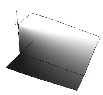
Figure 5: Graphs for Example 2: Steps and Deltas on {x=0}\{x=0\}.
Refer to caption
(a) Graph of non-negative solution φ\varphi where y↦φ⁡(0,y)y\mapsto\varphi(0,y) is a step.
Refer to caption
(b) Graph of non-negative solution ψ\psi where y↦ψ⁡(0,y)y\mapsto\psi(0,y) is a Dirac-δ\delta.

Setting f=φ⋅x−2f=\varphi\cdot{x}^{-2} and g=ψ⋅x−2g=\psi\cdot{x}^{-2}, we have non-negative functions on the half-plane that satisfy (72), but which are not C0​(H2¯)C^{0}(\overline{H^{2}}). In the case of ff, we have a solution with finite boundary values on x<0x<0 and infinite values on x≥0x\geq 0. In the case of gg, we have a solution with finite boundary values on x≠0x\neq 0, and g⁡(0,0)=∞g(0,0)=\infty.

Example 3. Solution that is a pulse on {x=0}\{x=0\}.

Solutions are translation-invariant in yy, so using translations of (143) we construct

φ⁡(x,y)=12​(y+1/2x2+(y+1/2)2−y−1/2x2+(y−1/2)2)\displaystyle\begin{aligned} &\varphi(x,y)\;=\;\frac{1}{2}\left(\frac{y+1/2}{\sqrt{x^{2}+(y+1/2)^{2}}}-\frac{y-1/2}{\sqrt{x^{2}+(y-1/2)^{2}}}\right)\\ \end{aligned} (144)

which solves φx​x−x−1​φx+φy​y=0\varphi_{xx}-x^{-1}\varphi_{x}+\varphi_{yy}=0. Restricted to the boundary {x=0}\{x=0\}, this is a unit pulse. The associated function f=φ⋅x−2=(x2+y2)−3/2f=\varphi\cdot{x}^{-2}=(x^{2}+y^{2})^{-3/2} solves fx​x+fy​y+3​x−1​fx=0f_{xx}+f_{yy}+3x^{-1}f_{x}=0.

Figure 6: Graphs for Example 3: A pulse, and a solution of (72) not determined by boundary values.
Refer to caption
(a) Graph of non-negative φ\varphi where y↦φ⁡(0,y)y\mapsto\varphi(0,y) is a pulse function.
Refer to caption
(b) Graph of non-negative, non-constant ff with finite and infinite values on the boundary.

Then ff has finite values on x∉[−12,12]x\notin[-\frac{1}{2},\frac{1}{2}]. If one considers, say, the quadrilateral Q={0<x<1}∩{−1<y<1}Q=\{0<x<1\}\cap\{-1<y<1\}, then we see that ff has finite values on ∂Q\partial{Q}, and so using the Fourier and Bessel series from (136) we can construct an L∞L^{\infty} solution f~\tilde{f} to the PDE that has f~=f\tilde{f}=f on ∂Q\partial{Q}. In particular, the function f−f~f-\tilde{f} is zero on ∂Q\partial{Q} but is non-constant.

This illustrates the necessity of the hypothesis of boundedness in Lemma 4.2.

Example 4. A solution that is only C1,α​(H2¯)∩C∞​(H2)C^{1,\alpha}(\overline{H^{2}})\cap{}C^{\infty}(H^{2}).

Consider the function

φ=y​x2+y2+x2​log⁡(y+x2+y2x),\displaystyle\varphi\;=\;{y}\sqrt{x^{2}+y^{2}}\,+\,{x^{2}}\log\left(\frac{y+\sqrt{x^{2}+y^{2}}}{x}\right), (145)

which solves φx​x+φy​y−x−1​φx=0\varphi_{xx}+\varphi_{yy}-x^{-1}\varphi_{x}=0. Note that φ∈C1,α​(H2¯)∩C∞​(H2)\varphi\in{}C^{1,\alpha}(\overline{H^{2}})\cap{C}^{\infty}(H^{2}) for all α∈[0,1)\alpha\in[0,1) but φ∉C1,1​(H2¯)\varphi\notin{}C^{1,1}(\overline{H^{2}}).

The fact that y↦φ⁡(0,y)y\mapsto\varphi(0,y) is piecewise quadratic rather than piecewise-linear provides an important counterpoint to the crucial assertion in Proposition 2.11 where piecewise linearity is asserted when the solution φ\varphi is a momentum function in a geometric situation.

Figure 7: Graph for Example 4: Piecewise quadratic growth at {x=0}\{x=0\}.
Refer to caption

This example shows the particular need for Propostion 2.11 where we show that the solutions that arise from our geometrical situations are in fact C2C^{2} up to the boundary, except at corners where they are Lipschitz.

Finally, this example show that although the PDE (71) has fundamental solutions (113) and has the ability to specify boundary values, but it is not hypoelliptic at the boundary {x=0}\{x=0\}. We have already seen that (72) is not hypoelliptic at the boundary.

5 The Quarter-Plane and General Polytopes

5.1 Polytope has one corner

First we consider the case that the polytope has just one corner. Take the example

φ1=a​y+b​x2+y2+α2​x2,φ2=c​y+d​x2+y2+β2​x2.\displaystyle\begin{aligned} \varphi^{1}&\;=\;ay\,+\,b\sqrt{x^{2}\,+\,y^{2}}\,+\,\frac{\alpha}{2}x^{2},\\ \varphi^{2}&\;=\;cy\,+\,d\sqrt{x^{2}\,+\,y^{2}}\,+\,\frac{\beta}{2}x^{2}.\end{aligned} (146)

Setting Φ=(φ1,φ2)T\Phi=(\varphi^{1},\varphi^{2})^{T} we have Jacobian and Jacobian determinant

D​Φ=(b​x​(x2+y2)−12+α​xa+b​y​(x2+y2)−12d​x​(x2+y2)−12+β​xc+d​y​(x2+y2)−12),det(D​Φ)=−x​(x2+y2)−12​((a​d−c​b)+(a​β−c​α)​(x2+y2)12+y⁡(b​β−α​d)).\displaystyle\begin{aligned} &D\Phi\;=\;\left(\begin{array}[]{ccc}bx\left(x^{2}+y^{2}\right)^{-\frac{1}{2}}+\alpha{}x&&a+by\left(x^{2}+y^{2}\right)^{-\frac{1}{2}}\\ dx\left(x^{2}+y^{2}\right)^{-\frac{1}{2}}+\beta{}x&&c+dy\left(x^{2}+y^{2}\right)^{-\frac{1}{2}}\end{array}\right),\\ &\det\left(D\Phi\right)\;=\;-x\left(x^{2}+y^{2}\right)^{-\frac{1}{2}}\left((ad-cb)+\left(a\beta-c\alpha\right)\left(x^{2}+y^{2}\right)^{\frac{1}{2}}+y\left(b\beta-\alpha{d}\right)\right).\end{aligned} (147)

It is impossible that det(D​Φ)\det(D\Phi) be zero away from {x=0}\{x=0\} or undefined away from (x,y)=(0,0)(x,y)=(0,0), or else d​φ1d\varphi^{1} and d​φ2d\varphi^{2} would be colinear which would imply the polytope has some additional edge or corner somewhere. Therefore r=x2+y2r=\sqrt{x^{2}+y^{2}} and yy must obey the linear inequalities

det(M)+det(N)​r+det(K)​y≠ 0,0≤|y|≤r\displaystyle\begin{aligned} &\det(M)\,+\,\det(N)r\,+\,\det(K)y\;\neq\;0,\quad\quad 0\leq|y|\leq{r}\end{aligned} (148)

where

M=(abcd),N=(aαcβ),K=(bαdβ).\displaystyle\begin{aligned} &M=\left(\begin{array}[]{cc}a&b\\ c&d\end{array}\right),\quad N=\left(\begin{array}[]{cc}a&\alpha\\ c&\beta\end{array}\right),\quad K=\left(\begin{array}[]{cc}b&\alpha\\ d&\beta\end{array}\right).\end{aligned} (149)

In order for (148) to hold, it is necessary and sufficient that |det(K)det(N)|≤1\left|\frac{\det(K)}{\det(N)}\right|\leq 1 and det(K)det(M)≥0\frac{\det(K)}{\det(M)}\geq 0 and det(M)≠0\det(M)\neq 0.

Lemma 5.1

Consider the map Φ:H2¯→ℝ2\Phi:\overline{H^{2}}\rightarrow\mathbb{R}^{2} where Φ=(φ1,φ2)T\Phi=(\varphi^{1},\varphi^{2})^{T}, and each φi\varphi^{i} satisfies (φi)x​x−x−1​(φi)x+(φi)y​y=0(\varphi^{i})_{xx}-x^{-1}(\varphi^{i})_{x}+(\varphi^{i})_{yy}=0. Assume Φ\Phi is C2C^{2} except at (0,0)(0,0), and that Φ\Phi is Lipschitz everywhere. Then either the image is either the half-plane and (possibly after G​L​(2,ℝ)GL(2,\mathbb{R}) recombination of φ1\varphi^{1}, φ2\varphi^{2}) we have

φ1=x2φ2=y\displaystyle\begin{aligned} &\varphi^{1}\;=\;x^{2}\\ &\varphi^{2}\;=\;y\end{aligned} (150)

or else (possibly after a G​L​(2,ℝ)GL(2,\mathbb{R}) recombination) the polytope is the first quadrant with

φ1=12​(−y+x2+y2)+α2​x2,φ2=12​(y+x2+y2)+β2​x2\displaystyle\begin{aligned} \varphi^{1}&\;=\;\frac{1}{\sqrt{2}}\left(-y\,+\,\sqrt{x^{2}\,+\,y^{2}}\right)\,+\,\frac{\alpha}{2}x^{2},\\ \varphi^{2}&\;=\;\frac{1}{\sqrt{2}}\left(y\,+\,\sqrt{x^{2}\,+\,y^{2}}\right)\,+\,\frac{\beta}{2}x^{2}\end{aligned} (151)

for some α\alpha, β\beta where α,β≥0\alpha,\beta\geq 0.

Proof. As indicated set Φ⁡(x,y)=(φ1​(x,y),φ2​(x,y))T\Phi(x,y)=(\varphi^{1}(x,y),\varphi^{2}(x,y))^{T}. At any smooth point on {x=0}\{x=0\}, the fact that (φi)x​x−x−1​(φi)x+(φi)y​y=0(\varphi^{i})_{xx}-x^{-1}(\varphi^{i})_{x}+(\varphi^{i})_{yy}=0 implies that (φi)x=0(\varphi^{i})_{x}=0 to first order. But then limx→0x−1​(φi)x=(φi)x​x\lim_{x\rightarrow 0}x^{-1}(\varphi^{i})_{x}=(\varphi^{i})_{xx}, so the first two terms cancel and we have (φi)y​y=0(\varphi^{i})_{yy}=0 at {x=0}\{x=0\}.

Therefore, away from (0,0)(0,0), the map y↦Φ⁡(0,y)y\mapsto\Phi(0,y) is actually linear. Including (0,0)(0,0), this map is piece-wise linear, and consists of two rays joined at one point 22 2 For an example of how this can fail if the “Lipschitz” hypothesis is removed, see Example 2. For an example of how this can fail if the “C2C^{2} except at (0,0)(0,0)” hypothesis is removed, see Example 4.. After possibly an affine recombination of φ1\varphi^{1}, φ2\varphi^{2}, we can therefore assume that y↦Φ⁡(0,y)y\mapsto\Phi(0,y) is the map y↦(12​(−y+|y|),12​(y+|y|))y\mapsto\left(\frac{1}{\sqrt{2}}\left(-y+|y|\right),\,\frac{1}{\sqrt{2}}\left(y+|y|\right)\right).

Consider the function ψ1=φ1−12​(−y+x2+y2)\psi^{1}=\varphi^{1}-\frac{1}{\sqrt{2}}\left(-y+\sqrt{x^{2}+y^{2}}\right). On {x=0}\{x=0\} we now have that ψ1​(0,y)=0\psi^{1}(0,y)=0. We wish to use Theorem 4.16, but we must show that ψ1≥0\psi^{1}\geq 0. First consider ψ~1=ψ1+x2\tilde{\psi}^{1}=\psi^{1}+x^{2}, which is still zero on {x=0}\{x=0\}. This may have negative components, but the negative part is within the wedge below the line y=1−xy=1-x (in fact, it is below the parabola y=12​(1−x2)y=\frac{1}{2}(1-x^{2}). The function ηϵ=−ϵ⁡(x4−4​(y−1)2​x2)\eta_{\epsilon}=-\epsilon(x^{4}-4(y-1)^{2}x^{2}) is zero on x=0x=0 and on y=1−12​xy=1-\frac{1}{2}x; therefore ηϵ<0\eta_{\epsilon}<0 on y=1−xy=1-x. Further, the growth of ηϵ\eta_{\epsilon} is quadratic, whereas the growth of the negative part ψ~−1\tilde{\psi}^{1}_{-} is linear.

Thus for any ϵ>0\epsilon>0 we have ηϵ<−ψ~−1\eta_{\epsilon}<-\tilde{\psi}^{1}_{-} for any ϵ\epsilon. Sending ϵ→0\epsilon\rightarrow 0, we see that ψ~−1=0\tilde{\psi}^{1}_{-}=0. Thus ψ~1≥0\tilde{\psi}^{1}\geq 0. Now we can use Theorem 4.16 to see there exists some α∈ℝ\alpha\in\mathbb{R} so that ψ~1​(x,y)=α~2​x2\tilde{\psi}^{1}(x,y)=\frac{\tilde{\alpha}}{2}x^{2} and therefore necessarily φ1​(x,y)=12​(−y+x2+y2)+α2​x2\varphi^{1}(x,y)=\frac{1}{\sqrt{2}}\left(-y+\sqrt{x^{2}+y^{2}}\right)+\frac{\alpha}{2}x^{2} for some constant α=α~−1\alpha=\tilde{\alpha}-1. Similarly we have φ2=12​(y+x2+y2)+β2​x2\varphi^{2}=\frac{1}{\sqrt{2}}\left(y+\sqrt{x^{2}+y^{2}}\right)+\frac{\beta}{2}x^{2}. The fact that we must have both α,β≥0\alpha,\beta\geq 0 follows simply from the considerations coming immediately after (149). □\Box

In [3] it was noticed that there is a 2-parameter family of metrics on any open polytope Σ2\Sigma^{2} without parallel lines that produces scalar flat metrics on (M4,J,ω)(M^{4},J,\omega). The next theorem shows that up to homothety these are precisely all metrics when the polytope has a single corner. This is the geometric version of Theorem 5.1.

Theorem 5.2 (cf. Theorem 1.7)

Assume (Σ,gΣ)(\Sigma,g_{\Sigma}) satisfies (A)-(F)—for instance it may be the reduction of some scalar flat (M4,J,ω,𝒳1,𝒳2)(M^{4},J,\omega,\mathcal{X}_{1},\mathcal{X}_{2})—and assume the associated metric polytope (Σ2,gΣ)(\Sigma^{2},g_{\Sigma}) is closed and has a single corner. Then (up to homothethy and S​L​(2,ℝ)SL(2,\mathbb{R}) re-combination) the momentum functions φ1\varphi^{1}, φ2\varphi^{2} necessarily have the form

φ1=12​(−y+x2+y2)+α2​x2,φ2=12​(y+x2+y2)+β2​x2\displaystyle\begin{aligned} \varphi^{1}&\;=\;\frac{1}{\sqrt{2}}\left(-y\,+\,\sqrt{x^{2}\,+\,y^{2}}\right)\,+\,\frac{\alpha}{2}x^{2},\\ \varphi^{2}&\;=\;\frac{1}{\sqrt{2}}\left(y\,+\,\sqrt{x^{2}\,+\,y^{2}}\right)\,+\,\frac{\beta}{2}x^{2}\end{aligned} (152)

where α,β≥0\alpha,\beta\geq 0. Therefore metric gΣg_{\Sigma} belongs precisely to a 2-parameter family of possibilities, parametrized by α\alpha and β\beta.

Proof. The “closure” assumption is that the polytope contains both of its rays: geometrically, neither ray can be “infinitely far away”. By Proposition 2.11, the potential functions φ1\varphi^{1}, φ2\varphi^{2}, when considered as functions of (x,y)(x,y) and as solutions to the PDE (71), are indeed C2C^{2} on edges and are Lipschitz everywhere. But Lemma 5.1 then implies φ1\varphi^{1}, φ2\varphi^{2} (after possible G​L​(2,ℝ)GL(2,\mathbb{R})-recombination) necessarily have the form given above. □\Box

Corollary 5.3

If the Kähler manifold (M4,J,ω,𝒳1,𝒳2)(M^{4},J,\omega,\mathcal{X}_{1},\mathcal{X}_{2}) is scalar-flat and has a closed polytope with a single corner, then the metric is necessarily in the 2-parameter family given by the momentum functions (152) and the recipe in §2.3.

Proof. Combine Theorem 5.2 with the description in §2.3. □\Box

5.2 Open polytopes with more than one corner

In the case where the polytope is unbounded but has more than two edges, the situation is a bit more complex. Homothetic G​L​(2,ℝ)GL(2,\mathbb{R}) transformations of φ1\varphi^{1}, φ2\varphi^{2} are able to stabilize precisely two vertices, but unlike the one-vertex case, the speed of parametrization of the two ray edges cannot also be fixed with such transformations.

Define the “outline” of the polytope to be the image of the map y↦(φ1​(0,y),φ2​(0,y))Ty\mapsto\left(\varphi^{1}(0,y),\varphi^{2}(0,y)\right)^{T}. In the case that the polytope contains all of its boundaries, then Proposition 2.11 asserts that this map is Lipschitz and piecewise linear. After fixing two vertices in place via G​L​(2,ℝ)GL(2,\mathbb{R})-transformation, the speed at which each linear segment is traversed is an independent variable. Therefore each of the NN edges contributes a degree of freedom to the space of polytope metrics. Two additional degrees of freedom express the possible addition of x2x^{2}-terms to each momentum function.

Theorem 5.4 (Generic Polytopes)

Assume (Σ2,gΣ)(\Sigma^{2},g_{\Sigma}) is a closed polytope that satisfies (A)-(F) and has n≥3n\geq 3 edges. Then the pair (φ1,φ2)(\varphi^{1},\varphi^{2}), as a function of (x,y)(x,y), belongs to an (n+2)(n+2)-parameter family of possibilities. As a result, the metric gΣg_{\Sigma} belongs to an (n+2)(n+2)-parameter family of possible polytope metrics.

Proof. The proof is to give a recipe for reconstructing the metric on the polytope from the behavior of (φ1,φ2)(\varphi^{1},\varphi^{2}) on the edges, and noting the degrees of freedom that appear. As noted above, the outline map y↦Φ⁡(0,y)=(φ1​(0,y)φ2​(0,y))y\mapsto\Phi(0,y)=\left(\begin{array}[]{c}\varphi^{1}(0,y)\\ \varphi^{2}(0,y)\end{array}\right) is Lipschitz and piecewise linear, so can be expressed as sums of terms of the form

Ψi​(y)=(αi​(y−yi)+βi​|y−yi|+ciγi​(y−y0)+δi​|y−y0|+di),Ψ⁡(0,y)=∑i=1n−1Ψi​(y).\displaystyle\Psi_{i}(y)=\left(\begin{array}[]{c}\alpha_{i}(y-y_{i})+\beta_{i}|y-y_{i}|+c_{i}\\ \gamma_{i}(y-y_{0})+\delta_{i}|y-y_{0}|+d_{i}\end{array}\right),\quad\Psi(0,y)=\sum_{i=1}^{n-1}\Psi_{i}(y).

Since yy is required to satisfy only d​y=−JΣ​d​xdy=-J_{\Sigma}{d}x, we may add a constant to yy to make sure that y1=0y_{1}=0. Given an outline (the image of y↦Φ⁡(0,y)y\mapsto\Phi(0,y)) along with the fact that the outline map is piecewise linear, the only freedom we have is choosing the speed of the parametrizations of each segment; this is nn degrees of freedom. With the first corner occurring at (φ1,φ2)=(0,1)(\varphi^{1},\varphi^{2})=(0,1) we have c1=0c_{1}=0, d1=1d_{1}=1, and from the speed of each segment, we can determine all of the rest of the constants.

Then we simply replace |y−yi||y-y_{i}| with x2+(y−yi)2\sqrt{x^{2}+(y-y_{i})^{2}} to obtain

Φ~i​(x,y)=(φ~i1​(x,y)φ~i2​(x,y))=(αi​(y−yi)+βi​x2+(y−yi)2+ciγi​(y−yi)+δi​x2+(y−yi)2+di).\displaystyle\widetilde{\Phi}_{i}(x,y)\;=\;\left(\begin{array}[]{cc}\widetilde{\varphi}_{i}^{1}(x,y)\\ \widetilde{\varphi}_{i}^{2}(x,y)\end{array}\right)\;=\;\left(\begin{array}[]{cc}\alpha_{i}(y-y_{i})\,+\,\beta_{i}\sqrt{x^{2}+(y-y_{i})^{2}}\,+\,c_{i}\\ \gamma_{i}(y-y_{i})\,+\,\delta_{i}\sqrt{x^{2}+(y-y_{i})^{2}}\,+\,d_{i}\\ \end{array}\right).

We have that each φ~i1\widetilde{\varphi}_{i}^{1}, φ~i2\widetilde{\varphi}_{i}^{2} satisfies the differential equation (71). Since ∑iΦ~i​(0,y)=Φ⁡(0,y)\sum_{i}\widetilde{\Phi}_{i}(0,y)=\Phi(0,y) by construction, by Theorem 4.16 there must be constants α\alpha, β\beta such that φ1​(x,y)=α2​∑iφi1\varphi^{1}(x,y)=\frac{\alpha}{2}\sum_{i}\varphi_{i}^{1} and φ2=β2+∑iφi2\varphi^{2}=\frac{\beta}{2}+\sum_{i}\varphi^{2}_{i}. Selection of α\alpha, β\beta give the final two degrees of freedom. □\Box

Corollary 5.5

If the scalar-flat Kähler manifold (M4,J,ω,𝒳1,𝒳2)(M^{4},J,\omega,\mathcal{X}_{1},\mathcal{X}_{2}) has a closed polytope with n≥3n\geq 3 edges, then the momentum map Φ=(φ1,φ2)T\Phi=(\varphi^{1},\varphi^{2})^{T} must be a member of an (n+2)(n+2)-parameter family of possibilities. Thus the metric gg on M4M^{4} lies within an (n+2)(n+2)-parameter family of possible scalar flat metrics.

Proof. Combine Theorem 5.4 with the description in §2.3. □\Box

Remark. To express Theorem 5.5 more intrinsically, note that if the polytope of (M4,J,ω,𝒳1,𝒳2)(M^{4},J,\omega,\mathcal{X}_{1},\mathcal{X}_{2}) has nn many edges, then b2​(M4)=n−2b_{2}(M^{4})=n-2. Thus if b2​(M4)>0b_{2}(M^{4})>0 then there are b2​(M4)+4b_{2}(M^{4})+4 degrees of freedom, up to homothety, in choosing scalar-flat metrics on complete Kähler 4-manifolds with two commuting holomorphic symmetries.

Remark. For the polytope of 3 edges (where b2​(M4)=1b_{2}(M^{4})=1), the recipe of Theorem 5.5 is carried out in Example 6 below.

Remark. Although we do not discuss the case that the polytope is not closed (that it has “edges” that are infinitely far away), it is not difficult to imagine how they could be built up, namely by adding together potentials of the form found in Example 2, along with the potentials used in this section. However we run into difficulties in the proof of uniqueness. The issue is that, after subtracting copies of such potentials, it is still possible that the resulting functions are not zero everywhere on the boundary. If one attempts to multiply such potentials φ\varphi by x−2x^{-2} to get f=x−2⋅φf=x^{-2}\cdot\varphi, there may be singularities on the boundary. Thus the analysis of Section 4 fails, as it relies on f∈C0​(H2¯)∩C∞​(H2)f\in{C}^{0}(\overline{H^{2}})\cap{C}^{\infty}(H^{2}).

5.3 Examples

Example 5. Construction of all doubly-invariant scalar-flat metrics on ℂ2\mathbb{C}^{2}.

These are precisely the Taub-NUTs, the achiral (or twisted) Taub-NUTs, and the flat metric. All of these are ALF metrics, except the flat metric which is ALE. According to our theorem, up to linear combinations of φ1\varphi^{1}, φ2\varphi^{2}, all quarter-plane examples have the form given in (151), and using (38) we have polytope metric

gΣ=1+α+β2​x2+y2+α−β2​yx2+y2​(d​x⊗d​x+d​y⊗d​y).\displaystyle\begin{aligned} &g_{\Sigma}\;=\;\frac{1\,+\,\frac{\alpha+\beta}{\sqrt{2}}\sqrt{x^{2}+y^{2}}+\frac{\alpha-\beta}{\sqrt{2}}y}{\sqrt{x^{2}+y^{2}}}\,\left(dx\otimes{d}x+dy\otimes{d}y\right).\end{aligned} (161)

Setting M=α+β2M=\frac{\alpha+\beta}{\sqrt{2}} and k=α−βα+βk=\frac{\alpha-\beta}{\alpha+\beta} (so we are free to choose any M>0M>0 and any k∈[−1,1]k\in[-1,1]) and changing to polar coordinates, we have

gΣ=1+M​r​(1+k​sin⁡θ)r(dr2+r2dθ2),0≤θ≤π2,KΣ=−M​1−M​k​r​(k+sin⁡θ)(1+M​r​(1+k​sin⁡θ))3.\displaystyle\begin{aligned} &g_{\Sigma}\;=\;\frac{1+Mr\left(1+k\sin\theta\right)}{r}\,\left(dr^{2}\,+\,r^{2}d\theta^{2}\right),\quad 0\leq\theta\leq\frac{\pi}{2},\\ &K_{\Sigma}\;=\;-M\frac{1\,-\,Mk\,r\left(k+\sin\theta\right)}{\left(1+Mr\left(1+k\sin\theta\right)\right)^{3}}.\end{aligned} (162)

When k=0k=0, these are the Taub-NUT metrics. Also using (38), we can write down the metric in (φ1,φ2)(\varphi^{1},\varphi^{2})-coordinates, which allows us to easily write down the metric on M4M^{4} as well. However for generic α,β>0\alpha,\beta>0, the epression for G=x⁡(d​e​t​(A))​A​ATG=x(det(A))AA^{T} is rather complex.

Example 6. Construction of all doubly-invariant scalar-flat metrics on T​ℂ​P1T\mathbb{C}P^{1}.

These include the Eguchi-Hanson metric. These metrics are represented by polytopes with three edges: two rays and an adjoining segment. Under G​L​(2,ℝ)GL(2,\mathbb{R}) recombinations of φ1,φ2\varphi^{1},\varphi^{2}, this polytope is the standard polytope with vertices at (0,1)(0,1) and (1,0)(1,0).

Figure 8: Plot for Example 6: Polytope outline for toric metrics on T​ℂ​P2T\mathbb{C}P^{2}, with direction of parametrization indicated.
Refer to caption

We have five remaining degrees of freedom: three degrees for the speed of each edge, and two degrees of freedom arising from the possible addition of x2x^{2} terms to φ1\varphi^{1}, φ2\varphi^{2}. Thus up to homothety all such metrics are given by

φ1=v22​2​(y+x2+y2)+(v32−v22​2)​((y−2v2)+x2+(y−2v2)2)+α2​x2φ2=1+v12​(−y+x2+y2)−v22​2​(y+x2+y2)+v22​2​((y−2v2)+x2+(y−2v2)2)+β2​x2\displaystyle\begin{aligned} \varphi^{1}&=\frac{v_{2}}{2\sqrt{2}}\left(y+\sqrt{x^{2}+y^{2}}\right)+\left(\frac{v_{3}}{2}-\frac{v_{2}}{2\sqrt{2}}\right)\left(\left(y-\frac{\sqrt{2}}{v_{2}}\right)+\sqrt{x^{2}+\left(y-\frac{\sqrt{2}}{v_{2}}\right)^{2}}\right)+\frac{\alpha}{2}x^{2}\\ \varphi^{2}&=1+\frac{v_{1}}{2}\left(-y+\sqrt{x^{2}+y^{2}}\right)-\frac{v_{2}}{2\sqrt{2}}\left(y+\sqrt{x^{2}+y^{2}}\right)\\ &\quad\quad+\frac{v_{2}}{2\sqrt{2}}\left(\left(y-\frac{\sqrt{2}}{v_{2}}\right)+\sqrt{x^{2}+\left(y-\frac{\sqrt{2}}{v_{2}}\right)^{2}}\right)+\frac{\beta}{2}x^{2}\end{aligned} (163)

The numbers v1,v2,v3>0v_{1},v_{2},v_{3}>0 encode the speeds at which y↦Φ⁡(0,y)y\mapsto\Phi(0,y) maps onto the three linear pieces of the outline. We remark that there are certainly other choices of parametrization.

Example 7. A polytope with an “edge at infinity.”

We begin with the 4-manifold M4=𝕊2×ℍ2M^{4}=\mathbb{S}^{2}\times\mathbb{H}^{2}, where ℍ2\mathbb{H}^{2} is the pseudosphere:

g=d​r1⊗d​r1+sin2⁡(r1)​d​θ1⊗d​θ1+d​r2⊗d​r2+e2​r2​d​θ2⊗d​θ2.\displaystyle g\;=\;dr^{1}\otimes{}dr^{1}+\sin^{2}(r^{1})d\theta^{1}\otimes{d}\theta^{1}\,+\,dr^{2}\otimes{}dr^{2}+e^{2r^{2}}d\theta^{2}\otimes{}d\theta^{2}. (164)

The moment functions are φ1=−cos⁡(r1)\varphi^{1}=-\cos(r^{1}) and φ2=er2\varphi^{2}=e^{r^{2}}. Because r1∈[0,π]{r}^{1}\in[0,\pi] and r2∈(−∞,∞)r^{2}\in(-\infty,\infty), we have that the range of (φ1,φ2)(\varphi^{1},\varphi^{2}) is precisely [0,1]×(0,∞)[0,1]\times(0,\infty).

Figure 9: Plots for Example 7: A polytope with an “edge at infinity.”
Refer to caption
(a) The dashed segment is not part of the image of the moment map, and is infinitely far away as measured in gΣg_{\Sigma}.
Refer to caption
(b) Graph of V=x\sqrt{V}=x as a function of φ1\varphi^{1}, φ2\varphi^{2}.

We have the metrics

g=11−(φ1)2​(d​φ1)2+(1−(φ1)2)​(d​θ1)2+1(φ2)2​(d​φ2)2+(φ2)2​(d​θ2)2,gΣ=11−(φ1)2​(d​φ1)2+1(φ2)2​(d​φ2)2\displaystyle\begin{aligned} g&\;=\;\frac{1}{1-\left(\varphi^{1}\right)^{2}}\left(d\varphi^{1}\right)^{2}\,+\,\left(1-\left(\varphi^{1}\right)^{2}\right)\left(d\theta^{1}\right)^{2}+\frac{1}{\left(\varphi^{2}\right)^{2}}\left(d\varphi^{2}\right)^{2}\,+\,\left(\varphi^{2}\right)^{2}\left(d\theta^{2}\right)^{2},\\ g_{\Sigma}&\;=\;\frac{1}{1-\left(\varphi^{1}\right)^{2}}\left(d\varphi^{1}\right)^{2}+\frac{1}{\left(\varphi^{2}\right)^{2}}\left(d\varphi^{2}\right)^{2}\end{aligned} (165)

This produces

x=𝒱=|∇φ1|​|∇φ2|=1−(φ1)2⋅φ2,andy=φ1​φ2,φ1=yx2+y2,andφ2=x2+y2.\displaystyle\begin{aligned} &x\;=\;\sqrt{\mathcal{V}}=|\nabla\varphi^{1}||\nabla\varphi^{2}|=\sqrt{1-\left(\varphi^{1}\right)^{2}}\cdot\varphi^{2},\quad{\rm and}\quad y\;=\;\varphi^{1}\varphi^{2},\\ &\varphi^{1}\;=\;\frac{y}{x^{2}+y^{2}},\quad{\rm and}\quad\varphi^{2}\;=\;\sqrt{x^{2}+y^{2}}.\end{aligned} (166)

Figure 5(a) in Example 2 is actually the graph of φ1\varphi^{1} as a function of xx, yy.

Example 8. A Polytope with a disconnected outline.

This also furnishes an example of a polytope Σ2\Sigma^{2} so that x=𝒱x=\sqrt{\mathcal{V}} with yy gives a complex function z=x+−1​yz=x+\sqrt{-1}y with a critical point, so zz is not one-to-one; see Proposition 2.8.

Using the scalar flat metric on 𝕊2×ℍ2\mathbb{S}^{2}\times\mathbb{H}^{2}, where this time the hyperbolic piece has a “two-ended trumpet” metric, we have

g=d​r1⊗d​r1+sin2⁡(r1)​d​θ1⊗d​θ1+d​r2⊗d​r2+cosh2⁡(r2)​d​θ2⊗d​θ2.\displaystyle g\;=\;dr^{1}\otimes{}dr^{1}+\sin^{2}(r^{1})d\theta^{1}\otimes{d}\theta^{1}\,+\,dr^{2}\otimes{}dr^{2}+\cosh^{2}(r^{2})d\theta^{2}\otimes{}d\theta^{2}. (167)

This gives φ1=−cos⁡(r1)\varphi^{1}=-\cos(r^{1}) and φ2=sinh⁡(r2)\varphi^{2}=\sinh(r^{2}), with range Σ2=[−1,1]×ℝ\Sigma^{2}=[-1,1]\times\mathbb{R}. The polytope metric

g=11−(φ1)2​d​φ1⊗d​φ1+11+(φ2)2​d​φ2⊗d​φ2\displaystyle g\;=\;\frac{1}{1-\left(\varphi^{1}\right)^{2}}\,d\varphi^{1}\otimes{d}\varphi^{1}\,+\,\frac{1}{1+\left(\varphi^{2}\right)^{2}}\,d\varphi^{2}\otimes{d}\varphi^{2} (168)

and we have

x=(1−(φ1)2)​(1+(φ2)2),y=φ1φ2,φ1=12​1−(x2+y2)+(1−(x2+y2)2)2+ 4​y2φ2=12​−1+(x2+y2)+(1−(x2+y2)2)2+ 4​y2\displaystyle\begin{aligned} &x\;=\;\sqrt{\left(1-\left(\varphi^{1}\right)^{2}\right)\left(1+\left(\varphi^{2}\right)^{2}\right)},\quad y\;=\;\varphi^{1}\varphi^{2},\\ &\varphi^{1}\;=\;\frac{1}{\sqrt{2}}\sqrt{1-\left(x^{2}+y^{2}\right)+\sqrt{\left(1-\left(x^{2}+y^{2}\right)^{2}\right)^{2}\,+\,4y^{2}}}\\ &\varphi^{2}\;=\;\frac{1}{\sqrt{2}}\sqrt{-1+\left(x^{2}+y^{2}\right)+\sqrt{\left(1-\left(x^{2}+y^{2}\right)^{2}\right)^{2}\,+\,4y^{2}}}\end{aligned} (169)
Figure 10: Plots for Example 8: A polytope with disconnected outline.
Refer to caption
(a) The polytope is the strip −1≤φ1≤1-1\leq\varphi^{1}\leq 1.
Refer to caption
(b) Graph of x=𝒱x=\sqrt{\mathcal{V}} as a function of φ1\varphi^{1}, φ2\varphi^{2}.

Clearly xx and therefore z=x+−1​yz=x+\sqrt{-1}y have a critical point. This compliments Proposition 2.8, as the polytope has disconnected edges.

References

  • [1] M. Abreu, Kähler geometry of toric varieties and extremal metrics, International Journal of Mathematics, 9 (1998) 641–651
  • [2] M. Abreu, Kähler geometry of toric manifolds in symplectic coordinates, Portugaliae Mathematica 67, No. 2 (2010) 121–153
  • [3] M. Abreu and R. Sena-Dias, Scalar-flat Kähler metrics on non-compact symplectic toric 4-manifolds, Annals of Global Analysis and Geometry, 41 No. 2 (2012) 209–239
  • [4] V. Arnold, Mathematical Methods of Classical Mechanics, Graduate Texts in Mathematics, 60, Springer-Verlag, New York, 1978
  • [5] M. Atiyah, Convexity and commuting Hamiltonians, Bulletin of the London Mathematical Society, 14 (1982) 1–15
  • [6] D. Calderbank, L. David, and P. Gauduchon, The Guillemin formula and Kähler metrics on toric symplectic manifolds, Journal of Symplectic Geometry 4, no. 1 (2002) 767–784
  • [7] D. Calderbank and H. Pedersen, Self-dual Einstein metrics with torus symmetry, Journal of Differential Geometry, 60 (2002) 485–521
  • [8] D. Calderbank and M. Singer, Einstein metrics and complex singularities, Inventiones Mathematicae, 156 (2004) 405–443
  • [9] S.Y. Cheng and S.T. Yau, Differential equations on Riemannian manifolds and their geometric applications, Communication on Pure and Applied Mathematics, 28 (1975) 333–354
  • [10] P. Daskalopoulos and R. Hamilton, Regularity of the free boundary for the porous medium equation, Journal of the American Mathematical Society, 9 (1998) 899–965
  • [11] T. Delzant, Hamiltoniens périodique et images convexes de l’application moment, Bulletin de la Société Mathématique de France, 116 (1988) 315–339 F
  • [12] S. Donaldson, A generalized Joyce construction for a family of nonlinear partial differential equations, Journal of Gökova Geometry/Topology Conferences, 3 (2009)
  • [13] S. Donaldson, Constant scalar curvature metrics on toric surfaces, Geometric and Functional Analysis, 19 No. 1 (2009) 83–136
  • [14] C. Epstein and R. Mazzeo, Degenerate Diffusion Operators Arising in Population Biology, Annals of Mathematical Studies, Princeton University Press, Princeton, NJ, 2013
  • [15] P. Feehan, A classical Perron method for existence of smooth solutions to boundary value and obstacle problems for degenerate-elliptic operators via holomorphic maps, arXiv:1302.1849
  • [16] P. Feehan and C. Pop, Degenerate-elliptic operators in mathematical finance and higher-order regularity for solutions to variational equations, Advances in Differential Equations, 20 No. 3/4 (2015) 361–432
  • [17] P. Feehan and C. Pop, A Schauder approach to degenerate-parabolic partial differential equations with unbounded coefficients, arXiv:1112.4824
  • [18] D. Gilbarg and N.S. Trudinger, Elliptic partial differential equations of second order, 2nd Ed., Springer-Verlag, New York, 1983.
  • [19] A. Grigor’yan and J. Masamune, Parabolicity and stochastic completeness of manifolds in terms of the Green formula, Journal de Mathématiques Pures et Appliquées 9 (2013) 607–632
  • [20] V. Guillemin, Kähler structures on toric varieties, Journal of Differential Geometry, 40 (1994) 285–309
  • [21] V. Guillemin and S. Sternberg, Convexity properties of the moment mapping, Inventiones Mathematicae, 67 (1982) 491–513
  • [22] S. Heston, A closed-form solution for options with stochastic volatility with applications to bond and currency options, Review of Financial Studies, 6 (1989) 12–45
  • [23] I. Holopainen and P. Koskela, Volume growth and parabolicity, Proceedings of the American Mathematical Society, 129 No. 11 (2001) 3425–3435
  • [24] N. Honda and J. Viaclovsky, Toric LeBrun metrics and Joyce metrics, Geometry and Topology, 17 No 5 (2013) 2923–2934
  • [25] L. Hormander, Hypoelliptic second order differential equations, Acta Mathematica, 119 No 1 (1967) 147–171
  • [26] J.J. Kohn and L. Nirenberg, Degenerate elliptic-parabolic equations of second order, Communications in Pure and Applied Mathematics, 20 (1967) 797–872
  • [27] D. Joyce, Explicit construction of self-dual 4-manifolds, Duke Mathematics Journal, 77 (1995) 519–552
  • [28] Y. Karshon and E. Lerman, Non-compact symplectic toric manifolds, arXiv.org/abs/0907.2891
  • [29] C. LeBrun, Conter-examples to the generalized positive action conjecture, Communications in Mathematical Physics, 118 (1988) 591–596
  • [30] E. Lerman and S. Tolman, Hamiltonian torus actions on symplectic orbifolds and toric varieties, Transactions of the American Mathematical Society, 349 (1997) 4201–4230
  • [31] P. Li, On the structure of complete Kähler manifolds with nonnegative curvature near infinity, Inventiones Mathematicae, 99 (1990) 576–600
  • [32] P. Li and L. Tam, Positive harmonic functions on complete manifolds with non-negative curvature outside a compact set, Annals of Mathematics, 125 (1987) 171–207
  • [33] P. Li and L. Tam, Harmonic functions and the structure of complete manifolds, Journal of Differential Geometry, 35 (1992) 359–383
  • [34] P. Li and L. Tam, Green’s functions, harmonic functions, and volume comparison, Journal of Differential Geometry, 41 (1995) 277–318
  • [35] R. Sena-Dias, Curvature of scalar-flat Kähler metrics on non-compact symplectic toric 4-manifolds, Differential Geometry and its Applications, 33 (2014) 149– 182
  • [36] R. Schoen and S.T. Yau, Lectures on Differential Geometry, International Press (1994).
  • [37] B. Weber, First betti number of Kähler manifolds with weakly pseudoconvex boundary ArXiv:1110.4571