Maximally persistent cycles in random geometric complexesThanks: O.B. gratefully acknowledges the support NSF DMS-1418261 and NSF DMS-1209155.Thanks: M.K. gratefully acknowledges support from DARPA #N66001-12-1-4226, NSF #CCF-1017182, NSF #DMS-1352386, the Institute for Mathematics and its Applications, and the Alfred P. Sloan FoundationThanks: P.S. was funded by the EU project TOPOSYS (FP7-ICT-318493-STREP)

The study of topological properties of random graphs has a long history, dating back to classical results on the connectivity, cycles, and largest components in Erdős–Renyi graphs [30, 31]. Generalizations have been developed in several directions. One direction is to consider different models of random graphs (see, e.g. [13, 45]). Another direction is to consider higher-dimensional topological properties, resulting in the study of random simplicial complexes rather than random graphs, where in addition to vertices and edges the structure consists also of triangles, tetrahedra and higher dimensional simplexes (see, e.g. [4, 38, 40, 42]). The study of random simplicial complexes focuses mainly on their homology, which is a natural generalization of the notions of connected components and cycles in graphs. Homology is an algebraic topology framework that is used to study cycles in various dimensions, where (loosely speaking) a $k$-dimensional cycle can be thought of as the boundary of a $k+1$ dimensional solid (see Section 2 for more details).

In random geometric simplicial complexes, the vertices are generated by a random point process (e.g. Poisson) in a metric space, and then geometric conditions are applied to determine which of the simplexes should be included in the complex. The two most studied models are the random Čech and Vietoris-Rips complexes (see Section 2 for definitions). Several recent papers have studied various aspects of the topology of these complexes (see [7, 10, 12, 39, 41, 51, 52] and the survey [9]). These papers contain theorems which characterize the phase transitions where homology appears and disappears, estimates for the Betti numbers (the number of $k$-dimensional cycles), limiting distributions, etc. While this line of research presents a deep and interesting theory, it is also motivated by data analysis applications.

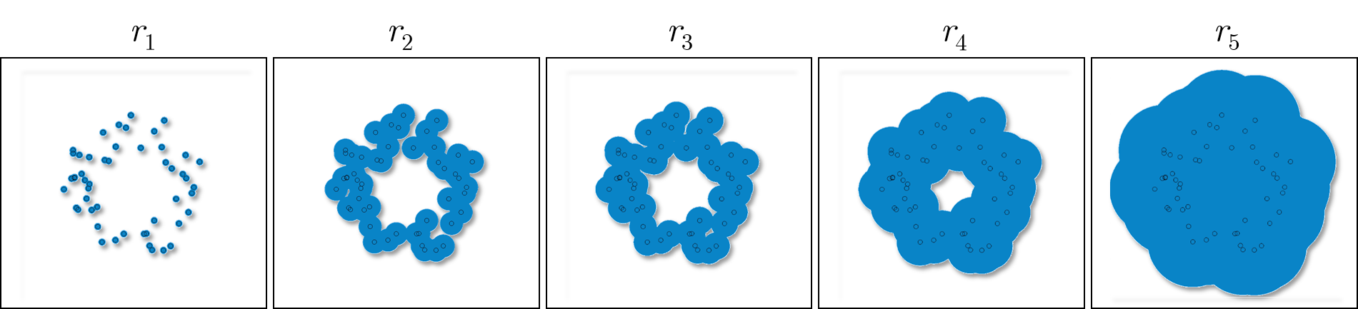
Topological data analysis (TDA) is a recently emerging field that focuses on extracting topological features from sampled data, and uses them as an input for various data analytic and statistical algorithms. The main idea behind it is that topological properties could help us understand the structure underlying the data, and provide us with a set of features that are robust to various types of deformations (cf. [17, 18, 34]). Geometric complexes play a key role in computing topological features from a finite set of data points. The construction of these complexes usually depends on one or more parameters (e.g. radius of balls drawn around the sample points), and the ability to properly extract topological features depends on choosing this parameter correctly. One of the most powerful tools in TDA is a multi-scale version of homology, called persistent homology (see Section 2), which was developed mainly to solve this problem of sensitive parameter tuning. In persistent homology, instead of finding the best parameter values, one considers the entire range of possible values. As the parameter values change, the observed topological features change (e.g. cycles are created and filled in). Persistent homology tracks these changes and provides a way to measure the significance of the features that show up in this process. One way to represent the information provided by persistent homology is via barcodes, see Figure 2. Here, every bar corresponds to a feature in the data and its endpoints correspond to the times (parameter value) where the feature was created and terminated. The underlying philosophy in TDA is that topological features that survive (or persist) through a long range of parameter values are significant and related to real topological structures in the data (or the “topological signal”), whereas ones with a shorter lifespan are artifacts of the finite sampling, and correspond to noise (see [32]). This approach motivates the following question: How long does a “long range” of parameters (or a long bar in the barcode) have to be in order to be considered significant? Phrased differently - how long should we expect this range to be, if the sample points were entirely random, without any underlying structure or features? This is the main question we try to answer in this paper.

To be more specific, in this paper we study the case where the data points are generated by a homogeneous Poisson process in the unit $d$-dimensional cube $[0,1]^{d}$ ($d>1$) with intensity $n$, denoted by $\mathcal{P}_{n}$. We consider the persistent homology of both the Čech complex $\mathcal{C}(\mathcal{P}_{n},r)$ and the Rips complex $\mathcal{R}(\mathcal{P}_{n},r)$, where the scale parameter $r$ is the radius of the balls used to create these complexes (see Section 2). We denote by $\Pi_{k}(n)$ the maximal persistence of a cycle in the degree $k$ persistent homology ($1\leq k\leq d-1$) of either the Čech or the Rips complex. Note that $\Pi_{k}(n)$ is a property of the persistent homology, where we consider all possible radii, and therefore it does not depend $r$. Our main result shows that, with high probability,

in the sense that $\Pi_{k}(n)$ can be bounded from above and below by a matching term up to a constant factor. The precise definitions and statements are presented in Section 3. The proofs for the upper and lower bounds require very different techniques. To prove the upper bound we present a novel ‘isoperimetric-type’ statement (Lemma 4.1) that links the persistence of a cycle to the number of vertices that are used to form it. The lower bound proof uses an exhaustive search for a specific construction that guarantees the creation of a persistent cycle.

In addition to proving the theoretical result, in Section 7 we also present extensive numerical experiments confirming the computed bounds and empirically computing the implied constants. These results also suggest a conjectural law of large numbers. Finally, we note that while the results in this paper are presented for the homogeneous Poisson process on a $d$-dimensional cube, they should hold with minor adjustments also to non-homogenous processes as well as for shapes other than the cube. We also predict that our statements will hold for more generic point processes (e.g. weakly sub-Poisson processes), using some of the statements made in [51]. The detailed analysis of these more generic cases is left as future work.

Earlier work: The study of the topology of random geometric complexes has been growing rapidly in the past decade. Most of the results so far are related to homology rather than persistent homology (i.e. fixing the parameter value). The study in [12, 39] focuses mainly on the phase transitions for appearance and vanishing of homology, which can be viewed as higher dimensional generalizations of the phase transition for connectivity in random graphs. In [7, 10, 41, 52] more emphasis was given to the distribution of the Betti numbers, namely the number of cycles that appear. Similar questions for more general point processes have also been considered in [51]. In [2, 44] simplicial complexes generated by distributions with an unbounded support were studied from an extreme value theory perspective. The recent survey [9] overviews recent progress in this area.

The study of random persistent homology, on the other hand, is at its very initial stages. Recall that the $0$-th homology represent the connected components in a space. Thus, the results in [3, 46] about the connectivity threshold in random geometric graphs could be viewed as related to the $0$-th persistence homology of either the Čech or the Rips complex. The first study of persistent homology in degree $k\geq 1$ for a random setting was for $n$ points chosen uniformly i.i.d. on a circle by Bubenik and Kim [15]. In this setting, they used the theory of order statistics to describe the limiting distribution of the persistence diagram. Another direction of study is the persistence diagrams of random functions. In [8], the authors study the “persistent Euler characteristic” of Gaussian random fields.

Another line of research (see e.g. [11, 20, 21, 22, 23, 24, 32]) focuses on statistical inference using persistent homology, and include results about confidence intervals, consistency and robustness for topological estimation, subsampling and bootstrapping methods, and more.

Finally, we point out the earlier work in geometric probability [5], measuring the largest convex hole for a set of random points in a convex planar region $R$. A convex hole is generated when there is a subset of points for which the convex hull is empty (i.e. contains no other points from the set). The size of a convex hole is then measured combinatorially, as the number of vertices generating the hole. In [5] it is shown that the largest hole has $\Theta\left(\log n/\log\log n\right)$ vertices, regardless of the shape of the ambient convex region $R$. In this paper we are also measuring the size of the largest hole, but in a very different sense. We are using the algebraic-topological notion of holes (via persistent homology), rather than combinatorial notion of counting vertices, so as far as we can tell the fact that these two ways of measuring the size of the largest hole have the same right of growth (when $d=2$ and $k=1$) is something of a coincidence.

As far as we know, this article presents the first detailed probabilistic analysis for persistent $k$th homology of random geometric complexes, for $k\geq 1$.

The structure of the paper is as follows. In Section 2 we provide the topological and probabilistic building blocks we will use throughout the paper. In Section 3 we present the main result - the asymptotic behavior of maximally persistent cycles. In Sections 4 and 5 we provide the main parts of the proof for the random Čech complex (upper and lower bounds, respectively). Some parts of the proofs require more knowledge in algebraic topology than the others, and we present those in Section 6 (including the proof for the Rips complex). Finally, in Section 7 we present simulation results, complementing the main (asymptotic) result of the paper.

In this section we provide a brief introduction to the topological and probabilistic notions used in this paper.

For the remainder of this paper assume that $d\geq 2$ and $1\leq k\leq d-1$ are fixed. Let $\mathcal{P}_{n}$ be the Poisson process defined above, and define

Let $\PH_{k}(n)$ be the $k$-th persistent homology of either of the filtrations for $\mathcal{U},\mathcal{C},\textrm{ or }\mathcal{R}$ (it will be clear from the context which filtration we are looking at). Note that from the Nerve Lemma (2.3) we have that $\mathcal{U}(n,r)\simeq\mathcal{C}(n,r)$, so we will state the results only for $\mathcal{C}$ and $\mathcal{R}$. However, some of the statements we make are easier to prove for the balls in $\mathcal{U}$ rather than the simplexes in $\mathcal{C}$, and we shall do so.

For every cycle $\gamma\in\PH_{k}(n)$ we denote by $\gamma_{birth},\gamma_{death}$ the birth and death times (radii) of $\gamma$, respectively. Commonly (see [17, 34]), the persistence of a cycle is measured by the length of the corresponding bar in the barcode, namely by the difference $\delta(\gamma):=\gamma_{death}-\gamma_{birth}$. In this paper, however, we choose to define the persistence of $\gamma$ in a multiplicative way as

There are several reasons for defining the persistence of a cycle this way.

• •

  This definition is equivalent to saying that we measure the difference in a logarithmic scale. Studying persistent homology in the logarithmic scale is common [24, 16, 37, 47, 49].

• •

  This definition is scale invariant, which is desirable, since ‘topological significance’ should focus on shape rather than size. For example, consider the cycles corresponding to $\gamma_{1},\gamma_{2}$ in Figure 3. These two cycles are created by exactly the same configuration of points, just at a different scale. Therefore, we would like to say that these cycles are equally significant. Clearly, $\delta(\gamma_{1})>\delta(\gamma_{2})$, while $\pi(\gamma_{1})=\pi(\gamma_{2})$. Thus, our definition works better in this case.

  In addition, this scale invariance guarantees that a linear change in the units used to measure the data (e.g. from inches to cm, or from degrees Celsius to Fahrenheit) will not affect the persistence value.

• •

  One purpose of using a persistence measure is to differentiate between cycles that capture phenomena underlying the data, and those who are created merely due to chance. To this end, the ‘physical size’ of the cycle is not necessarily the correct measure. Consider, for example, the cycles corresponding to $\gamma_{2}$ and $\gamma_{3}$ in Figure 3. Intuitively, we would like to claim that $\gamma_{2}$ is more significant than $\gamma_{3}$, as the former is created by a very ‘stable’ configuration of points, while the latter is created by outliers that clearly tell us nothing about the underlying structure. In this example, taking the ‘additive’ persistence we will have that $\delta(\gamma_{2})<\delta(\gamma_{3})$, simply because the overall size of the annulus is much smaller than that of the triangle. However, taking multiplicative persistence yields $\pi(\gamma_{2})>\pi(\gamma_{3})$, which is more consistent with our intuition.

• •

  Both the Čech and Vietoris–Rips complexes are important in TDA, and the natural relationship between these complexes is a multiplicative one (see (2.2)). Because of this relationship, our results hold for both random Čech and Rips complexes, up to a constant factor (see Section 6.3). Indeed, the majority of approximation results for geometric complexes are multiplicative [48, 19, 27], making multiplicative persistence more relevant to existing stability guarantees.

• •

  The argument from Section 5 of this paper suggests that there are many cycles $\gamma$ for which $\gamma_{birth}=o(\gamma_{death})$. In this case, it is hard to differentiate between cycles by looking at $\gamma_{death}-\gamma_{birth}\approx\gamma_{death}$.

Our main interest is in the maximal persistence over all $k$-cycles, defined as

More specifically, we are interested in the asymptotic behavior of $\Pi_{k}(n)$ as $n\to\infty$. The main result in this paper is that $\Pi_{k}(n)$ scales like the function $\Delta_{k}(n)$, defined by

In particular we have the following theorem.

Remarks:

1. (1)

   The constants $A_{k}$ and $B_{k}$ depend on $k$ (the homology degree), $d$ (the ambient dimension), and on whether we consider the Čech or the Rips complex. We conjecture that a law of large numbers holds, namely that $\Pi_{k}(n)/\Delta_{k}(n)\to C_{k}$ for some $A_{k}\leq C_{k}\leq B_{k}$. For some evidence for this conjecture, see the experimental results in Section 7. In the following sections we will prove Theorem 3.1.

2. (2)

   The additive persistence $\delta(\gamma)$ can be bounded naively by the result on the contractibility of the Čech complex in [39]. More concretely, Theorem 6.1 states that if $r\geq c\left(\frac{\log n}{n}\right)^{1/d}$ then the Čech complex is contractible (w.h.p.). This implies that for every cycle $\gamma$ we have $\delta(\gamma)\leq\gamma_{\mathrm{death}}\leq c\left(\frac{\log n}{n}\right)^{1/d}$. Similar statements can be made about $\PH_{0}$ using the connectivity radius in [3, 46] (which is of the same $(\log n/n)^{1/d}$ scale). However, these are only crude upper bounds on the additive persistence, that do not differentiate between the different cycles in persistent homology, or even between different degrees of homology (note that these bounds do not depend on $k$).

3. (3)

   The study in [39] suggests the following upper bound for $\Pi_{k}(n)$. As mentioned before, we know that $\gamma_{\mathrm{death}}\leq c\left(\frac{\log n}{n}\right)^{1/d}$ for all $\gamma$. In addition, the analysis in [39] shows that if $n^{k+1}r^{dk}\to 0$ then $H_{k}(\mathcal{C}(n,r))=0$, which implies that $\gamma_{\mathrm{birth}}\geq c^{\prime}n^{-\frac{k+2}{d(k+1)}}$ for some $c^{\prime}>0$. Therefore, we have that $\pi(\gamma)=O\left({(\log n)^{1/d}n^{\frac{1}{d(k+1)}}}\right)$. However, as we shall see later, this is a very crude upper bound.

For this section and the next one, consider the Čech complex only. We want to prove the upper bound in Theorem 3.1. That is, we need to show that there exists a constant $B_{k}>0$ depending only on $k$ and $d$, so that with high probability

The main idea in proving the upper bound in Theorem 3.1 is to show that large cycles require the formation of a large connected component in $\mathcal{C}(n,r)$ at a very early stage (small radius $r$). To this end we will provide two bounds: (1) a lower bound for the size of the connected component supporting a large cycle (Lemma 4.1), and (2) an upper bound for the size of connected components in $\mathcal{C}(n,r)$ for small values of $r$ (Lemma 4.2).

The proof for this lemma requires more working knowledge in algebraic topology than the rest of this paper, and we defer it to Section 6. At this point, we would like to suggest an intuitive explanation. Suppose that $\mathcal{C}(n,r)$ contains a $k$-cycle such that all the points generating it lie on a $k$-dimensional sphere of radius $R$, and such that there are no points of $\mathcal{P}_{n}$ inside the sphere. In that case the death time of the cycle will be $R$ and then $\pi(\gamma)=p\geq R/r$. The minimum number of balls of radius $r$ required to cover a $k$-dimensional sphere of radius $R$ is known as the “covering number” and is proportional to $(R/r)^{k}=p^{k}$. The cycle created is then a part of a connected component of $\mathcal{C}(n,r)$ containing at least $C\times p^{k}$ vertices. Intuitively, creating a cycle with the same birth and death times in any other way (i.e. not necessarily around a sphere) will require coverage of an area larger than the $k$-dimensional sphere, and therefore larger connected components. To make this statement precise, in Section 6 we present an isoperimetric-type inequality for $k$-cycles. Note that this statement is completely deterministic (i.e. non-random).

The following lemma bounds the number of vertices in a connected component of the Čech complex $\mathcal{C}(n,r)$, for small values of $r$.

With these two lemmas, we can prove the upper bound in Theorem 3.1.

In this section we prove the lower bound part of Theorem 3.1 for the Čech complex $\mathcal{C}(n,r)$, namely that there exists $A_{k}>0$ (depending on $k$ and $d$), such that with high probability,

In other words, we need to show that with a high probability there exists $\gamma\in\PH_{k}(n)$ with $\pi(\gamma)\geq A_{k}\Delta_{k}(n)$.

To show that, we take the unit cube $Q=[0,1]^{d}$ and divide it into small cubes of side $2L$. The number of small cubes we can fit in $Q$ denoted by $M$ satisfies $M\geq C_{3}L^{-d}$ for some $C_{3}>0$. Denoting the small cubes by $Q_{1},\ldots,Q_{M}$, we want to show that at least one of these cubes contains a large cycle. Let $Q_{i}$ be one of these cubes, and think of it as centered at the origin, so that $Q_{i}=[-L,L]^{d}$. Let $\ell<L/4$, denote $\hat{L}=\left\lfloor{L/\ell}\right\rfloor\times\ell$, and define

In other words, $S_{i}$ is a “thickened” version of the boundary of a $k+1$ dimensional cube of side $\hat{L}\approx L$ (see Figure 4).

We will show that if the balls of radius $r$ around $\mathcal{P}_{n}$ cover $S_{i}$ but leave most of $Q_{i}$ empty then $\mathcal{C}(n,r)$ would have a $k$-dimensional cycle. Choosing $L$ and $\ell$ properly we can make sure that this cycle has the desirable persistence. More specifically, take $S_{i}$ and split it into $m$ cubes of side $\ell$, denoted by $S_{i,1},S_{i,2},\ldots,S_{i,m}$ (see Figure 4). The number of boxes $m$ is almost proportional to the ratio of the volumes of $S_{i}$ and the $S_{i,j}$-s, and therefore $m\leq C_{4}(L/\ell)^{k}$ for some $C_{4}>0$. The following lemma uses the process $\mathcal{P}_{n}$ but is in fact non-random, and provides a lower-bound to the persistence of the cycles we are looking for.

The proof of this lemma also requires some working knowledge in algebraic topology, and therefore we postpone it to Section 6. Intuitively, the assumptions of the lemma guarantee that for every $r\in[r_{1},r_{2}]$, where $r_{1}=\sqrt{d}\ell$ and $r_{2}=L/4$, the union of balls $\mathcal{U}(\mathcal{P}_{n}\cap Q_{i},r)$ covers $S_{i}$, and is disconnected from the rest of the balls. Therefore, its shape is “similar” to $S_{i}$ and forms a nontrivial $k$-cycle. Since this cycle exists through the entire range $[r_{1},r_{2}]$ its persistence is greater than $r_{2}/r_{1}=L/4\sqrt{d}\ell$.

Following Lemma 5.1, we define the event

then $E=E_{1}\cup E_{2}\cup\cdots\cup E_{M}$ is the event that at least one of the $Q_{i}$ cubes contains a large cycle. Lemma 5.1 suggests that to prove there exists a large cycle it is enough to show that $E$ occurs with high probability. We start by bounding the probability of the complement event. The next lemma shows that given the right choice of $L=L(n)$ and $\ell=\ell(n)$ we can guarantee that $E=E^{(n)}$ satisifes $\mathbb{P}\left(E\right)\to 1$.

As mentioned above, the proofs for Lemmas 4.1 and 5.1 require some working knowledge in algebraic topology. In particular, we will be making use of the definitions of chains, cycles, boundaries and induced maps in both simplicial and singular homology. For more background, see [36] or [43]. To make reading the paper fluent for readers who are less familiar with the subject, we deferred these proofs to this section. Also included in this section is the translation of Theorem 3.1 from the Čech to the Rips complex.

References

- [1] Random number generation in c++11. https://isocpp.org/files/papers/n3551.pdf.
- [2] Robert J. Adler, Omer Bobrowski, and Shmuel Weinberger. Crackle: The homology of noise. Discrete Comput. Geom., pages 1–25, 2014. arXiv:1301.1466.
- [3] Martin JB Appel and Ralph P. Russo. The connectivity of a graph on uniform points on . Statistics & Probability Letters, 60(4):351–357, 2002.
- [4] Lior Aronshtam and Nathan Linial. When does the top homology of a random simplicial complex vanish? Random Structures & Algorithms, 46(1):26–35, 2015.
- [5] József Balogh, Hernán González-Aguilar, and Gelasio Salazar. Large convex holes in random point sets. Comput. Geom., 46(6):725–733, 2013.
- [6] Ulrich Bauer, Michael Kerber, and Jan Reininghaus. PHAT (Persistent Homology Algorithm Toolbox), 2014. [Online; accessed 7-May-2015].
- [7] Omer Bobrowski and Robert J. Adler. Distance functions, critical points, and the topology of random čech complexes. Homology, Homotopy and Applications, 16(2):311–344, 2014.
- [8] Omer Bobrowski and Matthew Strom Borman. Euler integration of Gaussian random fields and persistent homology. J. Topol. Anal., 4(1):49–70, 2012.
- [9] Omer Bobrowski and Matthew Kahle. Topology of random geometric complexes: a survey. To appear in: Topology in Statistical Inference, the Proceedings of Symposia in Applied Mathematics, 2014.
- [10] Omer Bobrowski and Sayan Mukherjee. The topology of probability distributions on manifolds. Probability Theory and Related Fields, 161(3-4):651–686, 2014.
- [11] Omer Bobrowski, Sayan Mukherjee, and Jonathan Taylor. Topological consistency via kernel estimation. arXiv preprint arXiv:1407.5272, 2014.
- [12] Omer Bobrowski and Shmuel Weinberger. On the vanishing of homology in random Čech complexes. arXiv preprint arXiv:1507.06945, 2015.
- [13] Béla Bollobás and Oliver M Riordan. Mathematical results on scale-free random graphs. Handbook of graphs and networks: from the genome to the internet, pages 1–34, 2003.
- [14] Karol Borsuk. On the imbedding of systems of compacta in simplicial complexes. Fund. Math., 35:217–234, 1948.
- [15] Peter Bubenik and Peter T. Kim. A statistical approach to persistent homology. Homology, Homotopy Appl., 9(2):337–362, 2007.
- [16] Mickaël Buchet, Frédéric Chazal, Steve Oudot, and Donald R. Sheehy. Efficient and robust persistent homology for measures. In Proceedings of the 26th ACM-SIAM symposium on Discrete algorithms. SIAM. SIAM, 2015.
- [17] Gunnar Carlsson. Topology and data. Bull. Amer. Math. Soc. (N.S.), 46(2):255–308, 2009.
- [18] Gunnar Carlsson, Tigran Ishkhanov, Vin De Silva, and Afra Zomorodian. On the local behavior of spaces of natural images. International journal of computer vision, 76(1):1–12, 2008.
- [19] Frédéric Chazal, Vin De Silva, and Steve Oudot. Persistence stability for geometric complexes. Geometriae Dedicata, 173(1):193–214, 2014.
- [20] Frédéric Chazal, Brittany Terese Fasy, Fabrizio Lecci, Alessandro Rinaldo, Aarti Singh, and Larry Wasserman. On the bootstrap for persistence diagrams and landscapes. arXiv preprint arXiv:1311.0376, 2013.
- [21] Frédéric Chazal, Brittany Terese Fasy, Fabrizio Lecci, Alessandro Rinaldo, and Larry A. Wasserman. Stochastic convergence of persistence landscapes and silhouettes. In 30th Annual Symposium on Computational Geometry, SOCG’14, Kyoto, Japan, June 08 - 11, 2014, page 474, 2014.
- [22] Frédéric Chazal, Marc Glisse, Catherine Labruère, and Bertrand Michel. Convergence rates for persistence diagram estimation in topological data analysis. In Proceedings of the 31th International Conference on Machine Learning, ICML 2014, Beijing, China, 21-26 June 2014, pages 163–171, 2014.
- [23] Frédéric Chazal, Leonidas J Guibas, Steve Y Oudot, and Primoz Skraba. Scalar field analysis over point cloud data. Discrete & Computational Geometry, 46(4):743–775, 2011.
- [24] Frédéric Chazal, Leonidas J Guibas, Steve Y Oudot, and Primoz Skraba. Persistence-based clustering in riemannian manifolds. Journal of the ACM (JACM), 60(6):41, 2013.
- [25] Kenneth L Clarkson. Nearest-neighbor searching and metric space dimensions. Nearest-neighbor methods for learning and vision: theory and practice, pages 15–59, 2006.
- [26] Vin de Silva and Robert Ghrist. Coverage in sensor networks via persistent homology. Algebr. Geom. Topol., 7:339–358, 2007.
- [27] Tamal K Dey, Fengtao Fan, and Yusu Wang. Graph induced complex on point data. Computational Geometry, 48(8):575–588, 2015.
- [28] H. Edelsbrunner. The union of balls and its dual shape. Discrete and Computational Geometry, 13(1):415–440, 1995.
- [29] Herbert Edelsbrunner. The union of balls and its dual shape. In Proceedings of the ninth annual symposium on Computational geometry, pages 218–231. ACM, 1993.
- [30] Paul Erdős and Alfréd Rényi. On random graphs. I. Publ. Math. Debrecen, 6:290–297, 1959.
- [31] Paul Erdős and Alfréd Rényi. On the evolution of random graphs. Bull. Inst. Internat. Statist, 38(4):343–347, 1961.
- [32] Brittany Terese Fasy, Fabrizio Lecci, Alessandro Rinaldo, Larry Wasserman, Sivaraman Balakrishnan, and Aarti Singh. Confidence sets for persistence diagrams. Ann. Statist., 42(6):2301–2339, 2014.
- [33] Herbert Federer and Wendell H. Fleming. Normal and integral currents. Ann. of Math. (2), 72:458–520, 1960.
- [34] Robert Ghrist. Barcodes: the persistent topology of data. Bull. Amer. Math. Soc. (N.S.), 45(1):61–75, 2008.
- [35] Larry Guth. Notes on Gromov’s systolic estimate. Geom. Dedicata, 123:113–129, 2006.
- [36] Allen Hatcher. Algebraic topology. Cambridge University Press, Cambridge, 2002.
- [37] Benoit Hudson, Gary L. Miller, Steve Y. Oudot, and Donald R. Sheehy. Mesh enhanced persistent homology. 2009.
- [38] Matthew Kahle. Topology of random clique complexes. Discrete Math., 309(6):1658–1671, 2009.
- [39] Matthew Kahle. Random geometric complexes. Discrete Comput. Geom., 45(3):553–573, 2011.
- [40] Matthew Kahle. Sharp vanishing thresholds for cohomology of random flag complexes. Ann. of Math. (2), 179(3):1085–1107, 2014.
- [41] Matthew Kahle and Elizabeth Meckes. Limit theorems for Betti numbers of random simplicial complexes. Homology Homotopy Appl., 15(1):343–374, 2013.
- [42] Nathan Linial and Roy Meshulam. Homological connectivity of random 2-complexes. Combinatorica, 26(4):475–487, 2006.
- [43] James R. Munkres. Elements of algebraic topology. Addison-Wesley Publishing Company, Menlo Park, CA, 1984.
- [44] Takashi Owada and Robert J Adler. Limit theorems for point processes under geometric constraints (and topological crackle). arXiv preprint arXiv:1503.08416, 2015.
- [45] Mathew Penrose. Random geometric graphs, volume 5 of Oxford Studies in Probability. Oxford University Press, Oxford, 2003.
- [46] Mathew D. Penrose. The longest edge of the random minimal spanning tree. The Annals of Applied Probability, pages 340–361, 1997.
- [47] Jeff M. Phillips, Bei Wang, and Yan Zheng. Geometric Inference on Kernel Density Estimates. arXiv:1307.7760 [cs], July 2013. arXiv: 1307.7760.
- [48] Donald R Sheehy. Linear-size approximations to the vietoris–rips filtration. Discrete & Computational Geometry, 49(4):778–796, 2013.
- [49] Donald R. Sheehy. The persistent homology of distance functions under random projection. In Proceedings of the thirtieth annual symposium on Computational geometry, page 328. ACM, 2014.
- [50] The CGAL Project. CGAL User and Reference Manual. CGAL Editorial Board, 4.6 edition, 2015.
- [51] D. Yogeshwaran, Robert J. Adler, and others. On the topology of random complexes built over stationary point processes. The Annals of Applied Probability, 25(6):3338–3380, 2015.
- [52] D. Yogeshwaran, Eliran Subag, and Robert J. Adler. Random geometric complexes in the thermodynamic regime. submitted, arXiv:1403.1164, 2014.
- [53] Afra Zomorodian and Gunnar Carlsson. Computing persistent homology. Discrete & Computational Geometry, 33(2):249–274, 2005.