Numerical Methods for the Inverse Nonlinear Fourier Transform
Abstract
We introduce a new numerical method for the computation of the inverse nonlinear Fourier transform and compare its computational complexity and accuracy to those of other methods available in the literature. For a given accuracy, the proposed method requires the lowest number of operations.
Index Terms:
Nonlinear Fourier transform, inverse scattering transform, nonlinear Schrödinger equation, optical fiber communication.I Introduction
The propagation of light in optical fibers is governed by the nonlinear Schrödinger equation (NLSE), which accounts for the interplay of dispersion and nonlinearity. In the lossless case, the NLSE admits an analytical solution based on the inverse scattering transform (also known as nonlinear Fourier transform—NFT) [1]. On this basis, during the ’80s and the ’90s, research on soliton transmission in optical fibers was carried out extensively. However, despite a great effort, soliton systems never caught on commercially and were eventually abandoned in favor of simpler and more effective transmission techniques originally developed for linear channels. Recently, an alternative approach to communication over nonlinear channels—originally proposed in [2] and further generalized in [3] and [4]—is gaining new attention from the optical fiber community. Rather than using solitons as information carriers, the idea is that of encoding information onto the discrete and/or continuous spectrum of the Zakharov-Shabat operator (the scattering data), which evolves trivially and linearly along the fiber, such that the encoded information can be easily and accurately recovered from the optical signal after propagation at any distance, without any impact from dispersion and nonlinearity. This approach requires the computation of the inverse NFT at the transmitter to obtain the transmitted time-domain signal from the modulated scattering data, and the computation of the direct NFT at the receiver to extract the scattering data from the received time-domain signal. Both operations are, in general, quite involved and research on efficient numerical methods for their implementation is in progress [5, 6, 4, 7, 8, 9].
In this work, we focus on the numerical computation of the inverse NFT. We consider two methods available in the literature [5, 4] and propose an alternative method based on iterated convolutions evaluated through the fast Fourier transform (FFT) algorithm. All the methods are tested for the focusing NLSE in the soliton-free case (i.e., when only the continuous spectrum of the Zakharov-Shabat operator is present), which is of particular interest for information transmission based on nonlinear inverse synthesis [4]. Finally, we investigate and compare the accuracy and computational complexity of all the methods.
II Numerical methods
We consider the focusing NLSE in the normalized form
| (1) |
We assume to know the scattering data at a given distance and we focus on the inverse scattering problem (or inverse NFT) to obtain the corresponding NLSE solution .11 1 Hereafter, the dependence on is inessential and will be omitted. This problem leads to the Gel’fand-Levitan-Marchenko equation (GLME) [10]
| (2) |
where the integral kernel is a function of the scattering data. Specifically, considering the soliton-free case, where is the reflection coefficient. The solution of the NLSE is finally obtained as .
Let for and otherwise. The GLME can be rewritten in the form of the Marchenko integral equations
| (3) |
and the NLSE solution obtained as . In the following we assume to know on a uniform grid in the interval with step and we analyze three different numerical methods to solve the system (3), in order to find the solution of (1) for . Specifically, we consider the uniform grid on given by for with discretization step . The complexity of the methods is measured by considering the required number of complex products, assuming that the FFT of a vector of elements requires complex products.
An efficient numerical way to compute the inverse NFT, assuming , and therefore , is presented in [4]. The authors, using the Nyström method with a rectangular quadrature scheme to approximate the integrals in (3), find the solution by solving a linear system characterized by a Toeplitz matrix of size . The method of Trench for the inversion of non-Hermitian Toeplitz matrices [11] is used to recursively compute the solution for every value . For this reason, let us name this method Nyström-Trench (NT). The resulting algorithm computes the solution in the desired interval with complexity22 2 The computational complexity of the methods presented in [4] and [5] is not indicated by the authors. The values reported here refer to the most efficient implementations that we were able to devise.
| (4) |
However, due to the recursive nature of the algorithm, the complexity remains almost unchanged if the solution is computed in a lower number of points .
Another technique to solve system (3) with for , (i.e., in points in the interval ) is presented in [5], where the Nyström method with composite Simpson’s quadrature rule is considered. For a fixed time , the resulting linear system is solved by means of the conjugate gradient method. Therefore, we refer to this scheme as the Nyström conjugate gradient (NCG) method. Since we deal only with diagonal and upper-left triangular Hankel matrices, the complexity of the method can be reduced by using the FFT algorithm to compute the matrix-vector products required by the conjugate gradient method. As a result, the number of operations required to compute the solution in the desired interval is2
| (5) |
where is the number of iterations of the conjugate gradient method, which is assumed to be the same for every for the sake of simplicity. In this case, the solution is independently evaluated at each time in the given interval, such that depends significantly on the number of points .
Now, let us define a new iterative method to solve the system (3) for with discretization step . The main idea is that, by defining the auxiliary functions for and otherwise, with , the integrals in (3) can be seen as convolutions between these functions and the kernel and efficiently computed by means of the FFT algorithm. Therefore, considering a proper starting value for and iteratively updating the values of and by alternately computing the integrals in (3), we define an iterative method that, under certain conditions on and , converges to the solution of the system. As a starting point for at , we pick the solution found at the previous point , as we are dealing with continuous functions. The resulting algorithm is
where denotes convolution, is the th estimate of the function , and the corresponding auxiliary function. We refer to this method as the iterative convolution (IC) method. The number of operations required to find the solution in the points inside the interval is
| (12) |
Also in this case, depends significantly on the number of points and can be reduced by evaluating the solution with a larger step size.
III Numerical results
With the purpose of comparing the methods presented above, we consider the single-pulse signal considered in [4]
| (13) |
where . In this case, the scattering data are known and the GLME kernel is [4]
| (14) |
for and . We consider the interval and show the results only for , as similar results are obtained for different values of the parameters.
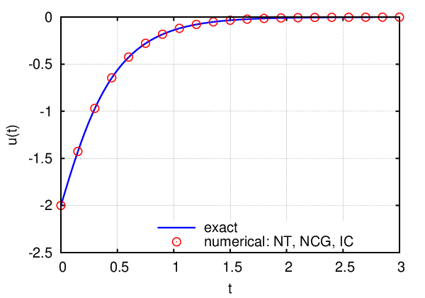
In Fig. 1 we compare the analytical solution (13) with the numerical results obtained with and . At this scale, all the numerical results are practically superimposed (and are, therefore, represented by a single curve to avoid cluttering the figure) and equal the exact solution. Since the new IC method is an iterative method, whose starting point at depends on the previous solution found at , it is interesting to investigate its convergence properties when the solution is evaluated with a different resolution (keeping unchanged the resolution for the evaluation of the integrals). Fig. 2 shows the modulus of the error, i.e., the difference between (13) and the numerical approximation, as a function of for , different iteration numbers , and different resolutions .
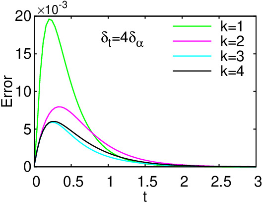
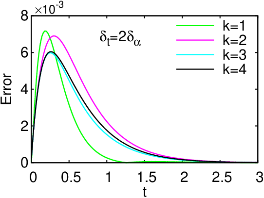
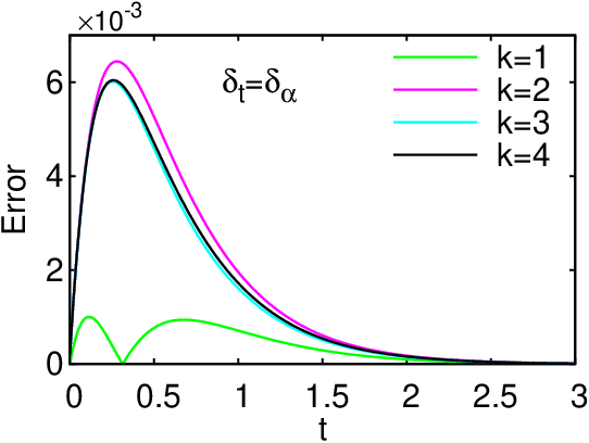
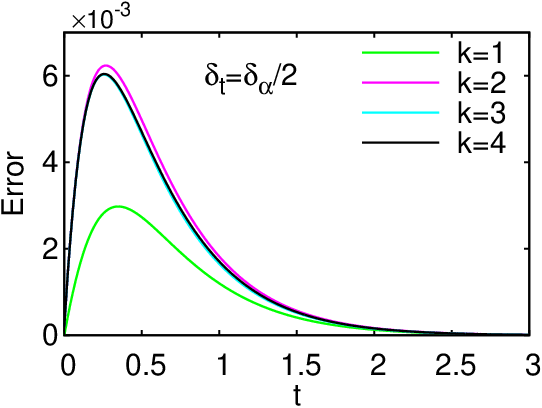
In all the cases, three iterations are enough to reach the convergence. However, in the case , the error after the first iteration is significantly lower than the error obtained after the convergence is reached. This quite surprising result has been observed also for different resolutions and for different pulse shapes (not shown here due to a lack of space). However, we have not been able to find a good explanation for this behavior, which is still under investigation. Given its particular properties, in the rest of the paper we will refer to the IC method with and as the IC1 method.
Fig. 3 compares the convergence properties of the IC method (for ) to those of the NCG method (for and any , as they are independent of ), showing how the root-mean-square error (RMSE) evaluated over the whole interval evolves with the number of iterations.
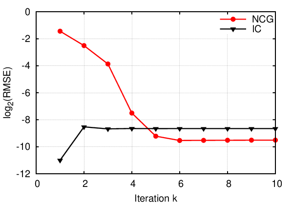
Thanks to the composite Simpson’s quadrature rule employed by the NCG method (which is more accurate than the rectangular quadrature rule implicitly employed by the IC method when using the FFT to compute the convolutions), the final RMSE reached by the NCG method is lower than the RMSE reached by the IC method. However, the IC method converges faster (after 3 iterations) than the NCG method (after 6 iterations). The same fast convergence of the IC method is observed also for higher values of (as shown in Fig. 2). However, in the special case , as observed before, the IC method achieves an even lower RMSE at the first iteration (IC1 method). Such a fast convergence is obtained thanks to the good starting value for indicated in (II). A convergence of the iterative method is observed in all the considered cases. This is, however, not guaranteed in general, as the convergence depends on specific conditions on and that are currently being investigated.
For all the methods, both the accuracy and the complexity depend on the resolution employed for the quadrature rules. Fig. 4 shows the RMSE as a function of for all the considered methods.
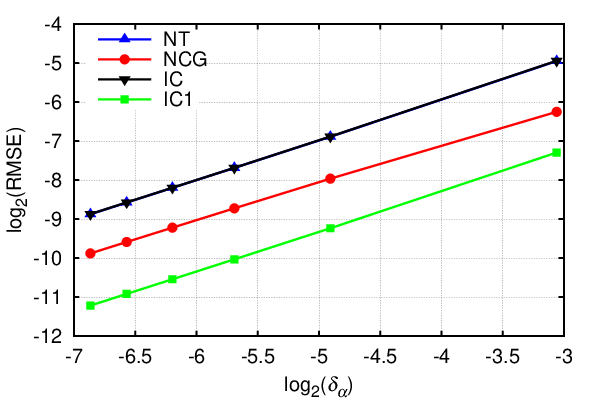
In the NT and IC1 methods, the resolution is set to and by construction, respectively. On the other hand, in the NCG and IC methods, can be selected as an integer multiple of without affecting the accuracy. The RMSE values obtained with the NT and IC methods are practically the same, as they are both based on a rectangular quadrature rule for the computation of the integrals in (3). The NCG method, thanks to the more accurate composite Simpson’s quadrature rule, achieves a lower RMSE for the same resolution . Finally, the IC1 method achieves an even lower RMSE.
Fig. 4 can be used to determine, for each method, what is the resolution (and, correspondingly, the number of points ) required for the computation of the integrals in order to find the solution with a given accuracy. This, in turn, will affect the complexity of the method according to (4), (5), or (12). Another relevant parameter that affects the computational complexity of the NCG and IC methods (but not that of the NT and IC1 methods) is the resolution with which the solution is needed (or, equivalently, the number of points in which the solution must be computed). Fig. 5 compares the computational complexity required by the various methods, computed according to (4), (5), and (12), to obtain the solution with a desired RMSE of (about in Fig. 4), as a function of the desired resolution .
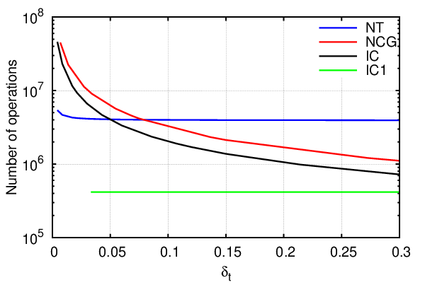
According to Fig. 4, the required resolution is for the NT and IC methods, for the NCG method, and for the IC1 method. The number of iterations required to reach the convergence is for the NCG method and for the IC method. By construction, the minimum resolution is for the NT, NCG, and IC methods, and for the IC1 method. However, if desired, the resolution can be increased by computing the solution in a lower number of points in the given interval . This will significantly reduce the computational complexity of the NCG and IC methods, but will leave the complexity of the NT and IC1 methods almost unaffected.33 3 Even if the solution is needed in a lower number of points , the NT and IC1 algorithms must be anyway executed for points. In the NT case, however, some operations can be saved, slightly reducing the computational complexity with respect to what is reported in (4). For any resolution , the NCG and IC methods have a similar complexity. In particular, the latter is slightly more convenient, though the former could be probably improved by using a more accurate quadrature rule or employing preconditioning. Both methods are more complex than the NT method when employed at full resolution, but become less complex when the solution is required in a lower number of points (the IC method for and the NCG method for ). Finally, the IC1 method is significantly less complex than the NT method (by about one order of magnitude) and less complex than the NCG and IC methods even at high resolutions . However, the behavior of the IC1 method is still under investigation and its superior performance, though observed also in other cases (not reported in this paper for a lack of space), has not been fully explained nor demonstrated for a generic signal.
IV Conclusions
A new numerical method for the computation of the inverse nonlinear Fourier transform has been proposed. The solution is obtained after iterated convolutions with the GLME kernel, which are efficiently computed trough the FFT algorithm. The accuracy and computational complexity of the proposed method have been investigated and compared to those of two other methods available in the literature, both exploiting the Nyström method in combination with either the conjugate gradient algorithm [5] or the Trench algorithm [4]. The obtained results show that, for a desired accuracy, the proposed method requires the lowest number of operations. The relation between the discretization step with which the integrals of the GLME are approximated and the time resolution with which the solution is computed (which need not be the same) is also discussed for all the methods, and the dependence of accuracy and complexity on those two parameters is investigated. When the two parameters are equal, the proposed method shows a very good but peculiar behavior which is still under investigation. Further investigation is also required to compare the algorithms in different scenarios, such as for the defocusing NLSE or in the presence of discrete eigenvalues in the nonlinear spectrum of the signal.
Acknowledgment
This work was supported in part by the Italian MIUR under the FIRB project COTONE
References
- [1] V. E. Zakharov and A. B. Shabat, “Exact theory of two-dimensional self-focusing and one-dimensional self-modulation of waves in nonlinear media,” Sov. Phys.-JETP, vol. 34, pp. 62–69, 1972.
- [2] A. Hasegawa and T. Nyu, “Eigenvalue communication,” J. Lightwave Technol., vol. 11, no. 3, pp. 395–399, Mar. 1993.
- [3] M. I. Yousefi and F. R. Kschischang, “Information transmission using the nonlinear Fourier transform, Part III: Spectrum modulation,” IEEE Trans. Inf. Theory, vol. 60, no. 7, pp. 4346–4369, Jul. 2014.
- [4] S. T. Le, J. E. Prilepsky, and S. K. Turitsyn, “Nonlinear inverse synthesis for high spectral efficiency transmission in optical fibers,” Optics express, vol. 22, no. 22, pp. 26 720–26 741, 2014.
- [5] A. Aricò, G. Rodriguez, and S. Seatzu, “Numerical solution of the nonlinear Schrödinger equation, starting from the scattering data,” Calcolo, vol. 48, no. 1, pp. 75–88, 2011.
- [6] M. I. Yousefi and F. R. Kschischang, “Information transmission using the nonlinear Fourier transform, Part II: Numerical methods,” IEEE Trans. Inf. Theory, vol. 60, no. 7, pp. 4329–4345, Jul. 2014.
- [7] S. Wahls and H. V. Poor, “Fast numerical nonlinear Fourier transforms,” arXiv preprint arXiv:1402.1605, 2014.
- [8] L. Fermo, C. van der Mee, and S. Seatzu, “Scattering data computation for the Zakharov-Shabat system,” arXiv preprint arXiv:1502.04628, 2015.
- [9] S. Wahls and H. V. Poor, “Fast inverse nonlinear Fourier transform for generating multi-solitons in optical fiber,” arXiv preprint arXiv:1501.06279, 2015.
- [10] M. J. Ablowitz and H. Segur, Solitons and the inverse scattering transform. SIAM, 1981, vol. 4.
- [11] S. Zohar, “Toeplitz matrix inversion: The algorithm of W. F. Trench,” Journal of the ACM (JACM), vol. 16, no. 4, pp. 592–601, 1969.