Bayesian optimal design for ordinary differential equation models with application in biological science
Abstract
Bayesian optimal design is considered for experiments where the response distribution depends on the solution to a system of non-linear ordinary differential equations. The motivation is an experiment to estimate parameters in the equations governing the transport of amino acids through cell membranes in human placentas. Decision-theoretic Bayesian design of experiments for such nonlinear models is conceptually very attractive, allowing the formal incorporation of prior knowledge to overcome the parameter dependence of frequentist design and being less reliant on asymptotic approximations. However, the necessary approximation and maximization of the, typically analytically intractable, expected utility results in a computationally challenging problem. These issues are further exacerbated if the solution to the differential equations is not available in closed-form. This paper proposes a new combination of a probabilistic solution to the equations embedded within a Monte Carlo approximation to the expected utility with cyclic descent of a smooth approximation to find the optimal design. A novel precomputation algorithm reduces the computational burden, making the search for an optimal design feasible for bigger problems. The methods are demonstrated by finding new designs for a number of common models derived from differential equations, and by providing optimal designs for the placenta experiment.
Keywords: Approximate coordinate exchange algorithm; decision-theoretic design; Gaussian process emulation; nonlinear design.
Introduction
The dynamics behind a complex physical process can often be described by a set of non-linear ordinary differential equations, where the solution to these equations represents the evolution of system states with respect to time. It is common for the system of equations to depend on some unknown physical properties (parameters) of the process in question and, potentially, on some additional controllable variables. In this paper, new methods are presented for designing experiments for the estimation of statistical models built on the solution to such a system of equations; that is, choosing the most informative combinations of time points and values of the controllable (design) variables at which observations of the physical process should be made. A decision-theoretic approach is adopted, and hence the quality of a design is measured via the expectation of a utility function chosen to encapsulate the aims of the experiment.
We assume equations with system states modeled as a function of time and design variables with values held in the treatment vector . The -vector holds the physical parameters requiring estimation. For notational simplicity, the dependence of the system states on and is usually suppressed, with , unless multiple treatments or parameter vectors are being considered. We mostly find designs for initial value problems, with defined via equations
| (1) |
where is the gradient vector of with respect to time , denotes initial conditions and, for given , is a continuous function satisfying the Lipschitz condition (see Iserles, 2009, p. 3). This latter assumption ensures equation (1) has a unique solution.
Our research is motivated by experiments to study the transport of serine, an amino acid, within a human placenta. Specifically, interest is in the movement of serine across a placental cell membrane (called a vesicle). In the experiments, initial amounts (l) of both radioactive and non-radioactive serine are placed exterior and interior to the vesicle, and then the amount of radioactive serine interior to the vesicle is measured at a series of time points. The experimenters have control over initial amounts of both the interior and exterior non-radioactive serine for each experiment, and the times (in seconds) at which observations are taken. The theoretical interior amounts of radioactive and non-radioactive serine at time form the system states, , with the design variables, , being, respectively, the exterior amounts of radioactive and non-radioactive serine at time . The equations governing the evolution of the system states are
| (2) |
where
, , and initial conditions are the amounts of radioactive and non-radioactive serine interior to the vesicle at time . Here, the four physical parameters correspond to the maximum uptake (), the proportion of the reaction occurring through active transport () and two reaction rates ( and ). The values of these parameters are of scientific interest. See Panitchob et al. (2015) and Widdows et al. (2017) for further details of the model and experiment.
To model experimental data from a physical process governed by (1), we build a statistical model linking the physical parameters to noisy observations of the system states, or functions thereof, via an assumed data-generating process dependent on the solution to the equations (see, for example, Ramsay et al. 2007). We also assume that an experiment can be conducted where these observations are collected at various different times and, possibly, from multiple runs of the experiment with different combinations of values of the design variables. Let denote the number of runs in the experiment, with the th run being made for treatment and initial conditions , with observations being made at time points (). At each time point, observations are taken on different responses. Let be the -vector of observations from the th run, and be the vector of observations from the whole experiment.
We describe the experimental data using statistical model
| (3) |
with a specified probability distribution, a -vector of nuisance parameters, and a vector specifying the design, chosen from the space of possible designs . The dependence of (3) on physical parameters and design is through the solution to equations (1). The most common form of this dependence, assumed in this paper, is via the expected response,
with an assumed function. However, the methodology developed here is also immediately applicable to other types of dependency.
Here, we find designs for experiments where one or more of the treatments , observation times , for , and initial conditions are under the experimenters’ control. In practice, some of these may be fixed by the protocol of the experiment. We also find designs where the initial conditions are unknown, and included in the vector of parameters.
In the human placenta experiment, the initial quantities of non-radioactive serine interior () and exterior () to the vesicle can be varied, with the initial quantities of radioactive serine ( and ) fixed by the experimental protocol. The observed response, , is the amount of interior radioactive serine at time . A statistical model is assumed where . Hence, for this experiment . The design consists of combinations of initial quantities of exterior and interior non-radioactive serine, and , along with corresponding observation times ; that is, .
Previous research on optimal design for models formed as the solution of ordinary differential equations has focussed on frequentist methods for models with additive normally distributed errors, with a design selected that maximizes a function of the Fisher information matrix for (e.g. Atkinson and Bogacka, 2002 and Rodríguez-Díaz and Sánchez-León, 2014). The inverse of the Fisher information matrix provides an asymptotic approximation to the variance-covariance matrix for maximum likelihood estimators of . As is usual for nonlinear models, the information matrix depends on the value of , which is uncertain prior to the experiment. The most common methodology to overcome this dependence is the adoption of pseudo-Bayesian techniques, where a design is found that maximizes the expectation of the function of the information matrix with respect to a prior distribution for . Numerical methods are used to obtain the derivatives of the expected response with respect to that are necessary to obtain the information matrix. Most commonly, the “direct method” (Valko and Vajda, 1984) is employed, with an additional set of differential equations being defined that then also require numerical solution. Many developments in this area have occurred in the chemical engineering literature, labeled “model-based design of experiments”; see Franceschini and Macchietto (2008) for a review.
In contrast to the above approaches, in this paper, we present and apply the first methods for decision-theoretic Bayesian optimal design for models formed from ordinary differential equations. Although straightforward in principle, Bayesian optimal design faces a number of practical difficulties. Firstly, assessment of a given design requires evaluation of an expected utility depending on high-dimensional and typically intractable integrals. Secondly, maximization of the expected utility presents a high-dimensional and stochastic optimization problem. See Ryan et al. (2016) and Woods et al. (2017) for recent reviews.
To address the high-dimensional optimization problem, we extend and apply the approximate coordinate exchange (ACE) algorithm recently proposed by Overstall and Woods (2017). A brief description of the algorithm is provided in Section 4.1 and Appendix A.
The computational burden of optimal Bayesian design is exacerbated when the model evaluations (systems states) are only available as the numerical solution to the differential equations. In addition to increasing the computational expense of evaluating the expected utility, numerical solutions introduce an additional source of uncertainty through the numerical errors that result from finite discretization of the time interval . We evaluate the expected utility by embedding within a Monte Carlo approximation scheme an adaption of the probabilistic solution to systems of differential equations proposed by Chkrebtii et al. (2016); see Section 2. In essence, this approach accounts for uncertainty due to discretization error by placing a joint Gaussian process prior on both the system states and time derivatives, and predicts future system states by conditioning on the derivatives. In Section 3, after introducing the foundations of Bayesian design, we propose innovative precomputation of variance and covariance quantities that substantially reduces the computational burden of incorporating the probabilistic solution into a Bayesian design strategy. Our approach makes it possible to search for multi-variable designs which would otherwise be computationally infeasible.
We demonstrate the effectiveness for optimal design of the combination of Monte Carlo approximation, probabilistic numerics and cyclic descent for a variety of exemplar models in Section 4. The differing complexities of the problems addressed showcase the flexibility of the methodology. In Section 5 we apply the methodology to a realistic statistical model for the human placenta example, based on the solution to (2), and compare to designs proposed by the experimenters. We find designs for the goals of parameter estimation and model selection, where the aim is to determine if a simpler model with (i.e. the two reaction rates equal) is an adequate description for the data.
Probabilistic solutions to ordinary differential equations
When working with numerical models implemented via computer code, it has become standard to build statistical approximations, or emulators, by performing a computer experiment to obtain model outputs at carefully selected input combinations. Most commonly, a Gaussian process (GP) prior is assumed to describe the output from the model, with the emulator formed from the updated posterior GP (conditioned on the model output from the computer experiment); see Sacks et al. (1989) and Santner et al. (2003). In contrast, central to the Chkrebtii et al. (2016) methodology is the adoption of a GP prior for the th derivative function , , defined via mean and covariance functions and , where we assume a common covariance function for each of the derivatives. Such a prior implies that for any finite collection of times , the joint distribution of will be multivariate normal , with -vector having th entry and, for vector , matrix having th entry . A joint Gaussian process prior for both and the solution function then follows directly, implying the joint distribution
with -vector having th entry , matrix having th entry , and cross-covariance matrix having th entry ; see also Solak et al. (2003) and Holsclaw et al. (2013). Hence, solution vector follows the multivariate normal distribution . Note that definition of the covariance function of via integration ensures and hence enforces the boundary condition .
For a given and , this prior distribution can be updated using derivative evaluations on a grid of time points via Algorithm 1 by sequentially conditioning on calculated for solution state sampled from the posterior distribution at point . The final marginal Gaussian process for has mean and covariance functions given by
for , where is the th unit vector, and the matrix of derivative evaluations and the updated derivative covariance matrix are defined as in Algorithm 1.

Chkrebtii et al. (2016) allowed covariance function to depend on hyperparameters controlling the scale and length of the covariances. Given experimental data, a joint posterior distribution for the model parameters and hyperparameters can be sampled by embedding the probabilistic solution to the differential equations within a Markov chain Monte Carlo scheme. Chkrebtii et al. (2016) also suggested possible fixed values for the covariance hyperparameters. In Section 3.2 we demonstrate the computational savings that can be achieved for optimal design via precomputing of various posterior quantities when these parameters are fixed.
Figure 1 presents 1000 draws from probabilistic solutions for the placenta example following equations (2). Updated Gaussian processes for and were generated using Algorithm 1 assuming a squared exponential covariance function for (see Rasmussen and Williams, 2006, p. 83). An evaluation grid with evenly spaced time points was used, and the solution sampled for time seconds with physical parameters , initial values and treatment . Note how the uncertainty in the solution increases as increases away from where we know, in this example, the true value of .
Bayesian design for ordinary differential equation models
Decision-theoretic Bayesian optimal design
Design of experiments fits naturally within a Bayesian framework, with the decision on what design to employ made before the data is collected. Hence it is natural to use available prior information to inform this choice. This information includes the form of statistical model (3) including any underpinning physical theory, for example, as encapsulated in equations such as (1). It also includes any prior information on the values of the parameters , captured via a prior density , which we assume is independent of the design.
A decision-theoretic Bayesian optimal design, , maximizes the expectation of a specified utility function with respect to the unknowns prior to experimentation,
where the joint distribution of the unknown physical parameters and responses, conditional on the design used for data collection, can be decomposed as
and hence, when regarded as a function of alone, is proportional to the posterior density. See the seminal review paper by Chaloner and Verdinelli (1995).
The function quantifies the utility, relative to the aims of the experiment, for choosing design when we obtain data under physical parameters . Its choice should reflect the goals of the experiment. Here, we apply the following exemplar utility functions:
- 1.
Negative squared error loss (NSEL) for estimation of :
with denoting the -norm and the posterior mean, where expectation is taken with respect to the marginal density . It can be shown that the expected utility simplifies to
the negative expected value of the posterior variance-covariance matrix for with respect to the marginal distribution of the response.
- 2.
Negative absolute error loss (NAEL) for estimation of :
with the vector of marginal posterior medians of the physical parameters.
- 3.
Shannon information gain (SIG) for :
(4) where
Maximizing the expectation of (4) is equivalent to maximizing the expected Kullback-Liebler divergence between the prior and posterior distributions (Chaloner and Verdinelli, 1995).
For the human placenta example, we also employ two bespoke utility functions tailored to the problems of point estimation and model selection.
- 4.
0-1 utility for estimation of :
with the indicator function for the product set
where , and is a specified tolerance vector. That is, the utility is equal to 1 if, for all , the th element of the posterior mean vector lies within of the corresponding element of .
For the final utility function considered we redefine the utility as a function of the chosen model .
- 5.
0-1 utility for model selection:
where is the indicator function for the singleton set with element and is the model with maximum posterior probability. For this utility, the expected utility is given by
with , and and physical and nuisance parameters, respectively, for model .
A barrier to the application of Bayesian design for most nonlinear models, including those considered in this paper, is the analytic intractability of both the utility function (which typically depends on posterior quantities) and expected utility. Numerical methods are therefore required, with a double-loop Monte Carlo approximation being commonly employed (Ryan, 2003). Such an approach uses an “inner” Monte Carlo sample of size to approximate any necessary posterior quantities, and then an “outer” Monte Carlo sample of size to approximate the expected utility with respect to the joint distribution of and ; see also Overstall and Woods (2017).
We use the approximation
| (5) |
with a first (outer) sample from the joint distribution of the physical parameters and response, and a further Monte Carlo approximation to the utility function.
Each of the utility functions above can be approximated using a second (inner) Monte Carlo sample from distribution with density :
- 1.
NSEL:
for an importance sampling estimate of ,
(6) with
(7) See Ryan et al. (2016) and references therein.
- 2.
NAEL:
with vector having th entry (), where are the ordered values taken by the th element of the sample , and the are the weights (7) ordered according to .
- 3.
SIG:
with
- 4.
- 5.
0-1 model selection:
where for a sample from the prior distribution under model with density .
The above Monte Carlo approximations to the utility functions will introduce some bias into the approximation of the expected utility, as the utilities are nonlinear functions of posterior quantities. In general, this bias will be inversely proportional to the value of , and hence can be made negligible for large inner samples.
Extensions to ordinary differential equation models
To apply the methodology outlined in the previous section to models built from systems of ordinary differential equations requires incorporation of further steps to account for discretization errors in the numerical solution to the equations, and to mitigate the additional computational cost of multiple evaluations of the numerical solution. The approximations to the expected utilities require repeated sampling of from distribution (3), and evaluation of the corresponding density function . When the distribution of depends on the solution vector, the approximations require at least evaluations of a numerical solution to for each and . In addition to the computational cost of these repeated evaluations, the necessary discretization of the time domain by a numerical solver introduces an additional source of uncertainty that should be accounted for in both the design of the experiment and the subsequent inference.
The probabilistic solution of Chkrebtii et al. (2016), outlined in Section 2, fits naturally within a Monte Carlo approximation of the expected utility; for each generated value of the physical parameters , a solution path for is generated from an updated Gaussian process. The uncertainty introduced by the discretization of time is quantified, and updated, via the joint Gaussian process prior for the time derivatives and solution. Algorithm 2 outlines the steps in generating an approximation to a general utility function using double loop Monte Carlo. As given, Algorithms 1–2 depend on the initial values for the th treatment, i.e. the initial values are assumed known. In some situations, learning unknown initial values may be part of the inference problem, i.e. prior distributions are assumed and updated to a posterior distribution in light of the experimental responses. This case can be incorporated into these algorithms by replacing all occurrences of by a value generated from the prior distribution in Algorithm 2, in an analogy to how the physical parameters are handled.
Naive implementation of Algorithm 2 for approximating the expected utility presents a considerable computational challenge, with the matrix computations in steps 1(b) and 1 of Algorithm 1 being undertaken times, with . In particular, calculation of matrix requires inversion of an matrix. This leads to an algorithm with computational complexity .
To reduce the computational cost of the algorithm, we can compromise on the choice of covariance function . Rather than tune the covariance through the selection of different parameter values for each choice of and , we can fix these parameters (e.g. following recommendations in Chkrebtii et al. (2016); see Section 4 for our choices). This allows precomputation of various covariance matrices and vectors, see Algorithm 3. Such precomputation alleviates the need to invert when sampling , reducing the computational complexity of the approximation to .
In fact, this precomputation can be performed just once, prior to any optimization routine being called. Hence for large experiments and Monte Carlo sample sizes, the computational complexity of the precomputation is essentially fixed, and the complexity of the approximation within the optimization becomes . This computational savings makes the optimization feasible for experiment sizes, evaluation grids and Monte Carlo sample sizes for which designs could not otherwise be found.
Examples
Preliminaries
In this section we demonstrate the Bayesian design methodology for three common examples of models formed from the solution of ordinary differential equations:
For each, we use the methodology in Section 3.2 to approximate expected utilities for parameter estimation. Bayesian optimal (or near optimal) designs are found by embedding these Monte Carlo approximations within the ACE algorithm (Overstall and Woods, 2017). The ACE algorithm is a cyclic descent, or coordinate exchange, algorithm (see Meyer and Nachtsheim, 1995 and Lange, 2013, p. 171) that performs a sequence of conditional maximizations for each element (coordinate) of in turn, keeping all other elements fixed. Each of these one-dimensional maximizations is performed by constructing a Gaussian process smoother, or emulator, for the Monte Carlo approximation as a function of the coordinate. Use of an emulator alleviates both the computational burden and lack of smoothness associated with the Monte Carlo approximations. This algorithm extends the optimal design via curve fitting methods originally presented by Müller and Parmigiani (1996) to high-dimensional design problems. The ACE algorithm is outlined in Appendix A and implemented in the acebayes R package (Overstall et al., 2018b, Overstall et al., 2018c), available on CRAN.
To employ the probabilistic solution to the ordinary differential equations, a choice of covariance function is required for the Gaussian process prior on the derivative functions. The choice of covariance function should be determined by the assumed smoothness of the solutions . Chkrebtii et al. (2016) suggested two covariance functions, the squared exponential covariance
| (8) |
which is infinitely differentiable and hence suitable for smooth solutions, and the piecewise linear uniform covariance
| (9) |
where . This latter function is non-differentiable and hence suited to non-smooth solutions. We employ these two functions, with fixed values of and to facilitate the precomputation outlined in Section 3.2. Throughout, we assume the probabilistic solution is calculated on a grid of equally-spaced points and, unless otherwise stated, set and .
The Supplementary Material contains an R package called aceodes and a vignette. The vignette describes how aceodes can be used to reproduce the designs found in the remainder of this section and in Section 5.
Compartmental model
In pharmacokinetics studies, compartmental models are used to describe the distribution of a drug inside a living body. Such models have been routinely used to demonstrate optimal experimental design methodology (see, for example, Atkinson et al., 1993, Ryan et al., 2014, and Overstall and Woods 2017). To compare designs found using the probabilistic solution to designs found using an exact solution, we use a simple example where an analytical solution to the differential equations is available. An open one-compartment model is considered with first-order absorption, described by the following system of ordinary differential equations for hours:
where and are respectively the amounts of drug outside and inside the body, is the known initial dose, and are unknown parameters.
These equations define a homogeneous linear system with constant coefficients, resulting in the analytical solution
| (10) |
Following Ryan et al. (2014), we assume and , independently, for , with . The amount of drug inside the body, , is observed at observation time , and is modeled through assuming , independently, where and . The choice of design here only involves selecting observation times: . We impose the practically realistic constraint that the observation times have to be at least 15 minutes apart. Such a constraint is straightforward to incorporate into the ACE algorithm (see Overstall and Woods, 2017).
When applying the probabilistic solution, we assume squared exponential covariance (8) as the functions are known to be smooth and a discrete evaluation grid, , with .
For each of the NSEL, NAEL and SIG utility functions from Section 3.1, we compare designs found under the exact and probabilistic solutions using ACE to a uniform design with equally-spaced time points in hours. Figure 2 presents boxplots of twenty evaluations of the Monte Carlo approximation to the expected utility for the uniform design and the optimal design found for each utility. There is negligible difference between the designs found under the exact and probabilistic solutions, and these designs are clearly superior to the uniform design. Figure 2 also gives the observation time points from each design being compared. The optimal designs appear to favor observation times near the peak of , at hours, and then a series of observation times towards the end of the time interval. The optimal design under SIG has two distinct sets of points just before and after the maximum of , whereas the designs under NSEL and NAEL have just one set of points, generally occurring just after the peak response.
FitzHugh-Nagumo equations
The FitzHugh-Nagumo equations (FitzHugh, 1961 and Nagumo et al., 1962) describe the behavior of spike potential in the giant axon of squid neurons:
where is the voltage across the axon membrane, is the recovery variable giving a summary of outward current, , and ms. These equations cannot be solved analytically.
We assume an experiment that measures the voltage, , at time , for . Following Ramsay et al. (2007), , independently, where . A priori, we assume and .
As noted by Ramsay et al. (2007), the solution to the FitzHugh-Nagumo equations can alternate between smooth evolution and sharp changes of direction. Hence, we employ uniform covariance (9) for the probabilistic solution. The evaluation grid has size .
The design consists of the observation times, . Similarly to Section 4.2, we stipulate that the observation times must be at least 0.25ms apart, and find designs under the NSEL, NAEL and SIG utility functions. We compare these optimal designs to a uniform design with equally spaced points in ms. Figure 3 presents boxplots of twenty evaluations of the Monte Carlo approximation to the expected utility for the uniform design and the optimal designs found via ACE under each utility function. In each case, there is a clear improvement to be made over using the uniform design. Also shown in Figure 3 are the four designs under comparison, along with realizations drawn from the solution . Both the NSEL and NAEL optimal designs have a substantial number of observations near the beginning of the experiment. Both these designs have around one-third of their observation times before 2.5ms; the SIG and uniform designs only make three observations before this time. A feature of all of the optimal designs is that they make no observations between about 2.5 and 6ms, where the voltage is expected to rapidly decrease. The remaining observation times are close to being evenly spaced. The initial phase of high frequency observations provides information about the steep increase in voltage for small . The remaining observation times aid efficient parameter estimation, occurring within an interval within which different parameter values can produce very different model solutions.
JAK-STAT mechanism
Chkrebtii et al. (2016), and authors referenced therein, considered Bayesian inference for the JAK-STAT mechanism. A system of equations describes changes in the biochemical reaction states of STAT-5 transcription factors that occur in response to binding of the Erythropoietin hormone to cell surface receptors (Pellegrini and Dusanter-Fourt, 1997):
with unknown and an unknown forcing function. The transcription states return to the initial state after gene activation in the cell nucleus, modeled via the unknown time delay . This system is an example of a delay initial function problem.
Swameye et al. (2003) conducted an experiment that made measurements on the nonlinear transformation of the states given by
The experiment made (noisy) observations on and at times , one observation on each of and at and , respectively. The design (choices of time points) used in the experiment reported by Swameye et al. (2003) are given in Figure 4. The following statistical model is assumed
independently, for , where .
We design a follow-up experiment using information from this previous study, and choose values of and to maximize different expected utilities assuming, for simplicity, a single observation of will also be made at (as in the original experiment). We use the posterior distributions from Chkrebtii et al. (2016) as priors for , and . These authors assumed the variance parameters were fixed. Instead, we assume , , for all , and , and . These prior distributions are consistent with the experimentally determined values used for previous analyses (see Raue et al., 2009). The forcing function is assumed unknown but has been measured at 16 time points. We follow Chkrebtii et al. (2016) and assume these measurements are made without error and interpolate with a Gaussian process to allow a probabilistic prediction of for any .
The nature of the delay initial function problem introduces an added complexity to our implementation of the probabilistic solution. At the end of step 1 of Algorithm 1, we compute . For this example, to compute , we require , where is a value generated from the prior distribution of . If , then as specified by the initial conditions of the system of equations. For , the conditional distribution of can be derived in the probabilistic solution of Chkrebtii et al. (2016) and a value for generated. However, this will be computationally expensive to incorporate in the implementation of the probabilistic solution described in Section 3.2 and would prevent the precomputation in Algorithm 3. Hence, if , we replace by , where , i.e. from the series of values generated in step 1 thus far, we choose the value for the time that is closest in absolute value to .
We employ uniform covariance (9) as the time delay can cause discontinuities in the derivative, as noted by Chkrebtii et al. (2016). The evaluation grid, , has size , and the auxiliary parameters are set to and , consistent with the posterior distribution from the original analysis.
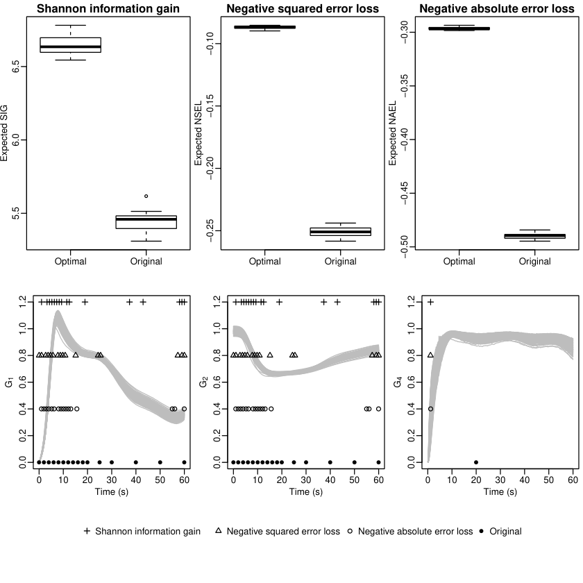
We use the methodology from Section 3.2 and the ACE algorithm to find designs that maximize each of the NSEL, NAEL and SIG utilities. We compare these designs to the original design used by Swameye et al. (2003). As in the previous examples, we introduce the constraint that the observation times need to be at least 1 second apart, a requirement also satisfied by the original experiment. Figure 4 presents boxplots of twenty evaluations of the Monte Carlo approximation to the expected utility for the original design and the optimal designs found under each utility function. Once again, in each case, the optimal designs are considerably more efficient. Also shown in Figure 4 are the four designs under comparison. The optimal designs favor having a dense set of points early in the observation window, and then a smaller set of times near the end of the experiment. This is especially true for the designs under NSEL and NAEL where 75% of the observation times occur before seconds, compared to about 60% for SIG design and 50% for the original design. Early observation times provide information about the peak in and the sharp decrease in at about 10 seconds. For the single observation time, , on , the optimal designs clearly favor making a very early observation. Note that for each of the optimal designs is between 1 and 2 seconds.
Application: transport of serine across human placenta
We now use the methodology in Section 3 to redesign the experiment for the human placenta study introduced in Section 1. The experimental protocol specifies fixed initial amounts of radioactive serine interior () and exterior () to the placenta ( and l, respectively). The original design proposed by the experimenters used placentas (runs) with differing amounts of non-radioactive serine interior () and exterior () to the placenta, see Table 1. Noisy observations on the amount of interior radioactive serine () were made at eight times, common to each of the seven placentas. The experimenters expected greater variability in the concentration of interior radioactive serine near the start of the experiment, before convergence to an equilibrium. Therefore, they choose a design containing a large number of early time points. We broadly follow this protocol, but find optimal designs using placentas with each having observations taken at common times, , chosen from across the interval .
A hierarchical statistical model is assumed for the observed responses:
where , are independent and identically normally distributed with constant variance , and holds the subject-specific parameters for the th placenta with elements assumed to follow independent uniform distributions
The goal of the experiment is estimation of the population physical parameters .
A priori, we assume and , where denotes the symmetric triangle distribution on the interval . Reflecting prior knowledge from previous experiments, we set , , , and we assume for the response variance.
We expect the solution to system of equations (2) to be smooth, and so use squared exponential covariance (8) for the probabilistic solution. The evaluation grid, , has size and we set auxiliary correlation parameter .
Specifying a design corresponds to specifying the experimental conditions , initial values , and the common observation times . Hence for , the design space has between 12 and 22 dimensions. As for the examples in Section 4, we impose a constraint on the observation times and specify that they must be at least 5 seconds apart.
We find designs for the NSEL, NAEL, 0-1 estimation and 0-1 model selection utility functions defined in Section 3.1. For the 0-1 estimation utility, we set ; for utility to equal 1, the posterior mean for must lie in the box set , which contains 0.5% of the volume of the prior support. For the model selection utility, we suppose interest is in determining if the reaction rates are equal, i.e. does ? To answer this question, we define two models: (where ) and (where ).
Figure 5 presents boxplots of twenty evaluations of the Monte Carlo approximation to the expected utility for the optimal design found under each utility function for . We also present boxplots of the performance of the original design with . Unsurprisingly, the expected utility increases with , and the optimal designs are clearly superior to the original design. For each utility function, the optimal design with outperforms the original design with placentas, with substantial differences in expected utility.
| NSEL | NAEL | Est01† | MS01⋆ | Original | ||||||
|---|---|---|---|---|---|---|---|---|---|---|
| Placenta | ||||||||||
| 1 | 0 | 0 | 0 | 0 | 0 | 0 | 0 | 0 | 0 | 0 |
| 2 | 0 | 38 | 0 | 0 | 0 | 0 | 0 | 0 | 250 | 0 |
| 3 | 0 | 50 | 0 | 50 | 0 | 56 | 0 | 0 | 250 | 250 |
| 4 | 0 | 68 | 0 | 67 | 0 | 58 | 0 | 0 | 250 | 1000 |
| 5 | 182 | 1000 | 160 | 1000 | 177 | 1000 | 0 | 38 | 1000 | 0 |
| 6 | 185 | 1000 | 175 | 1000 | 196 | 1000 | 0 | 41 | 1000 | 250 |
| 7 | 206 | 1000 | 211 | 1000 | 210 | 1000 | 115 | 62 | 1000 | 1000 |
† 0-1 estimation utility; ⋆ 0-1 model selection utility
Table 1 gives the treatments for each design found for . Figure 6 shows the observation times for the optimal designs under NSEL, NAEL and 0-1 estimation utilities, along with realizations from the solution to , for each run of each design. The designs under NSEL and NAEL utilities have similar treatments and observation times. The initial concentrations in Table 1 lead to three distinct profiles of (labeled placentas 1 and 2; 3 and 4; 5, 6 and 7; note though that the placentas are exchangeble). The profile for placentas 1 and 2 has a slow steady increase in with respect to . Placentas 3 and 4 have a steep initial increase and subsequent decrease in with respect to . Finally, placentas 5 to 7 have a steep initial increase in with respect to followed by a slow decrease. The optimal observation times are predominantly at the beginning of the observation window, where is changing most quickly. The designs under the 0-1 estimation utility are also similar, except a non-zero amount (35 l) of the initial interior non-radioactive serine is applied to placenta 2.

Figure 7 shows the designs from the 0-1 model selection utility, along with realizations of the solutions under models and . The treatments for the optimal design under the 0-1 utility result in two distinct profiles of . For placentas 1–5, has a slow steady increase in with respect to . Placentas 6 and 7 have a steep initial increase and subsequent decrease in with respect to . Unlike the other optimal designs, the observation times are predominantly towards the end of the observation window. The profiles are similar under both models, with the most substantial differences occurring in the inter-profile variability towards the middle of the time interval. This region is where the majority of observation times are located.
The original design proposed by the experimenters had an unequal spacing of observation times across the entire interval . There are more observations taken near the start of the interval, and the time points are not dissimilar to those in the optimal designs under NSEL, NAEL and 0-1 estimation. However, the original design has treatments that are very different from any of the optimal designs, with an almost factorial structure and some treatments with high values of (exterior initial concentration of non-radioactive serine). None of the optimal designs include treatments with high , demonstrating how it is often difficult to predict by intuition the treatments in a Bayesian optimal design for a complicated nonlinear model. In addition, the designs for point estimation (under NSEL, NAEL and 0-1 estimation utilities) are quite different to the design for model selection.
Concluding Remarks
This paper introduces and demonstrates the first practical methodology for Bayesian optimal design of experiments for statistically nonlinear models formed from the solution to intractable ordinary differential equations. The work is motivated by a challenging design problem from the biological sciences, which we address through a combination of probabilistic solutions to the equations, simulation-based approximation to expected utilities and optimization via smoothing and cyclic descent. Our novel adjustments to the Chkrebtii et al. (2016) probabilistic algorithm are key to providing a computationally efficient solution to the optimal design problem. Through demonstration on a number of examples, including the motivating experiment on serine transport across placental membranes, we show the efficiency gains that can be made by use of optimal designs over obvious, and proposed, alternatives. We also show how it is often not possible to “second guess” via intuition the solutions to optimal problems for nonlinear models.
We have adopted the nested integration and optimization methods from Overstall and Woods (2017) to find optimal designs for the differential equation models in this paper (namely the ACE algorithm). The Markov chain simulation schemes of Müller (1999) and Müller et al. (2004), among other authors, would be an interesting alternative approach. Extension and application of such methods to the problems in the current paper is an area for future research.
One key issue not addressed is model discrepancy (see, e.g., Kennedy and O ’Hagan, 2001 and Plumlee, 2017); the systematic mis-match between the true physical process and the solution to the ordinary differential equations. Not taking account of this error can lead to significant bias in posterior estimates of the physical parameters (Brynjarsdottir and O ’Hagan, 2014). Future work will focus on Bayesian optimal design for physical models subject to model discrepancy.
Some limited insight into the impact of model mis-match can be gained from a simple extension to the compartmental model in Section 4.2. For the purpose of finding designs, we assume the model
| (11) |
That is, we simplify (10) by setting and equal to their prior means in the fraction that multiplies the exponential term. We still assume the exponential depends on unknown , and assume the same prior distributions for all parameters as in Section 4.2.
To assess the impact of model mis-match, we find optimal designs under the SIG, NSEL and NAEL utilities assuming the misspecified model (11). We then assess these designs under the correct, more complex, model (10) and compare them to designs found under the correct model by evaluating the approximate expected utility under the correct model, see Figure 8. Differences in approximate expected utility between the designs found under the correct and misspecified models are comfortably within Monte Carlo error for SIG. However, assuming a misspecified model under the NSEL utility results in a loss of expected utility of around 6%; the differences are somewhat less for NAEL but still larger than Monte Carlo error. Clearly, the reduction in expected utility from assuming a misspecified model will depend on the models under consideration, the difference between the models and the choice of prior distributions, in addition to the choice of utility function. This is an important area for future research.
Acknowledgements
We thank Rohan Lewis, Bram Sengers and Nont Panitchob from Medicine, Life Sciences and Bioengineering at the University of Southampton for providing details of the placenta experiment. We are grateful to two anonymous reviewers whose comments improved the paper.
Funding
The second author was supported by Fellowship EP/J018317/1 from the United Kingdom Engineering and Physical Sciences Research Council.
Appendix A The ACE algorithm
In Algorithm 4, we outline the basic approximate coordinate exchange algorithm. For full details, see Overstall and Woods (2017).
Let be the total number of coordinates (values taken by each variable in each run) of the design. That is, is the dimension of the design. In step 4, the probability of the suggested design having higher expected utility is calculated, a posteriori to two independent Monte Carlo samples from the joint distributions of the data and parameters conditional on the current and suggested designs. Calculation of this probability assumes the utility evaluations are well described by a normal distribution. In the case of 0-1 utilities, a similar test based on a Bernoulli likelihood and Beta prior is applied (see Overstall et al., 2018a for details). Convergence in step 4 is assessed informally using trace plots of the evaluations of either , if the proposed design was accepted, or , otherwise, from step 4.
The ACE algorithm should be started from multiple different starting designs . From the resulting designs, the one with the lowest value of should be returned.
References
- Atkinson and Bogacka (2002) Atkinson, A. C. and Bogacka, B. (2002), “Compound and other opimum designs for systems of nonlinear differential equations arising in chemical kinetics,” Chemometrics and Intelligent Laboratory Systems, 61, 17–33.
- Atkinson et al. (1993) Atkinson, A. C., Chaloner, K., Herzberg, A. M., and Juritz, J. (1993), “Experimental designs for properties of a compartmental model,” Biometrics, 49, 325–337.
- Brynjarsdottir and O ’Hagan (2014) Brynjarsdottir, J. and O ’Hagan, A. (2014), “Learning about physical parameters: the importance of model discrepancy,” Inverse Problems, 30, 114007.
- Chaloner and Verdinelli (1995) Chaloner, K. and Verdinelli, I. (1995), “Bayesian experimental design: a review,” Statistical Science, 10, 273–304.
- Chkrebtii et al. (2016) Chkrebtii, O. A., Campbell, D. A., Calderhead, B., and Girolami, M. A. (2016), “Bayesian uncertainty quantification for differential equations,” Bayesian Analysis, 11, 1239–1267.
- FitzHugh (1961) FitzHugh, R. (1961), “Impulses and physiological states in models of nerve membrane,” Biophysical Journal, 1, 445–466.
- Franceschini and Macchietto (2008) Franceschini, G. and Macchietto, S. (2008), “Model-based design of experiments for parameter precision: state of the art,” Chemical Engineering Science, 63, 4846–4872.
- Holsclaw et al. (2013) Holsclaw, T., Sansó, B., Lee, H. K. H., Heitmann, K., Habib, S., Higdon, D., and Alam, U. (2013), “Gaussian process modeling of derivative curves,” Technometrics, 55, 57–67.
- Iserles (2009) Iserles, A. (2009), A First Course in the Numerical Analysis of Differential Equations, Cambridge University Press.
- Kennedy and O ’Hagan (2001) Kennedy, M. C. and O ’Hagan, A. (2001), “Bayesian calibration of computer models (with discussion),” Journal of the Royal Statistical Society B, 63, 425–464.
- Lange (2013) Lange, K. (2013), Optimization, New York: Springer, 2nd ed.
- Meyer and Nachtsheim (1995) Meyer, R. K. and Nachtsheim, C. J. (1995), “The coordinate-exchange algorithm for constructing exact optimal experimental designs,” Technometerics, 37(1), 60–69.
- Müller (1999) Müller, P. (1999), “Simulation-based optimal design,” in Bayesian Statistics 6, eds. Bernardo, J. M., Berger, J. O., Dawid, A. P., and Smith, A. F. M., Oxford: Oxford University Press, pp. 459–474.
- Müller and Parmigiani (1996) Müller, P. and Parmigiani, G. (1996), “Optimal design via curve fitting of Monte Carlo experiments,” Journal of the American Statistical Association, 90, 1322–1330.
- Müller et al. (2004) Müller, P., Sanso, B., and De Iorio, M. (2004), “Optimal Bayesian design by inhomogeneous Markov chain simulation,” Journal of the American Statistical Association, 99, 788–798.
- Nagumo et al. (1962) Nagumo, J., Arimoto, S., and Joshizawa, S. (1962), “An active pulse transmission line simulating a nerve axon,” Proceedings of the Institute of Radio Engineers, 50, 2061–2070.
- Overstall et al. (2018a) Overstall, A. M., McGree, J. M., and Drovandi, C. C. (2018a), “Fully Bayesian design using the approximate coordinate exchange algorithm and normal-based approximations to posterior quantities,” Statistics and Computing, 28, 343–358.
- Overstall and Woods (2017) Overstall, A. M. and Woods, D. C. (2017), “Bayesian design of experiments using approximate coordinate exchange,” Technometerics, 59, 458–470.
- Overstall et al. (2018b) Overstall, A. M., Woods, D. C., and Adamou, M. (2018b), “acebayes: An R package for Bayesian optimal design of experiments via approximate coordinate exchange,” arXiv:1705.08096.
- Overstall et al. (2018c) — (2018c), acebayes: Optimal Bayesian experimental design using the ACE algorithm, R package version 1.6.0.
- Panitchob et al. (2015) Panitchob, N., Widdows, K. L., Crocker, I. P., Hanson, M. A., Johnstone, E. D., Please, C. P., Sibley, C. P., Glazier, J. D., Lewis, R. M., and Sengers, B. G. (2015), “Computational modelling of amino acid exchange and facilitated transport in placental membrane vesicles,” Journal of Theoretical Biology, 365, 352–364.
- Pellegrini and Dusanter-Fourt (1997) Pellegrini, S. and Dusanter-Fourt, I. (1997), “The structure, regulation and function of the Janus kinases (JAKs) and the signal transducers and activators of transcription (STATs),” European Journal of Biochemistry, 248, 615–633.
- Plumlee (2017) Plumlee, M. (2017), “Bayesian calibration of inexact computer models,” Journal of the American Statistical Association, 112, 1274–1285.
- Ramsay et al. (2007) Ramsay, J., Hooker, G., Campbell, D., and Cao, J. (2007), “Parameter estimation for differential equations: a generalised smoothing approach (with discussion),” Journal of the Royal Statistical Society B, 69, 741–796.
- Rasmussen and Williams (2006) Rasmussen, C. E. and Williams, C. K. I. (2006), Gaussian Processes for Machine Learning, Cambridge, MA.: MIT Press.
- Raue et al. (2009) Raue, A., Kreutz, C., Maiwald, T., Bachmann, J., Schilling, M., Klingmuller, U., and Timmer, J. (2009), “Structural and practical identifiability analysis of partially observed dynamical models by exploiting the profile likelihood,” Bioinformatics, 25, 1923–1929.
- Rodríguez-Díaz and Sánchez-León (2014) Rodríguez-Díaz, J. M. and Sánchez-León, G. (2014), “Design optimality for models defined by a system of ordinary differential equations,” Biometrical Journal, 56, 886–900.
- Ryan et al. (2014) Ryan, E., Drovandi, C., Thompson, M., and Pettitt, A. (2014), “Towards Bayesian experimental design for nonlinear models that require a large number of sampling times,” Computational Statistics and Data Analysis, 70, 45–60.
- Ryan et al. (2016) Ryan, E. G., Drovandi, C. C., McGree, J. M., and Pettitt, A. N. (2016), “A review of modern computational algorithms for Bayesian optimal design,” International Statistical Review, 84, 128–154.
- Ryan (2003) Ryan, K. J. (2003), “Estimating expected information gains for experimental designs with application to the random fatigue-limit model,” Journal of Computational and Graphical Statistics, 12, 585–603.
- Sacks et al. (1989) Sacks, J., Welch, W. J., Mitchell, T. J., and Wynn, H. P. (1989), “Design and analysis of computer experiments (with discussion),” Statistical Science, 4, 409–435.
- Santner et al. (2003) Santner, T. J., Williams, B. J., and Notz, W. I. (2003), The Design and Analysis of Computer Experiments, New York: Springer.
- Solak et al. (2003) Solak, E., Murray-Smith, R., Leithead, W. E., Leith, D. J., and Rasmussen, C. E. (2003), “Derivative observations in Gaussian process models of dynamic systems,” in Advances in Neural Information Processing Systems, eds. Becker, S., Thrun, S., and Obermayer, K., MIT Press, vol. 15, pp. 1057–1064.
- Swameye et al. (2003) Swameye, I., Muller, T., Timmer, J., Sandra, O., and Klingmuller, U. (2003), “Identification of nucleocytoplasmic cycling as a remote sensor in cellular signaling by databased modeling,” Proceedings of the National Academy of Sciences, 100, 1028–1033.
- Valko and Vajda (1984) Valko, P. and Vajda, S. (1984), “An extended ODE solver for sensitivity calculations,” Computers and Chemistry, 8, 255–271.
- Widdows et al. (2017) Widdows, K. L., Panitchob, N., Crocker, I. P., Please, C. P., Hanson, M. A., Sibley, C. P., Johnstone, E. D., Sengers, B. G., Lewis, R. M., and Glazier, J. D. (2017), “Integration of computational modeling with membrane transport studies reveals new insights into amino acid exchange transport mechanisms,” The FASEB Journal, in press.
- Woods et al. (2017) Woods, D. C., Overstall, A. M., Adamou, M., and Waite, T. W. (2017), “Bayesian design of experiments for generalised linear models and dimensional analysis with industrial and scientific application (with discussion),” Quality Engineering, 29, 91–118.