Checking T and CPT violation with sterile neutrino
, , ,
1234Department of Physics, University of Lucknow, Lucknow 226007 India
Abstract
Post LSND results, sterile neutrinos have drawn attention and motivated the high energy physics, astronomy and cosmology to probe physics beyond the standard model considering minimal 3+1 (3 active and 1 sterile) to 3+N neutrino schemes. The analytical equations for neutrino conversion probabilities are developed in this work for 3+1 neutrino scheme. Here, we have tried to explore the possible signals of T and CPT violations with four flavor neutrino scheme at neutrino factory. Values of sterile parameters considered in this analysis are taken from two different types of neutrino experiments viz. long baseline experiments and reactor+atmospheric experiments. In this work golden and discovery channels are selected for the investigation of T violation. While observing T violation we stipulate that neutrino factory working at 50 GeV energy have the potential to observe the T violation signatures for the considered range of baselines(3000 km-7500 km). The ability of neutrino factory for constraining CPT violation is enhanced with increase in energy for normal neutrino mass hierarchy(NH). Neutrino factory with the exposure time of 500 kt-yr will be able to capture CPT violation with GeV at 3 level for NH and for IH with GeV at 3 level.
Keywords : sterile neutrinos, T violation, CPT violation, neutrino factory
Acknowledgements
One of the authors Sujata Diwakar is thankful to University Grant Commission,India for giving financial support under the Rajiv Gandhi National Fellowship scheme.
1 Introduction
The standard model of particle physics considers neutrinos to be massless. Sudbury Neutrino Observatory[1][2] gave evidence of neutrino oscillations which was further confirmed by KamLAND experiment [3]. This landmark research assigned mass to the neutrinos and gave a clear indication of new physics beyond the standard model. A simple stretch in the standard model was able to stand up with the mass of neutrino.
In neutrino physics the standard three flavour neutrino oscillations can be explained with the help of six parameters namely , , , , and . Amongst these six parameters, solar parameters(, ) and atmospheric parameters () have been measured with high precision. Furthermore, Daya Bay and RENO reactor experiments have strongly constrained the value of mixing angle . Now we are in need of such neutrino experiments which can impose tight constraints on the value of and mass hierarchy. Some anomalies popped up while observing appearance channel and disappearance channel of at LSND experiment. While observing appearance channel, LSND [4] [5] [6] [7] [8] [9] was the first experiment to publish evidence of a signal at . Later in 2002, MiniBooNE [10] [11] checked the LSND result for () appearance channel. In MiniBooNE experiment, while observing the CCQE events rate through above 475 MeV energy, no excess events were found but for energies 475 MeV excess events were observed. In this way, MiniBooNE supported the LSND result. The LEP data[12][13] advocates the number of weakly interacting light neutrinos, that couple with the Z bosons through electroweak interactions, to be 2.984 0.008; thus closing the door for more than three active neutrinos. Hence, the heavy neutrino announced by LSND group should be different from these three active neutrinos. This higher mass splitting in the standard three active neutrino model was accommodated by introducing sterile neutrinos. Sterile neutrinos carry a new flavor which can mix up with the other three flavors of standard model but they do not couple with W and Z bosons. The number of sterile neutrinos can vary from minimum one to any integer N.
Some cosmological evidences like CMB anisotropies [14] [15] [16] [17] [18] and Big Bang nucleosynthesis [19] [20] also stood up with the LSND data. The results reported by the combined analysis [21] of Baryonic Acoustic Oscillations(BAO) ‘+PlaSZ+Shear+RSD’ indicated the presence of sterile neutrinos by stipulating the number of effective neutrinos , and giving preference for at 1.4 level and non zero mass of sterile neutrino at 3.4 level.
The gallium solar neutrino experiments(gallium anomaly) GALLEX [27], SAGE [28] and the antineutrino reactor experiments () like Bugey-3, Bugey-4, Gosgen, Kransnogark, IIL [29] (reactor anomaly) indicated that electron neutrinos and antineutrinos may disappear at short baselines. Such disappearance can be explained by the presence of at least one massive neutrino (of the order of 1 eV). Thus, these experiments also indicated the presence of sterile neutrino and supported the LSND results. Some constraints imposed by the combined fit of reactor, gallium, solar and scattering data are and at 95% CL [30]. Few atmospheric neutrino experiments such as IceCube [31], MINOS [32] [33] [34], CCFR [35] have also imposed strong constraints on sterile parameters.
The four flavors of neutrino can be studied in either of the two different neutrino mass schemes, 3+1 or 2+2 schemes[36]. For our work we have selected (3+1) four flavor neutrino mass scheme. In this framework, Maki-Nakagawa-Sakata (MNS) mixing matrix (), includes six mixing angles , three dirac phases and three majorana phases. In our analysis majorana phases are not taken into consideration.
Neutrino factory [37][38] provides excellent sensitivity to the standard neutrino oscillation parameters and therefore seems to be one of the promising option to explore and reanalyze the global fits for sterile neutrino parameters too. To mention, it provides a platform to constrain one of the most searched CP violation in leptonic sector [39][40]. Hence neutrino factory seems to provide a promising environment for the study of T and CPT violation. The neutrino factory set up considered here is based on the International Design Study of Neutrino Factory [IDS-NF] [41][42]. From the measure of we can not directly constrain CP phase because the value of in the presence of matter will contain in itself some CP odd effects even in the absence of CP phase. Therefore, instead of checking , variation in can be studied to probe extent of true CP violation. We have observed T violation through golden channel and discovery channel and CPT violation along disappearance channel.
Our work is organized as follows.
In section 2, we illustrate 3+1 neutrino matrix parametrization. In next section, T violating effects are checked for different channels. In section 4, bounds on CPT violating terms are checked in presence of sterile neutrino. In the last section, we have summarized our study and discussed the results observed.
2 Standard Parametrization in 3 + 1 neutrino scheme
The 3 (active) + 1 (sterile) neutrino scheme can be looked upon as 3+1 or 2+2 scheme depending on the selection of mass ordering of the neutrinos. To check T and CPT violation we have selected
3+1 scheme for our analysis. In this scheme the flavor eigenstates and mass eigenstates are related by the given unitary transformation equation
| (1) |
Here unitary matrix (U) can be parametrized in terms of six mixing angles(), three Dirac phases () and three majorana phases. Majorana phases are neglected in our study as they do not affect the neutrino oscillations in any realistically observable way. In principle, there are different parametrization schemes for the neutrino mixing matrix as their order of sub-rotation is arbitrary. Our selection for parametrization of neutrino mixing matrix is
| (2) |
where are the complex rotation matrices in the ij plane, defined as
| (3) |
The order of rotation between 14 and 23 is arbitrary since these matrices commute. When neutrinos pass through the earth matter, the charge current interactions (CC) of and neutral current interactions (NC) of with the matter give rise to a CC and NC potentials and respectively. While studying the sterile neutrinos, potential can not be neglected. The effective CPT violating hamiltonian () of neutrinos can be expressed as
| (4) |
Here , and . is the Fermi constant, and are the number density of electrons and neutrons respectively with in earth matter. The ’s are CPT violating terms. Different angular values for unitary matrix are checked in [43]. In our work we have considered . Hamiltonian can be diagonalized to by an unitary matrix . This can be expressed as
| (5) |
The matrix elements will represent the eigenvalues of . Full analytical expressions for neutrino oscillation probabilities are developed in this work by using time independent perturbation theory. In an attempt to apply perturbation we have defined few oscillation parameters in terms of perturbative parameter , where . The neutrino oscillation parameters can be rewritten as
We treat . Now the Hamiltonian can be written as
| (6) |
where , and are the hamiltonians corresponding to zeroth, first and second order in respectively. The evolution equation for neutrino oscillation probability is defined as
| (7) |
where is the evolution matrix of neutrino which is also called oscillation probability amplitude
| (8) |
The evolution matrix of neutrinos in terms of eigenvalues of can be written as
| (9) |
where
From equation (7) the neutrino oscillation probability from flavor to flavor can be written as
| (10) |
This is the general form of equation for neutrino oscillation probability.
3 T violation in (3+1) framework
In neutrino oscillations the flavor conversion probabilities from flavor to flavor can be written as
| (11) |
Redefining the above probability equation as sum of and terms
| (12) |
CP even terms are CP conserving and can be written as
| (13) |
CP odd term are CP violating and can be written as
| (14) |
Assuming CPT to be conserved, the magnitude of CP violation will be equal to the magnitude of T violation , i.e.
| (15) |
therefore we can write
| (16) |
When neutrinos passes through the earth matter, the interaction of neutrinos with matter gives rise to an extra potential. This potential is positive for neutrinos and negative for antineutrinos leading to different eigenvalues of hamiltonian for them. Further, this difference in hamiltonian for ’s and ’s give rise to fake(extrinsic) CP violation. Hence, check on T violation appears to be a better choice in the presence of matter. From equation (16) the T violation can be looked upon as
| (17) |
If we consider and the above equation becomes
| (18) |
The term is known as Jarlskog factor and are energy eigenvalues of hamiltonian in matter.
| (19) |
The energy eigenvalues in matter can be connected to the energy eigenvalues in vacuum by the relations , , and . The terms ,, , in matter can be calculated with the help of the terms , ,, in vacuum (where ) using the following expressions [44].
| (20) |
| (21) |
| (22) |
| (23) |
where
| (24) |
| (25) |
is the diagonal element of the matter potential matrix in four neutrino scheme and A is the diagonal element of matter potential matrix in three neutrino scheme. Since T violating effects can only be studied in appearance channels so . In an effort to put constraints on we have studied two appearance channels. These are (golden channel) and (discovery channel).
The T violation probability difference expression for the golden channel can be expressed as
| (26) |
Since large value of gives rise to rapid oscillations, hence terms can be averaged out. Solving the above expression up to the power we get
| (27) |
| (28) |
is matter dependent term. The change in will change the value of .
Further we have developed equation of for discovery channel. The discovery channel is not very useful in the standard three neutrino flavor framework, nevertheless while studying physics beyond three active neutrino flavor framework, it becomes very important. For discovery channel() the probability difference is given as
| (29) |
Solving the above expression up to the power we get,
| (30) |
| (31) |
The for three neutrino framework [45] is given by
| (32) |
Keeping the best fit values of neutrino oscillation parameters and assigning maximum value to dirac phases i.e keeping mod of sin of dirac phases to be unity will lead us to maximum value of . This assumption will render the maximum limit on the bounds which can be imposed on T violation arising due to the presence of dirac phases if all other oscillation parameters are known with utmost accuracy. From equation (32) gives the value of for three neutrino flavor framework [46]. This value is independent of the selection of probing channel and presence of matter effects. Whereas in 4 flavor framework it will depend on the selection of channel through which we want to probe CP or T violation and it will vary with matter effects too. Within 4 flavor neutrino framework the magnitude of will depend on active flavor neutrino mixing angles (known with accuracy), sterile neutrino mixing angles (still needs better bounds), matter effects, baseline, energy and dirac phases (not known) . Imposition of constraints on dirac phase (three neutrino flavor) or phases (four neutrino flavor) is still in research phase.

(a)Variation in along the baseline

(b)Variation in along the baseline
The probability differences in neutrino sector are represented by equations (28) and (31) for and channels respectively. The values of sterile parameters used in the above mentioned equations are taken from
(i) long baseline neutrino oscillation experiments [47]
, and
(ii) short baseline reactor and atmospheric experiments [48] [49]
, and
The variations in and are checked along the baseline for two different energies i.e 4 GeV and 50 GeV. Plot (a) of Figure 1 reflects a very small variation in in comparison to for golden channel when it is checked with two different energies and two sets of sterile parameter values. Plot (b) of Figure 1 reflects a reasonable variation in in comparison to for discovery channel when it is checked for 50 GeV energy and sterile parameters are taken from reactor+atmospheric experiments. The comes up as the promising channel to observe the signatures of T violation. From the analysis we conclude that neutrino factory operating at 50 GeV has the potential to capture the signatures of T violation through channel if true sterile parameter values are equal to that taken from reactor+atmospheric experiments. At the same time if the upcoming neutrino experimental setups captures value above 0.137 then we can stipulate presence of some new physics beyond three active flavor neutrino physics which is responsible for the enlargement observed in value.
4 CPT violation in 3 + 1 scheme
CPT invariance is one of the most fundamental symmetries of nature. CPT conservation indicates the invariance in the properties of physical quantities under the discrete transformations such as charge conjugation (C), parity inversion (P) and time reversal (T) along with the invariance under lorentz transformation. CPT invariance is one of the symmetries of local quantum field theory which implies that there is an important relation between CPT invariance and Lorentz invariance. If CPT invariance is violated, Lorentz invariance must violate but if Lorentz invariance is violated it is not necessary that CPT invariance must violate. In our work disappearance channel is probed to check CPT violation. The CPT violating probability difference can be written as
| (33) |
The intrinsic CPT violation arises due to the violation of CPT invariance theorem. A hamiltonian containing CPT violating terms is defined by equation (4) and the general form of neutrino oscillation probability is mentioned in equation (10). The terms and of the expression (10) are the elements of the unitary matrix . The construction of unitary matrix with the help of eigenvalues and eigenvectors of hamiltonian , and is mentioned in the Appendix. After the formation of unitary matrix , we have developed the neutrino oscillation probability equations up to second order in . Since is large, so we average out the effects produced due to in the probability equations. Neutrino oscillation probabilities for different oscillation channels containing CPT violating parameters can be developed as
| (34) |
| (35) |
| (36) |
| (37) |
| (38) |
For small angles () these oscillation probabilities can be written as
| (39) |
| (40) |
| (41) |
| (42) |
| (43) |
In order to analyse CPT violation at probability level in 4 flavor neutrino framework the value of considered in our analysis is given by
| (44) |
![[Uncaptioned image]](1509.04096v3/longnormal.png)
(a)
![[Uncaptioned image]](1509.04096v3/reactornormal.png)
(b)

(c)
(d)

(a) Normal hierarchy

(b) Inverted hierarchy
Neutrino factory setup considered for analysing CPT violation is taken from the references [50][51][52][53] and [54]. The experimental setup and detector specifications considered in our analysis are mentioned below. Neutrino factory setup consist of useful muon decays per polarity, with parent muon energy . We have done our analysis for 10 years running of neutrino factory. In particle physics meaningful observations always demands a detector with very good energy and angular resolutions. This view point lead us to select Liquid Argon detector for particle detection. The energy resolution of the detector for muon is .
A near detector is placed at a distance 20 m from the end of the decay straight of the muon storage ring. Effective baseline () is used in place of baseline (L), which is calculated using [55]. Fiducial mass of near detector is 200 tons. Presence of near detector will minimize the systematic uncertainties in our observations.
A 50 Kt far detector is placed at a distance of 7500 Km. The systematic uncertainties considered for this analysis are given in Table 1. An uncertainty of 5% on matter density [56][57] is also considered in our work . The simulated environment of the neutrino factory is created with the help of GLoBES [58] [59]. The analytical equations for four flavor neutrino conversion probabilities derived in this work are defined in the probability engine of the software. The best fit values of oscillation parameters [47] [60] are mentioned in Table 2. Sterile parameter values mentioned in the Table 2 represents best fit values for =0.1 .
| Systematic uncertainties | values |
| Flux normalization | 2% |
| Fiducial mass errors for near detector | 0.6 % |
| Fiducial mass errors for far detector | 0.6 % |
| energy calibration error for near detector | 0.5 % |
| energy calibration error for far detector | 0.5 |
| shape error | 10 % |
| Backgrounds |
| Parameter | Best fit values |
|---|---|
| ; | |
| ; | |
| ; | |
The constraints on CPT violating parameters and within two and three neutrino frameworks are mentioned in references
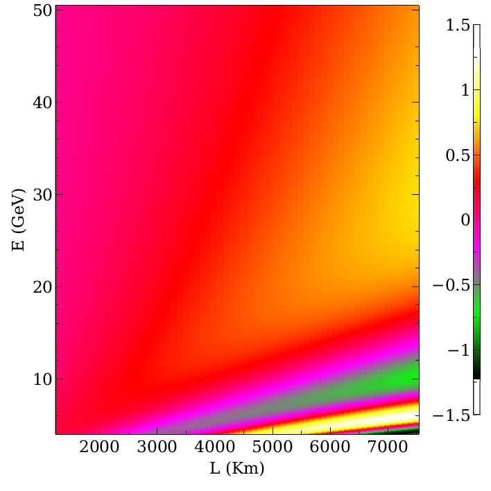
[43] [61] [62] [63] [64] [65] and [66]. In present work we are trying to check the neutrino factory potential to capture CPT violating signatures in presence of sterile neutrino. As the mass hierarchy determination is yet in research phase therefore in an attempt to make this work relevant we have analysed CPT invariance for both the mass hierarchies. Initially CPT violating signatures are checked at probability level. The value of is estimated by substituting equation (41) in equation (44) for the channel . The variation in and with baseline and energy is shown in Figure 2 and Figure 3 oscillographs respectively. The total CPT violation captured by any experiment will be the sum of extrinsic CPT violation (CPT violation arising due to matter effects) and intrinsic or genuine CPT violation(which we are probing in present work). In an endeavour to constraint intrinsic CPT violating parameters we must look for places where extrinsic CPT violation is negligible or very less. With three active neutrinos the extrinsic CPT violation is checked in reference [67] whereas with 3 (active) + 1 (sterile) neutrinos it is checked in reference [68]. These references conclude that extrinsic CPT violation for energies 4 GeV- 6 GeV is negligible at shorter baselines, roughly less than 2000 km. Whereas for longer baselines this effect decreases with energy. Equation (44) of our work will check the presence of pure CPT violation arising in the presence of sterile neutrino at probability level. The values of CPT violating parameters considered while plotting oscillographs are GeV and GeV. Looking at normal and inverted hierarchy oscillographs(Figure 2) we can observe the presence of pure CPT violating signatures at shorter baselines i.e. from 1300 km-2000 km for 4 GeV-6 GeV energies. The references [67] [68], which speak about extrinsic CPT violation have recorded very weak or almost negligible signatures of extrinsic CPT violation at the above mentioned energies and baselines. Hence baselines from 1300 km-2000 km with neutrino energies in the range 4 GeV-6 GeV are favourable for probing CPT violation with neutrino factory. In Figure 2 while looking at normal hierarchy oscillographs we observe =-0.05 along baselines 4000 km-7500 km for energies 12 GeV-30 GeV. The inverted hierarchy oscillographs of the same Figure captures =0.25 and 1 for sterile parameters taken from long baseline experiments and reactor+atmospheric experiments respectively. This probability difference can be observed for baselines 4000 km-7500 km and energies 20 GeV-50 GeV.
After examining the presence of pure CPT violation at probability level we go ahead to observe the signatures of the same with realistic proposed neutrino experiments i.e. neutrino factory. The specifications of neutrino factory considered in our work are mentioned earlier. Liquid argon detector seems a reasonable choice to grab the signatures of leptons in the considered energy range. The rate(event) level analysis depends on mathematical formulation( oscillation probability), physics(types of interactions) and R & D (source properties and detector properties) of the experiment. Looking at equations (34) to (44) we found that appears with term and term appears with term. The solar and atmospheric mass square difference ( and ) are of the order of and respectively. Hence, any change in mass terms due to the presence of CPT violating parameter will be better observed in term.
To hook CPT violating impression with neutrino factory we have investigated some observable parameters like R, and asymmetry factor. These terms are defined by equations (45) and (46). The ratio R and ratio difference are examined as
| (45) |
where denotes number of muon neutrinos reaching at detector as muon neutrinos and producing a lepton and denotes number of anti muon neutrinos reaching at detector as anti muon neutrinos and producing a lepton. In , denotes the ratio R in presence of CPT violating terms and denotes the ratio R in absence of CPT violating terms.

(a)

(b)

(a)

(b)

(a)

(b)

(a)

(b)
In presence of matter the observable R will not be equal to one, even if pure CPT violation is absent. It will be equal to a numerical value representing the ratio of neutrino and antineutrino interaction cross-sections. If we want to analyse the extent of deviation produced by pure CPT violation, we have to hide or filter out the deviation produced by any other phenomenon. In an attempt to filter out pure CPT violating contribution from the total observed deviation we take into record a new observable . This parameter is defined in the equation (45). Figures 4 and 6 demonstrate the variation in R with energy whereas Figures 5 and 7 exhibit variation in with energy for baseline 7500 km. We observe that at long baselines pure CPT violating effects get smaller with increase in energy. The presence of CPT violation signatures can be observed with neutrino factory and it can be checked by looking R and plots (Figure 4- Figure 7) for different values of CPT violating parameter . As we know that in presence of sterile neutrino the manifestation of pure CPT signatures depends on the values of sterile parameters, hence the entire analysis is performed with two sets of best fit values of sterile parameters which were examined by different neutrino experiments. The results from neutrino factory with sterile parameter values obtained from reactor+atmospheric experiments exhibit larger deviation in observables R and in comparison to the results obtained with sterile parameter values taken from long baseline experiments. These observables are checked for both mass hierarchies. From the Figures 4,5,6 and 7 we comprehend that after 15 Gev there is a flip in sign of the observables for both the hierarchies. At the same time the amount of deviation measured for pure CPT violating effects are different for NH and IH for the same energy and baseline.
The next observable asymmetry factor is defined as
| (46) |
This ratio is determined by using far and near detectors. The variations in asymmetry factor with energy for baseline 7500 km are shown by Figures 8 and 9. These figures reflect the variations in observable for different values of (CPT violating parameter) and for both mass hierarchies. The =0 will reflect values without any contribution from CPT violating terms. The asymmetry factor increases with the increase in the value of . An enhancement in magnitude of asymmetry factor is also observed with the increase in values of sterile angles. Hence more stringent bounds on sterile parameters are required to check the extent of CPT violation.

(a)

(b)

(a)

(b)


In our work we have imposed bounds on CPT violating parameters and at 90% C.L. Figures 10 and 11 demonstrate contours in and plane with true value of CPT violating parameters as = GeV, = GeV and = GeV, = GeV respectively. Each Figure consists of three plots at three different energies 15 GeV, 25 GeV and 50 GeV for baseline 7500 km. These plots illustrate bounds on CPT violating parameters at mentioned energies. The selection of three different energies are based on the results of previous observations (i.e R, and ). At selected energy 15 GeV, change in sign (+ve to -ve) is observed in the observables while studying effects of CPT violation for considered baselines and energies. This observation makes 15 GeV energy important for studying CPT violating effects. A proposal of neutrino factory producing neutrino beam of 25 GeV muons is described in reference [69] whereas in a different proposal we have a 50 GeV muon beam for the production of neutrinos in neutrino factory [70]. Therefore, by checking at the extent of bounds imposed on CPT violating parameters with energies 25 GeV and 50 GeV we want to check that by what order the results will improve if we move towards higher energies. By looking at different energy contours we conclude that amongst the three selected energies, 50 GeV energy is the best suited energy to constrain CPT violating parameter , if nature allows NH to be true hierarchy. At the same time we observe that for long baseline experiment IH will be favourable hierarchy for determination of bounds on CPT violating parameters for energies less than 15 GeV.
As discussed earlier that, out of two parameters and considered in our analysis, the variation in will produce larger variation in the detectable observables which are used in our work for checking CPT violation. Figure 12 shows value of as a function of CPT violating parameter . It is plotted by marginalizing over oscillation parameters in 3 range of their best fit values and from 0 to 2. Looking at figure we observe that the presence of CPT violation can be detected for GeV with neutrino factory for NH within 3 limit.
5 Conclusions
Neutrino factory will provide us a potential setup for observing T violation and setting significant bounds on CPT violation in neutrino sector. In four(3+1) neutrino flavor framework the angular mixing parameters of three active neutrinos are well constrained while the sterile parameters still needs better bounds on them. With the change in the value of sterile parameters a notable variation in bounds on CPT violating parameter and on the extent of T violation is captured by neutrino factory. Hence, well constrained values of sterile parameters will allow any neutrino experiment to impose better constraints on T violation and CPT violating parameters. Amongst two selected sets of values of sterile parameters i.e. from long baseline experiments and reactor+atmospheric experiments we observed that neutrino factory potential for investigating T and CPT violation enhances when the sterile parameters values are equal to those which are constrained by reactor and atmospheric experiments. Neutrino factory with 50 GeV energy is sensitive to probe T violation when true values of sterile parameters will be equal to those predicted by reactor+atmospheric experiments. We stipulate that a pure CPT violating effects can be observed along short baseline i.e 1300 km-2000 km with energies 4 GeV to 6 GeV where extrinsic CPT violation is negligible. On the other hand at long baselines we can observe these effects with energies in the range 20 GeV- 40 GeV along baselines 4000 km-7500 km. CPT violating parameters GeV for NH and GeV for IH will make neutrino factory capable to capture signatures of CPT violation at 3 level.
Appendix A Eigenvalues and Eigenvectors of Hamiltonian to second order
Using the time independent perturbation theory we calculate the eigenvalues and eigenvectors of hamiltonian up to the order of correctly.
Eigenvalues of are given by
| (A.1) |
where and
Eigenvectors of are given by
| (A.2) |
Eigenvalues and eigenvectors for are calculated by using equations (A.3) and (A.4) respectively.
| (A.3) |
| (A.4) |
Eigenvalues and eigenvectors of can be calculated with the help of zeroth and first order eigenvalues and eigenvectors mentioned in equations (A.5) and (A.6). given as
| (A.5) |
| (A.6) |
where
and
The total eigenvalues and eigenvectors of up to second order is given by
| (A.7) |
| (A.8) |
Using the set of four normalized eigenvectors we form the unitary matrix as.
| (A.9) |
where is normalized vector.
Now hamiltonian can be diagonalised by using the above derived unitary matrix and the diagonalized hamiltonian can be expressed as
| (A.10) |
References
- [1] Q. R. Ahmad et AL. (SNO Collaboration), Phys. Rev.Lett. 89 (2002) 011302.
- [2] S. N. Ahmed et al. (SNO Collaboration), Phys. Rev. Lett. 92 (2004) 181301, arXiv:nucl-ex/0309004.
- [3] K. Eguchi et al. (KamLAND Collaboration), Phys. Rev. Lett. 90 (2003) 021802.
- [4] C. Athanassopoulos et al. (LSND collaboration), Phys Rev. Lett. 77 (1996) 3082, arXiv: nucl-ex/9605003.
- [5] C. Athanassopoulos et al. (LSND collaboration), Phys. Rev.Lett. 75 (1995) 2650.
- [6] C. Athanassopoulos et al. (LSND collaboration), Phys Rev. Lett. 81 (1998) 1774, arXiv:nucl-ex/9709006.
- [7] C. Athanassopoulos et al. (LSND collaboration), Phys. Rev. C 58 (1998) 2489, arXiv: nucl-ex/9706006.
- [8] A. Aguilar et al.(LSND Collaboration), Phys. Rev. D 64 (2001) 112007, arXiv:hep-ex/0104049.
- [9] C. Athanassopoulos et al. (LSND collaboration), Phys. Rev Lett 77 (1996) 3082, arXiv: nucl-ex /9605003].
- [10] MiniBooNE, A. A. Aguilar-Arevalo et al., Phys. Rev. Lett. 105,(2010) 181801, arXiv:1007.1150.
- [11] Janet M. Conrad , arXiv: hep-ex/1306.6494v1.
- [12] W.M Yao et al. (Particle data group), J. Phys. G 33, 1 (2006).
- [13] K. Nakamura et al. (Particle data group), J. Phys. G37 (2010) 075021 [SPIRES].
- [14] B. A. Reid, L. Verde, R. Jimenez and O. Mena, JCAP 1001 (2010) 003, arXiv: hep-ph/0910.0008.
- [15] M. C. Gonzalez-Garcia, M. Maltoni and J. Salvado, JHEP 1008, 117 (2010), arXiv: hep-ph/1006.3795.
- [16] J. Hamann, S. Hannestad, G. G. Raffelt, I. Tamborra and Yvonne Y. Y. Wong, Phys. Rev. Lett. 105 (2010) 181301, arXiv: astro-ph/1006.5276.
- [17] E. Giusarma, M. Corsi, M. Archidiacono, R. de Putter, A. Melchiorri, O. Mena and S. Pandolfi, Phys. Rev. D 83 (2011) 115023, arXiv: astro-ph/1102.4774.
- [18] Z. Hou, R. Keisler, L. Knox, M. Millea and C. Reichardt, arXiv: astro-ph/1104.2333.
- [19] Y. I. Izotov and T. X. Thuan, Astrophys. J. 710 (2010) L67, arXiv: astro-ph/1001.4440.
- [20] E. Aver, K. A. Olive and E. D. Skillman, JCAP 1005 (2010) 003, arXiv: astro-ph/1001.5218].
- [21] Jing-Fei Zhang, Yun-He Li, and Xin Zhang, arXiv: astro-ph/1408.4603v2.
- [22] F. Beutler, C. Blake, M. Colless, D. H. Jones, et al.,MNRAS 416, 3017 (2011), arXiv: astro-ph/1106.3366.
- [23] C. Blake, S. Brough, M. Colless, C. Contreras, et al.,MNRAS 425, 405 (2012), arXiv: astro-ph/1204.3674.
- [24] N. Padmanabhan, X. Xu, D. J. Eisenstein, R. Scalzo,et al., MNRAS 427, 2132 (2012), arXiv: astro-ph/1202.0090.
- [25] L. Anderson, E. Aubourg, S. Bailey, D. Bizyaev, et al.,MNRAS 427, 3435 (2012), arXiv: astro-ph/1203.6594.
- [26] C. L. Bennett, D. Larson, J. L. Weiland, N. Jarosik, et al., arXiv e-prints (2012), arXiv: astro-ph/1212.5225.
- [27] Kaether F, Hampel W, Heusser G, Kiko J and Kirsten T 2010 Phys. Lett. B685 47–54, arXiv: math.AG/1001.2731.
- [28] Abdurashitov J N et al. (SAGE Collaboration) 2009 Phys. Rev. C80 (2009) 015807 arXiv: nucl-ex/0901.2200.
- [29] C. Guinti et al., arXiv: hep-ph/1210.5715.
- [30] C. Guinti, DOI:10.5506/APhysPolBSupp.6.667.
- [31] V. Barger , Y. Gao , D. Marfatia , arXiv: hep-ph/1109.6748v2 (2011).
- [32] P. Adamson et al. (MINOS Collaboration), Phys. Rev. Lett. 107 (2011) 011802, arXiv: hep-ex/1104.3922.
- [33] D. Hernandez and A. Y. Smirnov, Phys. Lett. B 706 (2012) 360, arXiv: hep-ph/1105.5946.
- [34] C Giunti and M Laveder, arXiv: hep-ph/1109.4033.
- [35] I. E. Stockdale et al., Phys. Rev. Lett. 52, 1384 (1984).
- [36] D.O. Caldwell and R.N. Mohapatra, Phys. Rev. D 48 (1993) 3259.
- [37] S. Geer, Phys. Rev. D 57 (1998) 6989 (Erratum-ibid. D 59 (1999) 039903), arXiv: hep-ph/9712290.
- [38] A. De Rujula, M. B. Gavela and P. Hernandez,Nucl. Phys. B 547 (1999)21.
- [39] C. Albright, G. Anderson, V. Barger et al., arXiv: hep-ex/0008064.
- [40] A. Blondel et al., Nucl. Instrum. Meth. A 467(2000)102.
- [41] M. Apollonio et al.(CERN working group on oscillation physics at Neutrino Factory)(2002), arXiv: hep-ph/0210192.
- [42] A. Bandyopadhyay et al. (ISS Physics working group) Rept. Prog. Phys. 72, 106201 (2009), arXiv: hep-ph/0710.4947.
- [43] Animesh Chatterjee, Raj Gandhi, Jyotsna Singh, arXiv:1402.6265v1[hep-ph](2014).
- [44] Osamu Yasuda, arXiv:1004.2388v1.
- [45] FERMILAB-CONF-13-300.
- [46] Stephen J. Parke and Thomas J. Weiler, Phys. Lett. B 501 (2001) 106, arXiv: hep-ph/0011247v2.
- [47] Davide Meloni, Jian Tang and Walter Winter, Phys. Rev. D 82 (2009) 093008, arXiv: hep-ph/1007.2419v2.
- [48] Arman Esmaili, Francis Halzen, O. L. G. Peres, JCAP B07 (2013) 048, arXiv: hep-ph/1303.3294v2.
- [49] A. Donini, M. Maltoni, D. Meloni, P. Migliozzi and F.Terranova, JHEP 0712, 013(2007) [arXiv:0704.0388 [hep-ph]].
- [50] International Design study of the neutrino factory, http://www.ids-nf.org.
- [51] P. Huber, M. Lindner, M. Rolinec and W. Winter, Phys. Rev. D 74, 073003 (2006), arXiv: hep-ph/0606119.
- [52] P. Huber, M. Lindner and W. Winter, Nucl. Phys. B 6453 (2002), arXiv: hep-ph/0204352.
- [53] E. Ables et al.(MINOS) FERMILAB-PROPOSAL-P-875
- [54] C. H. Albright et al. [Neutrino Factory / Muon Collider Collaboration], arXiv: Physics/0411123.
- [55] Jian Tang, Walter Winter, Phys. Rev. D 80 (2009) 053001, arXiv:0903.3039v2.
- [56] R. J. Geller and T. Hara, Nucl. Instrum. Meth. A 503 (2003) 187, arXiv: hep-ph/0111342.
- [57] T. Ohlsson and W. Winter, Phys. Rev. D 68, 073007 (2003), arXiv: hep-ph/0307178.
- [58] P. Huber, M. Lindner and W. Winter, Comput. Phys. Commun. 167,195 (2005), http://www.mpi-hd.mpg. de/Lin/globes/; arXiv: hep-ph/0407333.
- [59] P. Huber, J. Kopp, M. Lindner, M. Rolinec and W. Winter Comput. Phys. Commun. 177, 432 (2007), arXiv: hep-ph/07071187.
- [60] M. C. Gonzalez-Garcia, M. Maltoni, T. Schwetz, arXiv:hep-ph/1512.06856v1.
- [61] Anindya Datta, Raj Gandhi, Poonam Mehta and S Uma Sankar, Phys. Lett. B 597 (2004) 356, arXiv: hep-ph/0312027v2(2004)
- [62] J. N. Bahcall, V. Barger and D. Marfatia, Phys. Lett. B 534, 120 (2002), arXiv: hep-ph/0201211.
- [63] V. D. Barger, S. Pakvasa, T. J. Weiler and K. Whisnant, Phys. Rev. Lett. 85, 5055 (2000), arXiv: hep-ph/0005197.
- [64] A. Dighe and S. Ray, Phys. Rev. D 78, 036002 (2008), arXiv: hep-ph/0802.0121.
- [65] A. Samanta, Phys. Lett. B 693, 296 (2010), arXiv: hep-ph/1005.4851.
- [66] M. C. Gonzalez-Garcia and M. Maltoni, Phys. Rev. D 70, 033010 (2004), arXiv: hep-ph/0404085.
- [67] Magnus Jacobson and Tommy Ohlsson, Phys Rev. D 69, 013003, arXiv: hep-ph/0305064v3
- [68] Sujata Diwakar, Jyotsna Singh, Yogita Pant, R.B. Singh, ” Extrinsic CPT violation with sterile neutrino”,Volume: 05 Issue: 04, submitted to esatjournals.net/ijret
- [69] Study of Low-energy Neutrino factory at the Fermilab to DUSEL Baseline, inspirehep-net/record/829747/files/fermilab-fn-0836-apc.pdf
- [70] THE STUDY OF A EUROPEAN NEUTRINO FACTORY COMPLEX, CERN/PS/2002-080(PP)