跳到论文正文
W Papers独立论文阅读器 arXiv:1509.03790 论文正文 计算阅读时间 · 0%
引用这篇论文根据当前论文元数据生成,正式投稿前建议核对。


License: arXiv.org perpetual non-exclusive license
arXiv:1509.03790v3 [math.DS] 08 Oct 2016

Ä

Automorphisms of two-generator free groups and spaces of isometric actions on the hypebolic plane

William Goldman Address: Goldman: Department of Mathematics
University of Maryland
College Park, MD 20742, USA
, Greg McShane Address: McShane: Department of Mathematics
Institut Fourier
Grenoble, France
, George Stantchev Address: Stantchev: University of Maryland and Ser Peow Tan Address: Tan: Department of Mathematics
National University of Singapore
2, Science Drive 2, Singapore 117543, Singapore
Date: August 24, 2026
Abstract.

The automorphisms of a two-generator free group 𝖥2{\mathsf{F}}_{2} acting on the space of orientation-preserving isometric actions of 𝖥2{\mathsf{F}}_{2} on hyperbolic 3-space defines a dynamical system. Those actions which preserve a hyperbolic plane but not an orientation on that plane is an invariant subsystem, which reduces to an action of a group Γ\Gamma on ℝ3\mathbb{R}^{3} by polynomial automorphisms preserving the cubic polynomial

κΦ​(x,y,z):=−x2−y2+z2+x​y​z−2\kappa_{\Phi}(x,y,z):=-x^{2}-y^{2}+z^{2}+xyz-2

and an area form on the level surfaces κΦ−1​(k)\kappa_{\Phi}^{-1}(k).

The Fricke space of marked hyperbolic structures on the 2-holed projective plane with funnels or cusps identifies with the subset 𝔉⁡(C0,2)⊂ℝ3{\mathfrak{F}}(C_{0,2})\subset\mathbb{R}^{3} defined by

z≤−2,x​y+z≥2.z\leq-2,\quad xy+z\geq 2.

The generalized Fricke space of marked hyperbolic structures on the 1-holed Klein bottle with a funnel, a cusp, or a conical singularity identifies with the subset 𝔉′​(C1,1)⊂ℝ3{\mathfrak{F}}^{\prime}(C_{1,1})\subset\mathbb{R}^{3} defined by

z>2,x​y​z≥x2+y2.z>2,\quad xyz\geq x^{2}+y^{2}.

We show that Γ\Gamma acts properly on the subsets Γ⋅𝔉⁡(C0,2)\Gamma\cdot{\mathfrak{F}}(C_{0,2}) and Γ⋅𝔉′​(C1,1)\Gamma\cdot{\mathfrak{F}}^{\prime}(C_{1,1}). Furthermore for each k<2k<2, the action of Γ\Gamma is ergodic on the complement of Γ⋅𝔉⁡(C0,2)\Gamma\cdot{\mathfrak{F}}(C_{0,2}) in κΦ−1​(k)\kappa_{\Phi}^{-1}(k) for k<−14k<-14. In particular, the action is ergodic on all of κΦ−1​(k)\kappa_{\Phi}^{-1}(k) for −14≤k<2-14\leq k<2.

For k>2k>2, the orbit Γ⋅𝔉⁡(C1,1)\Gamma\cdot{\mathfrak{F}}(C_{1,1}) is open and dense in κΦ−1​(k)\kappa_{\Phi}^{-1}(k). We conjecture its complement has measure zero.

Key words and phrases: 
character variety, free group, outer automorphism group, hyperbolic surface, nonorientable surface, hyperbolic surface, conical singularity, Nielsen transformation, ergodic equivalence relation, Fricke space, mapping class group, tree, Markoff map
1991 Mathematics Subject Classification
57M05 (Low-dimensional topology), 22D40 (Ergodic theory on groups)

1. Introduction

This paper concerns moduli spaces of actions of discrete groups on hyperbolic space. Spaces of 𝖯𝖲𝖫⁡(2,ℂ)\mathsf{PSL}(2,\mathbb{C})-representations of fundamental groups of surfaces of negative Euler characteristic are natural objects upon which mapping class groups and related automorphism groups act. They arise as deformation spaces of (possibly singular) locally homogeneous geometric structures on surfaces. We relate the interpretation in terms of geometric structures to the dynamics of automorphism groups, see also [24].

The rank two free group 𝖥2{\mathsf{F}}_{2} is the simplest such surface group. It arises as the fundamental group of four non-homeomorphic surfaces: the three-holed sphere Σ(0,3)\Sigma_{(0,3)}, the one-holed torus Σ1,1\Sigma_{1,1}, the two-holed projective plane (or cross-surface) C(0,2)C_{(0,2)}, and the one-holed Klein bottle C(1,1)C_{(1,1)}. Of these the first two are orientable and the second two are nonorientable. Furthermore Σ1,1\Sigma_{1,1} enjoys the remarkable property that every automorphism of π1​(Σ1,1)\pi_{1}(\Sigma_{1,1}) is induced by a homeomorphism Σ1,1⟶Σ1,1\Sigma_{1,1}\longrightarrow\Sigma_{1,1}. Equivalently, every homotopy-equivalence Σ1,1⟶Σ1,1\Sigma_{1,1}\longrightarrow\Sigma_{1,1} is homotopic to a homeomorphism. For concreteness, we choose free generators XX and YY for 𝖥2{\mathsf{F}}_{2}. When 𝖥2{\mathsf{F}}_{2} arises as the fundamental group π1​(Σ)\pi_{1}(\Sigma) of a nonorientable surface Σ\Sigma, we require that XX and YY correspond to orientation-reversing simple closed curves. This defines a homomorphism

(1) 𝖥2→Φ{±1}{\mathsf{F}}_{2}\xrightarrow{~\Phi~}\{\pm 1\}

where Φ⁡(X)=Φ⁡(Y)=−1\Phi(X)=\Phi(Y)=-1. Then a loop γ\gamma preserves orientation if and only if Φ⁡(γ)=+1\Phi(\gamma)=+1 and reverses orientation if and only if Φ⁡(γ)=−1\Phi(\gamma)=-1.

𝖥2{\mathsf{F}}_{2} possesses a rich and mysterious representation theory into the group 𝖯𝖲𝖫⁡(2,ℂ)\mathsf{PSL}(2,\mathbb{C}) of orientation-preserving isometries of 𝖧3\mathsf{H}^{3}. Such representations define orientation-preserving isometric actions on 𝖧3\mathsf{H}^{3}, and intimately relate to geometric structures on surfaces and 33-manifolds having fundamental group isomorphic to 𝖥2{\mathsf{F}}_{2}.

The dynamical system arises from an action of the outer automorphism group 𝖮𝗎𝗍⁡(𝖥2):=𝖠𝗎𝗍⁡(𝖥2)/𝖨𝗇𝗇⁡(𝖥2)\mathsf{Out}({\mathsf{F}}_{2}):=\mathsf{Aut}({\mathsf{F}}_{2})/\mathsf{Inn}({\mathsf{F}}_{2}). The action on the abelianization ℤ2\mathbb{Z}^{2} of 𝖥2{\mathsf{F}}_{2} defines an isomorphism 𝖮𝗎𝗍⁡(𝖥2)≅𝖦𝖫⁡(2,ℤ)\mathsf{Out}({\mathsf{F}}_{2})\cong\mathsf{GL}(2,\mathbb{Z}). The group 𝖮𝗎𝗍⁡(𝖥2)\mathsf{Out}({\mathsf{F}}_{2}) acts on the quotient 𝖱𝖾𝗉⁡(𝖥2,𝖲𝖫⁡(2,ℂ))\mathsf{Rep}\big({\mathsf{F}}_{2},\mathsf{SL}(2,\mathbb{C})\big) by conjugation; the quotient space consists of equivalence classes of orientation-preserving isometric actions of 𝖥2{\mathsf{F}}_{2} on hyperbolic 33-space 𝖧3\mathsf{H}^{3}. By an old result of Vogt [30] (sometimes also attributed to Fricke [7]), the quotient variety 𝖱𝖾𝗉⁡(𝖥2,𝖲𝖫⁡(2,ℂ))\mathsf{Rep}\big({\mathsf{F}}_{2},\mathsf{SL}(2,\mathbb{C})\big) is isomorphic to ℂ3\mathbb{C}^{3}, where the coordinates ξ,η,ζ∈ℂ\xi,\eta,\zeta\in\mathbb{C} correspond to the traces of matrices representing ρ⁡(X),ρ⁡(Y),ρ⁡(X​Y)\rho(X),\rho(Y),\rho(XY) respectively. We define a group Γ^\widehat{\Gamma}, arising from 𝖮𝗎𝗍⁡(𝖥2)\mathsf{Out}({\mathsf{F}}_{2}), which acts effectively and polynomially on ℂ3\mathbb{C}^{3}, preserving the cubic polynomial

κ⁡(ξ,η,ζ):=ξ2+η2+ζ2−ξ​η​ζ−2\kappa(\xi,\eta,\zeta):=\xi^{2}+\eta^{2}+\zeta^{2}-\xi\eta\zeta-2

corresponding to the trace of the commutator [ρ⁡(X),ρ⁡(Y)][\rho(X),\rho(Y)]. This group is commensurable to 𝖦𝖫⁡(2,ℤ)\mathsf{GL}(2,\mathbb{Z}). See §3.3 for details.

This paper concerns isometric actions of 𝖥2{\mathsf{F}}_{2} on the hyperbolic plane 𝖧2⊂𝖧3\mathsf{H}^{2}\subset\mathsf{H}^{3}. Isometric actions on 𝖧2\mathsf{H}^{2} which preserve orientation correspond to representations into 𝖯𝖲𝖫⁡(2,ℝ)⊂𝖯𝖲𝖫⁡(2,ℂ)\mathsf{PSL}(2,\mathbb{R})\subset\mathsf{PSL}(2,\mathbb{C}), and are discussed in detail in Goldman [9]. In particular they form a moduli space, parametrized by a quotient space of a subset of ℝ3⊂ℂ3\mathbb{R}^{3}\subset\mathbb{C}^{3}, upon which 𝖮𝗎𝗍⁡(𝖥2)\mathsf{Out}({\mathsf{F}}_{2}) acts, preserving the polynomial κ\kappa, and [9] gives the dynamical decomposition of the Γ^\widehat{\Gamma}-action on the level sets of κ\kappa. (See also [10].)

The present paper concerns orientation-preserving isometric actions on 𝖧3\mathsf{H}^{3} which preserve 𝖧2\mathsf{H}^{2}, but do not preserve the orientation on 𝖧2\mathsf{H}^{2}. Important cases of such actions arise from hyperbolic structures on the two nonorientable surfaces C(0,2)C_{(0,2)} and C(1,1)C_{(1,1)}. As above, we assume that the generators X,YX,Y of their fundamental groups are represented by orientation-reversing isometries of 𝖧2\mathsf{H}^{2}, and the effect on orientation is recorded in the homomorphism Φ\Phi defined in (1), which may be interpreted as a Stiefel-Whitney class.

Explicitly they correspond to representations ρ\rho into 𝖯𝖲𝖫⁡(2,ℂ)\mathsf{PSL}(2,\mathbb{C}) where ρ⁡(X)\rho(X) and ρ⁡(Y)\rho(Y) are represented by purely imaginary matrices. This corresponds the case when the trace coordinates ξ,η\xi,\eta are purely imaginary, that is, the moduli space is another real form i​ℝ×i​ℝ×ℝ⊂ℂ3i\mathbb{R}\times i\mathbb{R}\times\mathbb{R}\subset\mathbb{C}^{3}

The effect on orientation of 𝖧2\mathsf{H}^{2} is extra information which breaks the symmetry of Γ^\widehat{\Gamma}. This leads to a sligntly smaller subgroup Γ⊂Γ^\Gamma\subset\widehat{\Gamma}, also commensurable to 𝖦𝖫⁡(2,ℤ)\mathsf{GL}(2,\mathbb{Z}), which preserves this extra information. See §2 for a detailed description of Γ\Gamma and its action on

ℝ3≅i​ℝ×i​ℝ×ℝ⊂ℂ3.\mathbb{R}^{3}\cong i\mathbb{R}\times i\mathbb{R}\times\mathbb{R}\subset\mathbb{C}^{3}.

For now, define Γ\Gamma as the group of automorphisms generated by the three Vieta involutions

[ξηζ]↦ℑ1[η​ζ−ξηζ],[ξηζ]↦ℑ2[ξξ​ζ−ηζ],[ξηζ]↦ℑ3[ξηξ​η−ζ],\begin{bmatrix}\xi\\ \eta\\ \zeta\end{bmatrix}\xmapsto{~\mathfrak{I}_{1}~}\begin{bmatrix}\eta\zeta-\xi\\ \eta\\ \zeta\end{bmatrix},\qquad\begin{bmatrix}\xi\\ \eta\\ \zeta\end{bmatrix}\xmapsto{~\mathfrak{I}_{2}~}\begin{bmatrix}\xi\\ \xi\zeta-\eta\\ \zeta\end{bmatrix},\qquad\begin{bmatrix}\xi\\ \eta\\ \zeta\end{bmatrix}\xmapsto{~\mathfrak{I}_{3}~}\begin{bmatrix}\xi\\ \eta\\ \xi\eta-\zeta\end{bmatrix},

the three sign-changes

[ξηζ]↦σ1[ξ−η−ζ],[ξηζ]↦σ2[−ξη−ζ],[ξηζ]↦σ3[−ξ−ηζ]\begin{bmatrix}\xi\\ \eta\\ \zeta\end{bmatrix}\xmapsto{~\sigma_{1}~}\begin{bmatrix}\xi\\ -\eta\\ -\zeta\end{bmatrix},\qquad\begin{bmatrix}\xi\\ \eta\\ \zeta\end{bmatrix}\xmapsto{~\sigma_{2}~}\begin{bmatrix}-\xi\\ \eta\\ -\zeta\end{bmatrix},\qquad\begin{bmatrix}\xi\\ \eta\\ \zeta\end{bmatrix}\xmapsto{~\sigma_{3}~}\begin{bmatrix}-\xi\\ -\eta\\ \zeta\end{bmatrix}

and coordinate permutations preserving Φ\Phi.

1.1. Fricke spaces and Fricke orbits

Representations

𝖥2→𝜌𝖯𝖦𝖫⁡(2,ℝ){\mathsf{F}}_{2}\xrightarrow{\rho}\mathsf{PGL}(2,\mathbb{R})

arise naturally from hyperbolic surfaces with fundamental group isomorphic to 𝖥2{\mathsf{F}}_{2}. If SS is such a hyperbolic surface, then the composition of an isomorphism 𝖥2≅π1​(S){\mathsf{F}}_{2}\cong\pi_{1}(S) with the holonomy representation π1​(S)↪𝖯𝖦𝖫⁡(2,ℝ)\pi_{1}(S)\hookrightarrow\mathsf{PGL}(2,\mathbb{R}) a representation ρ\rho. Such representations are characterized as those which are injective with discrete image, and we call such representations discrete embeddings. Moreover 𝖮𝗎𝗍⁡(𝖥2)\mathsf{Out}({\mathsf{F}}_{2}) acts properly on the space of equivalence classes of discrete embeddings in 𝖯𝖦𝖫⁡(2,ℝ)\mathsf{PGL}(2,\mathbb{R}).

If ρ\rho is a discrete embedding, then the hyperbolic surface

S:=𝖧2/𝖨𝗆𝖺𝗀𝖾⁡(ρ)S:=\mathsf{H}^{2}/\mathsf{Image}(\rho)

has fundamental group 𝖨𝗆𝖺𝗀𝖾⁡(ρ)≅𝖥2\mathsf{Image}(\rho)\cong{\mathsf{F}}_{2}. If SS is orientable, then its holonomy representation maps into the group 𝖯𝖲𝖫⁡(2,ℝ)\mathsf{PSL}(2,\mathbb{R}) of orientation-preserving isometries of 𝖧2\mathsf{H}^{2}. The corresponding homomorphism Φ\Phi is trivial and is treated in [9]. This paper concerns the case when SS is nonorientable and Φ\Phi is nontrivial.

When SS is nonorientable, it is homeomorphic to either a two-holed cross-surface C(2,0)C_{(2,0)} or a one-holed Klein bottle C(1,1).C_{(1,1)}. (See, for example, Norbury [23] for a lucid description of these surfaces.) Let SS be one of these two surfaces. The Fricke space of SS is defined as the space of marked complete hyperbolic structures on 𝗂𝗇𝗍⁡(S)\mathsf{int}(S). Here the ends are either cusps or funnels, ends of infinite area bounded by closed geodesics. A homotopy equivalence Σ1,1⟶M\Sigma_{1,1}\longrightarrow M to a hyperbolic surface M≈SM\approx S induces a discrete embedding 𝖥2⟶𝖯𝖦𝖫⁡(2,ℝ){\mathsf{F}}_{2}\longrightarrow\mathsf{PGL}(2,\mathbb{R}) which we assume determines the invariant Φ\Phi. The set 𝔒⁡(S)\mathfrak{O}(S) of corresponding characters admits an action of Γ\Gamma and is a disjoint union of the copies of the Fricke space 𝔉⁡(S){\mathfrak{F}}(S) of SS. The mapping class group 𝖬𝗈𝖽⁡(S)\mathsf{Mod}(S) acts on 𝔉⁡(S){\mathfrak{F}}(S), and the components of 𝔒⁡(S)\mathfrak{O}(S) bijectively correspond to the cosets 𝖬𝗈𝖽⁡(S)\Γ\mathsf{Mod}(S)\backslash\Gamma. We call 𝔒⁡(S)\mathfrak{O}(S) the Fricke orbit of SS.

The generalized Fricke space 𝔉′​(S){\mathfrak{F}}^{\prime}(S) of SS includes hyperbolic structures SS where some of the boundary components are replaced by complements of conical singularities. Define the generalized Fricke orbit 𝔒′​(S)\mathfrak{O}^{\prime}(S) as the orbit of the generalized Fricke space 𝔉′​(S){\mathfrak{F}}^{\prime}(S).

Some of the components of the 𝔒⁡(S)\mathfrak{O}(S) have a particularly simple description, and correspond to the Fricke space 𝔉⁡(S){\mathfrak{F}}(S). In his dissertation [25], Stantchev computed the Fricke spaces of these surfaces and proved partial results on the Γ\Gamma-action on the level sets of κ\kappa. This paper presents and extends Stantchev’s results. (Compare also [13].)

If S≈C(0,2)S\approx C_{(0,2)}, take XX and YY to be orientation-reversing simple loops with one intersection, such that ∂S\partial S consists of curves in the homotopy classes Z:=X​YZ:=XY and Z′:=X​Y−1Z^{\prime}:=XY^{-1}. Then the Fricke space 𝔉⁡(C0,2){\mathfrak{F}}(C_{0,2}) identifies with the subset

𝔉(C0,2):={(x,y,z)∈ℝ3∣z≤−2,xy+z≥2}{\mathfrak{F}}(C_{0,2}):=\{(x,y,z)\in\mathbb{R}^{3}\mid z\leq-2,\;xy+z\geq 2\}

with boundary traces zz and

z′:=−x​y−z.z^{\prime}:=-xy-z.

Here X,YX,Y are represented by purely imaginary matrices in 𝖲𝖫⁡(2,ℂ)\mathsf{SL}(2,\mathbb{C}), with respective traces i​x,i​y∈i​ℝix,iy\in i\mathbb{R}.

If S≈C1,1S\approx C_{1,1}, then, taking XX and YY to be disjoint orientation-reversing simple loops, ∂S\partial S is represented by a curve in the homotopy class X2​Y2X^{2}Y^{2}, and the boundary trace is

δ:=x2+y2−x​y​z+2.\delta:=x^{2}+y^{2}-xyz+2.

The Fricke space of C1,1C_{1,1} identifies with

𝔉(C1,1):={(x,y,z)∈ℝ3∣z<−2,xyz>x2+y2+4}.{\mathfrak{F}}(C_{1,1}):=\{(x,y,z)\in\mathbb{R}^{3}\mid z<-2,\;xyz>x^{2}+y^{2}+4\}.

The generalized Fricke space 𝔉′​(C1,1){\mathfrak{F}}^{\prime}(C_{1,1}) comprises hyperbolic structures on the one-holed Klein bottle C1,1C_{1,1} with a boundary component or a cusp, or on the Klein bottle C1,0C_{1,0} with a conical singularity of cone angle 0<θ<2​π0<\theta<2\pi. It identifies with

𝔉′(C1,1):={(x,y,z)∈ℝ3∣z<−2,xyz>x2+y2}.{\mathfrak{F}}^{\prime}(C_{1,1}):=\{(x,y,z)\in\mathbb{R}^{3}\mid z<-2,\;xyz>x^{2}+y^{2}\}.

where the boundary trace satisfies δ=−2​cos⁡(θ/2)\delta=-2\cos(\theta/2) for −2<δ<2-2<\delta<2. The generalized Fricke orbit 𝔒′​(C1,1)\mathfrak{O}^{\prime}(C_{1,1}) is the union of all Γ\Gamma-translates of the generalized Fricke space 𝔉′​(C1,1){\mathfrak{F}}^{\prime}(C_{1,1}).

1.2. The orientation-preserving case

Representations ρ\rho with

ξ,η,ζ≤−2\xi,\eta,\zeta\leq-2

correspond to hyperbolic structures on Σ0,3\Sigma_{0,3} whose ends are either collars about closed geodesics or cusps. In particular the Fricke space 𝔉⁡(Σ0,3){\mathfrak{F}}(\Sigma_{0,3}) of Σ0,3\Sigma_{0,3} identifies with

𝔉(Σ0,3):=(∞,−2]3⊂ℝ3⊂ℂ3.{\mathfrak{F}}(\Sigma_{0,3}):=\big(\infty,-2]^{3}\subset\mathbb{R}^{3}\subset\mathbb{C}^{3}.

Its stabilizer in Γ^\widehat{\Gamma} consists of the symmetric group

𝔖3⊂Γ^.\mathfrak{S}_{3}\subset\widehat{\Gamma}.

Furthermore, if ϕ∈Γ^∖𝔖3\phi\in\widehat{\Gamma}\setminus\mathfrak{S}_{3}, then

𝔉⁡(Σ0,3)∩ϕ​𝔉​(Σ0,3)=∅.{\mathfrak{F}}(\Sigma_{0,3})\,\cap\,\phi{\mathfrak{F}}(\Sigma_{0,3})\;=\;\emptyset.

In particular Γ^\widehat{\Gamma} acts properly on Γ^​𝔉​(Σ0,3)\widehat{\Gamma}{\mathfrak{F}}(\Sigma_{0,3}).

Equivalence classes of representations ρ\rho with

ξ>2,η>2,ζ>2\xi>2,\ \eta>2,\ \zeta>2

and κ⁡(ξ,η,ζ)≤−2\kappa(\xi,\eta,\zeta)\leq-2 form the Fricke space 𝔉⁡(Σ1,1){\mathfrak{F}}(\Sigma_{1,1}) corresponding to marked complete hyperbolic structures on the one-holed torus. The ends are either cusps or funnels, that is, collars about closed geodesics or cusps.

More generally, when −2<κ⁡(ξ,η,ζ)<2-2<\kappa(\xi,\eta,\zeta)<2 and (ξ,η,ζ)∈[2,∞)3(\xi,\eta,\zeta)\in[2,\infty)^{3}, the representation ρ\rho corresponds to a hyperbolic structure on a torus with one singularity. This singularity has a neighborhood isometric to a cone of cone angle cos−1⁡(κ⁡(ξ,η,ζ)/2).\cos^{-1}(\kappa(\xi,\eta,\zeta)/2). We call the collection of marked hyperbolic structures whose ends are either funnels, cusps, or complete to conical singularities the generalized Fricke space of Σ\Sigma . It identifies in trace coordinates with the subset

𝔉′​(Σ1,1):={(ξ,η,ζ)∈(2,∞)3∣κ⁡(ξ,η,ζ)<2}⊂ℝ3⊂ℂ3{\mathfrak{F}}^{\prime}(\Sigma_{1,1}):=\{(\xi,\eta,\zeta)\in\ (2,\infty)^{3}\mid\kappa(\xi,\eta,\zeta)<2\}\subset\mathbb{R}^{3}\subset\mathbb{C}^{3}

If γ∈Γ^\gamma\in\widehat{\Gamma}, then either

γ⋅𝔉⁡(Σ1,1)=𝔉⁡(Σ1,1)\gamma\cdot{\mathfrak{F}}(\Sigma_{1,1})={\mathfrak{F}}(\Sigma_{1,1})

or γ\gamma is a nonzero element of 𝖧𝗈𝗆⁡(𝖥2,{±𝕀})\mathsf{Hom}({\mathsf{F}}_{2},\{\pm\mathbb{I}\}). In particular Γ^⋅𝔉⁡(Σ1,1)\widehat{\Gamma}\cdot{\mathfrak{F}}(\Sigma_{1,1}) has four components, corresponding to the four elements of 𝖧𝗈𝗆⁡(𝖥2,{±𝕀})\mathsf{Hom}({\mathsf{F}}_{2},\{\pm\mathbb{I}\}). Furthermore Γ^\widehat{\Gamma} acts properly on Γ^⋅𝔉⁡(Σ1,1)\widehat{\Gamma}\cdot{\mathfrak{F}}(\Sigma_{1,1}).

By definition, κ<2\kappa<2 on 𝔉⁡(Σ1,1){\mathfrak{F}}(\Sigma_{1,1}), and κ≥18\kappa\geq 18 on 𝔉⁡(Σ0,3){\mathfrak{F}}(\Sigma_{0,3}). In particular, κ>2\kappa>2.

The main results of [9] may be summarized as follows. The dynamics behavior depends crucially on the commutator trace kk. The classification divides into three cases, depending on whether k<2k<2, k=2k=2, or k>2k>2, respectively.

Theorem.

Suppose k<2k<2. Let

U:=[−2,2]3∩κ−1(−∞,2]⊂ℝ3U:=[-2,2]^{3}\cap\kappa^{-1}(-\infty,2]\subset\mathbb{R}^{3}

be the subset corresponding to unitary representations.

  • •

    Γ^\widehat{\Gamma} acts properly on κ−1​(k)∖U\kappa^{-1}(k)\setminus U.

  • •

    The action of Γ^\widehat{\Gamma} on U∩κ−1​(k)U\cap\kappa^{-1}(k) is ergodic.

  • •

    If k<−2k<-2, then

    U∩κ−1​(k)=∅U\cap\kappa^{-1}(k)=\emptyset

The case k=2k=2 corresponds to reducible representations and the action of Γ^\widehat{\Gamma} on κ−1​(2)∖U\kappa^{-1}(2)\setminus U is ergodic.

Theorem.

Suppose k>2k>2.

  • •

    Γ^\widehat{\Gamma} acts properly on Γ^⋅𝔉⁡(Σ0,3)\widehat{\Gamma}\cdot{\mathfrak{F}}(\Sigma_{0,3}).

  • •

    The action of Γ^\widehat{\Gamma} on κ−1​(k)∖Γ^⋅𝔉⁡(Σ0,3)\kappa^{-1}(k)\setminus\widehat{\Gamma}\cdot{\mathfrak{F}}(\Sigma_{0,3}) is ergodic.

  • •

    When 2≤k≤182\leq k\leq 18, the action of Γ^\widehat{\Gamma} on κ−1​(k)\kappa^{-1}(k) is ergodic.

1.3. The Main Theorem

The two homeomorphism types of nonorientable surfaces with fundamental group 𝖥2{\mathsf{F}}_{2}, belong to the two-holed cross-surface (projective plane) C0,2C_{0,2} and the one-holed Klein bottle C1,1C_{1,1}. (Note that C0,2C_{0,2} and C1,1C_{1,1} can each be obtained from a three-holed sphere Σ0,3\Sigma_{0,3} by attaching one or two cross-caps, respectively.) In his thesis [25], Stantchev computed the Fricke spaces of these surfaces and proved partial results on the Γ\Gamma-action on the level sets of κ\kappa. This paper presents and extends Stantchev’s results.

In particular the Fricke space 𝔉⁡(C0,2){\mathfrak{F}}(C_{0,2}) identifies with the subset

𝔉(C0,2):={(x,y,z)∈ℝ3∣z≤−2,xy+z≥2}{\mathfrak{F}}(C_{0,2}):=\{(x,y,z)\in\mathbb{R}^{3}\mid z\leq-2,\;xy+z\geq 2\}

with boundary traces zz and

z′:=−x​y−z,z^{\prime}:=-xy-z,

both of which satisfy z,z′≤−2z,z^{\prime}\leq-2. The generalized Fricke space of C1,1C_{1,1} identifies with

𝔉′(C1,1):={(x,y,z)∈ℝ3∣z<−2,xyz>x2+y2}.{\mathfrak{F}}^{\prime}(C_{1,1}):=\{(x,y,z)\in\mathbb{R}^{3}\mid z<-2,\;xyz>x^{2}+y^{2}\}.

with boundary trace δ:=x2+y2−x​y​z+2\delta:=x^{2}+y^{2}-xyz+2. Define

ℝ3\displaystyle\mathbb{R}^{3} →κΦℝ\displaystyle\xrightarrow{\kappa_{\Phi}}\mathbb{R}
(x,y,z)\displaystyle(x,y,z) ⟼−x2−y2+z2+x​y​z−2,\displaystyle\longmapsto-x^{2}-y^{2}+z^{2}+xyz-2,

corresponding to the trace of the commutator. Again we divide the statements into three parts, depending on whether the commutator trace kk satisfies k<2k<2, k=2k=2, or k>2k>2, respectively.

Theorem.

Suppose that k<2k<2. Then:

  • •

    Γ\Gamma acts properly on Γ⋅𝔉⁡(C0,2)\Gamma\cdot{\mathfrak{F}}(C_{0,2}).

  • •

    The action of Γ\Gamma on the complement (κΦ)−1​(k)∖Γ⋅𝔉⁡(C0,2)(\kappa_{\Phi})^{-1}(k)\setminus\Gamma\cdot{\mathfrak{F}}(C_{0,2}) is ergodic.

When k=2k=2, the action is ergodic.

Suppose k>2k>2. Then:

  • •

    Γ\Gamma acts properly on Γ⋅𝔉′​(C1,1)\Gamma\cdot{\mathfrak{F}}^{\prime}(C_{1,1}).

  • •

    𝗂𝗇𝗍𝖾𝗋𝗂𝗈𝗋⁡(κ−1​(k)∖Γ⋅𝔉′​(C1,1))=∅\mathsf{interior}\Big(\kappa^{-1}(k)\setminus\Gamma\cdot{\mathfrak{F}}^{\prime}(C_{1,1})\Big)=\emptyset

In the last case, we conjecture that κ−1​(k)∖Γ⋅𝔉′​(C1,1)\kappa^{-1}(k)\setminus\Gamma\cdot{\mathfrak{F}}^{\prime}(C_{1,1}) has measure zero.

Each of the surfaces Σ0,3\Sigma_{0,3}, Σ1,1\Sigma_{1,1}, C0,2C_{0,2}, C1,1C_{1,1} has fundamental group isomorphic to 𝖥2{\mathsf{F}}_{2}. We choose a basis (X,Y)(X,Y) for π1​(Σ)\pi_{1}(\Sigma) represented by simple closed curves having geometric intersection number 00 or 11. If Σ\Sigma is nonorientable then we choose X,YX,Y to reverse orientation.

These provide further examples, the first being Goldman [9], Tan-Wong-Zhang [28], of where the Γ\Gamma-action is proper although the representations themselves have dense image. Representations of 𝖥2{\mathsf{F}}_{2} which are primitive-stable in the sense of Minsky [20] are included among the examples in Tan-Wong-Zhang [26].

A notable feature of this classification is that the dihedral characters corresponding to the triples (0,0,z)(0,0,z) where z<−2z<-2 or z>2z>2 lie in the closure of the domain of discontinuity. These correspond to strong degenerations of a hyperbolic structure on a Klein bottle with one cone point (as the angle approaches 2​π2\pi). These degenerations lie on the boundary of the generalized Fricke orbits, but are not generic points on the boundary.

The dynamics of mapping class group actions on character varieties is quite complicated, already in the case of 𝖱𝖾𝗉⁡(𝖥2,𝖯𝖲𝖫⁡(2,ℂ))\mathsf{Rep}({\mathsf{F}}_{2},\mathsf{PSL}(2,\mathbb{C})), where the fractal behavior is reminiscent of holomorphic dynamics in one complex variable. However, for 𝖯𝖲𝖫⁡(2,ℝ)\mathsf{PSL}(2,\mathbb{R})-representations, this complication is absent [9]. Another notable feature of the present work is the appearance of fractal-type behavior in 𝖱𝖾𝗉⁡(𝖥2,𝖯𝖦𝖫⁡(2,ℝ))\mathsf{Rep}({\mathsf{F}}_{2},\mathsf{PGL}(2,\mathbb{R})).

Another new phenomenon is that the closure of the Bowditch set 𝔅\mathfrak{B} contains dihedral characters.

Another motivation for this study is that imaginary characters (for k=−2k=-2) arise in Bowditch’s original investigation [1] of Markoff triples, in proving that orbits accumulate at the origin in the Markoff surface.

Maloni-Palesi-Tan [19] prove related results for 33-generator groups.

Acknowledgements

We are grateful to Joan Birman, Jean-Philippe Burelle, Serge Cantat, Dick Canary, Virginie Charette, John H. Conway, Todd Drumm, Nikolai Ivanov, Misha Kapovich, Sean Lawton, Frank Loray, Sara Maloni, John Millson, Yair Minsky, Walter Neumann, Frederic Palesi, Adam Sikora, Domingo Toledo, Anna Wienhard, Maxime Wolff, Scott Wolpert, Yasushi Yamashita, Eugene Xia, and Ying Zhang for helpful discussions on this material.

Goldman and Stantchev thank the anonymous referee for a careful and thoughtful reading of the original manuscript [13] (which was never resubmitted to Experimental Mathmatics), and for many useful suggestions and corrections. Goldman and Stantchev gratefully acknowledge support from National Science Foundation grants DMS-070781, DMS-0405605 and DMS-0103889 as well as the Department of Mathematics at the University of Maryland. Goldman gratefully acknowledges support from the General Research Board at the University of Maryland during the Fall semester of 2005. Tan was partially supported by the National University of Singapore academic research grant R-146-000-186-112 We are grateful to the Institute of Mathematical Sciences at the National University of Singapore in 2010, Institut Henri Poincaré in Paris in 2012 and the Mathematical Sciences Research Institute in Berkeley, California in 2015 for their hospitality during the final stages of this work. Finally we thank the GEAR Research Network in the Mathematical Sciences funded by NSF grant DMS-1107367 for their financial support. Goldman and Tan also express their gratitude to the Mathematical Sciences Research Institute where much of this work was finally completed in Spring 2015.

Notation and terminology

Denote the cardinality of a set SS by #⁡(S)\#(S). For a given equivalence relation on a set SS, denote the equivalence class of an element s∈Ss\in S by [s][s]. If S→𝐴SS\xrightarrow{~A~}S is a mapping, denote the set of fixed points of AA by 𝖥𝗂𝗑⁡(A)\mathsf{Fix}(A). Denote the symmetric group of permutations of {1,2,…,n}\{1,2,\dots,n\} by 𝔖n\mathfrak{S}_{n}.

If GG is a group, denote the group of automorphisms G→GG\to G by 𝖠𝗎𝗍⁡(G)\mathsf{Aut}(G). If g∈Gg\in G, denote the corresponding inner automorphism by:

G\displaystyle G →𝖨𝗇𝗇⁡(g)G\displaystyle\xrightarrow{~\mathsf{Inn}(g)~}G
x\displaystyle x ↦g​x​g−1.\displaystyle\xmapsto{\phantom{~\mathsf{Inn}(g)~}}gxg^{-1}.

Denote the cokernel of the homomorphism

G→𝖨𝗇𝗇𝖠𝗎𝗍⁡(G)G\xrightarrow{~\mathsf{Inn}~}\mathsf{Aut}(G)

by

𝖮𝗎𝗍⁡(G):=𝖠𝗎𝗍⁡(G)/𝖨𝗇𝗇⁡(G).\mathsf{Out}(G):=\mathsf{Aut}(G)/\mathsf{Inn}(G).

If G,HG,H are groups and G⟶HG\longrightarrow H is a homomorphism, denote the corresponding semidirect product by G⋊HG\rtimes H or H⋉GH\ltimes G. Then G⊴(G⋊H)G\unlhd(G\rtimes H) where ⊴\unlhd denotes the relation of normal subgroup. Denote the center of a group GG by 𝖢𝖾𝗇𝗍𝖾𝗋⁡(G)\mathsf{Center}(G).

Denote the free group of rank two by 𝖥2{\mathsf{F}}_{2}.

The usual Euclidean coordinates on ℝ3\mathbb{R}^{3} (respectively ℂ3\mathbb{C}^{3}) will be denoted x,y,zx,y,z (respectively ξ,η,ζ\xi,\eta,\zeta). The corresponding coordinate vector fields will be denoted ∂x,∂y,∂z\partial_{x},\partial_{y},\partial_{z} (respectively ∂ξ,∂η,∂ζ\partial_{\xi},\partial_{\eta},\partial_{\zeta}).

Denote the identity matrix by 𝕀\mathbb{I}. Denote the transpose of a matrix AA by A†A^{\dagger}. An anti-involution of a complex algebraic object is an anti-holomorphic self-mapping of order two.

If AA is a ring and n∈ℕn\in\mathbb{N} then 𝖦𝖫⁡(n,A),𝖲𝖫⁡(n,A)\mathsf{GL}(n,A),\mathsf{SL}(n,A) have their usual meanings. 𝖲𝖫±​(2,ℝ)\mathsf{SL}_{\pm}(2,\mathbb{R}) denotes the subgroup of 𝖦𝖫⁡(2,ℝ)\mathsf{GL}(2,\mathbb{R}) comprising matrices of determinant ±1\pm 1. Denoting multiplicative subgroup of units in AA by A×A^{\times}; then 𝖯𝖦𝖫⁡(n,A)\mathsf{PGL}(n,A) denotes the cokernel of the homomorphism

A×\displaystyle A^{\times} ⟶𝖦𝖫⁡(n,A)\displaystyle\longrightarrow\mathsf{GL}(n,A)
a\displaystyle a ⟼a​𝕀\displaystyle\longmapsto a\mathbb{I}

and 𝖯𝖲𝖫⁡(n,A)\mathsf{PSL}(n,A) denotes the image of 𝖲𝖫⁡(n,A)\mathsf{SL}(n,A) under the restriction of the quotient epimorphism 𝖦𝖫⁡(n,A)↠𝖯𝖦𝖫⁡(n,A)\mathsf{GL}(n,A)\twoheadrightarrow\mathsf{PGL}(n,A).

The level two congruence subgroup 𝖦𝖫​(2,ℤ)(2)\mathsf{GL}(2,\mathbb{Z})_{(2)} is the kernel of the homomorphism defined by reduction modulo 22:

𝖦𝖫⁡(2,ℤ)⟶𝖦𝖫⁡(2,ℤ/2)\mathsf{GL}(2,\mathbb{Z})\longrightarrow\mathsf{GL}(2,\mathbb{Z}/2)

and denote the corresponding subgroup of 𝖯𝖦𝖫⁡(2,ℤ)\mathsf{PGL}(2,\mathbb{Z}) by:

𝖯𝖦𝖫​(2,ℤ)(2):=𝖦𝖫​(2,ℤ)(2)/{±𝕀}⊂𝖯𝖦𝖫⁡(2,ℤ).\mathsf{PGL}(2,\mathbb{Z})_{(2)}:=\mathsf{GL}(2,\mathbb{Z})_{(2)}/\{\pm\mathbb{I}\}\subset\mathsf{PGL}(2,\mathbb{Z}).

For any field 𝐤\mathbf{k}, denote the projective line over 𝐤\mathbf{k} by 𝖯1​(𝐤)\mathsf{P}^{1}(\mathbf{k}). The elements of 𝖯1​(𝐤)\mathsf{P}^{1}(\mathbf{k}) are one-dimensional linear subspaces of the plane 𝐤2\mathbf{k}^{2}. Denote the one-dimensional subspace of 𝐤2\mathbf{k}^{2} containing (a1,a2)(a_{1},a_{2}) by [a1:a2]∈𝖯1(𝐤)[a_{1}:a_{2}]\in\mathsf{P}^{1}(\mathbf{k}). The scalars a1,a2a_{1},a_{2} are the homogeneous coordinates of the point [a1:a2]∈𝖯1(𝐤)[a_{1}:a_{2}]\in\mathsf{P}^{1}(\mathbf{k}).

If SS is a manifold, denote its boundary by ∂S\partial S. If V⊂SV\subset S is a hypersurface, then denote the manifold-with-boundary obtained by splitting SS along VV by S|VS|V. The quotient map S|V→𝑞SS|V\xrightarrow{~q~}S restricts to q−1​(S∖V)q^{-1}(S\setminus V) by a homeomorphism, and to q−1​(V)q^{-1}(V) by a double covering-space.

2. The rank two free group and its automorphisms

In this section and the next we describe the group Γ\Gamma which acts polynomially on

ℝ3→≅i​ℝ×i​ℝ×ℝ↪ℂ3,\mathbb{R}^{3}\xrightarrow{~\cong~}i\mathbb{R}\times i\mathbb{R}\times\mathbb{R}\hookrightarrow\mathbb{C}^{3},

preserving the function κΦ\kappa_{\Phi} and the Poisson structure 𝐁Φ\mathbf{B}_{\Phi} defined in (19). Both the function κΦ\kappa_{\Phi} and the bivector field 𝐁Φ\mathbf{B}_{\Phi} are polynomial tensor fields.

The dynamical system (Γ,ℝ3)(\Gamma,\mathbb{R}^{3}) arises from automorphisms of the rank two free group 𝖥2{\mathsf{F}}_{2} which preserve a nonzero {±1}\{\pm 1\}-character Φ\Phi corresponding to the change of orientation of the invariant hyperbolic plane 𝖧2⊂𝖧3\mathsf{H}^{2}\subset\mathsf{H}^{3}. It also contains a normal subgroup Σ≅ℤ/2⊕ℤ/2\Sigma\cong\mathbb{Z}/2\oplus\mathbb{Z}/2 of sign-changes which “twists” representations ρ\rho by homomorphisms 𝖥2⟶{±1}{\mathsf{F}}_{2}\longrightarrow\{\pm 1\}, where {±1}\{\pm 1\} is the center of the group 𝖲𝖫⁡(2,ℂ)\mathsf{SL}(2,\mathbb{C}). These transformations do not correspond to automorphisms of 𝖥2{\mathsf{F}}_{2} and we postpone their discussion to the next section. In this section we describe the group arising from 𝖠𝗎𝗍⁡(𝖥2)\mathsf{Aut}({\mathsf{F}}_{2}) which acts faithfully on the character variety 𝖱𝖾𝗉⁡(𝖥2,𝖲𝖫⁡(2,ℂ))\mathsf{Rep}\big({\mathsf{F}}_{2},\mathsf{SL}(2,\mathbb{C})\big), and its isomorphism to the modular group 𝖯𝖦𝖫⁡(2,ℤ)\mathsf{PGL}(2,\mathbb{Z}).

2.1. The modular group and automorphisms

Let 𝖥2{\mathsf{F}}_{2} be a free group freely generated by elements X,YX,Y. We call such an ordered pair (X,Y)(X,Y) of generators an (ordered) basis of 𝖥2{\mathsf{F}}_{2}. Every automorphism ϕ∈𝖠𝗎𝗍⁡(𝖥2)\phi\in\mathsf{Aut}({\mathsf{F}}_{2}) induces an automorphism of the abelianization of 𝖥2{\mathsf{F}}_{2}, which is the free abelian group ℤ2\mathbb{Z}^{2}. The corresponding epimorphism

𝖠𝗎𝗍⁡(𝖥2)↠𝖦𝖫⁡(2,ℤ)\mathsf{Aut}({\mathsf{F}}_{2})\twoheadrightarrow\mathsf{GL}(2,\mathbb{Z})

has kernel 𝖨𝗇𝗇⁡(𝖥2)\mathsf{Inn}({\mathsf{F}}_{2}), and induces an isomorphism 𝖮𝗎𝗍⁡(𝖥2)≅𝖦𝖫⁡(2,ℤ)\mathsf{Out}({\mathsf{F}}_{2})\cong\mathsf{GL}(2,\mathbb{Z}).

The center of 𝖦𝖫⁡(2,ℤ)\mathsf{GL}(2,\mathbb{Z}) is {±𝕀}\{\pm\mathbb{I}\}. The quotient 𝖯𝖦𝖫⁡(2,ℤ):=𝖦𝖫⁡(2,ℤ)/{±𝕀}\mathsf{PGL}(2,\mathbb{Z}):=\mathsf{GL}(2,\mathbb{Z})/\{\pm\mathbb{I}\} enjoys the structure of a semidirect product

𝔖3⋉(ℤ/2⋆ℤ/2⋆ℤ/2),\mathfrak{S}_{3}\ltimes(\mathbb{Z}/2\star\mathbb{Z}/2\star\mathbb{Z}/2),

where the symmetric group 𝔖3\mathfrak{S}_{3} acts by permuting the three free factors.

Further analysis of 𝖠𝗎𝗍⁡(𝖥2)\mathsf{Aut}({\mathsf{F}}_{2}) involves a homomorphism 𝖠𝗎𝗍⁡(𝖥2)⟶𝔖3\mathsf{Aut}({\mathsf{F}}_{2})\longrightarrow\mathfrak{S}_{3} defined by reduction modulo 22. The ℤ/2\mathbb{Z}/2-vector space

(2) ℤ/2⊕ℤ/2≅𝖧𝗈𝗆⁡(𝖥2,ℤ/2).\mathbb{Z}/2\oplus\mathbb{Z}/2\ \cong\ \mathsf{Hom}({\mathsf{F}}_{2},\mathbb{Z}/2).

has three nonzero elements. Since the field ℤ/2\mathbb{Z}/2 has only one nonzero element, this three-element set identifies with the projective line 𝖯1​(ℤ/2)\mathsf{P}^{1}(\mathbb{Z}/2):

[0:1]\displaystyle[0:1] ⟷𝖾𝗏𝖾𝗇𝗈𝖽𝖽\displaystyle\longleftrightarrow\frac{\mathsf{even}}{\mathsf{odd}} ⟷0\displaystyle\longleftrightarrow 0
[1:0]\displaystyle[1:0] ⟷𝗈𝖽𝖽𝖾𝗏𝖾𝗇\displaystyle\longleftrightarrow\frac{\mathsf{odd}}{\mathsf{even}} ⟷∞\displaystyle\longleftrightarrow\infty
(3) [1:1]\displaystyle[1:1] ⟷𝗈𝖽𝖽𝗈𝖽𝖽\displaystyle\longleftrightarrow\frac{\mathsf{odd}}{\mathsf{odd}} ⟷1.\displaystyle\longleftrightarrow 1.

Every permutation of this set is realized by a unique projective transformation, resulting in an epimorphism

𝖯𝖦𝖫⁡(2,ℤ)↠𝖯𝖦𝖫⁡(2,ℤ/2)≅𝔖3.\mathsf{PGL}(2,\mathbb{Z})\twoheadrightarrow\mathsf{PGL}(2,\mathbb{Z}/2)\cong\mathfrak{S}_{3}.

This homomorphism splits. Its kernel is the level two congruence subgroup of 𝖯𝖦𝖫⁡(2,ℤ)\mathsf{PGL}(2,\mathbb{Z}), denoted 𝖯𝖦𝖫​(2,ℤ)(2)\mathsf{PGL}(2,\mathbb{Z})_{(2)}. It is freely generated by the three involutions

ℑ3:=[100−1],ℑ1:=[−10−21],ℑ2:=[−1201].\mathfrak{I}_{3}:=\begin{bmatrix}1&0\\ 0&-1\end{bmatrix},\quad\mathfrak{I}_{1}:=\begin{bmatrix}-1&0\\ -2&1\end{bmatrix},\quad\mathfrak{I}_{2}:=\begin{bmatrix}-1&2\\ 0&1\end{bmatrix}.

Geometrically these involutions correspond to reflections in the sides of an ideal triangle in the Poincaré upper half-plane 𝖧2\mathsf{H}^{2} with vertices 0,1,∞0,1,\infty respectively. Specifically, on 𝖯1​(ℚ)\mathsf{P}^{1}(\mathbb{Q}),

𝖥𝗂𝗑⁡(ℑ3)={0,∞},𝖥𝗂𝗑⁡(ℑ2)={∞,1},𝖥𝗂𝗑⁡(ℑ1)={1,0}.\mathsf{Fix}(\mathfrak{I}_{3})=\{0,\infty\},\quad\mathsf{Fix}(\mathfrak{I}_{2})=\{\infty,1\},\quad\mathsf{Fix}(\mathfrak{I}_{1})=\{1,0\}.

These elements of 𝖦𝖫⁡(2,ℤ)\mathsf{GL}(2,\mathbb{Z}) correspond to automorphisms of 𝖥2{\mathsf{F}}_{2} as follows: The central involution −𝕀∈𝖦𝖫⁡(2,ℤ)-\mathbb{I}\in\mathsf{GL}(2,\mathbb{Z}) corresponds to the elliptic involution

(4) 𝖥2\displaystyle{\mathsf{F}}_{2} →𝔢𝖥2\displaystyle\xrightarrow{~\mathfrak{e}~}{\mathsf{F}}_{2}
X\displaystyle X ⟼X−1\displaystyle\longmapsto X^{-1}
Y\displaystyle Y ⟼Y−1.\displaystyle\longmapsto Y^{-1}.

This involution and 𝖨𝗇𝗇⁡(𝖥2)\mathsf{Inn}({\mathsf{F}}_{2}) generate a normal subgroup

(5) 𝖨𝗇𝗇𝔢​(𝖥2):=𝖨𝗇𝗇⁡(𝖥2)⋊⟨𝔢⟩⊴𝖠𝗎𝗍⁡(𝖥2),\mathsf{Inn}^{\mathfrak{e}}({\mathsf{F}}_{2}):=\mathsf{Inn}({\mathsf{F}}_{2})\rtimes\langle\mathfrak{e}\rangle\ \unlhd\ \mathsf{Aut}({\mathsf{F}}_{2}),

with quotient 𝖠𝗎𝗍⁡(𝖥2)/𝖨𝗇𝗇𝔢​(𝖥2)≅𝖯𝖦𝖫⁡(2,ℤ)\mathsf{Aut}({\mathsf{F}}_{2})/\mathsf{Inn}^{\mathfrak{e}}({\mathsf{F}}_{2})\cong\mathsf{PGL}(2,\mathbb{Z}).

The automorphisms

(6) X↦ℑ~3XY↦Y−1X↦ℑ~1Y−1​X−1​Y−1Y↦YX↦ℑ~2X−1Y↦X2​Y\begin{aligned} X&\xmapsto{~\widetilde{\mathfrak{I}}_{3}~}X\\ Y&\xmapsto{\phantom{~\widetilde{\mathfrak{I}}_{3}~}}Y^{-1}\end{aligned}\qquad\begin{aligned} X&\xmapsto{~\widetilde{\mathfrak{I}}_{1}~}Y^{-1}X^{-1}Y^{-1}\\ Y&\xmapsto{\phantom{~\widetilde{\mathfrak{I}}_{2}~}}\qquad Y\\ \end{aligned}\qquad\begin{aligned} X&\xmapsto{~\widetilde{\mathfrak{I}}_{2}~}\ X^{-1}\\ Y&\xmapsto{\phantom{~\widetilde{\mathfrak{I}}_{1}~}}X^{2}Y\end{aligned}

are involutions of 𝖥2{\mathsf{F}}_{2}, and they represent the involutions ℑ3,ℑ1,ℑ2\mathfrak{I}_{3},\mathfrak{I}_{1},\mathfrak{I}_{2} respectively.

Reduction modulo 22

𝖯1​(ℚ)⟶𝖯1​(ℤ/2)\mathsf{P}^{1}(\mathbb{Q})\longrightarrow\mathsf{P}^{1}(\mathbb{Z}/2)

partitions 𝖯1​(ℚ)\mathsf{P}^{1}(\mathbb{Q}) into the three 𝖯𝖦𝖫​(2,ℤ)(2)\mathsf{PGL}(2,\mathbb{Z})_{(2)}-orbits, represented by {0,∞,1}\{0,\infty,1\} as in (3). Points in the orbit of

1⟷𝗈𝖽𝖽𝗈𝖽𝖽1\longleftrightarrow\frac{\mathsf{odd}}{\mathsf{odd}}

we call totally odd; points in the other two orbits we call partially even.

Finally observe that the homomorphism

𝖦𝖫⁡(2,ℤ)→𝖣𝖾𝗍{±1}\mathsf{GL}(2,\mathbb{Z})\xrightarrow{\mathsf{Det}}\{\pm 1\}

extends to a homomorphism

(7) 𝖠𝗎𝗍⁡(𝖥2)→𝖣𝖾𝗍{±1}\mathsf{Aut}({\mathsf{F}}_{2})\xrightarrow{\mathsf{Det}}\{\pm 1\}

factoring through

𝔖3→𝗌𝗀𝗇{±1}.\mathfrak{S}_{3}\xrightarrow{~\mathsf{sgn}~}\{\pm 1\}.

Using the identifications 𝖥2≅π1​(Σ1,1){\mathsf{F}}_{2}\cong\pi_{1}(\Sigma_{1,1}) and 𝖮𝗎𝗍⁡(𝖥2)≅𝖬𝗈𝖽⁡(Σ1,1)\mathsf{Out}({\mathsf{F}}_{2})\cong\mathsf{Mod}(\Sigma_{1,1}), this action corresponds to the induced action of 𝖬𝗈𝖽⁡(Σ1,1)\mathsf{Mod}(\Sigma_{1,1}) on the relative homology group

H2​(Σ1,1,∂Σ1,1,ℤ)≅ℤ,H_{2}\big(\Sigma_{1,1},\partial\Sigma_{1,1};\mathbb{Z}\big)\ \cong\ \mathbb{Z},

defined by the effect on orientation on Σ1,1\Sigma_{1,1}.

2.2. The tree of superbases

We associate to 𝖥2{\mathsf{F}}_{2} a natural a trivalent tree 𝖳\mathsf{T} upon which 𝖠𝗎𝗍⁡(𝖥2)\mathsf{Aut}({\mathsf{F}}_{2}) acts. (Figure 1 depicts this tree.) The tree 𝖳\mathsf{T} comes equipped with an embedding in the plane, and a tricoloring of its edges. Associated to a character [ρ][\rho] is a natural flow 𝖳→ρ\overrightarrow{\mathsf{T}}_{\rho} on 𝖳\mathsf{T} (that is, a directed tree whose underlying tree is 𝖳\mathsf{T}). This dynamical invariant encodes the dynamics of the Γ\Gamma-action, and is due to Bowditch [1].

Vertices of the tree correspond to superbases, which define coordinate systems 𝖱𝖾𝗉⁡(𝖥2,𝖲𝖫⁡(2,ℂ))≅ℂ3\mathsf{Rep}\big({\mathsf{F}}_{2},\mathsf{SL}(2,\mathbb{C})\big)\cong\mathbb{C}^{3}. The automorphisms ℑ~j\widetilde{\mathfrak{I}}_{j} defined in (6) correspond to the edges, and generate our dynamical system.

An (ordered) basis is an ordered pair (X,Y)(X,Y) where {X,Y}\{X,Y\} freely generates 𝖥2{\mathsf{F}}_{2}. An element of 𝖥2{\mathsf{F}}_{2} is primitive if it lies in a basis. Denote the set of primitive elements of 𝖥2{\mathsf{F}}_{2} by 𝖯𝗋𝗂𝗆⁡(𝖥2){\mathsf{Prim}}({\mathsf{F}}_{2}). Primitive elements X,YX,Y are equivalent if XX is conjugate to either YY or Y−1Y^{-1}. This equivalence relation on 𝖯𝗋𝗂𝗆⁡(𝖥2){\mathsf{Prim}}({\mathsf{F}}_{2}) arises from the 𝖨𝗇𝗇⁡(𝖥2)×ℤ/2\mathsf{Inn}({\mathsf{F}}_{2})\times\mathbb{Z}/2-action where inversion Y↦Y−1Y\mapsto Y^{-1} generates the ℤ/2\mathbb{Z}/2-action. Geometrically, equivalence classes of primitives correspond to isotopy classes of unoriented essential nonperipheral simple closed curves on Σ1,1\Sigma_{1,1}.

It is well known that equivalence classes [Z][Z] of primitive elements correspond to points of 𝖯1​(ℚ)\mathsf{P}^{1}(\mathbb{Q}): an equivalence class [Z][Z] corresponds to [p:q][p:q] (that is, p/q∈ℚp/q\in\mathbb{Q}, assuming q≠0q\neq 0) if and only if

Z≡Xp​Yq​(𝗆𝗈𝖽⁡[𝖥2,𝖥2])Z\equiv X^{p}Y^{q}\big(\mathsf{mod}~[{\mathsf{F}}_{2},{\mathsf{F}}_{2}]\big)

in the abelianization

𝖥2/[𝖥2,𝖥2]≅ℤ2{\mathsf{F}}_{2}/[{\mathsf{F}}_{2},{\mathsf{F}}_{2}]\cong\mathbb{Z}^{2}

and

∞⟷[1:0]∈𝖯1(ℚ).\infty\longleftrightarrow[1:0]\in\mathsf{P}^{1}(\mathbb{Q}).

Equivalently, the pair (p,q)∈ℤ2(p,q)\in\mathbb{Z}^{2} corresponds to the homology class of ZZ in H1​(𝖥2,ℤ)≅ℤ2H_{1}({\mathsf{F}}_{2},\mathbb{Z})\cong\mathbb{Z}^{2}, or the projectivized homology class of an oriented curve representing the unoriented curve.

Define a basic triple to be an ordered triple (X,Y,Z)∈𝖯𝗋𝗂𝗆⁡(𝖥2)×𝖯𝗋𝗂𝗆⁡(𝖥2)×𝖯𝗋𝗂𝗆⁡(𝖥2)(X,Y,Z)\in{\mathsf{Prim}}({\mathsf{F}}_{2})\times{\mathsf{Prim}}({\mathsf{F}}_{2})\times{\mathsf{Prim}}({\mathsf{F}}_{2}) such that:

  • •

    (X,Y)(X,Y) is a basis of 𝖥2{\mathsf{F}}_{2};

  • •

    X​Y​Z=𝕀XYZ=\mathbb{I}.

Clearly, an ordered basis (X,Y)∈𝖯𝗋𝗂𝗆⁡(𝖥2)×𝖯𝗋𝗂𝗆⁡(𝖥2)(X,Y)\in{\mathsf{Prim}}({\mathsf{F}}_{2})\times{\mathsf{Prim}}({\mathsf{F}}_{2}) of 𝖥2{\mathsf{F}}_{2} extends uniquely to a basic triple, and bases of 𝖥2{\mathsf{F}}_{2} correspond bijectively to basic triples.

A superbasis of 𝖥2{\mathsf{F}}_{2} is an equivalence class of basic triples, where the equivalence relation is defined as follows. Basic triples (X,Y,Z)(X,Y,Z) and (X′,Y′,Z′)(X^{\prime},Y^{\prime},Z^{\prime}) are equivalent if and only if

[X′]=[X],[Y′]=[Y],[Z′]=[Z].[X^{\prime}]=[X],\quad[Y^{\prime}]=[Y],\quad[Z^{\prime}]=[Z].

Alternatively, a superbasis is an 𝖨𝗇𝗇𝔢​(𝖥2)\mathsf{Inn}^{\mathfrak{e}}({\mathsf{F}}_{2})-equivalence class of basic triples, where 𝖨𝗇𝗇𝔢​(𝖥2)\mathsf{Inn}^{\mathfrak{e}}({\mathsf{F}}_{2}) is defined in (5) and 𝔢\mathfrak{e} is the elliptic involution defined in (4). That is, two basic triples (X,Y,Z)(X,Y,Z) and (X′,Y′,Z′)(X^{\prime},Y^{\prime},Z^{\prime}) represent the same superbasis if and only if

(8) X′=W​X​W−1Y′=W​Y​W−1Z′=W​Z​W−1 or X′=W​X−1​W−1Y′=W​Y−1​W−1Z′=W​Y​Z−1​Y−1​W−1\begin{aligned} X^{\prime}&=WXW^{-1}\\ Y^{\prime}&=WYW^{-1}\\ Z^{\prime}&=WZW^{-1}\end{aligned}\qquad\text{~or~}\qquad\begin{aligned} X^{\prime}&=WX^{-1}W^{-1}\\ Y^{\prime}&=WY^{-1}W^{-1}\\ Z^{\prime}&=WYZ^{-1}Y^{-1}W^{-1}\end{aligned}

for some W∈𝖥2W\in{\mathsf{F}}_{2}. (Compare Charette-Drumm-Goldman [4].) Geometrically, a superbasis corresponds to an ordered triple of isotopy classes of unoriented simple loops on Σ1,1\Sigma_{1,1} with mutual geodesic intersection numbers 11.

The notion of superbasis is due to Conway [6] in the context of Markoff triples. Our notion is a slight modification to 𝖥2{\mathsf{F}}_{2}, since Conway consider superbases of ℤ2\mathbb{Z}^{2}.

Now we define the three elementary moves on a superbasis. These correspond to the edges in the tree 𝖳\mathsf{T}. Suppose 𝔟\mathfrak{b} is a superbasis represented by a basic triple (X,Y,Z)(X,Y,Z) as above. Then (X,Y)(X,Y) is a basis of 𝖥2{\mathsf{F}}_{2}, and the pair ([X],[Y])([X],[Y]) correspond to two (unoriented) simple loops intersecting transversely in one point pp, which we can conveniently use as a base point to define the fundamental group π1​(Σ1,1,p)\pi_{1}(\Sigma_{1,1},p). There are exactly two ways to extend ([X],[Y])([X],[Y]) to a superbasis, depending on the the respective orientations of representative elements of π1​(Σ1,1,p)\pi_{1}(\Sigma_{1,1},p). That is, there is a unique superbasis (X′,Y′,Z′)(X^{\prime},Y^{\prime},Z^{\prime}) where

[X′]=[X],[Y′]=[Y],[Z′]≠[Z].[X^{\prime}]=[X],\quad[Y^{\prime}]=[Y],\quad[Z^{\prime}]\neq[Z].

Explicitly, this corresponds to the transformation of basic triples:

X′\displaystyle X^{\prime} =X\displaystyle=X
Y′\displaystyle Y^{\prime} =Y−1\displaystyle=Y^{-1}
Z′\displaystyle Z^{\prime} =Y​X−1,\displaystyle=YX^{-1},

the automorphism ℑ~3\widetilde{\mathfrak{I}}_{3} defined in (6).

Similarly there are unique superbases corresponding to basic triples (X′,Y′,Z′)(X^{\prime},Y^{\prime},Z^{\prime}) with

[X′]≠[X],[Y′]=[Y],[Z′]=[Z][X^{\prime}]\neq[X],\quad[Y^{\prime}]=[Y],\quad[Z^{\prime}]=[Z]

and

[X′]=[X],[Y′]≠[Y],[Z′]=[Z],[X^{\prime}]=[X],\quad[Y^{\prime}]\neq[Y],\quad[Z^{\prime}]=[Z],

which respectively correspond to ℑ~1\widetilde{\mathfrak{I}}_{1} and ℑ~2\widetilde{\mathfrak{I}}_{2}. We call these three superbases the superbases neighboring the superbasis ([X],[Y],[Z])\big([X],[Y],[Z]\big).

Figure 1. A trivalent tree embedded in 𝖧2\mathsf{H}^{2}

The tree 𝖳\mathsf{T} is defined as follows. Its vertex set 𝖵𝖾𝗋𝗍⁡(𝖳)\mathsf{Vert}(\mathsf{T}) consists of superbases. We denote the vertex corresponding to a superbasis ([X],[Y],[Z])\big([X],[Y],[Z]\big) by

v=v⁡(X,Y,Z)∈𝖵𝖾𝗋𝗍⁡(𝖳).v=v(X,Y,Z)\in\mathsf{Vert}(\mathsf{T}).

Denote the set of edges by 𝖤𝖽𝗀𝖾⁡(𝖳)\mathsf{Edge}(\mathsf{T}). Edges correspond to pairs of neighboring superbases, or, equivalently, equivalence classes of bases, and we write

e=eX,Y∈𝖤𝖽𝗀𝖾⁡(𝖳)e=e^{X,Y}\in\mathsf{Edge}(\mathsf{T})

for the edge corresponding to the basis (X,Y)(X,Y). This tree is just the Cayley graph of the rank three free Coxeter group

ℤ/2⋆ℤ/2⋆ℤ/2≅𝖯𝖦𝖫​(2,ℤ)(2).\mathbb{Z}/2\star\mathbb{Z}/2\star\mathbb{Z}/2\ \cong\mathsf{PGL}(2,\mathbb{Z})_{(2)}.

2.3. The tricoloring and the planar embedding

Bowditch begins with the tree 𝖳\mathsf{T} and a planar embedding of 𝖳\mathsf{T}. The extra structure of the planar embedding arises naturally as follows. Since 𝖳\mathsf{T} is the Cayley graph of ℤ/2⋆ℤ/2⋆ℤ/2\mathbb{Z}/2\star\mathbb{Z}/2\star\mathbb{Z}/2, its edges correspond to the three free generators ℑ1,ℑ2,ℑ3\mathfrak{I}_{1},\mathfrak{I}_{2},\mathfrak{I}_{3}. Thus we may color the edges accordingly, obtaining a tricoloring. Choosing a cyclic ordering of these three generators determines the germ of an embedding into a regular 22-dimensional neighborhood of each vertex, that is, the structure of a fatgraph on 𝖳\mathsf{T}; this structure extends to a planar embedding of 𝖳\mathsf{T}. This planar embedding (and the set Ω\Omega of components of the complement of 𝖳\mathsf{T}) plays a central role in Bowditch’s theory.

We introduce the following notation and terminology for 𝖳\mathsf{T}. Let 𝖤𝖽𝗀𝖾⁡(𝖳)\mathsf{Edge}(\mathsf{T}) denote the set of edges in 𝖳\mathsf{T} and Ω\Omega the set of complementary regions in the plane. Then Ω\Omega bijectively corresponds to the set of equivalence classes of primitive elements of 𝖥2{\mathsf{F}}_{2}. If ([X],[Y],[Z])\big([X],[Y],[Z]\big) is a superbasis, then the three complementary regions around vv correspond to X,YX,Y and ZZ. If e=eX,Ye=e^{X,Y}, then we say that the edge ee abuts the regions corresponding to XX and YY. One of the endpoints of ee is v⁡(X,Y,Z)v(X,Y,Z) and the other endpoint is v⁡(X,Y,Z′)v(X,Y,Z^{\prime}) where ([X],[Y],[Z′])\big([X],[Y],[Z^{\prime}]\big) is the neighboring superbasis. We write

e=eX,Y​(Z,Z′)∈𝖤𝖽𝗀𝖾⁡(𝖳),e=e^{X,Y}(Z,Z^{\prime})\in\mathsf{Edge}(\mathsf{T}),

and say that the edge ee ends at the regions corresponding to ZZ and Z′Z^{\prime}. Compare Figure 2.

Figure 2. The four regions associated to an edge. The middle edge abuts the two regions labeled XX and YY, ends at the two regions labeled Z′Z^{\prime} and ZZ.

Reduction modulo 22 solidifies the role of the tricoloring. Since

Ω:=π0(𝖧2∖𝖳)⟷(𝖯𝗋𝗂𝗆(𝖥2)/∼)⟷𝖯1(ℚ),\Omega\;:=\;\pi_{0}(\mathsf{H}^{2}\setminus\mathsf{T})\longleftrightarrow\big({\mathsf{Prim}}({\mathsf{F}}_{2})/\sim\big)~\longleftrightarrow~\mathsf{P}^{1}(\mathbb{Q}),

the trichotomy

𝖯1​(ℚ)↠𝖯1​(ℤ/2)≅{∞,0,1}\mathsf{P}^{1}(\mathbb{Q})\twoheadrightarrow\mathsf{P}^{1}(\mathbb{Z}/2)\cong\{\infty,0,1\}

tricolors Ω\Omega. For every basic triple (X,Y,Z)(X,Y,Z), the mod 22 reductions

{[X]​(𝗆𝗈𝖽​2),[Y]​(𝗆𝗈𝖽​2),[Z]​(𝗆𝗈𝖽​2)}={∞,0,1}.\{[X]\big(\mathsf{mod}~2\big),[Y]\big(\mathsf{mod}~2\big),[Z]\big(\mathsf{mod}~2\big)\}=\{\infty,0,1\}.

(This follows readily from the fact that the abelianizations of X,Y,ZX,Y,Z generate ℤ2\mathbb{Z}^{2}.) Thus for each vertex v=v⁡(X,Y,Z)v=v(X,Y,Z) as above, the three regions around vv have three colors.

For an edge e=eX,Y​(Z,Z′)e=e^{X,Y}(Z,Z^{\prime}) as above, then where Z=Y−1​X−1Z=Y^{-1}X^{-1} and Z′=Y−1​XZ^{\prime}=Y^{-1}X, and ZZ and Z′Z^{\prime} have the same parity and so determine the same element in 𝖯1​(ℤ/2)={∞,0,1}\mathsf{P}^{1}(\mathbb{Z}/2)=\{\infty,0,1\}, which is an invariant of the edge. The resulting map

𝖤𝖽𝗀𝖾⁡(𝖳)↠{∞,0,1}.\mathsf{Edge}(\mathsf{T})\twoheadrightarrow\{\infty,0,1\}.

describes a tricoloring of the tree. That is, each edge is colored by one of ∞,0\infty,0, or 11, as well.

Furthermore each edge ee is fixed by a unique involution of 𝖳\mathsf{T} which is conjugate to a unique ℑj\mathfrak{I}_{j} where j=1,2,3j=1,2,3 indexes the tricoloring. We write j=j⁡(e)j=j(e).

Hu-Tan-Zhang[15] give an alternate approach to this structure, not using a planar embedding. They define Ω\Omega using alternating geodesics, which correspond to alternating words in the ℑj\mathfrak{I}_{j}, as described in §2.4.

2.4. Paths and Alternating Geodesics

Definition 2.4.1.

By a finite path we mean a sequence

P=(v0 e0v1 e1⋯ en−2vn−1 en−1vn)P=\big(v_{0}\stackrel{{\scriptstyle e_{0}}}{{{\rule[3.61371pt]{14.45377pt}{0.72229pt}}}}v_{1}\stackrel{{\scriptstyle e_{1}}}{{{\rule[3.61371pt]{14.45377pt}{0.72229pt}}}}\cdots\stackrel{{\scriptstyle e_{n-2}}}{{{\rule[3.61371pt]{21.68121pt}{0.72229pt}}}}v_{n-1}\stackrel{{\scriptstyle e_{n-1}}}{{{\rule[3.61371pt]{21.68121pt}{0.72229pt}}}}v_{n}\big)

where each vi∈𝖵𝖾𝗋𝗍⁡(𝖳)v_{i}\in\mathsf{Vert}(\mathsf{T}), each ei∈𝖤𝖽𝗀𝖾⁡(𝖳)e_{i}\in\mathsf{Edge}(\mathsf{T}) and ∂ei={vi,vi+1}\partial e_{i}=\{v_{i},v_{i+1}\}. An infinite path is an infinite sequence

v0 e0v1 e1⋯ en−2vn−1 en−1vn en⋯v_{0}\stackrel{{\scriptstyle e_{0}}}{{{\rule[3.61371pt]{14.45377pt}{0.72229pt}}}}v_{1}\stackrel{{\scriptstyle e_{1}}}{{{\rule[3.61371pt]{14.45377pt}{0.72229pt}}}}\cdots\stackrel{{\scriptstyle e_{n-2}}}{{{\rule[3.61371pt]{21.68121pt}{0.72229pt}}}}v_{n-1}\stackrel{{\scriptstyle e_{n-1}}}{{{\rule[3.61371pt]{21.68121pt}{0.72229pt}}}}v_{n}\stackrel{{\scriptstyle e_{n}}}{{{\rule[3.61371pt]{14.45377pt}{0.72229pt}}}}\cdots

such that each

v0 e0v1 e1⋯ ek−2vk−1 ek−1vkv_{0}\stackrel{{\scriptstyle e_{0}}}{{{\rule[3.61371pt]{14.45377pt}{0.72229pt}}}}v_{1}\stackrel{{\scriptstyle e_{1}}}{{{\rule[3.61371pt]{14.45377pt}{0.72229pt}}}}\cdots\stackrel{{\scriptstyle e_{k-2}}}{{{\rule[3.61371pt]{21.68121pt}{0.72229pt}}}}v_{k-1}\stackrel{{\scriptstyle e_{k-1}}}{{{\rule[3.61371pt]{21.68121pt}{0.72229pt}}}}v_{k}

is a finite path as above, for each k>0k>0. A path is a geodesic if and only if ei≠ei+1e_{i}\neq e_{i+1} for all ii. When the tree is directed, we shall consider directed geodesics, where eie_{i} points from vi−1v_{i-1} to viv_{i}.

Associated to a finite path in 𝖳\mathsf{T} is the word

w(P):=ℑj⁡(en−1)⋯ℑj⁡(e0)∈ℤ/2⋆ℤ/2⋆ℤ/2≅𝖯𝖦𝖫(2,ℤ)(2).w(P):=\mathfrak{I}_{j(e_{n-1})}\cdots\mathfrak{I}_{j(e_{0})}\ \in\ \mathbb{Z}/2\star\mathbb{Z}/2\star\mathbb{Z}/2\ \cong\ \mathsf{PGL}(2,\mathbb{Z})_{(2)}.

If the path is a geodesic, then the word is reduced, that is, the sequence j⁡(e0),…,j⁡(en)j(e_{0}),\dots,j(e_{n}) contains no repetitions. If [(X0,Y0,Z0)][(X_{0},Y_{0},Z_{0})] is the superbasis corresponding to v0v_{0}, then the superbasis

(9) [(w⁡(P)​(X0),w⁡(P)​(Y0),w⁡(P)​(Z0))]\Big[\big(w(P)(X_{0}),\ w(P)(Y_{0}),\ w(P)(Z_{0})\big)\Big]

corresponds to vnv_{n}.

Given a complementary region Z∈ΩZ\in\Omega, the set C⁡(Z)C(Z) of edges abutting ZZ forms a geodesic in 𝖳\mathsf{T}. The corresponding reduced word is an alternating sequence of ℑi\mathfrak{I}_{i} and ℑj\mathfrak{I}_{j} where i,j∈{1,2,3}i,j\in\{1,2,3\}. Thus Ω\Omega defines a collection of preferred geodesics, called alternating geodesics. The set Ω\Omega bijectively corresponds to the set of alternating geodesics.

2.5. Relation to the one-holed torus

This tree arises from the topology of Σ1,1\Sigma_{1,1} as follows. The pants graph 𝖯𝖺𝗇𝗍𝗌⁡(Σ1,1)\mathsf{Pants}(\Sigma_{1,1}) of Σ1,1\Sigma_{1,1} is the following graph:

  • •

    The vertex set consists of the set of free homotopy classes of unoriented essential, non-boundary parallel simple closed curves on Σ1,1\Sigma_{1,1} and identifies with Ω\Omega.

  • •

    Two vertices are connected by an edge if and only if the geometric intersection number of the corresponding curves is one.

The valence of every vertex is infinite, and every edge is contained in precisely two triangles in the graph. The pants graph identifies with the Farey tessellation on 𝖧2\mathsf{H}^{2}, with its vertex set identified with 𝖯1​(ℚ)\mathsf{P}^{1}(\mathbb{Q}). This identification is fixed once we fix an identification of X,YX,Y and Z=(X​Y)−1Z=(XY)^{-1} with 00, ∞\infty and 11, for a fixed basis X,YX,Y of 𝖥2{\mathsf{F}}_{2}. The graph dual to 𝖯𝖺𝗇𝗍𝗌⁡(Σ1,1)\mathsf{Pants}(\Sigma_{1,1}) is the tree 𝖳\mathsf{T}, with vertex set 𝖵𝖾𝗋𝗍⁡(𝖳)\mathsf{Vert}(\mathsf{T}), edge set 𝖤𝖽𝗀𝖾⁡(𝖳)\mathsf{Edge}(\mathsf{T}) and directed edge set 𝖤𝖽𝗀𝖾⁡(𝖳)→\overrightarrow{{\mathsf{Edge}}(\mathsf{T})}.

2.6. Effect of a {±1}\{\pm 1\}-character

This paper concerns actions ρ∈𝖧𝗈𝗆⁡(𝖥2,𝖲𝖫⁡(2,ℂ))\rho\in\mathsf{Hom}\big({\mathsf{F}}_{2},\mathsf{SL}(2,\mathbb{C})\big) which preserve a hyperbolic plane 𝖧2⊂𝖧3\mathsf{H}^{2}\subset\mathsf{H}^{3} but not an orientation on 𝖧2\mathsf{H}^{2}. Thus the image of ρ\rho lies in the stabilizer 𝖯𝖦𝖫⁡(2,ℝ)\mathsf{PGL}(2,\mathbb{R}) of 𝖧2\mathsf{H}^{2}. How ρ\rho fails to preserve an orientation is detected by the composition

𝖥2→𝜌𝖯𝖦𝖫⁡(2,ℝ)⟶π0​(𝖯𝖦𝖫⁡(2,ℝ))≅{±1}.{\mathsf{F}}_{2}\xrightarrow{~\rho~}\mathsf{PGL}(2,\mathbb{R})\longrightarrow\pi_{0}\big(\mathsf{PGL}(2,\mathbb{R})\big)\cong\{\pm 1\}.

This defines an invariant of ρ\rho, which is a nonzero element

Φ∈𝖧𝗈𝗆⁡(𝖥2,{±1}).\Phi\in\mathsf{Hom}({\mathsf{F}}_{2},\{\pm 1\}).

The three nonzero elements of 𝖧𝗈𝗆⁡(𝖥2,{±1})\mathsf{Hom}({\mathsf{F}}_{2},\{\pm 1\}) are permuted by 𝖠𝗎𝗍⁡(𝖥2)\mathsf{Aut}({\mathsf{F}}_{2}) via the homomorphism to 𝔖3\mathfrak{S}_{3}. We will choose one of these elements Φ\Phi once and for all, and define the subgroup 𝖯𝖦𝖫​(2,ℤ)Φ\mathsf{PGL}(2,\mathbb{Z})_{\Phi} to be the stabilizer of Φ\Phi in 𝖯𝖦𝖫⁡(2,ℤ)\mathsf{PGL}(2,\mathbb{Z}). Clearly 𝖯𝖦𝖫​(2,ℤ)Φ\mathsf{PGL}(2,\mathbb{Z})_{\Phi} has index three in 𝖯𝖦𝖫⁡(2,ℤ)\mathsf{PGL}(2,\mathbb{Z}) and contains 𝖯𝖦𝖫​(2,ℤ)(2)\mathsf{PGL}(2,\mathbb{Z})_{(2)} with index two. Indeed the diagram

𝖯𝖦𝖫​(2,ℤ)(2)→𝖯𝖦𝖫​(2,ℤ)Φ→𝖯𝖦𝖫⁡(2,ℤ)↓↓↓1→⟨(12)⟩→𝔖3\begin{CD}\mathsf{PGL}(2,\mathbb{Z})_{(2)}@>{}>{}>\mathsf{PGL}(2,\mathbb{Z})_{\Phi}@>{}>{}>\mathsf{PGL}(2,\mathbb{Z})\\ @V{}V{}V@V{}V{}V@V{}V{}V\\ 1@>{}>{}>\langle(12)\rangle @>{}>{}>\mathfrak{S}_{3}\end{CD}

commutes, where the horizontal arrows are inclusions and the vertical arrows are quotient homomorphisms by the congruence subgroup

𝖯𝖦𝖫​(2,ℤ)(2)=𝖪𝖾𝗋⁡(𝖯𝖦𝖫⁡(2,ℤ)→𝔖3).\mathsf{PGL}(2,\mathbb{Z})_{(2)}=\mathsf{Ker}\big(\mathsf{PGL}(2,\mathbb{Z})\to\mathfrak{S}_{3}\big).

Since 𝖥2=⟨X,Y⟩{\mathsf{F}}_{2}=\langle X,Y\rangle, the kernel 𝖪𝖾𝗋⁡(Φ)\mathsf{Ker}(\Phi) must contain at least one of X,YX,Y. We choose Φ\Phi to be nontrivial on both XX and YY:

(10) 𝖥2\displaystyle{\mathsf{F}}_{2} →Φ{±1}\displaystyle\xrightarrow{~\Phi~}\{\pm 1\}
X\displaystyle X ⟼−1\displaystyle\longmapsto-1
Y\displaystyle Y ⟼−1\displaystyle\longmapsto-1

𝖯𝖦𝖫​(2,ℤ)Φ\mathsf{PGL}(2,\mathbb{Z})_{\Phi} equals the inverse image of the cyclic group ⟨(12)⟩⊂𝔖3\langle(12)\rangle\subset\mathfrak{S}_{3} under the homomorphism

Γ^↠𝔖3\widehat{\Gamma}\twoheadrightarrow\mathfrak{S}_{3}

and is generated by 𝖯𝖦𝖫​(2,ℤ)(2)\mathsf{PGL}(2,\mathbb{Z})_{(2)} and the automorphism corresponding to the transposition (12)∈𝔖3(12)\in\mathfrak{S}_{3}:

𝖥2\displaystyle{\mathsf{F}}_{2} →𝒫(12)𝖥2\displaystyle\xrightarrow{~\mathscr{P}_{(12)}~}{\mathsf{F}}_{2}
X\displaystyle X ↦Y\displaystyle\xmapsto{\phantom{~\mathscr{P}_{(12)}~}}Y
Y\displaystyle Y ↦X\displaystyle\xmapsto{\phantom{~\mathscr{P}_{(12)}~}}X

3. Character varieties and their automorphisms

Our basic object of study is the character variety 𝖱𝖾𝗉⁡(𝖥2,𝖲𝖫⁡(2,ℂ))\mathsf{Rep}\big({\mathsf{F}}_{2},\mathsf{SL}(2,\mathbb{C})\big) of equivalence classes of 𝖲𝖫⁡(2,ℂ)\mathsf{SL}(2,\mathbb{C})-representations of 𝖥2{\mathsf{F}}_{2}. Two representations are equivalent if the closures of their 𝖨𝗇𝗇⁡(𝖲𝖫⁡(2,ℂ))\mathsf{Inn}\big(\mathsf{SL}(2,\mathbb{C})\big)-orbits intersect. Here the closures of 𝖨𝗇𝗇⁡(𝖲𝖫⁡(2,ℂ))\mathsf{Inn}\big(\mathsf{SL}(2,\mathbb{C})\big)-orbits are encoded using the trace function 𝖲𝖫⁡(2,ℂ)→𝗍𝗋ℂ\mathsf{SL}(2,\mathbb{C})\xrightarrow{~\mathsf{tr}~}\mathbb{C} applied to the representation.

We begin with the spaces and their geometry; the main result is Vogt’s theorem which identifies 𝖱𝖾𝗉⁡(𝖥2,𝖲𝖫⁡(2,ℂ))\mathsf{Rep}\big({\mathsf{F}}_{2},\mathsf{SL}(2,\mathbb{C})\big) with affine space ℂ3\mathbb{C}^{3}. This identification 𝖱𝖾𝗉⁡(𝖥2,𝖲𝖫⁡(2,ℂ))⟷ℂ3\mathsf{Rep}\big({\mathsf{F}}_{2},\mathsf{SL}(2,\mathbb{C})\big)\longleftrightarrow\mathbb{C}^{3} depends on a superbasis. We compute the action of the group Γ\Gamma by polynomial automorphisms, which we interpret as a group of automorphisms of the tree 𝖳\mathsf{T}. Then we discuss how the {±1}\{\pm 1\}-character Φ\Phi defines a purely imaginary real form of 𝖱𝖾𝗉⁡(𝖥2,𝖲𝖫⁡(2,ℂ))\mathsf{Rep}\big({\mathsf{F}}_{2},\mathsf{SL}(2,\mathbb{C})\big). Finally we describe the invariant function κΦ\kappa_{\Phi} and the Poisson bivector 𝐁\mathbf{B}.

3.1. The deformation space

The space 𝖧𝗈𝗆⁡(𝖥2,𝖲𝖫⁡(2,ℂ))\mathsf{Hom}\big({\mathsf{F}}_{2},\mathsf{SL}(2,\mathbb{C})\big) of 𝖲𝖫⁡(2,ℂ)\mathsf{SL}(2,\mathbb{C})-representations of 𝖥2{\mathsf{F}}_{2} identifies with the Cartesian product 𝖲𝖫⁡(2,ℂ)×𝖲𝖫⁡(2,ℂ)\mathsf{SL}(2,\mathbb{C})\times\mathsf{SL}(2,\mathbb{C}) via:

𝖧𝗈𝗆⁡(𝖥2,𝖲𝖫⁡(2,ℂ))\displaystyle\mathsf{Hom}\big({\mathsf{F}}_{2},\mathsf{SL}(2,\mathbb{C})\big) ⟶𝖲𝖫⁡(2,ℂ)×𝖲𝖫⁡(2,ℂ)\displaystyle\longrightarrow\mathsf{SL}(2,\mathbb{C})\times\mathsf{SL}(2,\mathbb{C})
ρ\displaystyle\rho\qquad ⟼(ρ⁡(X),ρ⁡(Y))\displaystyle\longmapsto\big(\rho(X),\rho(Y)\big)

Composition of ρ\rho with an inner automorphism 𝖨𝗇𝗇⁡(g)\mathsf{Inn}(g) corresponds to the diagonal action by conjugation of gg on 𝖲𝖫⁡(2,ℂ)×𝖲𝖫⁡(2,ℂ)\mathsf{SL}(2,\mathbb{C})\times\mathsf{SL}(2,\mathbb{C}). The character variety is defined as the categorical quotient of this action.

To describe this action, a more convenient presentation of 𝖥2{\mathsf{F}}_{2} is the following redundant presentation corresponding to a basic triple:

(11) 𝖥2=⟨X,Y,Z∣XYZ=𝕀⟩),{\mathsf{F}}_{2}=\langle X,Y,Z\mid XYZ=\mathbb{I}\rangle),

(so that Z=(X​Y)−1Z=(XY)^{-1}). The mapping

𝖧𝗈𝗆⁡(𝖥2,𝖲𝖫⁡(2,ℂ))\displaystyle\mathsf{Hom}\big({\mathsf{F}}_{2},\mathsf{SL}(2,\mathbb{C})\big) →𝔛ℂ3\displaystyle\xrightarrow{~\mathfrak{X}~}\qquad\mathbb{C}^{3}
ρ\displaystyle\rho\qquad ⟼[𝗍𝗋⁡(ρ⁡(X))𝗍𝗋⁡(ρ⁡(Y))𝗍𝗋⁡(ρ⁡(Z))].\displaystyle\longmapsto\begin{bmatrix}\mathsf{tr}\big(\rho(X)\big)\\ \mathsf{tr}\big(\rho(Y)\big)\\ \mathsf{tr}\big(\rho(Z)\big)\end{bmatrix}.

is a categorical quotient for the 𝖨𝗇𝗇⁡(𝖲𝖫⁡(2,ℂ))\mathsf{Inn}\big(\mathsf{SL}(2,\mathbb{C})\big)-action, that is:

Proposition 3.1.1 (Vogt [30]).

Let

𝖧𝗈𝗆⁡(𝖥2,𝖲𝖫⁡(2,ℂ))→𝑓ℂ,\mathsf{Hom}\big({\mathsf{F}}_{2},\mathsf{SL}(2,\mathbb{C})\big)\xrightarrow{~f~}\mathbb{C},

be an 𝖨𝗇𝗇⁡(𝖲𝖫⁡(2,ℂ))\mathsf{Inn}\big(\mathsf{SL}(2,\mathbb{C})\big)-invariant regular function. Then

f⁡(ρ)=F⁡(𝗍𝗋⁡(ρ⁡(X)),𝗍𝗋⁡(ρ⁡(Y)),𝗍𝗋⁡(ρ⁡(Z)))f(\rho)=F\Big(\mathsf{tr}\big(\rho(X)\big),\mathsf{tr}\big(\rho(Y)\big),\mathsf{tr}\big(\rho(Z)\big)\Big)

for a unique polynomial function

F⁡(ξ,η,ζ)∈ℂ⁡[ξ,η,ζ].F(\xi,\eta,\zeta)\in\mathbb{C}[\xi,\eta,\zeta].

Furthermore the restriction of 𝔛\mathfrak{X} to the subset of irreducible representations is a quotient mapping for the action of 𝖨𝗇𝗇⁡(𝖲𝖫⁡(2,ℂ))\mathsf{Inn}\big(\mathsf{SL}(2,\mathbb{C})) on 𝖧𝗈𝗆⁡(𝖥2,𝖲𝖫⁡(2,ℂ))\mathsf{Hom}\big({\mathsf{F}}_{2},\mathsf{SL}(2,\mathbb{C})\big). In particular two irreducible representations have the same character if and only if they are 𝖲𝖫⁡(2,ℂ)\mathsf{SL}(2,\mathbb{C})-conjugate.

(See Goldman [12] for a twenty-first century discussion.)

3.2. Sign-changes

The group 𝖯𝖦𝖫⁡(2,ℤ)\mathsf{PGL}(2,\mathbb{Z}) acts faithfully and polynomially on the 𝖲𝖫⁡(2,ℂ)\mathsf{SL}(2,\mathbb{C})-character variety of 𝖥2{\mathsf{F}}_{2} and encodes the action of 𝖠𝗎𝗍⁡(𝖥2)\mathsf{Aut}({\mathsf{F}}_{2}). It preserves extra structure coming from the function κ\kappa and the Poisson bivector 𝐁\mathbf{B}. However, a small extension of this action preserves all this structure. This extension includes transformations arising from different ways of lifting representations from 𝖯𝖲𝖫⁡(2,ℂ)\mathsf{PSL}(2,\mathbb{C}) to 𝖲𝖫⁡(2,ℂ)\mathsf{SL}(2,\mathbb{C}).

Suppose that ρ1,ρ2∈𝖧𝗈𝗆⁡(𝖥2,𝖲𝖫⁡(2,ℂ))\rho_{1},\rho_{2}\in\mathsf{Hom}\big({\mathsf{F}}_{2},\mathsf{SL}(2,\mathbb{C})\big) both project to the same representation in 𝖧𝗈𝗆⁡(𝖥2,𝖯𝖲𝖫⁡(2,ℂ))\mathsf{Hom}\big({\mathsf{F}}_{2},\mathsf{PSL}(2,\mathbb{C})\big). Let γ∈𝖥2\gamma\in{\mathsf{F}}_{2}. Since

𝖪𝖾𝗋⁡(𝖲𝖫⁡(2,ℂ)⟶𝖯𝖲𝖫⁡(2,ℂ))={±𝕀},\mathsf{Ker}\Big(\mathsf{SL}(2,\mathbb{C})\longrightarrow\mathsf{PSL}(2,\mathbb{C})\Big)=\{\pm\mathbb{I}\},

the difference ρ1​(γ)​ρ2​(γ)−1∈{±𝕀}\rho_{1}(\gamma)\rho_{2}(\gamma)^{-1}\in\{\pm\mathbb{I}\}. Since {±𝕀}=𝖢𝖾𝗇𝗍𝖾𝗋⁡(𝖲𝖫⁡(2,ℂ))\{\pm\mathbb{I}\}=\mathsf{Center}\big(\mathsf{SL}(2,\mathbb{C})\big),

𝖥2\displaystyle{\mathsf{F}}_{2} →𝜎{±𝕀}\displaystyle\xrightarrow{~\sigma~}\{\pm\mathbb{I}\}
γ\displaystyle\gamma ⟼ρ1​(γ)​ρ2​(γ)−1\displaystyle\longmapsto\rho_{1}(\gamma)\rho_{2}(\gamma)^{-1}

is a homomorphism. Conversely, any homomorphism 𝖥2→𝜎{±𝕀}{\mathsf{F}}_{2}\xrightarrow{~\sigma~}\{\pm\mathbb{I}\} acts on 𝖧𝗈𝗆⁡(𝖥2,𝖲𝖫⁡(2,ℂ))\mathsf{Hom}\big({\mathsf{F}}_{2},\mathsf{SL}(2,\mathbb{C})\big), preserving the projection

𝖧𝗈𝗆⁡(𝖥2,𝖲𝖫⁡(2,ℂ))⟶𝖧𝗈𝗆⁡(𝖥2,𝖯𝖲𝖫⁡(2,ℂ)).\mathsf{Hom}\big({\mathsf{F}}_{2},\mathsf{SL}(2,\mathbb{C})\big)\longrightarrow\mathsf{Hom}\big({\mathsf{F}}_{2},\mathsf{PSL}(2,\mathbb{C})\big).

Indeed, this projection is a Σ\Sigma-principal bundle, where

Σ:=𝖧𝗈𝗆⁡(𝖥2,{±𝕀})≅{±1}×{±1}\Sigma:=\mathsf{Hom}\big({\mathsf{F}}_{2},\{\pm\mathbb{I}\}\big)\cong\{\pm 1\}\times\{\pm 1\}

the Klein four-group, with three nontrivial elements σ1,σ2,σ3\sigma_{1},\sigma_{2},\sigma_{3}, each of order two.

Let ρ∈𝖧𝗈𝗆⁡(𝖥2,𝖲𝖫⁡(2,ℂ))\rho\in\mathsf{Hom}\big({\mathsf{F}}_{2},\mathsf{SL}(2,\mathbb{C})\big). Here is how σ∈Σ\sigma\in\Sigma acts on ρ\rho:

(12) X↦σ1​(ρ)ρ⁡(X)Y↦−ρ⁡(Y)X↦σ2​(ρ)−ρ⁡(X)Y↦ρ⁡(Y)X↦σ3​(ρ)−ρ⁡(X)Y↦−ρ⁡(Y).\begin{aligned} X&\xmapsto{~\sigma_{1}(\rho)}\rho(X)\\ Y&\xmapsto{\phantom{~\sigma_{1}(\rho)}}-\rho(Y)\end{aligned}\qquad\begin{aligned} X&\xmapsto{~\sigma_{2}(\rho)}-\rho(X)\\ Y&\xmapsto{\phantom{~\sigma_{2}(\rho)}}\rho(Y)\end{aligned}\qquad\begin{aligned} X&\xmapsto{~\sigma_{3}(\rho)}-\rho(X)\\ Y&\xmapsto{\phantom{~\sigma_{3}(\rho)}}-\rho(Y).\end{aligned}

We call Σ\Sigma the group of sign-changes.

Both 𝖠𝗎𝗍⁡(𝖥2)\mathsf{Aut}({\mathsf{F}}_{2}) and Σ\Sigma act on 𝖧𝗈𝗆⁡(𝖥2,𝖲𝖫⁡(2,ℂ))\mathsf{Hom}\big({\mathsf{F}}_{2},\mathsf{SL}(2,\mathbb{C})\big), and they generate an action of the semidirect product 𝖠𝗎𝗍⁡(𝖥2)⋉Σ\mathsf{Aut}({\mathsf{F}}_{2})\ltimes\Sigma on 𝖧𝗈𝗆⁡(𝖥2,𝖲𝖫⁡(2,ℂ))\mathsf{Hom}\big({\mathsf{F}}_{2},\mathsf{SL}(2,\mathbb{C})\big). Furthermore 𝖨𝗇𝗇𝔢​(𝖥2)\mathsf{Inn}^{\mathfrak{e}}({\mathsf{F}}_{2}) remains normal in this group. The quotient group

Γ^:=(𝖠𝗎𝗍⁡(𝖥2)⋉Σ)/𝖨𝗇𝗇𝔢​(𝖥2)≅𝖯𝖦𝖫⁡(2,ℤ)⋉Σ\widehat{\Gamma}:=\big(\mathsf{Aut}({\mathsf{F}}_{2})\ltimes\Sigma\big)/\mathsf{Inn}^{\mathfrak{e}}({\mathsf{F}}_{2})\cong\mathsf{PGL}(2,\mathbb{Z})\ltimes\Sigma

is the group which acts faithfully on the 𝖲𝖫⁡(2,ℂ)\mathsf{SL}(2,\mathbb{C})-character variety. Note that the semidirect product is defined by the homomorphism 𝖯𝖦𝖫⁡(2,ℤ)⟶𝔖3\mathsf{PGL}(2,\mathbb{Z})\longrightarrow\mathfrak{S}_{3}, where 𝔖3\mathfrak{S}_{3} acts by permutations of Σ∖{1}\Sigma\setminus\{1\}. In particular Γ^\widehat{\Gamma} is a split extension

𝖯𝖦𝖫​(2,ℤ)(2)×Σ⟶Γ^⟶𝔖3.\mathsf{PGL}(2,\mathbb{Z})_{(2)}\times\Sigma\longrightarrow\widehat{\Gamma}\longrightarrow\mathfrak{S}_{3}.

Observe that the homomorphism 𝖣𝖾𝗍\mathsf{Det} defined in (7) extends to a homomorphism

(13) Γ^→𝖣𝖾𝗍{±1}.\widehat{\Gamma}\xrightarrow{\mathsf{Det}}\{\pm 1\}.

3.3. Action of automorphisms

The sign-change group Σ\Sigma and the automorphism group 𝖠𝗎𝗍⁡(𝖥2)\mathsf{Aut}({\mathsf{F}}_{2}) act on 𝖱𝖾𝗉⁡(𝖥2,𝖲𝖫⁡(2,ℂ))≅ℂ3\mathsf{Rep}\big({\mathsf{F}}_{2},\mathsf{SL}(2,\mathbb{C})\big)\cong\mathbb{C}^{3} preserving its algebraic structure. They generate an action of the semidirect product 𝖠𝗎𝗍⁡(𝖥2)⋉Σ\mathsf{Aut}({\mathsf{F}}_{2})\ltimes\Sigma on ℂ3\mathbb{C}^{3} by polynomial automorphisms. Here we describe this action explicitly on some of the generators.

Observe that 𝖠𝗎𝗍⁡(𝖥2)⋉Σ\mathsf{Aut}({\mathsf{F}}_{2})\ltimes\Sigma does not act faithfully on 𝖱𝖾𝗉⁡(𝖥2,𝖲𝖫⁡(2,ℂ))\mathsf{Rep}\big({\mathsf{F}}_{2},\mathsf{SL}(2,\mathbb{C})\big). We describe its kernel. First note that the trace function

𝖲𝖫⁡(2,ℂ)→𝗍𝗋ℂ\mathsf{SL}(2,\mathbb{C})\xrightarrow{~\mathsf{tr}~}\mathbb{C}

is 𝖨𝗇𝗇⁡(𝖲𝖫⁡(2,ℂ))\mathsf{Inn}\big(\mathsf{SL}(2,\mathbb{C})\big)-invariant, that is, it is a class function. Hence 𝖨𝗇𝗇⁡(𝖥2)\mathsf{Inn}({\mathsf{F}}_{2}) acts trivially on 𝖱𝖾𝗉⁡(𝖥2,𝖲𝖫⁡(2,ℂ))\mathsf{Rep}\big({\mathsf{F}}_{2},\mathsf{SL}(2,\mathbb{C})\big). Therefore the 𝖠𝗎𝗍⁡(𝖥2)⋉Σ\mathsf{Aut}({\mathsf{F}}_{2})\ltimes\Sigma-action factors through 𝖮𝗎𝗍⁡(𝖥2)⋉Σ\mathsf{Out}({\mathsf{F}}_{2})\ltimes\Sigma.

This action is still not faithful, since the elliptic involution 𝔢\mathfrak{e} defined in (4) acts trivially as well. First note that 𝗍𝗋\mathsf{tr} is inversion-invariant:
If A∈𝖲𝖫⁡(2,ℂ)A\in\mathsf{SL}(2,\mathbb{C}), then

(14) 𝗍𝗋⁡(A−1)=𝗍𝗋⁡(A).\mathsf{tr}(A^{-1})=\mathsf{tr}(A).

If ρ∈𝖧𝗈𝗆⁡(𝖥2,𝖲𝖫⁡(2,ℂ))\rho\in\mathsf{Hom}\big({\mathsf{F}}_{2},\mathsf{SL}(2,\mathbb{C})\big), then

𝔢⁡(Z)=X−1​Y−1=𝖨𝗇𝗇⁡(X−1)​(Z−1),\mathfrak{e}(Z)=X^{-1}Y^{-1}=\mathsf{Inn}(X^{-1})(Z^{-1}),

so:

𝗍𝗋⁡(ρ⁡(𝔢⁡(X)))\displaystyle\mathsf{tr}\Big(\rho\big(\mathfrak{e}(X)\big)\Big) =𝗍𝗋⁡(ρ​(X)−1)=𝗍𝗋⁡(ρ⁡(X))\displaystyle=\mathsf{tr}\big(\rho(X)^{-1}\big)=\mathsf{tr}\big(\rho(X)\big)
𝗍𝗋⁡(ρ⁡(𝔢⁡(Y)))\displaystyle\mathsf{tr}\Big(\rho\big(\mathfrak{e}(Y)\big)\Big) =𝗍𝗋⁡(ρ​(Y)−1)=𝗍𝗋⁡(ρ⁡(Y))\displaystyle=\mathsf{tr}\big(\rho(Y)^{-1}\big)=\mathsf{tr}\big(\rho(Y)\big)
𝗍𝗋⁡(ρ⁡(𝔢⁡(Z)))\displaystyle\mathsf{tr}\Big(\rho\big(\mathfrak{e}(Z)\big)\Big) =𝗍𝗋⁡(𝖨𝗇𝗇⁡(ρ​(X)−1)​ρ​(Z)−1)=𝗍𝗋⁡(ρ⁡(Z)).\displaystyle=\mathsf{tr}\Big(\mathsf{Inn}\big(\rho(X)^{-1}\big)\rho(Z)^{-1}\Big)=\mathsf{tr}\big(\rho(Z)\big).

Therefore 𝔢\mathfrak{e} acts trivially on [ρ][\rho] as claimed.

Therefore the restriction of the (𝖠𝗎𝗍⁡(𝖥2)⋉Σ)\big(\mathsf{Aut}({\mathsf{F}}_{2})\ltimes\Sigma\big)-action to the subgroup 𝖨𝗇𝗇𝔢​(𝖥2)⊂𝖠𝗎𝗍⁡(𝖥2)\mathsf{Inn}^{\mathfrak{e}}({\mathsf{F}}_{2})\subset\mathsf{Aut}({\mathsf{F}}_{2}) is trivial, and the (𝖠𝗎𝗍⁡(𝖥2)⋉Σ)\big(\mathsf{Aut}({\mathsf{F}}_{2})\ltimes\Sigma\big)-action factors through

Γ^:=(𝖠𝗎𝗍⁡(𝖥2)/𝖨𝗇𝗇𝔢​(𝖥2))⋉Σ≅𝖯𝖦𝖫⁡(2,ℤ)×Σ.\widehat{\Gamma}:=\big(\mathsf{Aut}({\mathsf{F}}_{2})/\mathsf{Inn}^{\mathfrak{e}}({\mathsf{F}}_{2})\big)\ltimes\Sigma\cong\mathsf{PGL}(2,\mathbb{Z})\times\Sigma.

The sign-changes Σ\Sigma, defined in (12), act on characters by:

[ξηζ]↦σ1[ξ−η−ζ],[ξηζ]↦σ2[−ξη−ζ],[ξηζ]↦σ3[−ξ−ηζ]\begin{bmatrix}\xi\\ \eta\\ \zeta\end{bmatrix}\xmapsto{~\sigma_{1}~}\begin{bmatrix}\xi\\ -\eta\\ -\zeta\end{bmatrix},\qquad\begin{bmatrix}\xi\\ \eta\\ \zeta\end{bmatrix}\xmapsto{~\sigma_{2}~}\begin{bmatrix}-\xi\\ \eta\\ -\zeta\end{bmatrix},\qquad\begin{bmatrix}\xi\\ \eta\\ \zeta\end{bmatrix}\xmapsto{~\sigma_{3}~}\begin{bmatrix}-\xi\\ -\eta\\ \zeta\end{bmatrix}

The involutions ℑi\mathfrak{I}_{i}, defined in (6), freely generate 𝖯𝖦𝖫​(2,ℤ)(2)\mathsf{PGL}(2,\mathbb{Z})_{(2)}. They act by the following Vieta involutions on ℂ3\mathbb{C}^{3}:

[ξηζ]↦ℑ1[η​ζ−ξηζ][ξηζ]↦ℑ2[ξξ​ζ−ηζ][ξηζ]↦ℑ3[ξηξ​η−ζ]\begin{aligned} \begin{bmatrix}\xi\\ \eta\\ \zeta\end{bmatrix}\xmapsto{~\mathfrak{I}_{1}~}\begin{bmatrix}\eta\zeta-\xi\\ \eta\\ \zeta\end{bmatrix}\end{aligned}\qquad\begin{aligned} \begin{bmatrix}\xi\\ \eta\\ \zeta\end{bmatrix}\xmapsto{~\mathfrak{I}_{2}~}\begin{bmatrix}\xi\\ \xi\zeta-\eta\\ \zeta\end{bmatrix}\end{aligned}\qquad\begin{aligned} \begin{bmatrix}\xi\\ \eta\\ \zeta\end{bmatrix}\xmapsto{~\mathfrak{I}_{3}~}\begin{bmatrix}\xi\\ \eta\\ \xi\eta-\zeta\end{bmatrix}\end{aligned}

Although 𝖯𝖦𝖫⁡(2,ℤ)⟶𝔖3\mathsf{PGL}(2,\mathbb{Z})\longrightarrow\mathfrak{S}_{3} splits, the composition

𝖠𝗎𝗍⁡(𝖥2)⟶𝖯𝖦𝖫⁡(2,ℤ)⟶𝔖3\mathsf{Aut}({\mathsf{F}}_{2})\longrightarrow\mathsf{PGL}(2,\mathbb{Z})\longrightarrow\mathfrak{S}_{3}

does not split. However, a left-inverse 𝔖3⟶𝖯𝖦𝖫⁡(2,ℤ)\mathfrak{S}_{3}\longrightarrow\mathsf{PGL}(2,\mathbb{Z}) determines the usual action of 𝔖3\mathfrak{S}_{3} on ℂ3\mathbb{C}^{3} by permuting the coordinates. For example the transposition (12)∈𝔖3(12)\in\mathfrak{S}_{3} induces the automorphism:

ℂ3\displaystyle\mathbb{C}^{3} →𝒫(12)ℂ3\displaystyle\xrightarrow{~\mathscr{P}_{(12)}~}\mathbb{C}^{3}
[ξηζ]\displaystyle\begin{bmatrix}\xi\\ \eta\\ \zeta\end{bmatrix} ↦[ηξζ]\displaystyle\xmapsto{\phantom{~\mathscr{P}_{(12)}~}}\begin{bmatrix}\eta\\ \xi\\ \zeta\end{bmatrix}

For properties of this action see Magnus [18], Bowditch [1], [12], Cantat-Loray [3] and Cantat [2].

3.4. Real forms of the character variety

Several real structures on 𝖱𝖾𝗉⁡(𝖥2,𝖲𝖫⁡(2,ℂ))\mathsf{Rep}\big({\mathsf{F}}_{2},\mathsf{SL}(2,\mathbb{C})\big) exist. For example, complex-conjugation on 𝖲𝖫⁡(2,ℂ)\mathsf{SL}(2,\mathbb{C}) induces an anti-involution on 𝖧𝗈𝗆⁡(𝖥2,𝖲𝖫⁡(2,ℂ))\mathsf{Hom}\big({\mathsf{F}}_{2},\mathsf{SL}(2,\mathbb{C})\big) whose fixed-point set is 𝖧𝗈𝗆⁡(𝖥2,𝖲𝖫⁡(2,ℝ))\mathsf{Hom}({\mathsf{F}}_{2},\mathsf{SL}(2,\mathbb{R})). Another example is the Cartan anti-involution

𝖲𝖫⁡(2,ℂ)\displaystyle\mathsf{SL}(2,\mathbb{C}) ⟶𝖲𝖫⁡(2,ℂ)\displaystyle\longrightarrow\mathsf{SL}(2,\mathbb{C})
A\displaystyle A ⟼(A¯†)−1,\displaystyle\longmapsto(\bar{A}^{\dagger})^{-1},

which fixes 𝖲𝖴⁡(2)⊂𝖲𝖫⁡(2,ℂ)\mathsf{SU}(2)\subset\mathsf{SL}(2,\mathbb{C}). This anti-involution induces an anti-involution of 𝖧𝗈𝗆⁡(𝖥2,𝖲𝖫⁡(2,ℂ))\mathsf{Hom}\big({\mathsf{F}}_{2},\mathsf{SL}(2,\mathbb{C})\big) whose fixed-point set is 𝖧𝗈𝗆⁡(𝖥2,𝖲𝖴⁡(2))\mathsf{Hom}({\mathsf{F}}_{2},\mathsf{SU}(2)). They induce the same anti-involution on 𝖱𝖾𝗉⁡(𝖥2,𝖲𝖫⁡(2,ℂ))≅ℂ3\mathsf{Rep}\big({\mathsf{F}}_{2},\mathsf{SL}(2,\mathbb{C})\big)\cong\mathbb{C}^{3} (given by complex-conjugation on ℂ3\mathbb{C}^{3}) and whose fixed-point set is ℝ3⊂ℂ3\mathbb{R}^{3}\subset\mathbb{C}^{3}. This coincidence arises from the fact that the two anti-involutions on 𝖲𝖫⁡(2,ℂ)\mathsf{SL}(2,\mathbb{C}) are 𝖨𝗇𝗇⁡(𝖲𝖫⁡(2,ℂ))\mathsf{Inn}\big(\mathsf{SL}(2,\mathbb{C})\big)-related:

(A¯†)−1=J​A¯​J−1=𝖨𝗇𝗇⁡(J)​A¯ where J:=[0−110].(\bar{A}^{\dagger})^{-1}\ =\ J{\bar{A}}J^{-1}\ =\ \mathsf{Inn}(J){\bar{A}}\quad\text{~where~}\quad J:=\begin{bmatrix}0&-1\\ 1&0\end{bmatrix}.

We are interested in a slight variation of this real structure, when it is twisted by a character Φ∈𝖧𝗈𝗆⁡(𝖥2,{±1})\Phi\in\mathsf{Hom}({\mathsf{F}}_{2},\{\pm 1\}). Namely, the map associating to a representation ρ∈𝖧𝗈𝗆⁡(𝖥2,𝖲𝖫⁡(2,ℂ))\rho\in\mathsf{Hom}\big({\mathsf{F}}_{2},\mathsf{SL}(2,\mathbb{C})\big) the representation

γ⟼Φ⁡(γ)​ρ⁡(γ)¯\gamma\longmapsto\Phi(\gamma)\ \overline{\rho(\gamma)}

is an anti-involution of 𝖧𝗈𝗆⁡(𝖥2,𝖲𝖫⁡(2,ℂ))\mathsf{Hom}\big({\mathsf{F}}_{2},\mathsf{SL}(2,\mathbb{C})\big) inducing an anti-involution of 𝖱𝖾𝗉⁡(𝖥2,𝖲𝖫⁡(2,ℂ))\mathsf{Rep}\big({\mathsf{F}}_{2},\mathsf{SL}(2,\mathbb{C})\big). When Φ\Phi is trivial, this is just the above anti-involution. When Φ\Phi is the {±1}\{\pm 1\}-character defined in (10), then the corresponding anti-involution of 𝖱𝖾𝗉⁡(𝖥2,𝖲𝖫⁡(2,ℂ))≅ℂ3\mathsf{Rep}\big({\mathsf{F}}_{2},\mathsf{SL}(2,\mathbb{C})\big)\cong\mathbb{C}^{3} fixes

i​ℝ×i​ℝ×ℝ⊂ℂ3.i\mathbb{R}\times i\mathbb{R}\times\mathbb{R}\subset\mathbb{C}^{3}.

3.5. Real and imaginary characters

Real characters correspond to representations conjugate to 𝖲𝖴⁡(2)\mathsf{SU}(2)-representations or 𝖲𝖫⁡(2,ℝ)\mathsf{SL}(2,\mathbb{R})-representations. In terms of hyperbolic geometry, 𝖲𝖴⁡(2)\mathsf{SU}(2)-representations correspond to actions of 𝖥2{\mathsf{F}}_{2} on 𝖧3\mathsf{H}^{3} which fix a point in 𝖧3\mathsf{H}^{3} and 𝖲𝖫⁡(2,ℝ)\mathsf{SL}(2,\mathbb{R})-representations correspond to actions which preserve an oriented plane 𝖧2\mathsf{H}^{2} in 𝖧3\mathsf{H}^{3}. A point (ξ,η,ζ)∈ℝ3(\xi,\eta,\zeta)\in\mathbb{R}^{3} corresponds to an 𝖲𝖴⁡(2)\mathsf{SU}(2)-representation if and only if

−2≤ξ,η,ζ≤2,ξ2+η2+ζ2−ξ​η​ζ≤4.-2\leq\xi,\eta,\zeta\leq 2,\quad\xi^{2}+\eta^{2}+\zeta^{2}-\xi\eta\zeta\leq 4.

Equivalence classes of 𝖲𝖫⁡(2,ℝ)\mathsf{SL}(2,\mathbb{R})-representations correspond to points in the complement in ℝ3\mathbb{R}^{3} of the interior of this set. (The boundary of this set consists of representations in 𝖲𝖮⁡(2)=𝖲𝖴⁡(2)∩𝖲𝖫⁡(2,ℝ)\mathsf{SO}(2)=\mathsf{SU}(2)\cap\mathsf{SL}(2,\mathbb{R}).)

The set of {±1}\{\pm 1\}-characters equals the four-element group

𝖧𝗈𝗆⁡(𝖥2,{±1})≅H1​(𝖥2,ℤ/2)≅ℤ/2⊕ℤ/2,\mathsf{Hom}({\mathsf{F}}_{2},\{\pm 1\})\cong H^{1}({\mathsf{F}}_{2},\mathbb{Z}/2)\cong\mathbb{Z}/2\oplus\mathbb{Z}/2,

under the isomorphism

ℤ/2\displaystyle\mathbb{Z}/2 →≅{±1}\displaystyle\xrightarrow{~\cong~}\{\pm 1\}
n\displaystyle n ↦(−1)n.\displaystyle\xmapsto{\phantom{~\cong~}}(-1)^{n}.

The group 𝖮𝗎𝗍⁡(𝖥2)≅𝖯𝖦𝖫⁡(2,ℤ)\mathsf{Out}({\mathsf{F}}_{2})\cong\mathsf{PGL}(2,\mathbb{Z}) acts on the three-element set of nonzero elements, by the homomorphism

𝖮𝗎𝗍⁡(𝖥2)≅𝖯𝖦𝖫⁡(2,ℤ)↠𝖯𝖦𝖫⁡(2,ℤ/2)≅𝔖3.\mathsf{Out}({\mathsf{F}}_{2})\cong\mathsf{PGL}(2,\mathbb{Z})\twoheadrightarrow\mathsf{PGL}(2,\mathbb{Z}/2)\cong\mathfrak{S}_{3}.

This paper concerns actions which preserve 𝖧2⊂𝖧3\mathsf{H}^{2}\subset\mathsf{H}^{3} but do not preserve orientation on 𝖧2\mathsf{H}^{2}. Since X,YX,Y generate 𝖥2{\mathsf{F}}_{2}, at least one of ρ⁡(X)\rho(X), ρ⁡(Y)\rho(Y) reverse orientation. Since

ρ⁡(Z)=ρ​(Y)−1​ρ​(X)−1,\rho(Z)=\rho(Y)^{-1}\rho(X)^{-1},

exactly one of ρ⁡(X),ρ⁡(Y),ρ⁡(Z)\rho(X),\rho(Y),\rho(Z) preserves orientation. Therefore three cases arise, which are all equivalent under the cyclic permutation of X,Y,ZX,Y,Z (apparent from the presentation (11)). We reduce to the case that ρ⁡(Z)\rho(Z) preserves orientation, so that ρ⁡(X)\rho(X) and ρ⁡(Y)\rho(Y) each reverse orientation. This is the case defined in (10). Then the stabilizer of Φ\Phi corresponds to the subgroup comprising matrices

[abcd],a,b,c,d∈ℤ,a​b−c​d=±1\begin{bmatrix}a&b\\ c&d\end{bmatrix},\quad a,b,c,d\in\mathbb{Z},\quad ab-cd=\pm 1

where a≡1​(𝗆𝗈𝖽​2)a\equiv 1\big(\mathsf{mod}~2\big), c≡0​(𝗆𝗈𝖽​2)c\equiv 0\big(\mathsf{mod}~2\big).

Whether an element of 𝖥2{\mathsf{F}}_{2} preserves or reverses orientation is detected by the homomorphism Φ\Phi defined in §2.6. In terms of traces, this means that ξ=𝗍𝗋⁡(ρ⁡(X))\xi=\mathsf{tr}\big(\rho(X)\big) and η=𝗍𝗋⁡(ρ⁡(Y))\eta=\mathsf{tr}\big(\rho(Y)\big) are purely imaginary and that ζ=𝗍𝗋⁡(ρ⁡(Z))\zeta=\mathsf{tr}\big(\rho(Z)\big) is real. Thus we write

𝗍𝗋⁡(ρ⁡(X))\displaystyle\mathsf{tr}\big(\rho(X)\big) =i​x\displaystyle=ix
𝗍𝗋⁡(ρ⁡(Y))\displaystyle\mathsf{tr}\big(\rho(Y)\big) =i​y\displaystyle=iy
𝗍𝗋⁡(ρ⁡(Z))\displaystyle\mathsf{tr}\big(\rho(Z)\big) =z\displaystyle=z

where x,y,z∈ℝx,y,z\in\mathbb{R}.

3.6. Invariants of the action

The function

(15) κ⁡(ξ,η,ζ):=ξ2+η2+ζ2−ξ​η​ζ−2\kappa(\xi,\eta,\zeta):=\xi^{2}+\eta^{2}+\zeta^{2}-\xi\eta\zeta-2

arises as the trace of the commutator [X,Y]:=X​Y​X−1​Y−1[X,Y]:=XYX^{-1}Y^{-1}:

𝗍𝗋⁡(ρ⁡([X,Y]))=κ⁡(ξ,η,ζ).\mathsf{tr}\big(\rho([X,Y])\big)=\kappa(\xi,\eta,\zeta).

By Nielsen’s theorem [22] that 𝖠𝗎𝗍⁡(𝖥2)\mathsf{Aut}({\mathsf{F}}_{2}) preserves [X,Y][X,Y] up to conjugacy and inversion (and the fact that 𝗍𝗋⁡(a)=𝗍𝗋⁡(a−1)\mathsf{tr}(a)=\mathsf{tr}(a^{-1}) for a∈𝖲𝖫⁡(2,ℂ)a\in\mathsf{SL}(2,\mathbb{C})), the function κ\kappa is 𝖠𝗎𝗍⁡(𝖥2)\mathsf{Aut}({\mathsf{F}}_{2})-invariant.

The action also preserves the exterior 33-form d​ξ∧d​η∧d​ζd\xi\wedge d\eta\wedge d\zeta on ℂ3\mathbb{C}^{3} and its dual exterior trivector field ∂ξ∧∂η∧∂ζ\partial_{\xi}\wedge\partial_{\eta}\wedge\partial_{\zeta} on ℂ3\mathbb{C}^{3}. Interior product of this trivector field with the 11-form d​κd\kappa defines a bivector field

(16) 𝐁:=(2ζ−ξη)∂ξ∧∂η+(2ξ−ηζ)∂η∧∂ζ+(2η−ζξ)∂ζ∧∂ξ\mathbf{B}:=(2\zeta-\xi\eta)\ \partial_{\xi}\wedge\partial_{\eta}\ +\ (2\xi-\eta\zeta)\ \partial_{\eta}\wedge\partial_{\zeta}\ +\ (2\eta-\zeta\xi)\ \partial_{\zeta}\wedge\partial_{\xi}

which defines a complex-symplectic structure on each level set κ−1​(t)\kappa^{-1}(t). This bivector is Γ^\widehat{\Gamma}-invariant in the sense that if γ∈Γ^\gamma\in\widehat{\Gamma}, then

(17) γ∗​𝐁=𝖣𝖾𝗍⁡(γ)​𝐁\gamma_{*}\mathbf{B}=\mathsf{Det}(\gamma)\mathbf{B}

where 𝖣𝖾𝗍\mathsf{Det} is the homomorphism defined by (13).

We now restrict (κ,𝐁)(\kappa,\mathbf{B}) to the real forms of 𝖱𝖾𝗉⁡(𝖥2,𝖲𝖫⁡(2,ℂ))\mathsf{Rep}\big({\mathsf{F}}_{2},\mathsf{SL}(2,\mathbb{C})\big) defined in §3.4. Under the substitution

[ξηζ]:=[i​xi​yz]\begin{bmatrix}\xi\\ \eta\\ \zeta\end{bmatrix}:=\begin{bmatrix}ix\\ iy\\ z\end{bmatrix}

the restriction of κ\kappa to i​ℝ×i​ℝ×ℝi\mathbb{R}\times i\mathbb{R}\times\mathbb{R} equals:

(18) κΦ​(x,y,z):=κ⁡(i​x,i​y,z)=−x2−y2+z2+x​y​z−2\kappa_{\Phi}(x,y,z):=\kappa(ix,iy,z)=-x^{2}-y^{2}+z^{2}+xyz-2

where κ\kappa is defined in (15). Similarly the restriction of 𝐁\mathbf{B} equals:

(19) 𝐁Φ:=(2z+xy)∂x∧∂y+(−2x+yz)∂y∧∂z+(−2y+zx)∂z∧∂x.\mathbf{B}_{\Phi}:=(2z+xy)\ \partial_{x}\wedge\partial_{y}\ +\ (-2x+yz)\ \partial_{y}\wedge\partial_{z}\ +\ (-2y+zx)\ \partial_{z}\wedge\partial_{x}.

The action of Γ\Gamma restricts to a polynomial action on i​ℝ×i​ℝ×ℝi\mathbb{R}\times i\mathbb{R}\times\mathbb{R}, which preserves the function κΦ\kappa_{\Phi}. This action preserves area on each level set κΦ−1​(k)\kappa_{\Phi}^{-1}(k) with respect to the area form induced by (16), in the sense of (17). It is with respect to these measures that we studied the ergodicity of the group actions in [9].

We first describe the topology of the level sets κΦ−1​(k)\kappa_{\Phi}^{-1}(k) and then relate the dynamical system defined by the Γ\Gamma-action to geometric structures on C1,1C_{1,1} and C0,2C_{0,2}.

4. Topology of the imaginary commutator trace

In this section we consider the purely imaginary real form

𝖱𝖾𝗉​(𝖥2,𝖲𝖫⁡(2,ℂ))Φ\displaystyle\mathsf{Rep}\big({\mathsf{F}}_{2},\mathsf{SL}(2,\mathbb{C})\big)^{\Phi} ≅ℝ3→≅i​ℝ×i​ℝ×ℝ\displaystyle\cong\mathbb{R}^{3}\xrightarrow{\cong}i\mathbb{R}\times i\mathbb{R}\times\mathbb{R}
⊂ℂ3≅𝖱𝖾𝗉⁡(𝖥2,𝖲𝖫⁡(2,ℂ))\displaystyle\subset\mathbb{C}^{3}\cong\mathsf{Rep}\big({\mathsf{F}}_{2},\mathsf{SL}(2,\mathbb{C})\big)

of 𝖱𝖾𝗉⁡(𝖥2,𝖲𝖫⁡(2,ℂ))\mathsf{Rep}\big({\mathsf{F}}_{2},\mathsf{SL}(2,\mathbb{C})\big) associated to the {±1}\{\pm 1\}-character Φ\Phi as defined in §3.4. The restriction of the commutator trace function is the cubic polynomial ℝ3→κΦℝ\mathbb{R}^{3}\xrightarrow{~\kappa_{\Phi}~}\mathbb{R} defined in (18). In this section we analyze the topology of the level sets κΦ−1​(k)\kappa_{\Phi}^{-1}(k) for k∈ℝk\in\mathbb{R}:

Theorem 4.
  1. (1)

    Suppose k>−2k>-2.

    • •

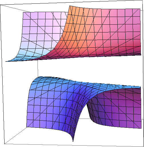
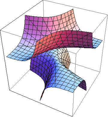
      κΦ−1​(k)\kappa_{\Phi}^{-1}(k) is a smooth surface with two connected components.

    • •

      The restriction of the projection

      κΦ−1​(k)→Πx​yℝ2\kappa_{\Phi}^{-1}(k)\xrightarrow{~\Pi_{xy}~}\mathbb{R}^{2}

      to each component is a diffeomorphism onto ℝ2\mathbb{R}^{2}.

    • •

      The components of κΦ−1​(k)\kappa_{\Phi}^{-1}(k) are graphs of functions ℝ2→z±ℝ\mathbb{R}^{2}\xrightarrow{~z_{\pm}~}\mathbb{R}.

    • •

      The sign-changes σ1,σ2\sigma_{1},\sigma_{2} permute the two components.

    • •

      When k≥2k\geq 2, the region ℝ×ℝ×[−2,2]\mathbb{R}\times\mathbb{R}\times[-2,2] separates the two components of κΦ−1​(k)\kappa_{\Phi}^{-1}(k).

  2. (2)

    κΦ−1​(−2)\kappa_{\Phi}^{-1}(-2) is connected, with one singular point (0,0,0)(0,0,0), and σ1,σ2\sigma_{1},\sigma_{2} permute the two components of κΦ−1​(−2)∖{(0,0,0)}\kappa_{\Phi}^{-1}(-2)\setminus\{(0,0,0)\}.

  3. (3)

    Finally, when k<−2k<-2, the level set κΦ−1​(k)\kappa_{\Phi}^{-1}(k) is smooth and connected. The restriction of the projection Πx​y\Pi_{xy} to κΦ−1​(k)\kappa_{\Phi}^{-1}(k) is a branched double covering of the complement of the open topological 22-disc

    {(x,y)∈ℝ2∣(x2+4)​(y2+4)<4​(2−k)}.\{(x,y)\in\mathbb{R}^{2}\mid(x^{2}+4)(y^{2}+4)<4(2-k)\}.

The only value of kk for which the level set κΦ−1​(k)\kappa_{\Phi}^{-1}(k) admits a rational parametrization is k=2k=2; compare §10 for more details. Figure 3 depicts the contours of the function (x2+4)​(y2+4)(x^{2}+4)(y^{2}+4).

4.1. Preliminaries

Let Πx​y\Pi_{xy} denote projection to the x​yxy-plane:

ℝ3\displaystyle\mathbb{R}^{3} →Πx​yℝ2\displaystyle\xrightarrow{~\Pi_{xy}~}\mathbb{R}^{2}
(20) (x,y,z)\displaystyle(x,y,z) ⟼(x,y).\displaystyle\longmapsto(x,y).

Let 𝐐z​(x,y):=x2−z​x​y+y2.\mathbf{Q}_{z}(x,y):=x^{2}-zxy+y^{2}.

Lemma 4.1.1.

For |z|<2|z|<2, the quadratic form 𝐐z\mathbf{Q}_{z} is positive definite.

Proof.

Write

(21) 𝐐z​(x,y)=2+z4​(x−y)2+2−z4​(x+y)2.\mathbf{Q}_{z}(x,y)=\frac{2+z}{4}(x-y)^{2}+\frac{2-z}{4}(x+y)^{2}.

Since |z|<2|z|<2, this is a positive linear combination of two squares. ∎

Lemma 4.1.2.

(0,0,0)(0,0,0) is the only critical point of ℝ3→κΦℝ\mathbb{R}^{3}\xrightarrow{~\kappa_{\Phi}~}\mathbb{R}.

Proof.

Since

(22) d​κΦ=(−2​x+y​z)​d​x+(−2​y+z​x)​d​y+(2​z+x​y)​d​z,d\kappa_{\Phi}=(-2x+yz)dx+(-2y+zx)dy+(2z+xy)dz,

the point p=(x,y,z)∈ℝ3p=(x,y,z)\in\mathbb{R}^{3} is critical if and only if

(23) −2​x+y​z\displaystyle-2x+yz =0\displaystyle=0
(24) −2​y+z​x\displaystyle-2y+zx =0\displaystyle=0
(25) 2​z+x​y\displaystyle 2z+xy =0.\displaystyle=0.

First suppose that z≠0z\neq 0. Then (25) implies x​y≠0xy\neq 0, that is, x≠0x\neq 0 and y≠0y\neq 0. Apply (23) and (24) to obtain:

xy=yx=z2,\frac{x}{y}=\frac{y}{x}=\frac{z}{2},

whence x/y=±1x/y=\pm 1, that is, x=±yx=\pm y and z=±2z=\pm 2. Now (25) implies x2=−4x^{2}=-4, contradicting x∈ℝx\in\mathbb{R}.

Thus z=0z=0. By (23), x=0x=0 and by (24), y=0y=0. Thus p=(0,0,0)p=(0,0,0) as desired. ∎

4.2. Projection when k>−2k>-2

The proof crucially uses:

Lemma 4.2.1.

Suppose that κΦ​(x,y,z)=k\kappa_{\Phi}(x,y,z)=k and 2​z+x​y≠02z+xy\neq 0. Then the vector fields

(26) ∂~x:=∂x+2​x−y​z2​z+x​y∂z,∂~y:=∂y+2​y−x​z2​z+x​y∂z{\widetilde{\partial}}_{x}\ :=\ \partial_{x}\ +\ \frac{2x-yz}{2z+xy}\ \partial_{z},\qquad{\widetilde{\partial}}_{y}\ :=\ \partial_{y}\ +\ \frac{2y-xz}{2z+xy}\ \partial_{z}

form a basis of the tangent space T(x,y,z)​(κΦ−1​(k))T_{(x,y,z)}\big(\kappa_{\Phi}^{-1}(k)\big). Furthermore ∂~x,∂~y{\widetilde{\partial}}_{x},\ {\widetilde{\partial}}_{y} project under d​Πx​yd\Pi_{xy} to the coordinate basis

∂x,∂y∈T(x,y)ℝ2.\partial_{x},\ \partial_{y}\in T_{(x,y)}\mathbb{R}^{2}.
Proof.

Since

(27) d​κΦ=(−2​x+y​z)​d​x+(−2​y+z​x)​d​y+(2​z+x​y)​d​z,d\kappa_{\Phi}=(-2x+yz)\ dx+(-2y+zx)\ dy+(2z+xy)\ dz,

the vector fields ∂~x,∂~y{\widetilde{\partial}}_{x},{\widetilde{\partial}}_{y} lie in the kernel of d​κΦd\kappa_{\Phi}. Therefore they are tangent to κΦ−1​(k)\kappa_{\Phi}^{-1}(k). Their projections under d​Πx​yd\Pi_{xy} form the coordinate basis of T(x,y)​ℝ2≅ℝ2T_{(x,y)}\mathbb{R}^{2}\cong\mathbb{R}^{2}. Thus they are linearly independent and base

T(x,y,z)​(κΦ−1​(k))=𝖪𝖾𝗋⁡(d​κΦ)T_{(x,y,z)}\big(\kappa_{\Phi}^{-1}(k)\big)=\mathsf{Ker}\big(d\kappa_{\Phi}\big)

as claimed. ∎

Proposition 4.2.2.

κΦ−1​(k)\kappa_{\Phi}^{-1}(k) is a smooth surface and the restriction of Πx​y\Pi_{xy} is a local diffeomorphism.

Proof.

Since κΦ​(0,0,0)=−2<k\kappa_{\Phi}(0,0,0)=-2<k, Lemma 4.1.2 implies that κΦ−1​(k)\kappa_{\Phi}^{-1}(k) contains no critical points of κΦ\kappa_{\Phi}. Thus κΦ−1​(k)⊂ℝ3\kappa_{\Phi}^{-1}(k)\subset\mathbb{R}^{3} is a smooth surface.

If 2​z+x​y≠02z+xy\neq 0, then Lemma 4.2.1 implies that Πx​y\Pi_{xy} restricts to a diffeomorphism. Thus it suffices to show 2​z+x​y≠02z+xy\neq 0.

To this end, suppose 2​z+x​y=02z+xy=0. Then κΦ​(x,y,z)=k\kappa_{\Phi}(x,y,z)=k implies:

(2​z+x​y)2=(x2+4)​(y2+4)+4​(k−2).(2z+xy)^{2}=(x^{2}+4)(y^{2}+4)+4(k-2).

Since k>−2k>-2,

0\displaystyle 0 =(2​z+x​y)2=(x2+4)​(y2+4)+4​(k−2)\displaystyle=(2z+xy)^{2}=(x^{2}+4)(y^{2}+4)+4(k-2)
≥16+4​(k−2)=4​(k+2)>0,\displaystyle\geq 16+4(k-2)=4(k+2)>0,

a contradiction. ∎

Proposition 4.2.3.

Suppose that k>−2k>-2. Then the plane ℝ×ℝ×{0}\mathbb{R}\times\mathbb{R}\times\{0\} separates κΦ−1​(k)⊂ℝ3\kappa_{\Phi}^{-1}(k)\subset\mathbb{R}^{3} into two components.

  • •

    Each component projects diffeomorphically onto ℝ2\mathbb{R}^{2} under Πx​y\Pi_{xy}.

  • •

    Each of the sign-changes σ1,σ2\sigma_{1},\sigma_{2} permutes the two components.

  • •

    When k>2k>2, the region ℝ×ℝ×[−2,2]\mathbb{R}\times\mathbb{R}\times[-2,2] separates the two components of κΦ−1​(k)⊂ℝ3\kappa_{\Phi}^{-1}(k)\subset\mathbb{R}^{3}.

  • •

    The open region ℝ×ℝ×(−2,2)\mathbb{R}\times\mathbb{R}\times(-2,2) separates the two components of κΦ−1​(2)\kappa_{\Phi}^{-1}(2).

Proof.

The identity

(28) κΦ​(x,y,z)=z2−2−𝐐z​(x,y),\kappa_{\Phi}(x,y,z)=z^{2}-2-\mathbf{Q}_{z}(x,y),

implies (since k>−2k>-2),

z2=k+2+𝐐z​(x,y)>𝐐z​(x,y).z^{2}=k+2+\mathbf{Q}_{z}(x,y)>\mathbf{Q}_{z}(x,y).

If |z|<2|z|<2, then Lemma 4.1.1 implies that 𝐐z​(x,y)≥0\mathbf{Q}_{z}(x,y)\geq 0 and z2>0z^{2}>0.

Thus z≠0z\neq 0. Consequently κΦ−1​(k)⊂ℝ3\kappa_{\Phi}^{-1}(k)\subset\mathbb{R}^{3} is the disjoint union of the two subsets where z>0z>0 and z<0z<0 respectively. These two subsets are interchanged by σi\sigma_{i}.

Suppose that k>2k>2. If |z|≤2|z|\leq 2, then, as above, Lemma 4.1.1 implies 𝐐z​(x,y)≥0\mathbf{Q}_{z}(x,y)\geq 0, and

z2=k+2+𝐐z​(x,y)≥k+2>4,z^{2}=k+2+\mathbf{Q}_{z}(x,y)\geq k+2>4,

contradicting |z|≤2|z|\leq 2. Thus ℝ×ℝ×[−2,2]\mathbb{R}\times\mathbb{R}\times[-2,2] separates the two components of κΦ−1​(k)\kappa_{\Phi}^{-1}(k). Proposition 4.2.2 implies Πx​y\Pi_{xy} restricts to a diffeomorphism, as claimed. The case k=2k=2 is handled similarly. ∎

Writing

κΦ​(x,y,z)=(z+x​y2)2−(x2+4)​(y2+4)4+2,\kappa_{\Phi}(x,y,z)=\Big(z+\frac{xy}{2}\Big)^{2}-\frac{(x^{2}+4)(y^{2}+4)}{4}+2,

the two solutions of κΦ​(x,y,z)=k\kappa_{\Phi}(x,y,z)=k are:

(29) z=z±​(x,y):=−x​y±(x2+4)​(y2+4)+4​(k−2)2.z=z_{\pm}(x,y):=\frac{-xy\pm\sqrt{(x^{2}+4)(y^{2}+4)+4(k-2)}}{2}.

Since |z|>2|z|>2, and

−x​y+(x2+4)​(y2+4)+4​(k−2)\displaystyle-xy+\sqrt{(x^{2}+4)(y^{2}+4)+4(k-2)} >0,\displaystyle>0,
−x​y−(x2+4)​(y2+4)+4​(k−2)\displaystyle-xy-\sqrt{(x^{2}+4)(y^{2}+4)+4(k-2)} <0,\displaystyle<0,

the solution z=z+​(x,y)z=z_{+}(x,y) satisfies z>2z>2 and the solution z=z−​(x,y)z=z_{-}(x,y) satisfies z<−2z<-2. Therefore κΦ−1​(k)\kappa_{\Phi}^{-1}(k) consists of two components, which are, respectively, the graphs of the functions z+,z−z_{+},z_{-} defined in (29).

Solving (28), the level set

κΦ−1​(k)∩(ℝ×ℝ×{z})\kappa_{\Phi}^{-1}(k)\cap\big(\mathbb{R}\times\mathbb{R}\times\{z\}\big)

is a (nondegenerate) hyperbola for z≠±k+2z\neq\pm\sqrt{k+2} and the union of two crossing lines (a degenerate hyperbola) for z=±k+2z=\pm\sqrt{k+2}.

First suppose that −2<k<2-2<k<2. Then

(30) (x2+4)​(y2+4)≥16>4​(2−k)(x^{2}+4)(y^{2}+4)\geq 16>4(2-k)

since k>−2k>-2.

Suppose that (x,y)∈ℝ2(x,y)\in\mathbb{R}^{2}. Then the preimages Πx​y−1​(x,y)\Pi_{xy}^{-1}(x,y) are points (x,y,z)(x,y,z) where zz is one of the two solutions z=z±​(x,y)z=z_{\pm}(x,y) given by (29). (These two solutions are distinct by (30).)

Thus

κΦ−1​(k)=𝗀𝗋𝖺𝗉𝗁⁡(z+)​∐𝗀𝗋𝖺𝗉𝗁⁡(z−)\kappa_{\Phi}^{-1}(k)=\mathsf{graph}(z_{+})\coprod\mathsf{graph}(z_{-})

and the sign-change

(31) [xyz]↦σ2[−xy−z]\begin{bmatrix}x\\ y\\ z\end{bmatrix}\xmapsto{~\sigma_{2}~}\begin{bmatrix}-x\\ y\\ -z\end{bmatrix}

interchanges these two preimages.

For −2<z<2-2<z<2, Lemma 4.1.1 implies that the quadratic form 𝐐z\mathbf{Q}_{z} is positive definite. As in the proof of Proposition 4.2.3 again, (28) expresses κΦ−1​(k)\kappa_{\Phi}^{-1}(k) as a level set of 𝐐z\mathbf{Q}_{z} for fixed zz. Thus the nonempty level sets

κΦ−1​(k)∩z−1​(z0)\kappa_{\Phi}^{-1}(k)\cap z^{-1}(z_{0})

are ellipses whenever −2<z0<2-2<z_{0}<2.

Now suppose −2<k-2<k as before. Since 2+k<2\sqrt{2+k}<2, the expression (28) of κΦ−1​(k)\kappa_{\Phi}^{-1}(k) in terms of 𝐐z\mathbf{Q}_{z} implies that κΦ−1​(k)\kappa_{\Phi}^{-1}(k) does not intersect the level set z=z0z=z_{0} when

|z0|<2+k<2.|z_{0}|<\sqrt{2+k}<2.

Thus the region ℝ×ℝ×(−2+k,2+k)\mathbb{R}\times\mathbb{R}\times\big(-\sqrt{2+k},\sqrt{2+k}\big) separates the two components of κΦ−1​(k)\kappa_{\Phi}^{-1}(k), which are interchanged by the involution σ2\sigma_{2} defined in (31).

4.3. The invariant area form

Proposition 4.2.3 implies that the coordinate functions x,yx,y give global coordinates on κΦ−1​(k)\kappa_{\Phi}^{-1}(k) when k>−2k>-2. In these coordinates the invariant area form has the following simple expression:

(32) d​Ak:=𝗌𝗂𝗀𝗇⁡(z)​d​x∧d​y(x2+4)​(y2+4)+4​(k−2)dA_{k}\ :=\ \frac{\mathsf{sign}(z)\ dx\wedge dy}{\sqrt{(x^{2}+4)(y^{2}+4)+4(k-2)}}
Lemma 4.3.1.

The exterior 22-form d​AkdA_{k} defined in (32) defines a real-analytic Γ\Gamma-invariant area form on κΦ−1​(k)\kappa_{\Phi}^{-1}(k).

Proof.

Since k>−2k>-2 and x,y∈ℝx,y\in\mathbb{R},

(x2+4)​(y2+4)+4​(k−2)≥4​(k+2)>0(x^{2}+4)(y^{2}+4)+4(k-2)\geq 4(k+2)>0

so d​AkdA_{k} is a real-analytic area form.

Since the complex exterior bivector field 𝐁\mathbf{B} on 𝖱𝖾𝗉⁡(𝖥2,𝖲𝖫⁡(2,ℂ))\mathsf{Rep}\big({\mathsf{F}}_{2},\mathsf{SL}(2,\mathbb{C})\big) defined by (16) is Γ^\widehat{\Gamma}-invariant, it suffices to show that, on the real subvariety κΦ−1​(k)\kappa_{\Phi}^{-1}(k), the complex bivector field 𝐁\mathbf{B} restricts to the real bivector field

(33) (dAk)−1:=𝗌𝗂𝗀𝗇(z)(x2+4)​(y2+4)+4​(k−2)∂x∧∂y(dA_{k})^{-1}\ :=\ \mathsf{sign}(z)\ \sqrt{(x^{2}+4)(y^{2}+4)+4(k-2)}\ \partial_{x}\wedge\partial_{y}

dual to d​AkdA_{k}. That is, we prove the embedding

ℝ2→(Πx​y)−1κΦ−1​(k)⊂ℝ3\mathbb{R}^{2}\xrightarrow{~(\Pi_{xy})^{-1}~}\kappa_{\Phi}^{-1}(k)\subset\mathbb{R}^{3}

pushes (d​Ak)−1(dA_{k})^{-1} forward to 𝐁Φ\mathbf{B}_{\Phi}.

To this end, (19) implies that d​Πx​yd\Pi_{xy} maps the Hamiltonian vector fields

𝖧𝖺𝗆⁡(x)\displaystyle\mathsf{Ham}(x) =−(2z+xy)∂y+(xz−2y)∂z\displaystyle=-(2z+xy)\ \partial_{y}+(xz-2y)\ \partial_{z} =−(2​z+x​y)​∂~y\displaystyle=-(2z+xy)\ {\widetilde{\partial}}_{y}
𝖧𝖺𝗆⁡(y)\displaystyle\mathsf{Ham}(y) =(2z+xy)∂x+(2x−yz)∂z\displaystyle=(2z+xy)\ \partial_{x}+(2x-yz)\ \partial_{z} =(2​z+x​y)​∂~x\displaystyle=(2z+xy){\widetilde{\partial}}_{x}

to −(2z+xy)∂y-(2z+xy)\ \partial_{y} and (2z+xy)∂x(2z+xy)\ \partial_{x} respectively. Now (29) implies

2​z+x​y=𝗌𝗂𝗀𝗇⁡(z)​(x2+4)​(y2+4)+4​(k−2),2z+xy=\mathsf{sign}(z)\ \sqrt{(x^{2}+4)(y^{2}+4)+4(k-2)},

completing the calculation. ∎

Similar calculations show:

(34) 𝖧𝖺𝗆⁡(z)\displaystyle\mathsf{Ham}(z) =(2y−xz)∂x+(yz−2x)∂y\displaystyle=(2y-xz)\ \partial_{x}+(yz-2x)\ \partial_{y}
=(2​y−x​z)​∂~x+(y​z−2​x)​∂~y.\displaystyle=(2y-xz)\ {\widetilde{\partial}}_{x}+(yz-2x)\ {\widetilde{\partial}}_{y}.

4.4. The level set for k≤−2k\leq-2

Here more interesting topologies arise.

Proposition 4.4.1.

Suppose that k≤−2k\leq-2.

  • •

    If k=−2k=-2, then κΦ−1​(−2)\kappa_{\Phi}^{-1}(-2) is connected, with one singular point (0,0,0)(0,0,0). Each of the two components of κΦ−1​(k)∖{(0,0,0)}\kappa_{\Phi}^{-1}(k)\setminus\{(0,0,0)\} projects diffeomorphically to ℝ2∖{(0,0)}\mathbb{R}^{2}\setminus\{(0,0)\} under Πx​y\Pi_{xy}.

  • •

    If k<−2k<-2, then κΦ−1​(k)\kappa_{\Phi}^{-1}(k) is homeomorphic to a cylinder.

Refer to caption
Figure 3. Contours of (x2+4)​(y2+4)(x^{2}+4)(y^{2}+4) on ℝ2\mathbb{R}^{2}
Proof.

When k=−2k=-2, the preimage κΦ−1​(−2)\kappa_{\Phi}^{-1}(-2) is defined by the equation

𝐐z​(x,y)=z2\mathbf{Q}_{z}(x,y)=z^{2}

which is singular only at (0,0,0)(0,0,0). The intersection κΦ−1​(−2)∖ℝ2×{0}\kappa_{\Phi}^{-1}(-2)\setminus\mathbb{R}^{2}\times\{0\} consists of two components, each being the graph of one of the functions z+,z−z_{+},z_{-} defined in (29). These two components of the complement of the origin are interchanged by σ2\sigma_{2}. This purely imaginary real form of the Markoff surface plays an important role in Bowditch’s paper [1].

Finally consider the case k<−2k<-2. In this case the image OPENΠx​y​(κΦ−1​(k)))\Pi_{xy}\big(\kappa_{\Phi}^{-1}(k))\big) is the region of ℝ2\mathbb{R}^{2} defined by

(1+(x2)2)​(1+(y2)2)≥2−k4>1.\bigg(1+\Big(\frac{x}{2}\Big)^{2}\bigg)\bigg(1+\Big(\frac{y}{2}\Big)^{2}\bigg)\geq\frac{2-k}{4}>1.

(Figure 3 depicts the level sets of this function.) For −2<z0<2-2<z_{0}<2, the ellipses defined by z=z0z=z_{0} form a cylinder. As z0→±2z_{0}\rightarrow\pm 2, their eccentricities tend to ∞\infty, and the limits (defined by z=±2z=\pm 2 are degenerate conics consisting of two parallel lines

(x∓y)2=2−k.(x\mp y)^{2}=2-k.

For |z0|>2|z_{0}|>2, the level sets are hyperbolas. The entire level set κΦ−1​(−2)\kappa_{\Phi}^{-1}(-2) is homeomorphic to a cylinder. ∎

5. Generalized Fricke spaces

Hyperbolic structures on a surface Σ\Sigma with fundamental group 𝖥2{\mathsf{F}}_{2} determine representations of 𝖥2{\mathsf{F}}_{2} into the isometry group of 𝖧2\mathsf{H}^{2}. This group identifies with the disconnected group 𝖯𝖦𝖫⁡(2,ℝ)\mathsf{PGL}(2,\mathbb{R}), and as before we lift to the double covering which we may identify with

𝖲𝖫⁡(2,ℝ)​⋃(i​𝖦𝖫​(2,ℝ)∩𝖲𝖫⁡(2,ℂ)).\mathsf{SL}(2,\mathbb{R})\bigcup\big(i\mathsf{GL}(2,\mathbb{R})\cap\mathsf{SL}(2,\mathbb{C})\big).

The homomorphism Φ\Phi is the composition

𝖥2→𝜌𝖯𝖦𝖫⁡(2,ℝ)↠π0​(𝖯𝖦𝖫⁡(2,ℝ))≅ℤ/2.{\mathsf{F}}_{2}\xrightarrow{~\rho~}\mathsf{PGL}(2,\mathbb{R})\twoheadrightarrow\pi_{0}\big(\mathsf{PGL}(2,\mathbb{R})\big)\cong\mathbb{Z}/2.

It is trivial if and only if Σ\Sigma is orientable. In that case ρ\rho preserves orientation on 𝖧2\mathsf{H}^{2}, and the lift lies in 𝖲𝖫⁡(2,ℝ)\mathsf{SL}(2,\mathbb{R}). This case is analyzed in [9]. Otherwise, exactly one of ρ⁡(X)\rho(X), ρ⁡(Y)\rho(Y) and ρ⁡(Z)\rho(Z) maps to 𝖲𝖫⁡(2,ℝ)\mathsf{SL}(2,\mathbb{R}); by applying a permutation in 𝖠𝗎𝗍⁡(𝖥2)\mathsf{Aut}({\mathsf{F}}_{2}), we may assume that ρ⁡(Z)∈𝖲𝖫⁡(2,ℝ)\rho(Z)\in\mathsf{SL}(2,\mathbb{R}), that is, Φ\Phi is the {±1}\{\pm 1\}-character with

Φ⁡(X)=Φ⁡(Y)=1​(𝗆𝗈𝖽​2),Φ⁡(Z)=0​(𝗆𝗈𝖽​2).\Phi(X)=\Phi(Y)=1\big(\mathsf{mod}~2\big),\qquad\Phi(Z)=0\big(\mathsf{mod}~2\big).

In this case, if the structure is complete, the representation is a discrete embedding, that is, an isomorphism of 𝖥2{\mathsf{F}}_{2} onto a discrete subgroup of 𝖯𝖦𝖫⁡(2,ℝ)\mathsf{PGL}(2,\mathbb{R}) and the hyperbolic surface is the quotient 𝖧2/ρ⁡(𝖥2)\mathsf{H}^{2}/\rho({\mathsf{F}}_{2}).

There are two cases for the topology of the surface 𝖧2/ρ⁡(𝖥2)\mathsf{H}^{2}/\rho({\mathsf{F}}_{2}): either it is homeomorphic to a 11-holed Klein bottle C1,1C_{1,1}, which corresponds to the case when k>2k>2, or a 22-holed cross-surface C0,2C_{0,2}, which corresponds to the case when k<2k<2. (See Charette-Drumm-Goldman [4] for more information on the Fricke space of C0,2C_{0,2}.) In the former case, we consider more general geometric structures, the boundary component of C1,1C_{1,1} is replaced by a cone point; from our viewpoint it is more natural to allow such an isolated singularity. In this particular case the singular hyperbolic surfaces behave dynamically like nonsingular complete hyperbolic structures on C1,1C_{1,1}.

Surface Σ\Sigma Peripheral elements Boundary traces
Σ0,3\Sigma_{0,3} X,Y,Z:=(X​Y)−1X,Y,Z:=(XY)^{-1} x,y,zx,y,z
Σ1,1\Sigma_{1,1} K:=X​Y​X−1​Y−1K:=XYX^{-1}Y^{-1} k:=x2+y2+z2+x​y​z−2k:=x^{2}+y^{2}+z^{2}+xyz-2
C0,2C_{0,2} Z:=X​Y,Z′:=Y−1​XZ:=XY,\quad Z^{\prime}:=Y^{-1}X z,z′:=(i​x)​(i​y)−zz,\ z^{\prime}:=(ix)(iy)-z
C1,1C_{1,1} D:=X2​Y2D:=X^{2}Y^{2} δ:=2−(i​x)2−(i​y)2+(i​x)​(i​y)​z\delta:=2-(ix)^{2}-(iy)^{2}+(ix)(iy)z

5.1. Geometric structures on the two-holed cross-surface

We begin with analyzing the Fricke space 𝔉⁡(C0,2){\mathfrak{F}}(C_{0,2}) of marked hyperbolic structures on C0,2C_{0,2} in trace coordinates. Later, in §9, we characterize the corresponding characters dynamically as those for which the flow possesses an attractor (see Definition 6.2.1, in the case when k<2k<2). Compare Goldman [12] and Charette-Drumm-Goldman [5] for further discussion.

Proposition 5.1.1.

Suppose ρ\rho is the holonomy representation for a hyperbolic structure MM on C0,2C_{0,2}. Then for some choice of basis for π1​(M)\pi_{1}(M), the character of ρ\rho satisfies

z\displaystyle z ≤−2\displaystyle\leq-2
(35) z′\displaystyle z^{\prime} =−x​y−z≤−2.\displaystyle=-xy-z\leq-2.

Conversely, if (i​x,i​y,z)(ix,iy,z) is a purely imaginary character satisfying (35), then it corresponds to a complete hyperbolic structure on C0,2C_{0,2}.

Proof.

Suppose MM is a complete hyperbolic surface diffeomorphic to C0,2C_{0,2}. Let XX be a one-sided simple curve on MM and let M|XM|X be the hyperbolic surface obtained by splitting MM along the closed geodesic corresponding to XX. Since XX is one-sided, M|XM|X is connected and has one more boundary component than MM. Furthermore χ⁡(M|X)=χ⁡(M)=−1\chi(M|X)=\chi(M)=-1 and

#​π0​(∂(M|X))=#​π0​(∂M)+1=3.\#\pi_{0}\big(\partial(M|X)\big)=\#\pi_{0}(\partial M)+1=3.

By the classification of surfaces M|X≈Σ0,3M|X\approx\Sigma_{0,3}. Thus MM is obtained from the three-holed sphere M|XM|X by attaching a cross-cap to a boundary component C⊂∂(M|X)C\subset\partial(M|X). Let A,BA,B denote the other two components of ∂(M|X)\partial(M|X), which correspond to the components of ∂M\partial M.

The Fricke space of Σ0,3\Sigma_{0,3} is parametrized by the three boundary traces (a,b,c)(a,b,c) where a=𝗍𝗋⁡(ρ⁡(A))a=\mathsf{tr}\big(\rho(A)\big), b=𝗍𝗋⁡(ρ⁡(B))b=\mathsf{tr}\big(\rho(B)\big) correspond to the boundary components of MM and CC corresponds to X−2X^{-2}. Since

OPEN𝗍𝗋⁡(ρ⁡(C))=𝗍𝗋⁡(ρ​(X)2))\displaystyle\mathsf{tr}\big(\rho(C)\big)=\mathsf{tr}\big(\rho(X)^{2})\big) =𝗍𝗋​(ρ⁡(X))2−𝗍𝗋⁡(𝕀)\displaystyle=\mathsf{tr}\big(\rho(X)\big)^{2}-\mathsf{tr}(\mathbb{I})
=−x2−2<−2,\displaystyle=-x^{2}-2\;<-2,

the other two boundary traces 𝗍𝗋⁡(ρ⁡(A))\mathsf{tr}\big(\rho(A)\big), 𝗍𝗋⁡(ρ⁡(A))\mathsf{tr}\big(\rho(A)\big) have the same sign. Applying a sign-change automorphism if necessary, we can assume they are both negative.

Let YY be another one-sided simple curve with i⁡(X,Y)=1i(X,Y)=1. Then, with appropriate choices of basepoint and representative curves, we may assume that A=X​YA=XY and B=Y−1​XB=Y^{-1}X (so that A​B​C=IABC=I). Their traces satisfy:

a+b=(i​x)​(i​y)=−x​y.a+b=(ix)(iy)=-xy.

These traces correspond to the traces z,z′z,z^{\prime} of ρ⁡(Z)=ρ⁡(Y−1​X−1)\rho(Z)=\rho(Y^{-1}X^{-1}) and ρ⁡(Z′)=ρ⁡(Y​X−1)\rho(Z^{\prime})=\rho(YX^{-1}), since

a\displaystyle a =𝗍𝗋(ρ(A))=𝗍𝗋(ρ(XY))=z,\displaystyle=\mathsf{tr}\big(\rho(A)\big)=\mathsf{tr}\big(\rho(XY)\big)\quad=z,
b\displaystyle b =𝗍𝗋⁡(ρ⁡(B))=𝗍𝗋⁡(ρ⁡(X−1​Y))=z′,\displaystyle=\mathsf{tr}\big(\rho(B)\big)=\mathsf{tr}\big(\rho(X^{-1}Y)\big)=z^{\prime},

as desired.

Conversely, suppose that (i​x,i​y,z)(ix,iy,z) is a purely imaginary character satisfying (35). Define

z′:=−z−x​y.z^{\prime}:=-z-xy.

Since

z\displaystyle z ≤−2,\displaystyle\leq-2,
z′\displaystyle z^{\prime} ≤−2,\displaystyle\leq-2,
−x2−2\displaystyle-x^{2}-2 <−2,\displaystyle<-2,

there exists a complete hyperbolic surface NN diffeomorphic to Σ0,3\Sigma_{0,3} with boundary traces (−x2−2,z,z′)(-x^{2}-2,z,z^{\prime}). The boundary components A,B,CA,B,C correspond to traces

a\displaystyle a =z,\displaystyle=z,
b\displaystyle b =z′,\displaystyle=z^{\prime},
c\displaystyle c =−x2−2.\displaystyle=-x^{2}-2.

Let MM be the complete hyperbolic surface obtained by attaching a cross-cap to CC. Then π1​(M)\pi_{1}(M) is obtained from

π1(N)=⟨A,B,C∣ABC=I⟩\pi_{1}(N)=\langle A,B,C\mid ABC=I\rangle

by adjoining a generator XX satisfying C=X−2C=X^{-2}. Define Y:=X−1​AY:=X^{-1}A, so that

X​Y\displaystyle XY =A,\displaystyle=A,
Y−1​X\displaystyle Y^{-1}X =B\displaystyle=B

and the holonomy of MM has character (i​x,i​y,z)(ix,iy,z) as desired. ∎

5.2. Geometric structures on the one-holed Klein bottle

We now determine the Fricke space and generalized Fricke space for C1,1C_{1,1} in trace coordinates. The surface C1,1C_{1,1} is rather special in that it contains a unique isotopy class of nontrivial nonperipheral 22-sided simple closed curve. We consider a marking of C1,1C_{1,1} in which this curve has homotopy class ZZ, where (X,Y,Z)(X,Y,Z) is a basic triple. Represent XX and YY by 11-sided simple loops intersecting tangentially at the basepoint (so i⁡(X,Y)=0i(X,Y)=0). With respect to a suitable choice of basepoint and defining loops, D=X2​Y2D=X^{2}Y^{2} is an element of π1​(C1,1)\pi_{1}(C_{1,1}) generating π1​(∂C1,1)\pi_{1}(\partial C_{1,1}). For a given representation ρ\rho defining a hyperbolic structure on C1,1C_{1,1}, we denote the corresponding trace function by

δ=𝗍𝗋⁡(ρ⁡(D)).\delta=\mathsf{tr}\big(\rho(D)\big).

The basic trace identity implies that

δ+k=z2.\delta+k=z^{2}.

Suppose that μ⟷(i​x,i​y,z)∈i​ℝ×i​ℝ×ℝ\mu\longleftrightarrow(ix,iy,z)\in i\mathbb{R}\times i\mathbb{R}\times\mathbb{R} is a character with k>2k>2, which corresponds to the holonomy of a hyperbolic structure on C1,1C_{1,1}. Proposition 4.2.3 implies that |z|>2|z|>2. Furthermore both x,y≠0x,y\neq 0 since otherwise 0>z2−(k+2)=𝐐z​(x,y)>00>z^{2}-(k+2)=\mathbf{Q}_{z}(x,y)>0.

Proposition 5.2.1.

Suppose that k>2k>2 and |z|<k+2|z|<\sqrt{k+2}. Let

δ:=z2−k<2.\delta:=z^{2}-k<2.

Then μ\mu corresponds to the holonomy of a hyperbolic structure on C1,1C_{1,1}

  • •

    with geodesic boundary if δ<−2\delta<-2, and the boundary has length 2cosh−1(−δ/2)2\cosh^{-1}(-\delta/2);

  • •

    with a puncture if δ=−2\delta=-2;

  • •

    with a conical singularity of cone angle cos−1(−δ/2)\cos^{-1}(-\delta/2) if −2<δ<2-2<\delta<2.

Proof.

Depending on the three cases for δ\delta, the character

(−2−x2,−2−y2,δ)(-2-x^{2},-2-y^{2},\delta)

corresponds to the holonomy of a hyperbolic surface S≈Σ0,3S\approx\Sigma_{0,3} where the boundary with trace δ\delta either is a closed geodesic, a puncture, or a conical singularity, respectively, depending on whether δ<−2\delta<-2, δ=−2\delta=-2 or 2>δ>−22>\delta>-2 respectively. Attaching a cross-cap to the boundary components corresponding to XX and YY yields a hyperbolic surface S′≈C1,1S^{\prime}\approx C_{1,1} whose holonomy has character (i​x,i​y,z)(ix,iy,z). (Compare [12] for a discussion of attaching cross-caps to geodesic boundary components of hyperbolic surfaces.) ∎

Corollary 5.2.2.

The generalized Fricke space of the one-holed Klein bottle C(1,1)C_{(1,1)} is defined by the inequalities

|z|\displaystyle|z|\quad >2\displaystyle>2
x2−z​x​y+y2\displaystyle x^{2}-zxy+y^{2}\ <0.\displaystyle<0.

Here the boundary trace δ\delta and commutator trace kk are:

δ\displaystyle\delta :=(x2−z​x​y+y2)+2\displaystyle:=\big(x^{2}-zxy+y^{2}\big)+2
k\displaystyle k :=z2−δ\displaystyle:=z^{2}-\delta

The mapping class group of C1,1C_{1,1} is realized as the subgroup of 𝖠𝗎𝗍⁡(𝖥2)\mathsf{Aut}({\mathsf{F}}_{2}) generated by the elliptic involution 𝔢\mathfrak{e}, the transposition (12)∈𝔖3(12)\in\mathfrak{S}_{3} and the involution ℑ1\mathfrak{I}_{1} defined in (6). As 𝔢\mathfrak{e} acts trivially on 𝖱𝖾𝗉⁡(𝖥2,𝖲𝖫⁡(2,ℂ))\mathsf{Rep}\big({\mathsf{F}}_{2},\mathsf{SL}(2,\mathbb{C})\big), the action on κΦ−1​(k)\kappa_{\Phi}^{-1}(k) of the subgroup of Γ\Gamma corresponding to 𝖬𝗈𝖽⁡(C1,1)\mathsf{Mod}(C_{1,1}) is generated by the transposition 𝒫(12)\mathscr{P}_{(12)} and the Vieta involutions ℑ1\mathfrak{I}_{1} and ℑ2\mathfrak{I}_{2} defined in §3.3. Figure 12 depicts these spaces.

5.3. Lines on the Markoff surface

Here we interpret lines on the imaginary real form on the Markoff surface (k=−2k=-2) as Fricke spaces of a certain 22-orbifold. Lee and Sakuma [16, 17] studied the complex lines on the Markoff surface. We consider the real lines on the real form and show they contain characters of non-injective representations with discrete image and identify the quotient hyperbolic orbifold.

Recall that the Markoff surface is defined by (ξ,η,ζ)∈ℂ3(\xi,\eta,\zeta)\in\mathbb{C}^{3} satisfying ξ2+η2+ζ2=ξ​η​ζ\xi^{2}+\eta^{2}+\zeta^{2}=\xi\eta\zeta. We consider the lines defined by the vanishing of one of the coordinates, for example ξ=0\xi=0. In that case the lines are defined by ζ=±i​η\zeta=\pm i\eta, which yield imaginary characters (0,i​y,y)(0,iy,y), where y∈ℝy\in\mathbb{R}. We show that, when y≥2y\geq 2, these correspond to representations of 𝖥2{\mathsf{F}}_{2} with discrete image.

Write (ξ,η,ζ)=(0,2​i​sinh⁡(ℓ/2),sinh⁡(ℓ/2))(\xi,\eta,\zeta)=\big(0,2i\sinh(\ell/2),\sinh(\ell/2)\big), so that YY corresponds to a glide-reflection of displacement ℓ\ell, or a reflection when ℓ=0\ell=0. Representative matrices are, for example:

ρ⁡(X)\displaystyle\rho(X) =i​[−1001],\displaystyle=i\begin{bmatrix}-1&0\\ 0&1\end{bmatrix},
ρ⁡(Y)\displaystyle\rho(Y) =i​[2​sinh⁡(ℓ/2)110],\displaystyle=i\begin{bmatrix}2\sinh(\ell/2)&1\\ 1&0\end{bmatrix},
ρ⁡(Z)\displaystyle\rho(Z) =[0−1−12​sinh⁡(ℓ/2)]\displaystyle=\begin{bmatrix}0&-1\\ -1&2\sinh(\ell/2)\end{bmatrix}

Then ρ⁡(X)\rho(X) represents the reflection and ρ⁡(Y)\rho(Y) represents a glide-reflection (or reflection when ℓ=0\ell=0), whose respective fixed-point sets are:

𝖥𝗂𝗑⁡(ρ⁡(X))\displaystyle\mathsf{Fix}\big(\rho(X)\big) ={0,∞}\displaystyle=\{0,\infty\}
𝖥𝗂𝗑⁡(ρ⁡(Y))\displaystyle\mathsf{Fix}\big(\rho(Y)\big) ={eℓ/2,−e−ℓ/2}\displaystyle=\{e^{\ell/2},-e^{-\ell/2}\}

If ℓ>2​log⁡(1+2)\ell>2\log(1+\sqrt{2}), then ρ⁡(Z)\rho(Z) is a transvection with

𝖥𝗂𝗑⁡(ρ⁡(Z))={−sinh⁡(ℓ/2)±cosh2⁡(ℓ)−3/2}.\mathsf{Fix}\big(\rho(Z)\big)=\Big\{-\sinh(\ell/2)\pm\sqrt{\cosh^{2}(\ell)-3/2}\Big\}.

When ℓ=2​log⁡(1+2)\ell=2\log(1+\sqrt{2}), then ρ⁡(Z)\rho(Z) is a parabolic fixing −1-1.

In these latter two cases, 𝖨𝗆𝖺𝗀𝖾⁡(ρ)\mathsf{Image}(\rho) is discrete, and the quotient hyperbolic orbifold 𝖧2/𝖨𝗆𝖺𝗀𝖾⁡(ρ)\mathsf{H}^{2}/\mathsf{Image}(\rho) is a punctured disc with a mirrored arc on its boundary. Its orbifold double covering-space

𝖧2/⟨ρ⁡(Y),ρ⁡(X)​ρ​(Y)​ρ​(X)⟩\mathsf{H}^{2}/\langle\rho(Y),\,\rho(X)\rho(Y)\rho(X)\rangle

is a two-holed cross-surface C0,2C_{0,2} with reflection symmetry defined by the reflection ρ⁡(X)\rho(X). When ℓ=2​log⁡(1+2)\ell=2\log(1+\sqrt{2}), the corresponding character is (2​i,2​i,2)(2i,2i,2). The closed ray defined by ℓ≥2​log⁡(1+2)\ell\geq 2\log(1+\sqrt{2}) corresponds to the Fricke space of this nonorientable hyperbolic orbifold 𝖧2/𝖨𝗆𝖺𝗀𝖾⁡(ρ)\mathsf{H}^{2}/\mathsf{Image}(\rho).

6. Bowditch theory

Bowditch [1] introduced objects (which he called Markoff maps)

Ω→𝜇ℂ\Omega\xrightarrow{~\mu~}\mathbb{C}

which are equivalent to characters in 𝖱𝖾𝗉⁡(𝖥2,𝖲𝖫⁡(2,ℂ))≅ℂ3\mathsf{Rep}\big({\mathsf{F}}_{2},\mathsf{SL}(2,\mathbb{C})\big)\cong\mathbb{C}^{3} where the commutator of a pair of free generators has trace −2-2. (Tan-Wong-Zhang [29] extended this to arbitrary characters in 𝖱𝖾𝗉⁡(𝖥2,𝖲𝖫⁡(2,ℂ))≅ℂ3\mathsf{Rep}\big({\mathsf{F}}_{2},\mathsf{SL}(2,\mathbb{C})\big)\cong\mathbb{C}^{3}, calling them generalized Markoff maps.) Bowditch used Markoff maps to study the orbit of a character under the action of the automorphism group 𝖠𝗎𝗍⁡(𝖥2)\mathsf{Aut}({\mathsf{F}}_{2}). Departing from Bowditch’s terminology, we call these maps trace labelings. We apply Bowditch’s approach to the dynamics of the Γ\Gamma-action on purely imaginary characters

(ξ,η,ζ)∈i​ℝ×i​ℝ×ℝ⊂ℂ3.(\xi,\eta,\zeta)\in i\mathbb{R}\times i\mathbb{R}\times\mathbb{R}\subset\mathbb{C}^{3}.

This section reviews the theory in the more general setting of 𝖲𝖫⁡(2,ℂ)\mathsf{SL}(2,\mathbb{C})-characters, that is, when (ξ,η,ζ)⊂ℂ3(\xi,\eta,\zeta)\subset\mathbb{C}^{3} before specializing to the purely imaginary characters.

Bowditch’s method was used and extended by Tan, Wong and Zhang in [27, 26, 28] and Maloni-Palesi-Tan [19] to study various aspects of the dynamics of this action, and obtain variations of McShane’s identities. See the above papers for more details.

Following Bowditch [1], encode the dynamics of the action of 𝖮𝗎𝗍⁡(𝖥2)\mathsf{Out}({\mathsf{F}}_{2}) on characters, described by trace labelings μ∈𝖱𝖾𝗉⁡(𝖥2,𝖲𝖫⁡(2,ℂ))\mu\in\mathsf{Rep}({\mathsf{F}}_{2},\mathsf{SL}(2,\mathbb{C})), in terms of a dynamical system on the tree 𝖳\mathsf{T}. The character provides a way of directing 𝖳\mathsf{T}, and the dynamics of the associated directed tree 𝖳→μ\overrightarrow{\mathsf{T}}_{\mu} (the flow) is Bowditch’s invariant.

6.1. The trace labeling associated to a character

Suppose that

𝖥2→𝜌𝖲𝖫⁡(2,ℂ){\mathsf{F}}_{2}\xrightarrow{~\rho~}\mathsf{SL}(2,\mathbb{C})

is a representation. Define the corresponding trace labeling μρ\mu_{\rho}:

Ω\displaystyle\Omega →μρℂ\displaystyle\xrightarrow{~\mu_{\rho}~}\mathbb{C}
ω\displaystyle\omega ⟼𝗍𝗋⁡(ρ⁡(γω))\displaystyle\longmapsto\mathsf{tr}\big(\rho(\gamma_{\omega})\big)

where γω\gamma_{\omega} is an element of 𝖥2{\mathsf{F}}_{2} corresponding to ω\omega. The trace labeling μ\mu associated to a character in 𝖱𝖾𝗉⁡(𝖥2,𝖲𝖫⁡(2,ℂ))≅ℂ3\mathsf{Rep}\big({\mathsf{F}}_{2},\mathsf{SL}(2,\mathbb{C})\big)\cong\mathbb{C}^{3} satisfies a equation for each edge and an equation for each vertex as follows.

First, fix the parameter

k=κ⁡(μ):=κ⁡(ξ,η,ζ)k=\kappa(\mu):=\kappa(\xi,\eta,\zeta)

throughout the discussion. Vertex Relation (37) implies that κ\kappa is constant on vertices of 𝖳\mathsf{T} and Edge Relation (36) provides the basic inductive step for navigating through 𝖳\mathsf{T}. In particular, once μ\mu is defined on the three regions around a vertex, then (36) forces a unique extension Ω→ℂ\Omega\to\mathbb{C}.

Suppose that eX,Y​(Z,Z′)∈𝖤𝖽𝗀𝖾⁡(𝖳)e^{X,Y}(Z,Z^{\prime})\in\mathsf{Edge}(\mathsf{T}) is an edge. Then

(36) ζ+ζ′=ξ​η\zeta+\zeta^{\prime}=\xi\eta

Suppose v=v⁡(X,Y,Z)∈𝖵𝖾𝗋𝗍⁡(𝖳)v=v(X,Y,Z)\in\mathsf{Vert}(\mathsf{T}) is a vertex. Then

(37) ξ2+η2+ζ2−ξ​η​ζ−2=k\xi^{2}+\eta^{2}+\zeta^{2}-\xi\eta\zeta-2\;=\;k

where the lower case Greek letters represent the trace labeling of the region denoted by the corresponding upper case Roman letters. Figure 4 depicts an example of a trace labeling.

The Edge Relation (36) and the Vertex Relation (37) intimately relate. Fixing a pair X,Y∈ΩX,Y\in\Omega which abut one another, there are exactly two elements of Ω\Omega which abut XX and YY; these are ZZ and Z′Z^{\prime} respectively. Their corresponding traces ζ,ζ′\zeta,\zeta^{\prime} are the two roots of the quadratic equation obtained from (37) by fixing ξ,η\xi,\eta. This follows directly from (36).

The trace labeling μ\mu also intimately relates to the Γ\Gamma-action on the character variety 𝖱𝖾𝗉⁡(𝖥2,𝖲𝖫⁡(2,ℂ))\mathsf{Rep}\big({\mathsf{F}}_{2},\mathsf{SL}(2,\mathbb{C})\big). In particular, the triple of trace values about each vertex is the image of μ\mu under an element of Γ\Gamma. This is the action of Γ\Gamma on superbases described in (9) where the superbasis determines a coordinate system 𝖱𝖾𝗉⁡(𝖥2,𝖲𝖫⁡(2,ℂ))≅ℂ3\mathsf{Rep}\big({\mathsf{F}}_{2},\mathsf{SL}(2,\mathbb{C})\big)\cong\mathbb{C}^{3}.

Conversely, for any γ∈Γ\gamma\in\Gamma, the image γ⁡(μ)\gamma(\mu) is a triple of trace values around some vertex of the tree.

Refer to caption
Figure 4. Labeling the trivalent tree by traces

6.2. The flow associated to a character

From the trace labeling μ\mu associated to a character in 𝖱𝖾𝗉⁡(𝖥2,𝖲𝖫⁡(2,ℂ))\mathsf{Rep}({\mathsf{F}}_{2},\mathsf{SL}(2,\mathbb{C})), Bowditch [1] associates a directed tree 𝖳→\overrightarrow{\mathsf{T}} (which Tan-Wong-Zhang [29] call a flow on 𝖳\mathsf{T}) as follows.

Suppose that

e=eX,Y​(Z,Z′)∈𝖤𝖽𝗀𝖾⁡(𝖳)e=e^{X,Y}(Z,Z^{\prime})\in\mathsf{Edge}(\mathsf{T})

is an edge. Say that ee is decisive (relative to μ\mu) if

|ζ|≠|ζ′|;|\zeta|\neq|\zeta^{\prime}|;

in that case direct the edge as follows:

{eX,Y​(Z→Z′):⟺|ζ|>|ζ′|eX,Y​(Z←Z′):⟺|ζ|<|ζ′|.\begin{cases}e^{X,Y}(Z\rightarrow Z^{\prime})&:\Longleftrightarrow|\zeta|>|\zeta^{\prime}|\\ e^{X,Y}(Z\leftarrow Z^{\prime})&:\Longleftrightarrow|\zeta|<|\zeta^{\prime}|.\end{cases}

Otherwise, say that ee is indecisive and assign either direction to the edge ee. Say that an edge ee points decisively towards a vertex vv if and only if ee is decisive and points towards vv.

If every edge is decisive, say that μ\mu is completely decisive. If every edge is indecisive, say that μ\mu is completely indecisive. For many cases of interest, only finitely many edges are indecisive. The ambiguity at an indecisive edge does not affect the subsequent discussion. In particular, if the arrow points from ZZ to Z′Z^{\prime}, then |ζ|≥|ζ′||\zeta|\geq|\zeta^{\prime}|. Denote the above directed tree by 𝖳→(ξ,η,ζ)\overrightarrow{\mathsf{T}}_{(\xi,\eta,\zeta)} or 𝖳→μ\overrightarrow{\mathsf{T}}_{\mu}.

Sign-change automorphisms do not affect the directed tree 𝖳→μ\overrightarrow{\mathsf{T}}_{\mu} associated to a character μ\mu.

The vertices 𝖵𝖾𝗋𝗍⁡(𝖳→)\mathsf{Vert}(\overrightarrow{\mathsf{T}}) admit the following classification:

Number of edges pointing towards vv Type of vv
0 source
1 fork
2 merge
3 sink
(a)
(b)
(c)
(d)
Figure 5. Types of vertices in a directed tree

Each merge possesses a unique trace-reducing direction since exactly one directed edge incident to vv points away from vv.

The following definition is due to Tan-Wong-Zhang [29], §2.18 and is a crucial idea in Bowditch [1]:

Definition 6.2.1.

Let 𝖳→\overrightarrow{\mathsf{T}} be a directed tree. An attractor in 𝖳→\overrightarrow{\mathsf{T}} is a minimal subtree 𝖠→⊂𝖳→\vec{\mathsf{A}}\subset\overrightarrow{\mathsf{T}} satisfying the following two properties:

  • •

    𝖠→\vec{\mathsf{A}} is finite;

  • •

    Every edge e∉𝖠→e\notin\vec{\mathsf{A}} points inward towards 𝖠→\vec{\mathsf{A}}.

Examples of attractors include sinks and attracting indecisive edges. For imaginary characters, these are the only types of attractors.

Proposition 6.2.2.

Γ\Gamma acts properly on the set 𝒮\mathscr{S} of characters μ\mu for which 𝖳→μ\overrightarrow{\mathsf{T}}_{\mu} has an attractor.

Proof.

Denote by 𝖥𝗂𝗇𝗂𝗍𝖾⁡(𝖵𝖾𝗋𝗍⁡(𝖳))\mathsf{Finite}\big(\mathsf{Vert}(\mathsf{T})\big) the set of finite subsets of 𝖵𝖾𝗋𝗍⁡(𝖳)\mathsf{Vert}(\mathsf{T}). Then the map

𝒮⟶𝖥𝗂𝗇𝗂𝗍𝖾⁡(𝖵𝖾𝗋𝗍⁡(𝖳))\mathscr{S}\longrightarrow\mathsf{Finite}\big(\mathsf{Vert}(\mathsf{T})\big)

which associates to μ∈𝒮\mu\in\mathscr{S} the attractor of 𝖳→μ\overrightarrow{\mathsf{T}}_{\mu} is Γ\Gamma-equivariant. Since Γ\Gamma acts properly on 𝖥𝗂𝗇𝗂𝗍𝖾⁡(𝖵𝖾𝗋𝗍⁡(𝖳))\mathsf{Finite}\big(\mathsf{Vert}(\mathsf{T})\big), it acts properly on 𝒮\mathscr{S}. ∎

Definition 6.2.3.

A descending path in the directed tree 𝖳→μ\vec{\mathsf{T}}_{\mu} is a path in 𝖳\mathsf{T} as above, where each edge fif_{i} points away from viv_{i} and towards vi+1v_{i+1}:

(38) P→=(u0→f0u1→f1⋯→fn−1un→fn⋯)\vec{P}=\big(u_{0}\xrightarrow{f_{0}}u_{1}\xrightarrow{f_{1}}\cdots\xrightarrow{f_{n-1}}u_{n}\xrightarrow{f_{n}}\cdots\big)

where ui∈𝖵𝖾𝗋𝗍⁡(𝖳)u_{i}\in\mathsf{Vert}(\mathsf{T}) and fi∈𝖤𝖽𝗀𝖾⁡(𝖳)f_{i}\in\mathsf{Edge}(\mathsf{T}), which forms a geodesic in 𝖳\mathsf{T}.

If PP is a descending path as above, then the sequence of values (ξn,ηn,ζn)(\xi_{n},\eta_{n},\zeta_{n}) at unu_{n} are decreasing in absolute value, that is:

|ξn+1|\displaystyle|\xi_{n+1}| ≤|ξn|\displaystyle\leq|\xi_{n}|
|ηn+1|\displaystyle|\eta_{n+1}| ≤|ηn|\displaystyle\leq|\eta_{n}|
(39) |ζn+1|\displaystyle|\zeta_{n+1}| ≤|ζn|.\displaystyle\leq|\zeta_{n}|.

This follows since at each step, two of the three coordinates ξ,η,ζ\xi,\eta,\zeta remain constant and the absolute value of the remaining coordinate does not increase.

Figure 6. The regions around an alternating geodesic

6.3. Exceptional characters

We state here some of the basic results associated to the trace labelings μ\mu as well as the directed trees 𝖳→μ\vec{\mathsf{T}}_{\mu}; see [1], [28],and [29] for more details. For ease of exposition, we exclude certain exceptional cases from our discussion below.

To begin, exclude the characters arising from reducible representations, namely characters in κ−1​(2)\kappa^{-1}(2). The dynamics on the set of reducible characters is discussed in [12]. Next, exclude the Γ^\widehat{\Gamma}-orbit

Γ^⋅({0}×ℂ×ℂ).\widehat{\Gamma}\cdot\big(\{0\}\times\mathbb{C}\times\mathbb{C}\big).

For each k∈ℂk\in\mathbb{C}, this set intersects κ−1​(k)\kappa^{-1}(k) in a set of measure zero, and hence does not affect our claims of ergodicity. Nonetheless this case presents quite interesting dynamics.

Among the exceptional characters are dihedral characters. These are characters of representations where both elements of some basis map to involutions in 𝖲𝖫⁡(2,ℂ)\mathsf{SL}(2,\mathbb{C}). Taking that basis to be (X,Y)(X,Y), the corresponding character equals (0,0,ζ)(0,0,\zeta) for some ζ∈ℂ\zeta\in\mathbb{C}. Therefore dihedral characters lie in the Γ\Gamma-orbit of the coordinate line {0}×{0}×ℂ\{0\}\times\{0\}\times\mathbb{C}. The orbit of (0,0,ζ)(0,0,\zeta) equals

{(0,0,ζ),(0,0,−ζ),(0,ζ,0),(0,−ζ,0),(ζ,0,0),(−ζ,0,0)}.\big\{(0,0,\zeta),(0,0,-\zeta),(0,\zeta,0),(0,-\zeta,0),(\zeta,0,0),(-\zeta,0,0)\big\}.

Dihedral characters are the most degenerate characters since directing the tree 𝖳\mathsf{T} is completely arbitrary: The directed trees corresponding to dihedral characters are completely indecisive.

We call the elements of the set

κ−1​(2)∪(Γ^⋅(0,η,ζ))⊂ℂ3\kappa^{-1}(2)\ \cup\ (\widehat{\Gamma}\cdot(0,\eta,\zeta))\ \subset\ \mathbb{C}^{3}

exceptional characters, and elements of its complement unexceptional characters. The associated trace labelings and directed trees are called exceptional or unexceptional accordingly. Note that an unexceptional trace labeling μ\mu takes values only in ℂ∖{0}\mathbb{C}\setminus\{0\}.

6.4. The Fork Lemma

The following fundamental result is proved in [1] (Lemma 3.2(3)) for characters (ξ,η,ζ)∈κ−1​(−2)(\xi,\eta,\zeta)\in\kappa^{-1}(-2) and extended in [29] (Lemma 3.7) and [28] (Proposition 3.3) for general characters. Recall that if the two edges are directed away from a vertex vv, then that vertex must either be a fork or a source. We will see that such vertices are rare in our applications.

We supply a brief proof for the reader’s convenience.

Lemma 6.4.1 (The Fork Lemma).

Suppose that μ\mu is a trace labeling with directed tree 𝖳→μ\vec{\mathsf{T}}_{\mu}. If for the vertex v⁡(X,Y,Z)∈𝖵𝖾𝗋𝗍⁡(𝖳)v(X,Y,Z)\in\mathsf{Vert}(\mathsf{T}), the edges opposite to XX and YY are directed away from XX and YY respectively, then |ζ|≤2|\zeta|\leq 2 or ξ=η=0\xi=\eta=0.

Proof.

Write eY,Z​(X→X′)e^{Y,Z}(X\rightarrow X^{\prime}) and eX,Z​(Y→Y′)e^{X,Z}(Y\rightarrow Y^{\prime}) for the two edges directed away from vv, with corresponding traces ξ,η,ζ,ξ′,η′\xi,\eta,\zeta,\xi^{\prime},\eta^{\prime}. By assumption,

|ξ|\displaystyle|\xi| ≥|ξ′|\displaystyle\geq|\xi^{\prime}|
|η|\displaystyle|\eta| ≥|η′|,\displaystyle\geq|\eta^{\prime}|,

which implies:

2​|ξ|≥|ξ|+|ξ′|\displaystyle 2|\xi|\geq|\xi|+|\xi^{\prime}| ≥|ξ+ξ′|=|η​ζ|\displaystyle\geq|\xi+\xi^{\prime}|=|\eta\zeta|
2​|η|≥|η|+|η′|\displaystyle 2|\eta|\geq|\eta|+|\eta^{\prime}| ≥|η+η′|=|ξ​ζ|\displaystyle\geq|\eta+\eta^{\prime}|=|\xi\zeta|

Summing these two equations yields:

2​(|ξ|+|η|)≥|ζ|​(|ξ|+|η|)2\ \big(|\xi|+|\eta|\big)\;\geq\;|\zeta|\ \big(|\xi|+|\eta|\big)

Thus 2≥|ζ|2\geq|\zeta| or ξ=η=0\xi=\eta=0. ∎

Since characters vanishing on a pair of two adjacent complementary regions are exceptional, a region YY adjacent to a source or a fork arising from an unexceptional character must satisfy |μ⁡(Y)|≤2|\mu(Y)|\leq 2.

We prove properness of the action using the two Q-conditions introduced by Bowditch in [1]. These conditions describe an open subset of the relative character variety with proper Γ\Gamma-action. Tan-Wong-Zhang [29] extended this set to an open subset of the full character variety with proper Γ\Gamma-action. For our purposes, we relax the conditions slightly, allowing finitely many parabolics among the set of primitive elements as in [27]. The resulting subset is no longer open, but the Γ\Gamma-action remains proper.

Definition 6.4.2.

Given a character μ\mu and constant C>0C>0, define Ωμ​(C)\Omega_{\mu}(C) to be the union of the set of closures of complementary regions Y∈ΩY\in\Omega with |μ⁡(Y)|≤C|\mu(Y)|\leq C.

Lemma 6.4.1 immediately implies:

Lemma 6.4.3 (Bowditch [1], Theorem 1(2))).

Suppose C≥2C\geq 2. For every character μ\mu, the set Ωμ​(C)\Omega_{\mu}(C) is connected.

(See also [29], Theorem 3.1(2).)

The following (extended) BQ-conditions were first defined by Bowditch in [1], and generalized by Tan-Wong-Zhang [29, 27]):

(40) μ⁡(X)\displaystyle\mu(X) ∉[−2,2]​ for all ​X∈Ω;\displaystyle\not\in[-2,2]\text{~for all~}X\in\Omega;
(41) μ⁡(X)\displaystyle\mu(X) ∉(−2,2)​ for all ​X∈Ω;\displaystyle\not\in(-2,2)\text{~for all~}X\in\Omega;
(42) Ωμ​(2)\displaystyle\Omega_{\mu}(2) ={Y∈Ω:|μ⁡(Y)|≤2}​ is finite.\displaystyle=\{Y\in\Omega:|\mu(Y)|\leq 2\}\text{~is finite.}

Condition (40) means that every primitive element of 𝖥2{\mathsf{F}}_{2} maps to a loxodromic element, and Condition (41) means that no primitive element of 𝖥2{\mathsf{F}}_{2} maps to an elliptic. Condition (42) is equivalent to the condition that Ωμ​(C)\Omega_{\mu}(C) is finite for any C≥2C\geq 2. See [1] and [27] for details.

Definition 6.4.4.

A character μ\mu is a Bowditch character if and only if μ\mu is irreducible and satisfies (40) and (42) above. A character μ\mu is an extended Bowditch character if and only if μ\mu is unexceptional and irreducible and satisfies (41) and (42) above.

The Bowditch set 𝔅\mathfrak{B} comprises all Bowditch characters, and the extended Bowditch set 𝔅′\mathfrak{B}^{\prime} comprises all extended Bowditch characters.

Condition (41) allows for finitely many such parabolics among the primitives. The extended Bowditch set 𝔅′\mathfrak{B}^{\prime} is no longer open in ℂ3\mathbb{C}^{3} but Γ\Gamma still acts properly on it.

Exceptional characters do not lie in 𝔅\mathfrak{B}: in the case of the reducible characters where k=2k=2 by definition and otherwise, Condition (40) is not satisfied if

μ∈Γ^⋅(0,η,ζ).\mu\in\widehat{\Gamma}\cdot(0,\eta,\zeta).

Similarly, if

μ⁡(Z)=±k+2\mu(Z)=\pm\sqrt{k+2}

for some Z∈ΩZ\in\Omega, then the proof of Proposition 6.5.4 implies that μ\mu cannot satisfy Condition (42).

Bowditch [1] and Tan-Wong-Zhang [29, 27] proved that 𝔅\mathfrak{B} is an open subset of the character variety and, for every μ∈𝔅′\mu\in\mathfrak{B}^{\prime}, the flow 𝖳→μ\overrightarrow{\mathsf{T}}_{\mu} possesses an attractor. Thus Proposition 6.2.2 implies:

Theorem 6.4.5 ( Bowditch [1], Tan-Wong-Zhang [29]).

Γ\Gamma acts properly on the extended Bowditch set 𝔅′\mathfrak{B}^{\prime}.

For general μ∈𝖱𝖾𝗉⁡(𝖥2,𝖲𝖫⁡(2,ℂ))\mu\in\mathsf{Rep}\big({\mathsf{F}}_{2},\mathsf{SL}(2,\mathbb{C})\big), Tan-Wong-Zhang [28] associate a closed subset ℰ⁡(μ)\mathcal{E}(\mu) of the projectivized measured lamination space of Σ1,1\Sigma_{1,1}, the set of end invariants of μ\mu. (This space identifies with 𝖯1​(ℝ)\mathsf{P}^{1}(\mathbb{R}), the completion of 𝖯1​(ℚ)\mathsf{P}^{1}(\mathbb{Q}). A character μ\mu lies in 𝔅′\mathfrak{B}^{\prime} if and only if ℰ⁡(μ)=∅\mathcal{E}(\mu)=\emptyset ([28], Theorem 1.3). We complete their computation of ℰ⁡(μ)\mathcal{E}(\mu) for imaginary characters in this paper. We show that, for k>2k>2, either ℰ⁡(μ)=∅\mathcal{E}(\mu)=\emptyset (when μ\mu lies in the domain of discontinuity of the Γ\Gamma-action) or ℰ⁡(μ)\mathcal{E}(\mu) consists of only one point.

6.5. Alternating geodesics

For a fixed Z∈ΩZ\in\Omega, the values of a trace labeling μ\mu on the other regions abutting C⁡(Z)C(Z) admits an explicit description by inductively iterating (36).

First we establish some notation. Choose a trace labeling μ\mu associated to a character [ρ]∈𝖱𝖾𝗉⁡(𝖥2,𝖲𝖫⁡(2,ℂ))[\rho]\in\mathsf{Rep}\big({\mathsf{F}}_{2},\mathsf{SL}(2,\mathbb{C})\big). Denote the trace μ⁡(A)\mu(A) associated with A∈ΩA\in\Omega by the corresponding lower-case letter aa.

Let {vn∣n∈ℤ}\{v_{n}\mid n\in\mathbb{Z}\} be the ordered set of vertices adjacent to ZZ, labeled so that

vn=v⁡(Yn−1,Yn,Z),v_{n}=v(Y_{n-1},Y_{n},Z),

inductively beginning at Y0=XY_{0}=X and Y1=YY_{1}=Y. Let en∈𝖤𝖽𝗀𝖾⁡(𝖳)e_{n}\in\mathsf{Edge}(\mathsf{T}) be the edge between vnv_{n} and vn+1v_{n+1}. We write

⋯ e−1v0 e0v1 e1v2 e2⋯\cdots\stackrel{{\scriptstyle e_{-1}}}{{\rule[3.61371pt]{14.45377pt}{0.72229pt}}}v_{0}\stackrel{{\scriptstyle e_{0}}}{{\rule[3.61371pt]{14.45377pt}{0.72229pt}}}v_{1}\stackrel{{\scriptstyle e_{1}}}{{\rule[3.61371pt]{14.45377pt}{0.72229pt}}}v_{2}\stackrel{{\scriptstyle e_{2}}}{{\rule[3.61371pt]{14.45377pt}{0.72229pt}}}\cdots

for this geodesic. Let Yn∈ΩY_{n}\in\Omega be the region adjacent to ZZ sharing the edge ene_{n} with ZZ. Finally, let ψn\psi_{n} be the edge incident to vnv_{n} not adjacent to ZZ, and Zn′∈ΩZ_{n}^{\prime}\in\Omega the other region opposite to the edge ψn\psi_{n}. Denote the corresponding traces by ζ=μ⁡(Z)\zeta=\mu(Z) and ηn=μ⁡(Yn)\eta_{n}=\mu(Y_{n}). Compare Figure 6.

The indices j⁡(en)∈{1,2,3}j(e_{n})\in\{1,2,3\} for the tricoloring described in §2.3 alternate between two elements in {1,2,3}\{1,2,3\}, depending on the mod 22 class associated to ZZ. This leads to a simple formula (43) for the set of traces ηn\eta_{n}. In particular the sequence of characters forms a lattice in a hyperbola. Recall that the hyperbola {(ξ,η)∣ξ​η=1}\{(\xi,\eta)\mid\xi\eta=1\} is naturally an algebraic group (the multiplicative group of the ground field), and a lattice is a discrete subgroup Λ\Lambda with compact quotient; such a lattice is necessarily a cyclic group.

Proposition 6.5.1.

Suppose ζ≠±2\zeta\neq\pm 2. Let λ,λ−1\lambda,\lambda^{-1} be the two (distinct) solutions of

λ2−ζ​λ+1=0\lambda^{2}-\zeta\lambda+1=0

so that

ζ=λ+λ−1.\zeta=\lambda+\lambda^{-1}.

Then, for n∈ℤn\in\mathbb{Z},

(43) ηn=A​λn+B​λ−n\eta_{n}\ =\;A\lambda^{n}\ +\ B\lambda^{-n}

where

A\displaystyle A =η−λ−1​ξλ−λ−1\displaystyle=\frac{\eta-\lambda^{-1}\xi}{\lambda-\lambda^{-1}}
B\displaystyle B =λ​ξ−ηλ−λ−1.\displaystyle=\frac{\lambda\xi-\eta}{\lambda-\lambda^{-1}}.

Furthermore

A​B=ζ2−k−2ζ2−4.AB=\frac{\zeta^{2}-k-2}{\zeta^{2}-4}.
Proof.

(36) implies that ηn\eta_{n} satisfies the recursion

ηn+1=ζ​ηn+ηn−1.\eta_{n+1}=\zeta\eta_{n}+\eta_{n-1}.

Rewrite this recursion as:

𝐘n+1=𝐙𝐘n\mathbf{Y}_{n+1}=\mathbf{Z}\mathbf{Y}_{n}

in terms of a vector variable 𝐘n\mathbf{Y}_{n} and matrix variable 𝐙\mathbf{Z} defined by:

𝐘n:=[ηnηn−1],𝐙=[ζ−110].\mathbf{Y}_{n}:=\begin{bmatrix}\eta_{n}\\ \eta_{n-1}\end{bmatrix},\ \mathbf{Z}=\begin{bmatrix}\zeta&-1\\ 1&0\end{bmatrix}.

Diagonalize 𝐙\mathbf{Z} as:

𝐙=1λ−λ−1​[λ−1λ11]​[λ−100λ]​[−1λ1−λ−1]\mathbf{Z}=\frac{1}{\lambda-\lambda^{-1}}\begin{bmatrix}\lambda^{-1}&\lambda\\ 1&1\end{bmatrix}\begin{bmatrix}\lambda^{-1}&0\\ 0&\lambda\end{bmatrix}\begin{bmatrix}-1&\lambda\\ 1&-\lambda^{-1}\end{bmatrix}

where

1λ−λ−1​[λ−1λ11]​[−1λ1−λ−1]=[1001].\frac{1}{\lambda-\lambda^{-1}}\begin{bmatrix}\lambda^{-1}&\lambda\\ 1&1\end{bmatrix}\begin{bmatrix}-1&\lambda\\ 1&-\lambda^{-1}\end{bmatrix}=\begin{bmatrix}1&0\\ 0&1\end{bmatrix}.

Then

𝐘n=𝐙n​𝐘0=1λ−λ−1​[λ−1λ11]​[λ−n00λn]​[−1λ1−λ−1]\mathbf{Y}_{n}=\mathbf{Z}^{n}\mathbf{Y}_{0}=\frac{1}{\lambda-\lambda^{-1}}\begin{bmatrix}\lambda^{-1}&\lambda\\ 1&1\end{bmatrix}\begin{bmatrix}\lambda^{-n}&0\\ 0&\lambda^{n}\end{bmatrix}\begin{bmatrix}-1&\lambda\\ 1&-\lambda^{-1}\end{bmatrix}

from which the result follows. ∎

When ζ=±2\zeta=\pm 2, the situation is even simpler:

Proposition 6.5.2.

If ζ=2\zeta=2, then

ηn=ξ+n⁡(η−ξ)\eta_{n}=\xi+n(\eta-\xi)

and if ζ=−2\zeta=-2, then

ηn=(−1)n​(ξ−n⁡(ξ+η)).\eta_{n}=(-1)^{n}\big(\xi-n(\xi+\eta)\big).

When one of the coordinates equal ±2\pm 2, the corresponding level set is a union of two parallel lines. For example, ζ=±2\zeta=\pm 2 defines the degenerate conic:

(ξ∓η)2=k−2.(\xi\mp\eta)^{2}=k-2.

The characters corresponding to vertices v⁡(Yn−1,Yn,Z)v(Y_{n-1},Y_{n},Z) then form a lattice on one of these lines (in the sense of §6.5).

Propositions 6.5.1 and 6.5.2 easily imply:

Corollary 6.5.3.

Suppose that k≠2k\neq 2.

  • (a)

    If either

    • ∙\bullet

      ζ∉[−2,2]\zeta\not\in[-2,2] and ζ2≠k+2\zeta^{2}\neq k+2, or

    • ∙\bullet

      ζ=±2\zeta=\pm 2,

    then limn→±∞|ηn|=∞\lim_{n\rightarrow\pm\infty}|\eta_{n}|=\infty.

  • (b)

    If ζ∈(−2,2)\zeta\in(-2,2), then |λ|=1|\lambda|=1. In particular |ηn||\eta_{n}| is bounded for all n∈ℤn\in\mathbb{Z}.

  • (c)

    If ζ=0\zeta=0, then ηn+2=−ηn\eta_{n+2}=-\eta_{n} for all n∈ℤn\in\mathbb{Z}. Every edge abutting ZZ is indecisive.

  • (d)

    If ζ2=k+2\zeta^{2}=k+2 and (ξ,η)≠(0,0)(\xi,\eta)\neq(0,0), then limn→+∞|ηn|\lim_{n\rightarrow+\infty}|\eta_{n}| equals either 00 or ∞\infty, and limn→−∞|ηn|\lim_{n\rightarrow-\infty}|\eta_{n}| equals either ∞\infty or 00 respectively.

Proof.

For (a), note that |λ|≠1|\lambda|\neq 1 and A​B≠0AB\neq 0. For (d), note that A​B=0AB=0. Now apply (43). ∎

Here is an important consequence of the Fork Lemma 6.4.1.

Proposition 6.5.4.

Let μ\mu be an unexceptional character with κ⁡(μ)=k\kappa(\mu)=k. Suppose that |ζ|=|μ⁡(Z)|>2|\zeta|=|\mu(Z)|>2 for Z∈ΩZ\in\Omega. Let

C→​(Z):={e→n}n∈ℤ\vec{C}(Z):=\{\vec{e}_{n}\}_{n\in\mathbb{Z}}

be the sequence of directed edges of 𝖳→μ\overrightarrow{\mathsf{T}}_{\mu} surrounding ZZ. Then either:

  1. (a)

    ζ2≠k+2\zeta^{2}\neq k+2, and ∂Z\partial Z contains a vertex vv such that all e→n\vec{e}_{n} point towards vv, or

  2. (b)

    ζ2=k+2\zeta^{2}=k+2, and e→n\vec{e}_{n} all point in one direction.

Proof.

Suppose that neither the e→n\vec{e}_{n} all point in one direction, nor is there a vertex on ∂Z\partial Z towards which all the e→n\vec{e}_{n} point. Then ∂Z\partial Z contains a vertex vv which is a fork or source, with ZZ adjacent to two edges directed out of vv. Since μ\mu is not dihedral and |ζ|>2|\zeta|>2 by assumption, this contradicts Proposition 6.4.1.

Now let YnY_{n}, n∈ℤn\in\mathbb{Z} be the (ordered) neighboring regions of ZZ, with YnY_{n} adjacent to ene_{n}. By Proposition 6.5.1,

ηn=A​λn+B​λ−n,\eta_{n}=A\lambda^{n}+B\lambda^{-n},

where

A​B=ζ2−k−2ζ2−4,λ+λ−1=ζ.AB=\frac{\zeta^{2}-k-2}{\zeta^{2}-4},\quad\lambda+\lambda^{-1}=\zeta.

Note that |λ|≠1|\lambda|\neq 1 since ζ∉[−2,2]\zeta\not\in[-2,2]. If

ζ2≠k+2,\zeta^{2}\neq k+2,

then A,B≠0A,B\neq 0 so that |ηn|→∞|\eta_{n}|\rightarrow\infty as n→±∞n\rightarrow\pm\infty. Thus e→n\vec{e}_{n} must eventually point inwards from both directions. Hence all e→n\vec{e}_{n} point towards vv for a unique vertex vv adjacent to ZZ.

If ζ2=k+2\zeta^{2}=k+2, exactly one of AA, BB equals 0 (since μ\mu is not dihedral). Then |ηn||\eta_{n}| is monotone in nn, increasing to ∞\infty in one direction and decreasing to 00 in the other. Therefore all e→n\vec{e}_{n} point in the same direction. ∎

When ζ2=k+2\zeta^{2}=k+2, the ζ\zeta-level set on κ−1​(k)\kappa^{-1}(k) consists of two lines which intersect in the dihedral character (0,0,ζ)(0,0,\zeta) as follows. Choose ϕ\phi so that ϕ2=k−2\phi^{2}=k-2. Then ζ=λ+λ−1\zeta=\lambda+\lambda^{-1} where

λ:=ζ+ϕ2,λ−1:=ζ−ϕ2.\lambda:=\frac{\zeta+\phi}{2},\qquad\lambda^{-1}:=\frac{\zeta-\phi}{2}.

Then the solutions of κ⁡(ξ,η,ζ)=k\kappa(\xi,\eta,\zeta)=k for fixed ζ\zeta with ζ2=k+2\zeta^{2}=k+2 as above form the degenerate hyperbola

(ξ−λ​η)​(ξ−λ−1​η)=0(\xi-\lambda\eta)(\xi-\lambda^{-1}\eta)=0

which is the union of the two lines

ξ−λ​η=0,ξ−λ−1​η=0.\xi-\lambda\eta=0,\qquad\xi-\lambda^{-1}\eta=0.

This is a degenerate conic section of the cubic surface κ−1​(k)\kappa^{-1}(k). The sequence of vertices v⁡(Yn−1,Yn,Z)v(Y_{n-1},Y_{n},Z) then correspond to a lattice in the group ℂ∗\mathbb{C}^{*} acting on the complement of (0,0,ζ)(0,0,\zeta) in one of the above lines.

The case when ζ=±2\zeta=\pm 2 is similar to the case where |ζ|>2|\zeta|>2 using Proposition 6.5.2: in this case all e→n\vec{e}_{n} point towards some vertex v∈∂Zv\in\partial Z.

6.6. Indecisive edges and orthogonality

Characters where two loxodromic generators have orthogonal axes play a special role in this theory, especially for imaginary characters. Recall that the natural complex-orthogonal pairing on 𝔰​𝔩​(2,ℂ)\mathfrak{sl}(2,\mathbb{C})

𝔰​𝔩​(2,ℂ)×𝔰​𝔩​(2,ℂ)\displaystyle\mathfrak{sl}(2,\mathbb{C})\times\mathfrak{sl}(2,\mathbb{C}) ⟶ℂ\displaystyle\longrightarrow\mathbb{C}
(X,Y)\displaystyle(X,Y) ⟼X⋅Y:=𝗍𝗋⁡(X​Y)\displaystyle\longmapsto X\cdot Y:=\mathsf{tr}(XY)

is invariant under the adjoint representation 𝖲𝖫⁡(2,ℂ)→𝖠𝖽𝖠𝗎𝗍⁡(𝔰​𝔩​(2,ℂ))\mathsf{SL}(2,\mathbb{C})\xrightarrow{~\mathsf{Ad}~}\mathsf{Aut}\big(\mathfrak{sl}(2,\mathbb{C})\big). The traceless projection

𝖲𝖫⁡(2,ℂ)\displaystyle\mathsf{SL}(2,\mathbb{C}) ⟶𝔰​𝔩​(2,ℂ)\displaystyle\longrightarrow\mathfrak{sl}(2,\mathbb{C})
X\displaystyle X ⟼X−𝗍𝗋⁡(X)2​𝕀\displaystyle\longmapsto X-\frac{\mathsf{tr}(X)}{2}\mathbb{I}

is 𝖠𝖽\mathsf{Ad}-equivariant. We may normalize to obtain X^∈𝖲𝖫⁡(2,ℂ)∩𝔰​𝔩​(2,ℂ)\hat{X}\in\mathsf{SL}(2,\mathbb{C})\cap\mathfrak{sl}(2,\mathbb{C}) by dividing by a square root of

𝖣𝖾𝗍⁡(X−𝗍𝗋⁡(X)2​𝕀)=𝗍𝗋​(X)2−44\mathsf{Det}\Big(X-\frac{\mathsf{tr}(X)}{2}\mathbb{I}\Big)=\frac{\mathsf{tr}(X)^{2}-4}{4}

to obtain the involution fixing the invariant axis 𝖠𝗑𝗂𝗌⁡(X)\mathsf{Axis}(X) when XX is loxodromic; compare [12], §3.2.

Definition 6.6.1.

Loxodromic elements X,Y∈𝖲𝖫⁡(2,ℂ)X,Y\in\mathsf{SL}(2,\mathbb{C}) are orthogonal if and only if 𝖠𝗑𝗂𝗌⁡(X)\mathsf{Axis}(X) and 𝖠𝗑𝗂𝗌⁡(Y)\mathsf{Axis}(Y) are orthogonal lines in 𝖧3\mathsf{H}^{3}.

Proposition 6.6.2.

Let (ξ,η,ζ)∈ℂ3=𝖱𝖾𝗉⁡(𝖥2,𝖲𝖫⁡(2,ℂ))(\xi,\eta,\zeta)\in\mathbb{C}^{3}=\mathsf{Rep}\big({\mathsf{F}}_{2},\mathsf{SL}(2,\mathbb{C})\big) and consider the effect of a Vieta involution, for example

(ξ,η,ζ)⟼(ξ,η,ζ′)=(ξ,η,ξ​η−ζ).(\xi,\eta,\zeta)\longmapsto(\xi,\eta,\zeta^{\prime})=(\xi,\eta,\xi\eta-\zeta).

If ρ∈𝖧𝗈𝗆⁡(𝖥2,𝖲𝖫⁡(2,ℂ))\rho\in\mathsf{Hom}\big({\mathsf{F}}_{2},\mathsf{SL}(2,\mathbb{C})\big) is a representation corresponding to (ξ,η,ζ)(\xi,\eta,\zeta), then ζ′=ζ\zeta^{\prime}=\zeta if and only ρ⁡(X)\rho(X) and ρ⁡(Y)\rho(Y) are orthogonal.

Proof.

The traces of ρ⁡(X),ρ⁡(Y)\rho(X),\rho(Y) and ρ⁡(X​Y)=ρ⁡(X)​ρ​(Y)\rho(XY)=\rho(X)\rho(Y) are, respectively, ξ,η\xi,\eta and ζ\zeta. Now ρ⁡(X)\rho(X) and ρ⁡(Y)\rho(Y) are orthogonal if and only if

ρ⁡(X)^⋅ρ⁡(Y)^=0,\widehat{\rho(X)}\cdot\widehat{\rho(Y)}=0,

or equivalently,

0\displaystyle 0 =𝗍𝗋⁡((ρ⁡(X)−𝗍𝗋⁡(ρ⁡(X))2​𝕀)​(ρ⁡(Y)−𝗍𝗋⁡(ρ⁡(Y))2​𝕀))\displaystyle=\mathsf{tr}\bigg(\Big(\rho(X)-\frac{\mathsf{tr}\big(\rho(X)\big)}{2}\mathbb{I}\Big)\Big(\rho(Y)-\frac{\mathsf{tr}\big(\rho(Y)\big)}{2}\mathbb{I}\Big)\bigg)
=𝗍𝗋⁡(ρ⁡(X)​ρ​(Y))−ξ​η2−ξ​η2+ξ​η4​𝗍𝗋​(𝕀)\displaystyle=\mathsf{tr}\big(\rho(X)\rho(Y)\big)-\frac{\xi\eta}{2}-\frac{\xi\eta}{2}+\frac{\xi\eta}{4}\ \mathsf{tr}(\mathbb{I})
=ζ−ξ​η2=ζ−ζ′2.\displaystyle=\zeta-\frac{\xi\eta}{2}=\frac{\zeta-\zeta^{\prime}}{2}.

Thus ζ′=ζ\zeta^{\prime}=\zeta if and only ρ⁡(X)\rho(X) and ρ⁡(Y)\rho(Y) are orthogonal, as desired. ∎

We now construct indecisive edges in 𝖳→μ\overrightarrow{\mathsf{T}}_{\mu}, and characterize them, at least when μ\mu is unexceptional and real or imaginary:

Corollary 6.6.3.

Suppose that μ\mu is a real or purely imaginary unexceptional trace labeling. Then an edge joining (ξ,η,ζ)(\xi,\eta,\zeta) to (ξ,η,ζ′)(\xi,\eta,\zeta^{\prime}) is indecisive if and only if the corresponding generators ρ⁡(X),ρ⁡(Y)\rho(X),\rho(Y) are orthogonal.

Proof.

The edge is indecisive if and only if |ζ′|=|ζ||\zeta^{\prime}|=|\zeta|. Since ζ,ζ′∈ℝ∪i​ℝ\zeta,\zeta^{\prime}\in\mathbb{R}\cup i\mathbb{R}), this occurs if and only if ζ′=±ζ\zeta^{\prime}=\pm\zeta. If ζ′=−ζ\zeta^{\prime}=-\zeta, then ξ​η=0\xi\eta=0, contradicting μ\mu being unexceptional. Thus ζ′=ζ\zeta^{\prime}=\zeta and Proposition 6.6.2 implies 𝖠𝗑𝗂𝗌⁡(ρ⁡(X))⟂𝖠𝗑𝗂𝗌⁡(ρ⁡(Y))\mathsf{Axis}\big(\rho(X)\big)\perp\mathsf{Axis}\big(\rho(Y)\big) as claimed. ∎

Attracting indecisive edges and sinks are the only attractors arising for real and imaginary characters. For hyperbolic structures on Σ3,0\Sigma_{3,0}, the only attractors are sinks, but for Σ1,1\Sigma_{1,1} attracting indecisive edges occur exactly when two simple geodesics intersect orthogonally in one point. For the nonorientable surfaces C1,1C_{1,1} and C0,2C_{0,2}, the situation is similar: A hyperbolic structure homeomorphic to C1,1C_{1,1} (with a possible cone point) corresponds to an attracting indecisive edge if and only if the two-sided interior simple geodesic meets a one-sided simple geodesic once, and orthogonally. A hyperbolic structure homeomorphic to C0,2C_{0,2} corresponds to an attracting indecisive edge if and only if the two one-sided simple geodesics intersect once, and orthogonally.

7. Imaginary trace labelings

We apply the results of the previous section to trace labelings arising from characters of the form (i​x,i​y,z)∈ℂ3(ix,iy,z)\in\mathbb{C}^{3} where x,y,z∈ℝx,y,z\in\mathbb{R} which is the case of interest in this paper. These are the trace labelings which are adapted to the {±1}\{\pm 1\}-character Φ\Phi defined by

X\displaystyle X ⟼−1\displaystyle\longmapsto-1
Y\displaystyle Y ⟼−1\displaystyle\longmapsto-1
Z\displaystyle Z ⟼1.\displaystyle\longmapsto 1.

Following [1, 29], we call these imaginary trace labelings (or imaginary characters).

When k>2k>2, Proposition 7.1.2 characterizes imaginary Bowditch characters in terms of the associated directed tree, which is later related to the generalized Fricke space 𝔉⁡(C1,1){\mathfrak{F}}(C_{1,1}) (§8.3). The main step is Theorem Theorem 8. Similarly, when k<2k<2, the Bowditch characters are characterized in terms of the associated directed tree which relate to the Fricke space 𝔉⁡(C0,2){\mathfrak{F}}(C_{0,2}). Away from 𝔉⁡(C0,2){\mathfrak{F}}(C_{0,2}) are separating curves mapping to elliptic elements. The existence of simple closed curves mapping to elliptic elements implies ergodicity on the complement of the wandering domains. Existence of elliptic primitives is the main qualitative difference between the cases k>2k>2 and k<2k<2.

7.1. Well-directed trees

Definition 7.1.1.

A directed tree with no forks or sources is said to be well-directed. In this case, the edges are either well-directed towards an attractor or towards a unique end of the tree. If the attractor is a sink, then 𝖳→\overrightarrow{\mathsf{T}} is said to be well-directed towards a sink.

Each case yields a tree well-directed towards a sink or an indecisive edge for Bowditch characters.

We adopt the following conventions. We use the letters Z,WZ,W to denote elements of Ω\Omega with real trace labels and XX or YY for elements of Ω\Omega with purely imaginary trace labels. Furthermore, write:

z\displaystyle z :=μ⁡(Z),\displaystyle:=\mu(Z),
w\displaystyle w :=μ⁡(W),\displaystyle:=\mu(W),
i​x\displaystyle ix :=μ⁡(X),\displaystyle:=\mu(X),
i​y\displaystyle iy :=μ⁡(Y),\displaystyle:=\mu(Y),

where x,y,z,w∈ℝx,y,z,w\in\mathbb{R}.

Proposition 7.1.2.

Let 𝒲\mathscr{W} denote the set of unexceptional imaginary trace labelings μ\mu for which 𝖳→μ\overrightarrow{\mathsf{T}}_{\mu} is well-directed towards a sink v⁡(X,Y,Z)v(X,Y,Z) where z∈ℝz\in\mathbb{R}, |z|≥2|z|\geq 2. Then 𝒲⊂𝔅′\mathscr{W}\subset\mathfrak{B}^{\prime}. In particular Γ\Gamma acts properly on 𝒲\mathscr{W}.

Conversely, the directed tree associated to an imaginary Bowditch character is well-directed towards such a sink.

We defer the proof to the latter part of this section. Our analysis separates naturally into two cases, depending on whether k>2k>2 or k<2k<2 where k=κ⁡(μ)k=\kappa(\mu). Proposition 7.1.2 will be proved separately for these two cases. The case k>2k>2 includes the generalized Fricke space for the one-holed Klein bottle C1,1C_{1,1} and the case k<2k<2 includes the Fricke space of the two-holed cross-surface C0,2C_{0,2}.

We first discuss how a {±1}\{\pm 1\}-character Φ\Phi affects the tree 𝖳\mathsf{T}.

7.2. {±1}\{\pm 1\}-characters on 𝖥2{\mathsf{F}}_{2}

A nontrivial homomorphism 𝖥2→Φℤ/2{\mathsf{F}}_{2}\xrightarrow{\Phi}\mathbb{Z}/2 divides the complementary regions in Ω=𝖯𝗋𝗂𝗆⁡(𝖥2)\Omega={\mathsf{Prim}}({\mathsf{F}}_{2}) into two classes:

  • •

    Ωℝ\Omega_{\mathbb{R}}: Those in the kernel of Φ\Phi correspond to orientation-preserving curves, and have real trace labels.

  • •

    Ωi​ℝ\Omega_{i\mathbb{R}}: Those upon which Φ\Phi is nonzero correspond to orientation-reversing curves and have purely imaginary trace labels.

Similarly, Φ\Phi determines a dichotomy of the edges of 𝖳\mathsf{T} into real edges and imaginary edges:

Definition 7.2.1.

Let Φ\Phi be the {±1}\{\pm 1\}-character and let e∈𝖤𝖽𝗀𝖾⁡(𝖳)e\in\mathsf{Edge}(\mathsf{T}) be an edge. Define:

  • •

    ee is real with respect to Φ\Phi if neither of the two complementary regions in Ω\Omega abutted by ee lie in Ωℝ\Omega_{\mathbb{R}}.

  • •

    ee is imaginary with respect to Φ\Phi if exactly one of the two complementary regions in Ω\Omega abutted by ee lies in Ωℝ\Omega_{\mathbb{R}}.

In terms of the tricoloring 𝖤𝖽𝗀𝖾⁡(𝖳)→𝑗{1,2,3}\mathsf{Edge}(\mathsf{T})\xrightarrow{~j~}\{1,2,3\} defined in §2.3, an edge ee is an ℝ\mathbb{R}-edge if and only if j⁡(e)=3j(e)=3 and is an i​ℝi\mathbb{R}-edge if and only if j⁡(e)=1​ or ​j​(e)=2j(e)=1\text{~or~}j(e)=2.

When Φ\Phi is understood, we say that ee is an ℝ\mathbb{R}-edge if ee is real with respect to Φ\Phi and ee is an i​ℝi\mathbb{R}-edge if ee is imaginary with respect to Φ\Phi.

Figure 7. An ℝ\mathbb{R}-edge and an i​ℝi\mathbb{R}-edge

An ℝ\mathbb{R}-edge ends at two regions in Ωℝ\Omega_{\mathbb{R}} and an i​ℝi\mathbb{R}-edge ends at two regions in Ωi​ℝ\Omega_{i\mathbb{R}}, in the sense of §2.2. Compare Figure 7.

Proposition 7.2.2.

For every v∈𝖵𝖾𝗋𝗍⁡(𝖳)v\in\mathsf{Vert}(\mathsf{T}), exactly two edges incident to vv are i​ℝi\mathbb{R}-edges. The union of i​ℝi\mathbb{R}-edges is a disjoint union of geodesics, namely the alternating geodesics corresponding to Ωℝ\Omega_{\mathbb{R}}. Thus the edges composing alternating geodesics of elements of Ωℝ\Omega_{\mathbb{R}} consist entirely of i​ℝi\mathbb{R}-edges. The edges composing alternating geodesics of elements of Ωi​ℝ\Omega_{i\mathbb{R}} alternate between i​ℝi\mathbb{R}-edges and ℝ\mathbb{R}-edges.

Proof.

The unique ℝ\mathbb{R}-edge at vv is the edge ee with j⁡(e)=3j(e)=3. Thus exactly two i​ℝi\mathbb{R}-edges emanate from vv. Thus the union of the i​ℝi\mathbb{R}-edges is a disjoint union of geodesics, one through each vertex of 𝖵𝖾𝗋𝗍⁡(𝖳)\mathsf{Vert}(\mathsf{T}): Start at a vertex vv as above, and denote it v0v_{0}. Denote the endpoints of the two i​ℝi\mathbb{R}-edges through v0v_{0} by v−1v_{-1} and v1v_{1} respectively. Inductively define vnv_{n} for integers |n|>1|n|>1 as follows. If n>1n>1, let vnv_{n} be the endpoint of the unique i​ℝi\mathbb{R}-edge through vn−1v_{n-1} not containing vn−2v_{n-2}. If n<−1n<-1, let vnv_{n} be the endpoint of the unique i​ℝi\mathbb{R}-edge through vn+1v_{n+1} not containing vn+2v_{n+2}. Then vnv_{n} form the vertices of a geodesic through vv all of whose edges are i​ℝi\mathbb{R}-edges. Thus 𝖳\mathsf{T} decomposes into a disjoint union of geodesics, containing all vertices and all i​ℝi\mathbb{R}-edges. ∎

7.3. Positive and negative vertices

Let v=v⁡(X,Y,Z)v=v(X,Y,Z) be a vertex with trace labeling (i​x,i​y,z)(ix,iy,z) where x,y,z∈ℝx,y,z\in\mathbb{R}. Define vv to be positive (respectively negative) if x​y​z>0xyz>0 (respectively x​y​z<0xyz<0). If μ\mu is unexceptional, then every vertex is positive or negative. Furthermore applying a sign-change automorphism to μ\mu preserves the dichotomy of vertices into positive and negative vertices.

Lemma 7.3.1.

If vv is positive, then the ℝ\mathbb{R}-edge adjacent to vv directs inwards.

Proof.

Apply the Edge Relation to the ℝ\mathbb{R}-edge so that z+z′=−x​yz+z^{\prime}=-xy. Since x​yxy has the same sign as zz,

|z′|=|−z−x​y|>|z||z^{\prime}|=|-z-xy|>|z|

as desired. ∎

8. Imaginary characters with k>2k>2

We summarize the main results of this section:

Theorem 8.

Suppose that μ\mu is an unexceptional imaginary trace labeling with k>2k>2.

  • •

    The associated directed tree 𝖳→μ\overrightarrow{\mathsf{T}}_{\mu} is well-directed.

  • •

    𝖳→μ\overrightarrow{\mathsf{T}}_{\mu} is well-directed towards a unique sink if and only if

    |μ⁡(Z)|<k+2|\mu(Z)|<\sqrt{k+2}

    for some Z∈ΩℝZ\in\Omega_{\mathbb{R}}. Equivalently, μ\mu corresponds to a hyperbolic structure on the 11-holed Klein bottle C1,1C_{1,1} with a funnel, cusp, or cone point.

  • •

    The Bowditch set 𝔅\mathfrak{B} equals the generalized Fricke orbit 𝔒′​(C1,1)\mathfrak{O}^{\prime}(C_{1,1}), and intersects the slice κΦ−1​(k)\kappa_{\Phi}^{-1}(k) in a dense open subset of κΦ−1​(k)\kappa_{\Phi}^{-1}(k).

8.1. Alternating geodesics when k>2k>2.

The proof begins by analyzing the alternating geodesic C⁡(Z)C(Z) surrounding a complementary region Z∈ΩℝZ\in\Omega_{\mathbb{R}}. This geodesic contains a unique sink if and only if |z|<k+2|z|<\sqrt{k+2}, in which case the character lies in the generalized Fricke space 𝔉′​(C1,1){\mathfrak{F}}^{\prime}(C_{1,1}). When |z|>k+2|z|>\sqrt{k+2}, one edge points out of ZZ towards another Z′∈ΩℝZ^{\prime}\in\Omega_{\mathbb{R}} and we obtain a descending path. If this descending path ends, then μ\mu lies in 𝔒′​(C1,1)\mathfrak{O}^{\prime}(C_{1,1}).

First we record a useful observation:

Lemma 8.1.1.

If μ\mu is an unexceptional imaginary trace labeling with k>2k>2 and Z∈ΩℝZ\in\Omega_{\mathbb{R}}, then |z|>2|z|>2 where z=μ⁡(Z)z=\mu(Z).

Proof.

Proposition 4.2.3 implies that ρ⁡(γ)\rho(\gamma) is hyperbolic if γ\gamma is primitive and Φ⁡(γ)=1\Phi(\gamma)=1. ∎

The discussion divides into the three cases:

  • •

    2<|z|<k+22<|z|<\sqrt{k+2};

  • •

    z=±k+2z=\pm\sqrt{k+2};

  • •

    |z|>k+2|z|>\sqrt{k+2}.

We retain the notations of §6.5 for ene_{n}, vnv_{n}, YnY_{n}, ψn\psi_{n} and Zn′Z_{n}^{\prime}, n∈ℤn\in\mathbb{Z}.

Proposition 8.1.2.

Suppose 2<|z|<k+22<|z|<\sqrt{k+2}.

  • •

    Each vnv_{n} is positive;

  • •

    All ene_{n}’s point towards vmv_{m}, for a unique m∈ℤm\in\mathbb{Z}.

  • •

    Each ψn\psi_{n} points towards ZZ;

vmv_{m} is a sink and all the other viv_{i}’s where i≠mi\neq m are merges.

Proof.

When 2<|z|<k+22<|z|<\sqrt{k+2}, Proposition 6.5.1 implies:

i​yn=A​λn+B​λ−niy_{n}=A\lambda^{n}+B\lambda^{-n}

where λ+λ−1=z\lambda+\lambda^{-1}=z and

A​B=z2−k−2z2−4.AB=\frac{z^{2}-k-2}{z^{2}-4}.

Applying a sign-change if necessary, assume

2<z<k+2,λ>1,2<z<\sqrt{k+2},\qquad\lambda>1,

and that

A=a​i,B=b​iA=ai,\qquad B=bi

where a,b>0a,b>0. Then

yn=a​λn+b​λ−n>0y_{n}=a\lambda^{n}+b\lambda^{-n}>0

for all n∈ℤn\in\mathbb{Z} and yn→∞y_{n}\rightarrow\infty as n→±∞n\rightarrow\pm\infty.

Since z>0z>0 and all yn>0y_{n}>0, each vnv_{n} is a positive vertex. Lemma 7.3.1 implies that ψn\psi_{n} points decisively towards ZZ for all nn. Proposition 6.5.4 implies all the ene_{n}’s point towards a vertex, say v0​(Z,Y−1,Y0)v_{0}(Z,Y_{-1},Y_{0}).

Hence v0v_{0} is a sink and vnv_{n} is a merge for n≠0n\neq 0. At most one ene_{n} is indecisive. For example, if y1=y−1y_{1}=y_{-1}, the sink is either v0v_{0} or v1v_{1} (depending on the direction of e0e_{0}). Another case occurs when y−2=y0y_{-2}=y_{0}. All other ene_{n}’s are decisive. ∎

Proposition 8.1.3.

Suppose z=±k+2z=\pm\sqrt{k+2}.

  • •

    Each vertex vnv_{n} is positive;

  • •

    All the ene_{n}’s point in the same direction.

  • •

    Each ψn\psi_{n} points towards ZZ for all nn;

All the vertices vnv_{n} are merges.

Proof.

When z=±k+2z=\pm\sqrt{k+2}, assume

z=k+2,λ>1z=\sqrt{k+2},\qquad\lambda>1

as in Proposition 8.1.3 above. Since A​B=0AB=0 and μ\mu is not dihedral, one of A,B≠0A,B\neq 0, we may assume B=0B=0 and A=i​aA=ia where a>0a>0. Therefore

yn=a​λn> 0y_{n}\ =\ a\lambda^{n}\ >\ 0

for all nn and increases monotonically as n→∞n\to\infty. As in Proposition 8.1.2, each vnv_{n} is positive, ψn\psi_{n} points decisively towards ZZ for all nn and ene_{n} points towards en−1e_{n-1} for all nn. Hence all the vnv_{n}’s are merges, as claimed. ∎

Proposition 8.1.4.

Suppose |z|>k+2|z|>\sqrt{k+2}.

  • •

    vmv_{m} is negative for a unique m∈ℤm\in\mathbb{Z};

  • •

    Each ene_{n} points towards vmv_{m};

  • •

    ψm\psi_{m} points away from ZZ while all the other ψi\psi_{i}’s, with i≠mi\neq m, point towards ZZ.

All the vnv_{n}’s are merges. vmv_{m} is the only merge directed away from ZZ.

Proof.

If |z|>k+2|z|>\sqrt{k+2}, assume (as above)

z>k+2,λ>1.z>\sqrt{k+2},\quad\lambda>1.

Since A​B>0AB>0, further assume

A=i​a,B=i​bA=ia,\qquad B=ib

where a>0a>0 and b<0b<0. Hence yny_{n} increases monotonically and

limn→−∞yn=−∞,limn→+∞yn=+∞.\lim_{n\to-\infty}y_{n}=-\infty,\qquad\lim_{n\to+\infty}y_{n}=+\infty.

Re-indexing if necessary, assume yn>0y_{n}>0 for all n≥0n\geq 0 and yn<0y_{n}<0 for n<0n<0. Then v0v_{0} is negative and all other vnv_{n} are positive. Edge Relations (36) imply that all the ene_{n}’s point decisively towards v0v_{0}. Lemma 7.3.1 implies that all the ψn\psi_{n}’s point decisively towards ZZ for n≠0n\neq 0. For ψ0\psi_{0},

z0′=−y−1​y0−z<0,−y−1​y0>0z_{0}^{\prime}=-y_{-1}y_{0}-z<0,\qquad-y_{-1}y_{0}>0

so |z|>|z0′||z|>|z_{0}^{\prime}|. Hence ψ0\psi_{0} points decisively away from ZZ, as claimed. ∎

Proposition Theorem 8 now follows from Lemma 8.1.1 and Propositions 8.1.2,8.1.3, 8.1.4: Since every vertex is adjacent to some ZZ with |z|>2|z|>2, there are neither forks nor sources. Thus every vertex is a merge or a sink and 𝖳→\overrightarrow{\mathsf{T}} is well-directed.

8.2. The Bowditch set

Recall that a peripheral structure on a free group GG is a collection of conjugacy classes of cyclic subgroups of GG corresponding to the components of ∂S\partial S, where SS is a surface-with boundary with π1​(S)≅G\pi_{1}(S)\cong G. Nielsen proved that an automorphism of GG corresponds to a mapping class of a surface SS if and only if it preserves a peripheral structure on π1​(S)\pi_{1}(S). For example, peripheral structures on 𝖥2{\mathsf{F}}_{2} corresponding to S≈Σ3,0S\approx\Sigma_{3,0} correspond to superbases, and Nielsen’s theorem on Σ1,1\Sigma_{1,1} is equivalent to the statement that every automorphism of 𝖥2{\mathsf{F}}_{2} preserves the peripheral structure defined by the simple commutators of bases.

The peripheral structures on 𝖥2{\mathsf{F}}_{2} corresponding to a one-holed Klein bottle SS with fundamental group 𝖥2{\mathsf{F}}_{2} are determined by the equivalence class in 𝖥2{\mathsf{F}}_{2} corresponding to ∂S\partial S. In terms of a basis (X,Y)(X,Y) of 𝖥2{\mathsf{F}}_{2}, such an equivalence class is 𝖠𝗎𝗍⁡(𝖥2)\mathsf{Aut}({\mathsf{F}}_{2})-related to that of X2​Y2X^{2}Y^{2}. Its homology class in H1​(𝖥2)≅ℤ2H_{1}({\mathsf{F}}_{2})\cong\mathbb{Z}^{2} is twice that of X​YXY, which is a primitive element of ℤ2\mathbb{Z}^{2}. Therefore the peripheral structures corresponding to one-holed Klein bottles correspond bijectively to inversion-conjugacy classes of primitive elements in 𝖥2{\mathsf{F}}_{2}, that is, to points in 𝖯1​(ℚ)\mathsf{P}^{1}(\mathbb{Q}). When the coloring Φ\Phi is specified, these primitive classes correspond to

1⟷𝗈𝖽𝖽𝗈𝖽𝖽∈𝖯1​(ℚ)1\longleftrightarrow\frac{\mathsf{odd}}{\mathsf{odd}}\in\mathsf{P}^{1}(\mathbb{Q})

under reduction modulo 22; see (3). We refer to such an element of 𝖯1​(ℚ)\mathsf{P}^{1}(\mathbb{Q}) (or the corresponding primitive class) as totally odd.

Apply Proposition 5.2.1 to Proposition Theorem 8 to obtain:

Corollary 8.2.1.

𝖳→μ\overrightarrow{\mathsf{T}}_{\mu} is well-directed towards a unique sink if and only if μ\mu lies in 𝔒′​(C1,1)=Γ⋅𝔉′​(C(1,1))\mathfrak{O}^{\prime}(C_{1,1})=\Gamma\cdot{\mathfrak{F}}^{\prime}(C_{(1,1)}).

We identify this Fricke orbit with the Bowditch set:

Proposition 8.2.2.

Suppose that μ\mu is an unexceptional imaginary trace labeling with k>2k>2. Then 𝖳→μ\overrightarrow{\mathsf{T}}_{\mu} is well-directed towards a sink if and only if μ∈𝔅\mu\in\mathfrak{B}.

Proof.

Suppose that 𝖳→\overrightarrow{\mathsf{T}} is well-directed toward a sink v0​(X0,Y0,Z0)v_{0}(X_{0},Y_{0},Z_{0}) where

μ⁡(X0)\displaystyle\mu(X_{0}) =i​x0,\displaystyle=ix_{0},
μ⁡(Y0)\displaystyle\mu(Y_{0}) =i​y0\displaystyle=iy_{0}
μ⁡(Z0)\displaystyle\mu(Z_{0}) =z0,\displaystyle=z_{0},

and x0,y0,z0∈ℝx_{0},y_{0},z_{0}\in\mathbb{R}. We verify the Bowditch conditions.

Since μ\mu is unexceptional and |z0|>2|z_{0}|>2,

|x0|,|y0|,|z0|−2>ε|x_{0}|,\ |y_{0}|,\ |z_{0}|-2\;>\;\varepsilon

for some ε>0\varepsilon>0.

Propositions 8.1.2, 8.1.3 and 8.1.4 imply that all but possibly one edge of 𝖳μ\mathsf{T}_{\mu} point decisively towards v0v_{0}. Furthermore the difference in the absolute values of the regions at the opposite ends of a decisive edge is >ε2>\varepsilon^{2}, except possibly for one ℝ\mathbb{R}-edge adjacent to v0v_{0}. Hence, moving away from the sink, each step (except for possibly the first step) increases the absolute value of the new trace label by at least ε2\varepsilon^{2}. Hence Ωμ​(2)\Omega_{\mu}(2) is finite and μ\mu satisfies Condition (42).

Similarly, since the trace labeling μ\mu is unexceptional, no trace value is zero. Now by Proposition 4.2.3, |μ⁡(Z)|>2|\mu(Z)|>2 for Z∈Ωℝ​(𝖳)Z\in\Omega_{\mathbb{R}}(\mathsf{T}). Hence, no trace value lies in [−2,2][-2,2] which implies Condition (40). Thus each Bowditch condition is satisfied and μ∈𝔅\mu\in\mathfrak{B}, as claimed.

∎

Another proof follows from Proposition 6.2.2. In this case the only attracting finite subtrees are indecisive attracting edges.

8.3. Planar projection of the Bowditch set

Now we describe in more detail the structure of the Bowditch set (or Fricke orbit) and its complement in the level surface κΦ−1​(k)\kappa_{\Phi}^{-1}(k). Proposition 4.2.2 implies that the two components of the level surface κΦ−1​(k)\kappa_{\Phi}^{-1}(k) are graphs of the functions z±z_{\pm} defined in (29) and the projection Πx​y\Pi_{xy} maps each component diffeomorphically onto the x​yxy-plane.

First observe that the imaginary characters (i​x,i​y,k+2)(ix,iy,\sqrt{k+2}) lie on the lines in the plane z=k+2z=\sqrt{k+2}

y=m±​xy=m^{\pm}x

having slopes

(44) m±=m±​(k):=k+2±k−22.m^{\pm}=m^{\pm}(k):=\frac{\sqrt{k+2}\pm\sqrt{k-2}}{2}.

These lines intersect in the dihedral character Δ=(0,0,k+2)\Delta=(0,0,\sqrt{k+2}). Moreover characters (i​x,i​y,z)(ix,iy,z) with 2<z<k+22<z<\sqrt{k+2} project to the sectors in the first and third quadrant bounded by these lines. Similarly, the characters (i​x,i​y,−k+2)(ix,iy,-\sqrt{k+2}) lie on lines

y=−m±​xy=-m^{\pm}x

in the plane z=−k+2z=-\sqrt{k+2}. These lines intersect in the dihedral character −Δ=(0,0,−k+2)-\Delta=(0,0,-\sqrt{k+2}). In particular the tangent space at ±Δ\pm\Delta equals the horizontal plane defined by z=0z=0:

(45) T±Δ​(κΦ−1​(k))=ℝ2⊕0⊂ℝ3.T_{\pm\Delta}\big(\kappa_{\Phi}^{-1}(k)\big)=\mathbb{R}^{2}\oplus 0\subset\mathbb{R}^{3}.

Characters (i​x,i​y,z)(ix,iy,z) with −k+2<z<−2-\sqrt{k+2}<z<-2 project to sectors in the second and fourth quadrant bounded by these lines. The infinite dihedral group generated by ℑ1,ℑ2\mathfrak{I}_{1},\mathfrak{I}_{2} preserves these sectors.

Each sector identifies with the generalized Fricke space 𝔉′​(C1,1){\mathfrak{F}}^{\prime}(C_{1,1}) of the one-holed Klein bottle. The four components represent the orbit of 𝔉′​(C1,1){\mathfrak{F}}^{\prime}(C_{1,1}) under sign-change automorphisms.

Recall that the group Γ\Gamma is generated by sign-changes Σ\Sigma and

𝖯𝖦𝖫​(2,ℤ)Φ≅(ℤ/2⋆ℤ/2⋆ℤ/2)⋉ℤ/2\mathsf{PGL}(2,\mathbb{Z})_{\Phi}\ \cong\ \big(\mathbb{Z}/2\star\mathbb{Z}/2\star\mathbb{Z}/2\big)\ltimes\mathbb{Z}/2

and this group acts faithfully on i​ℝ×i​ℝ×ℝi\mathbb{R}\times i\mathbb{R}\times\mathbb{R}. The projection Πx​y​(𝔅)\Pi_{xy}(\mathfrak{B}) is then the projection of the Γ\Gamma-orbit of these sectors. Each sector is Γ^Φ\widehat{\Gamma}_{\Phi}-invariant, and therefore Γ^Φ\widehat{\Gamma}_{\Phi} acts on the set of sectors. Thus the pair consisting of (0,0,±z)(0,0,\pm z) is Γ\Gamma-invariant. These correspond to dihedral characters. Therefore they meet the boundaries of components of Πx​y​(𝔅)\Pi_{xy}(\mathfrak{B}). All the other components are bounded by curves which are the images of the lines y=m±​xy=m^{\pm}x under Γ/ΓΦ\Gamma/\Gamma_{\Phi}. Except for the lines y=m±​xy=m^{\pm}x, these curves are not straight lines.

The projection Πx​y\Pi_{xy} maps 𝔅\mathfrak{B} onto countably many connected components in the x​yxy-plane, all of whose closures contain the origin.

The components are indexed by the totally odd rationals, that is, rational numbers p/qp/q where both p,qp,q are odd integers. These components bijectively correspond to the subset Ωℝ⊂Ω\Omega_{\mathbb{R}}\subset\Omega. Furthermore a cyclic ordering on the set respects the cyclic ordering of the rationals in ℝ^\hat{\mathbb{R}}. The complement of Πx​y​(𝔅)\Pi_{xy}(\mathfrak{B}) in ℝ2∖{(0,0)}\mathbb{R}^{2}\setminus\{(0,0)\} consists of uncountably many connected components indexed by ℝ^\hat{\mathbb{R}} and has empty interior.

These can be understood in terms of the end invariants introduced by Tan-Wong-Zhang [28] which we describe briefly. Recall that the tree of superbases 𝖳\mathsf{T} can be identified with the dual graph of the Farey triangulation so that the set of complementary regions Ω\Omega of 𝖳\mathsf{T} is identified with 𝖯1​(ℚ)\mathsf{P}^{1}(\mathbb{Q}). The trace labeling μ\mu associated to a character ρ∈𝖧𝗈𝗆⁡(𝖥2,𝖲𝖫⁡(2,ℂ))\rho\in\mathsf{Hom}\big({\mathsf{F}}_{2},\mathsf{SL}(2,\mathbb{C})\big) is a map from Ω\Omega to ℂ\mathbb{C}. The equivalence classes of ends of the tree 𝖳\mathsf{T} identifies with 𝖯1​(ℝ)\mathsf{P}^{1}(\mathbb{R}), where the identification is two-to-one on the rationals (corresponding to the two ends of the alternating geodesic about Z∈ΩZ\in\Omega) and one-to-one on the irrationals. We identify the ends of 𝖳\mathsf{T} with 𝖯1​(ℝ)\mathsf{P}^{1}(\mathbb{R}). The topology of 𝖯1​(ℝ)\mathsf{P}^{1}(\mathbb{R}) induces a topology on the set of ends. The cyclic ordering on 𝖯1​(ℝ)\mathsf{P}^{1}(\mathbb{R}) induces a cyclic ordering on the set of ends.

Let λ\lambda denote an end of 𝖳\mathsf{T}. Then, following [28], call λ\lambda an end invariant of ρ\rho if, for some constant K>0K>0 and infinitely many distinct Zn∈ΩZ_{n}\in\Omega adjacent to λ\lambda,

|μ⁡(Zn)|<K.|\mu(Z_{n})|<K.

Denote the set of end invariants of μ\mu by ℰ​(μ)⊂𝖯1​(ℝ)\mathcal{E}(\mu)\subset\mathsf{P}^{1}(\mathbb{R}).

For characters on κΦ−1​(k)\kappa_{\Phi}^{-1}(k) when k>2k>2, at most one end invariant exists. This follows from the fact that the tree is well-directed. Note also that, in this case, 𝔅′=𝔅\mathfrak{B}^{\prime}=\mathfrak{B} since for all Z∈ΩZ\in\Omega with real trace, |μ⁡(Z)|>2|\mu(Z)|>2.

As proved in [28], ℰ⁡(μ)=∅\mathcal{E}(\mu)=\emptyset if and only if μ∈𝔅=𝔅′\mu\in\mathfrak{B}=\mathfrak{B}^{\prime}. Otherwise ℰ⁡(μ)={λ}\mathcal{E}(\mu)=\{\lambda\} for a unique λ∈𝖯1​(ℝ)\lambda\in\mathsf{P}^{1}(\mathbb{R}). End invariants of characters on the boundary of 𝔅\mathfrak{B} correspond to totally odd rationals. In particular end invariants of characters corresponding to points on the lines of slope m±m^{\pm} correspond to 1∈𝖯1​(ℚ)1\in\mathsf{P}^{1}(\mathbb{Q}) These lines bound the two sectors 𝔅0\mathfrak{B}_{0} defined by

2<z<k+2,2<z<\sqrt{k+2},

or, equivalently,

m−<y/x<m+m^{-}<y/x<m^{+}

The other components of 𝔅\mathfrak{B} correspond to the images of 𝔅0\mathfrak{B}_{0} under γ∈Γ\gamma\in\Gamma, and are indexed by the totally odd rational numbers γ⁡(1)\gamma(1). Points on the boundary of these components correpond to characters with end invariant the corresponding totally odd rational numbers γ⁡(1)\gamma(1).

The complement of Πx​y​(𝔅)\Pi_{xy}(\mathfrak{B}) in ℝ2∖{(0,0)}\mathbb{R}^{2}\setminus\{(0,0)\} consists of uncountably many connected components easily described in terms of the end invariants: Components with end invariant indexed by totally odd p/q∈ℚp/q\in\mathbb{Q} (p,qp,q odd) correspond to the boundaries of the components of Πx​y​(𝔅)\Pi_{xy}(\mathfrak{B}), Components with end invariant indexed by p/q∈ℚp/q\in\mathbb{Q} with either pp or qq even correspond to the the exceptional characters ΓΦ​(0,−i​y,z)\Gamma_{\Phi}(0,-iy,z). Components with end invariant indexed by an irrational correspond to characters whose trace labeling μ\mu has directed tree 𝖳→\overrightarrow{\mathsf{T}} directed towards a fixed irrational end.

As in §3.3, three involutions ℑ1,ℑ2,σ1∘ℑ3⊂Γ\mathfrak{I}_{1},\mathfrak{I}_{2},\ \sigma_{1}\circ\mathfrak{I}_{3}\ \subset\Gamma act on ℝ3\mathbb{R}^{3} by:

[xyz]↦ℑ1[y​z−xyz],[xyz]↦ℑ2[xx​z−yz],[xyz]↦σ1∘ℑ3[x−yx​y+z]\begin{bmatrix}x\\ y\\ z\end{bmatrix}\xmapsto{~\mathfrak{I}_{1}~}\begin{bmatrix}yz-x\\ y\\ z\end{bmatrix},\qquad\begin{bmatrix}x\\ y\\ z\end{bmatrix}\xmapsto{~\mathfrak{I}_{2}~}\begin{bmatrix}x\\ xz-y\\ z\end{bmatrix},\qquad\begin{bmatrix}x\\ y\\ z\end{bmatrix}\xmapsto{~\sigma_{1}\circ\mathfrak{I}_{3}~}\begin{bmatrix}x\\ -y\\ xy+z\end{bmatrix}

(We compose the Vieta involution ℑ3\mathfrak{I}_{3} with the sign-change σ1\sigma_{1} to preserve each of the two components of κΦ−1​(k)\kappa_{\Phi}^{-1}(k).) Each involution fixes the line {0}×{0}×ℝ\{0\}\times\{0\}\times\mathbb{R}. This line consists of dihedral characters. Their derivatives at p=(0,0,±k+2)p=(0,0,\pm\sqrt{k+2}) determine three linear involutions as follows. Since both {0}×{0}×ℝ\{0\}\times\{0\}\times\mathbb{R} and κΦ−1​(k)\kappa_{\Phi}^{-1}(k) are invariant and intersect transversely at pp, the tangent spaces decompose as direct sums:

TΔ​(ℝ3)\displaystyle T_{\Delta}(\mathbb{R}^{3}) =TΔ​(κΦ−1​(k))\displaystyle=T_{\Delta}\Big(\kappa_{\Phi}^{-1}(k)\Big)\; ⊕TΔ​({(0,0)}×ℝ)\displaystyle\oplus\;T_{\Delta}\Big(\{(0,0)\}\times\mathbb{R}\Big)
=(ℝ2⊕0)\displaystyle=\;\Big(\mathbb{R}^{2}\oplus 0\Big) ⨁(0⊕0⊕ℝ)\displaystyle\bigoplus\;\Big(0\oplus 0\oplus\mathbb{R}\Big)

With respect to this decomposition, ℑ1,ℑ2,σ1∘ℑ3\mathfrak{I}_{1},\mathfrak{I}_{2},\sigma_{1}\circ\mathfrak{I}_{3} act infinitesimally at Δ\Delta by their derivatives:

DΔ​(ℑ1)\displaystyle D_{\Delta}(\mathfrak{I}_{1}) =[−1k+201]⊕[1]\displaystyle=\begin{bmatrix}-1&\sqrt{k+2}\\ 0&1\end{bmatrix}\oplus\begin{bmatrix}1\end{bmatrix}
DΔ​(ℑ2)\displaystyle D_{\Delta}(\mathfrak{I}_{2}) =[10k+2−1]⊕[1]\displaystyle=\begin{bmatrix}1&0\\ \sqrt{k+2}&-1\end{bmatrix}\oplus\begin{bmatrix}1\end{bmatrix}
DΔ​(σ1∘ℑ3)\displaystyle D_{\Delta}(\sigma_{1}\circ\mathfrak{I}_{3}) =[100−1]⊕[1]\displaystyle=\begin{bmatrix}1&0\\ 0&-1\end{bmatrix}\oplus\begin{bmatrix}1\end{bmatrix}

Projectivizing these 2×22\times 2 matrices yield reflections of the Poincaré upper halfplane 𝖧2\mathsf{H}^{2}:

z⟼k+2−z¯,z⟼z¯k+2​z¯−1,z⟼−z¯,z\longmapsto\sqrt{k+2}-\bar{z},\qquad z\longmapsto\frac{\bar{z}}{\sqrt{k+2}\ \bar{z}-1},\qquad z\longmapsto-\bar{z},

respectively. These are reflections in the geodesics with pairs of endpoints:

{∞,k+2/2},{2/k+2,0},{0,∞},\{\infty,\sqrt{k+2}/2\},\qquad\{2/\sqrt{k+2},0\},\qquad\{0,\infty\},

respectively. These generate a Fuchsian group whose quotient is doubly covered by a disc with two cusps and geodesic boundary of length 2​cosh−1⁡(k/2)2\cosh^{-1}(k/2). (Compare Figure 8.)

Refer to caption

Figure 8. The Fuchsian group generated by Vieta involutions

Figure 9. x​yxy-projection of domain of discontinuity for k=3k=3

The limit set Λ\Lambda is a Cantor set in 𝖯1​(ℝ)\mathsf{P}^{1}(\mathbb{R}). Its complement is a countable collection of open intervals, corresponding to the orbit of 𝔉′​(C1,1){\mathfrak{F}}^{\prime}(C_{1,1}). The fixed points of the composition

DΔ​(ℑ1)∘DΔ​(ℑ2)D_{\Delta}(\mathfrak{I}_{1})\circ D_{\Delta}(\mathfrak{I}_{2})

exactly correspond to the slopes of the lines y=m±​xy=m^{\pm}x bounding 𝔉′​(C1,1){\mathfrak{F}}^{\prime}(C_{1,1}) (where m±m^{\pm} is defined as in (44)). The points of Λ\Lambda correspond to the components of the complement of the domain of discontinuity.

For an exceptional imaginary trace labeling

μ∈Γ^⋅(0,i​y,z),\mu\ \in\ \widehat{\Gamma}\cdot(0,iy,z),

where y≠0y\neq 0 and |z|>2|z|>2, only one region X∈ΩX\in\Omega with μ⁡(X)=0\mu(X)=0 exists. Furthermore all edges of T→μ\vec{T}_{\mu} not adjacent to XX point towards XX. Edges adjacent to XX are indecisive and can therefore be directed arbitrarily.

8.4. Density of the Bowditch set

By Bowditch [1] and Tan-Wong-Zhang [29], 𝔅\mathfrak{B} is open. Now we prove that it is dense:

Theorem 8.4.1.

The interior of the complement of the Bowdtich set 𝔅\mathfrak{B} is empty.

The proof involves the Γ\Gamma-invariant smooth measure provided by Lemma 4.3.1 arising from the Poisson bivector 𝐁Φ\mathbf{B}_{\Phi} defined in (19). Denote the measure of a Lebesgue-measurable subset S⊂κΦ−1​(k)S\subset\kappa_{\Phi}^{-1}(k) by 𝖺𝗋𝖾𝖺⁡(S)\mathsf{area}(S).

Proof.

Suppose not; let

U⊂κΦ−1​(k)∖(𝔅∪{(0,0,z)})U\subset\kappa_{\Phi}^{-1}(k)\setminus\big(\mathfrak{B}\cup\{(0,0,z)\}\big)

be a nonempty connected open set.

Since U∩𝔅=∅U\cap\mathfrak{B}=\emptyset, a character u∈Uu\in U determines a descending path

P→​(u)=(u=u0→f0u1→f1⋯→fn−1un→fn⋯){\vec{P}}(u)=\big(u=u_{0}\xrightarrow{f_{0}}u_{1}\xrightarrow{f_{1}}\cdots\xrightarrow{f_{n-1}}u_{n}\xrightarrow{f_{n}}\cdots\big)

where each fif_{i} corresponds to ℑj⁡(i)\mathfrak{I}_{j(i)} for some j⁡(i)=1,2,3j(i)=1,2,3 and j⁡(i)≠j⁡(i+1)j(i)\neq j(i+1).

Moreover, P→\vec{P} depends continuously on the character uu. Suppose μ\mu is a character lying two different translates of 𝔅0\mathfrak{B}_{0}. Then there are two different descending paths leading to two different Z,Z′∈ΩZ,Z^{\prime}\in\Omega with |z|,|z′|<k+2|z|,|z^{\prime}|<\sqrt{k+2}. That would imply existence of two sinks, a contradiction. Therefore P→\vec{P} depends continuously on the character uu. Since UU is connected, P→\vec{P} is independent of u∈Uu\in U.

Then P→\vec{P} determines a sequence

γn:=ℑj⁡(n)∘⋯∘ℑj⁡(1)∘ℑj⁡(0)∈Γ.\gamma_{n}:=\mathfrak{I}_{j(n)}\circ\dots\circ\mathfrak{I}_{j(1)}\circ\mathfrak{I}_{j(0)}\in\Gamma.
Lemma 8.4.2.

The γn​(U)\gamma_{n}(U) lie in finitely many connected components of the complement of 𝔅′\mathfrak{B}^{\prime}.

Proof.

We may assume that UU lies in

□R:={(x,y,z±(x,y))∈κΦ−1(k)||x|,|y|≤R}\Box_{R}:=\Big\{\big(x,y,z_{\pm}(x,y)\big)\in\kappa_{\Phi}^{-1}(k)\ \Big|\ |x|,|y|\leq R\Big\}

for some R>0R>0. Observe that 𝖺𝗋𝖾𝖺⁡(□R)<∞\mathsf{area}(\Box_{R})<\infty. By (39), the coordinates |x|,|y||x|,|y| are non-increasing, so that γn​(U)⊂□R\gamma_{n}(U)\subset\Box_{R} for all n>0n>0.

Suppose first that the γn​(U)\gamma_{n}(U) lie in infinitely many components of the complement of 𝔅′\mathfrak{B}^{\prime}. Choosing a subsequence if necessary, we may assume these components are all distinct. Then the γn​(U)\gamma_{n}(U) are all disjoint. Since 𝖺𝗋𝖾𝖺⁡(γn​(U))=𝖺𝗋𝖾𝖺⁡(U)>0\mathsf{area}\big(\gamma_{n}(U)\big)=\mathsf{area}(U)>0,

𝖺𝗋𝖾𝖺⁡(□R)≥∑n=1∞𝖺𝗋𝖾𝖺⁡(γn​(U))=∞,\mathsf{area}(\Box_{R})\geq\sum_{n=1}^{\infty}\mathsf{area}\big(\gamma_{n}(U)\big)=\infty,

a contradiction. ∎

Lemma 8.4.3.

The descending path corresponding to the component of the complement containing UU is infinite.

Proof.

Otherwise UU is contained in a component which is the image of either the xx or yy axis under some element of Γ\Gamma. Since these sets have measure zero, this contradicts 𝖺𝗋𝖾𝖺⁡(U)>0\mathsf{area}(U)>0. ∎

Lemma 8.4.4.

The descending path is eventually periodic.

Proof.

Since there are only finitely many components, γn​(U)\gamma_{n}(U) and γm​(U)\gamma_{m}(U) lie in the same component of the complement for some n>mn>m. Replacing UU by γm​(U)\gamma_{m}(U), we may assume that γN​(U)\gamma_{N}(U) and UU lie in the same component for some N>1N>1. Since all elements of the same component of the complement have the same infinite descending path, the infinite descending path for UU must be periodic. ∎

Thus we may write γm​n=(ℑj1​ℑj2​…​ℑjm)n\gamma_{mn}=(\mathfrak{I}_{j_{1}}\mathfrak{I}_{j_{2}}\dots\mathfrak{I}_{j_{m}})^{n} where ℑj1​ℑj2​…​ℑjm\mathfrak{I}_{j_{1}}\mathfrak{I}_{j_{2}}\dots\mathfrak{I}_{j_{m}} is the period.

Lemma 8.4.5.

The descending path cannot consist entirely of imaginary edges. That is, at least one jnj_{n} must equal 33.

Proof.

Otherwise the (minimal) period would be ℑ1​ℑ2\mathfrak{I}_{1}\mathfrak{I}_{2} or ℑ2​ℑ1\mathfrak{I}_{2}\mathfrak{I}_{1}. Then UU would be contained in the two lines which bound the Fricke space. Since these lines have measure zero, this contradicts μ⁡(U)>0\mu(U)>0. ∎

Thus we may assume that j1=3j_{1}=3, that is, the period begins with ℑ3\mathfrak{I}_{3} and the path begins with an ℝ\mathbb{R}-edge. Equivalently the vertex corresponding to (x,y,z)∈U(x,y,z)\in U is negative.

Choose δ>0\delta>0 sufficiently small so that the lift

OPEN𝔑δ:=(Πx​y)−1​(𝔑δ​(0,0)))\mathfrak{N}_{\delta}:=\big(\Pi_{xy}\big)^{-1}\big(\mathfrak{N}_{\delta}(0,0))\big)

of the Euclidean δ\delta-ball 𝔑δ​(0,0)⊂ℝ2{\mathfrak{N}}_{\delta}(0,0)\subset\mathbb{R}^{2} to κΦ−1​(k)\kappa_{\Phi}^{-1}(k) has area less than 𝖺𝗋𝖾𝖺⁡(U)/2\mathsf{area}(U)/2. Then

𝖺𝗋𝖾𝖺⁡(U∖𝔑δ)≥𝖺𝗋𝖾𝖺⁡(U)−𝖺𝗋𝖾𝖺⁡(𝔑δ)>𝖺𝗋𝖾𝖺⁡(𝔑δ).\mathsf{area}(U\setminus\mathfrak{N}_{\delta})\geq\mathsf{area}(U)-\mathsf{area}(\mathfrak{N}_{\delta})>\mathsf{area}(\mathfrak{N}_{\delta}).

Thus by replacing UU by U∖𝔑δU\setminus\mathfrak{N}_{\delta} we may suppose that UU is disjoint from 𝔑δ\mathfrak{N}_{\delta} and 𝖺𝗋𝖾𝖺⁡(𝔑δ)<𝖺𝗋𝖾𝖺⁡(U)\mathsf{area}(\mathfrak{N}_{\delta})<\mathsf{area}(U).

Lemma 8.4.6.

γn​(U)∖𝔑δ=∅\gamma_{n}(U)\setminus\mathfrak{N}_{\delta}=\emptyset for nn sufficiently large.

Proof.

First bound γn​(U)∖𝔑δ\gamma_{n}(U)\setminus\mathfrak{N}_{\delta} away from the coordinate axes: The coordinate axes describe four components of the complement of 𝔅\mathfrak{B}, so we may assume the infinite descending path misses these axes. Furthermore γn​(U)∖𝔑δ\gamma_{n}(U)\setminus\mathfrak{N}_{\delta} lie in finitely many closed subsets disjoint from these axes, and inside the compact subset □R\Box_{R}. Thus we may assume that the coordinates of γn​(U)∖𝔑δ\gamma_{n}(U)\setminus\mathfrak{N}_{\delta} are bounded away from 00. That is, there exists ϵ>0\epsilon>0 with the following properties: For each un∈γn​(U)u_{n}\in\gamma_{n}(U), either

|xn|≥ϵ,|yn|≥ϵ,|x_{n}|\geq\epsilon,\quad|y_{n}|\geq\epsilon,

or un∈𝔑δu_{n}\in\mathfrak{N}_{\delta}, in which case we are done. Furthermore by Lemma 8.1.1, |zn|>2|z_{n}|>2 for all nn.

Now (29) implies that if |x|,|y|≤R|x|,|y|\leq R, then

|z±​(x,y)|≤C|z_{\pm}(x,y)|\leq C

where

C:=12​(R2+(R2+4)2+4​(k−2)).C:=\frac{1}{2}\Big(R^{2}+\sqrt{(R^{2}+4)^{2}+4(k-2)}\Big).

The infinite descending path contains infinitely many words containing ℑ3\mathfrak{I}_{3}. Otherwise eventually it becomes an alternating sequence of ℑ1\mathfrak{I}_{1} and ℑ2\mathfrak{I}_{2}, which corresponds to totally odd rationals. For each γn\gamma_{n}, the value of the zz-coordinate either remains constant or changes by:

|zn+1|=|−xn​yn−zn|≤|zn|−ϵ2.|z_{n+1}|=|-x_{n}y_{n}-z_{n}|\leq|z_{n}|-\epsilon^{2}.

Furthermore, since the period contains an ℑ3\mathfrak{I}_{3}, the value of zz changes at least once over each period. The value of |zn||z_{n}| therefore decreases by at least ϵ2\epsilon^{2} over each period. Thus, for n>m​C/ϵ2n>mC/\epsilon^{2} where mm is the period,

γn​(u)∈𝔑δ,\gamma_{n}(u)\in\mathfrak{N}_{\delta},

since otherwise |zn|<0|z_{n}|<0, a contradiction. ∎

Conclusion of proof of Theorem 8.4.1.

Lemma 8.4.6 implies that

γn​(U)⊂𝔑δ\gamma_{n}(U)\subset\mathfrak{N}_{\delta}

for sufficiently large nn. Thus

𝖺𝗋𝖾𝖺⁡(U)=𝖺𝗋𝖾𝖺⁡(γn​(U))≤𝖺𝗋𝖾𝖺⁡(𝔑δ)<𝖺𝗋𝖾𝖺⁡(U),\mathsf{area}(U)=\mathsf{area}\big(\gamma_{n}(U)\big)\leq\mathsf{area}(\mathfrak{N}_{\delta})<\mathsf{area}(U),

a contradiction. ∎

Conjecture 8.4.7.

If k>2k>2, then 𝖺𝗋𝖾𝖺⁡(κΦ−1​(k)∖𝔒′​(C1,1))=0\mathsf{area}\big(\kappa_{\Phi}^{-1}(k)\setminus\mathfrak{O}^{\prime}(C_{1,1})\big)=0.

9. Imaginary characters with k<2k<2.

For an imaginary trace labeling μ\mu with k<2k<2, possibly z=μ⁡(Z)∈(−2,2)z=\mu(Z)\in(-2,2) for some Z∈ΩℝZ\in\Omega_{\mathbb{R}}. Then the action of Γ\Gamma on an open subset of κΦ−1​(k)\kappa_{\Phi}^{-1}(k) is ergodic. In particular if −14≤k<2-14\leq k<2, the Γ\Gamma-action is ergodic on all of κΦ−1​(k)\kappa_{\Phi}^{-1}(k).

If k<−14k<-14, then the Fricke orbit is a disjoint union of wandering domains, and the action on the complement is ergodic. For k=−14k=-14, the Fricke orbit is a countable discrete set, upon whose complement the action is ergodic.

9.1. Existence of elliptics

The first step will be to show that some primitive element is mapped to an elliptic.

Proposition 9.1.1.

Suppose that k<2k<2. Then there exists ϵ=ϵ⁡(k)>0\epsilon=\epsilon(k)>0 with the following property: For a non-exceptional trace labeling μ\mu with

|μ⁡(Y)|=|i​y|<ϵ|\mu(Y)|=|iy|<\epsilon

for some

Y∈Ω∖Ωℝ,Y\in\Omega\setminus\Omega_{\mathbb{R}},

then YY has a neighbor Z∈ΩℝZ\in\Omega_{\mathbb{R}} such that

|μ⁡(Z)|=|z|<2.|\mu(Z)|=|z|\ <2.
Proof.

For yy sufficiently small, some |μ⁡(Zn)|<2|\mu(Z_{n})|<2 where

…,Zn−1,Xn,Zn,Xn+1,…\dots,Z_{n-1},X_{n},Z_{n},X_{n+1},\dots

denotes the sequence of regions abutting YY. Since Φ⁡(Zn)=0\Phi(Z_{n})=0 and Φ⁡(Xn)=1\Phi(X_{n})=1, the corresponding sequence of traces alternates between real and purely imaginary:

μ⁡(Xn)\displaystyle\mu(X_{n}) =i​xn\displaystyle=ix_{n}
μ⁡(Zn)\displaystyle\mu(Z_{n}) =zn\displaystyle=z_{n}

where xn,zn∈ℝx_{n},z_{n}\in\mathbb{R}. (Compare Figure 6.)

Analogously to (28), for fixed yy, the yy-level sets of κΦ−1​(k)\kappa_{\Phi}^{-1}(k) are hyperbolas

Hk,y:=\displaystyle H_{k,y}:=\ κΦ−1​(k)∩(ℝ×{y}×ℝ)\displaystyle\kappa_{\Phi}^{-1}(k)\cap\;\big(\mathbb{R}\times\{y\}\times\mathbb{R}\big)
(46) =\displaystyle= (𝐐y′)−1​(y2−k+2)\displaystyle(\mathbf{Q}_{y}^{\prime})^{-1}(y^{2}-k+2)

where 𝐐y′\mathbf{Q}_{y}^{\prime} denotes the quadratic form

(47) 𝐐y′​(x,z):=z2+y​x​z−x2.\mathbf{Q}_{y}^{\prime}(x,z):=z^{2}+yxz-x^{2}.

Choose β∈ℝ\beta\in\mathbb{R} such that the trace i​y=(i​β)+(i​β)−1iy=(i\beta)+(i\beta)^{-1}, that is,

y=β−β−1.y=\beta-\beta^{-1}.

By Edge Relation (36), the trace sequence

…,zn−1,i​xn,zn,i​xn+1,…\dots,z_{n-1},ix_{n},z_{n},ix_{n+1},\dots

satisfies:

[i​xn+1zn+1]\displaystyle\begin{bmatrix}ix_{n+1}\\ z_{n+1}\end{bmatrix} =𝐌y​[zni​xn+1]\displaystyle=\mathbf{M}_{y}\begin{bmatrix}z_{n}\\ ix_{n+1}\end{bmatrix}
(48) [zni​xn+1]\displaystyle\begin{bmatrix}z_{n}\\ ix_{n+1}\end{bmatrix} =𝐌y​[i​xnzn]\displaystyle=\mathbf{M}_{y}\begin{bmatrix}ix_{n}\\ z_{n}\end{bmatrix}

where

(49) 𝐌y:=[01−1i​y].\mathbf{M}_{y}:=\begin{bmatrix}0&1\\ -1&iy\end{bmatrix}.

(Compare Proposition 6.5.1.) Moreover 𝐌y\mathbf{M}_{y} has eigenvalues ±i​β\pm i\beta and preserves the quadratic form 𝐐y′\mathbf{Q}_{y}^{\prime} defined in (47). Furthermore 𝐐y′\mathbf{Q}_{y}^{\prime} factors as the product

𝐐y′​(x,z)=lβ​(x,z)​lβ′​(x,z)\mathbf{Q}_{y}^{\prime}(x,z)=l_{\beta}(x,z)l_{\beta}^{\prime}(x,z)

of homogenous linear functions

lβ​(x,z)\displaystyle l_{\beta}(x,z) :=z+β​x\displaystyle:=z+\beta x
lβ′​(x,z)\displaystyle l_{\beta}^{\prime}(x,z) :=z−β−1​x.\displaystyle:=z-\beta^{-1}x.

These linear factors are eigen-covectors under (𝐌y)2(\mathbf{M}_{y})^{2}:

lβ∘(𝐌y)2\displaystyle l_{\beta}\circ(\mathbf{M}_{y})^{2} =−β−2​lβ\displaystyle=-\beta^{-2}l_{\beta}
lβ′∘(𝐌y)2\displaystyle l_{\beta}^{\prime}\circ(\mathbf{M}_{y})^{2} =−β2​lβ′\displaystyle=-\beta^{2}l_{\beta}^{\prime}

The points (xn,zn)(x_{n},z_{n}) form a lattice in the hyperbola Hk,yH_{k,y} (in the sense of §6.5) defined by (46).

For |y|<k+2|y|<\sqrt{k+2}, this hyperbola meets the strip defined by |z|<2|z|<2. (Since k<2k<2, the level value is negative: 2−k+y2<02-k+y^{2}<0.) The multiplicative increment of the lattice formed by the points (xn,zn)∈Hk,y(x_{n},z_{n})\in H_{k,y} equals β\beta. For yy small, that is, when β∼1\beta\sim 1, the lattice points are so closely spaced that at least one lattice point lies in the strip.

∎

9.2. Alternating geodesics for k<2k<2

Suppose that μ\mu is an unexceptional imaginary trace labeling with k<2k<2 and let Z∈ΩℝZ\in\Omega_{\mathbb{R}}. We refine Proposition 6.5.4 when k<2k<2. Propositions 9.2.1,9.2.2 sharpen Propositions 8.1.2,8.1.3,8.1.4.

Proposition 9.2.1.

Suppose that |z|<2|z|<2. Then ZZ corresponds to an elliptic element and |yn||y_{n}| is bounded for all n∈ℤn\in\mathbb{Z}. The points (yn,yn+1)∈ℝ2(y_{n},y_{n+1})\in\mathbb{R}^{2} lie on an ellipse in ℝ2\mathbb{R}^{2}. They comprise a dense subset of the ellipse if and only if ZZ corresponds to an elliptic element of infinite order, that is, if z=2​cos⁡(α​π)z=2\cos(\alpha\pi) where α\alpha is irrational.

Proof.

Apply Corollary 6.5.3(b). ∎

Proposition 9.2.2.

Suppose that |z|≥2|z|\geq 2.

  • •

    vmv_{m} is negative for a unique m∈ℤm\in\mathbb{Z};

  • •

    Every ene_{n} points towards vmv_{m};

  • •

    Every ψi\psi_{i}, with i≠mi\neq m, points towards ZZ;

  • •

    The edge ψm\psi_{m} points away from ZZ if

    |z|>|−ym​ym+1−z|,|z|>|-y_{m}y_{m+1}-z|,

    in which case vmv_{m} is a merge.

  • •

    The edge ψm\psi_{m} points towards ZZ if

    |z|<|−ym​ym+1−z|,|z|<|-y_{m}y_{m+1}-z|,

    in which case vmv_{m} is a sink.

  • •

    If

    |z|=|−ym​ym+1−z|,|z|=|-y_{m}y_{m+1}-z|,

    then ψm\psi_{m} is indecisive, with two possible choices of the sink.

Proof.

We only consider the case |z|>2|z|>2. The case when |z|=2|z|=2 is similar, using Proposition 6.5.2 instead of Proposition 6.5.1. As in the proof of Proposition 6.5.4 (a) assume

z>2,λ>1.z>2,\quad\lambda>1.

Since A​B>0AB>0, further assume

A=i​a,B=i​bA=ia,\qquad B=ib

where a>0a>0 and b<0b<0. Hence yny_{n} increases monotonically and

limn→−∞yn=−∞,limn→∞yn=∞.\lim_{n\to-\infty}y_{n}=-\infty,\qquad\lim_{n\to\infty}y_{n}=\infty.

Re-indexing if necessary, assume yn>0y_{n}>0 for all n≥0n\geq 0 and yn<0y_{n}<0 for n<0n<0. Hence v0v_{0} is negative and vnv_{n} is positive for all n≠0n\neq 0. Edge Relation (36) imply that all the ene_{n}’s point decisively towards v0v_{0}. Lemma 7.3.1 implies that each ψn\psi_{n}’s point decisively towards ZZ for n≠0n\neq 0. For the case of ψ0\psi_{0},

z0′\displaystyle z_{0}^{\prime}\; =−y−1​y0−z,\displaystyle=\ -y_{-1}y_{0}-z,
−y−1​y0\displaystyle-y_{-1}\ y_{0}\; >0.\displaystyle>\qquad 0.

If z0′<0z_{0}^{\prime}<0 then |z|>|z0′||z|>|z_{0}^{\prime}| so ψ0\psi_{0} points towards Z0′Z_{0}^{\prime} and v0v_{0} is a merge. Similarly, if

z>z0′>0,z>z_{0}^{\prime}>0,

then ψ0\psi_{0} is also directed towards Z0′Z_{0}^{\prime} and v0v_{0} is a merge. If z0′>z>0z_{0}^{\prime}>z>0 then ψ0\psi_{0} points towards ZZ and v0v_{0} is a sink. This only happens if k<−14k<-14, in the case of the Fricke space 𝔉⁡(C0,2){\mathfrak{F}}(C_{0,2}) (compare [25]). Finally, if z0′=zz_{0}^{\prime}=z then ψ0\psi_{0} is indecisive and either vertex at its endpoints can be chosen to be sinks. ∎

9.3. Descending Paths

We use Proposition 9.1.1 to find a simple closed curve γ\gamma such that ρ⁡(γ)\rho(\gamma) is elliptic. Equivalently, we find a complementary region ω∈Ωℝ\omega\in\Omega_{\mathbb{R}} such that μ⁡(ω)∈(−2,2)\mu(\omega)\in(-2,2). We accomplish this by following a descending path to such an elliptic region. Otherwise, we fall into a sink. Sinks correspond to the Fricke orbit of C0,2C_{0,2}. This case is analogous to the case treated in Goldman [9] when k>18k>18, and the Fricke space of Σ0,3\Sigma_{0,3} appears. The following key result implies that an infinite descending path eventually contains an elliptic or meets the Fricke orbit:

Proposition 9.3.1.

Suppose that μ\mu is a trace labeling with κ⁡(μ)<2\kappa(\mu)<2. Let

P→=(v0→f0v1→f1⋯→fn−1vn→fn⋯)\vec{P}=\big(v_{0}\xrightarrow{f_{0}}v_{1}\xrightarrow{f_{1}}\cdots\xrightarrow{f_{n-1}}v_{n}\xrightarrow{f_{n}}\cdots\big)

be a descending path in T→μ\vec{T}_{\mu}. Then there exists a vertex vm=v⁡(X,Y,Z)v_{m}=v(X,Y,Z) with either:

  • •

    |μ⁡(Z)|<2|\mu(Z)|<2, or:

  • •

    v⁡(X,Y,Z)v(X,Y,Z) is a sink with |μ⁡(Z)|≥2|\mu(Z)|\geq 2.

In the latter case, if

μ⁡(X)\displaystyle\mu(X) =i​x,\displaystyle=ix,
μ⁡(Y)\displaystyle\mu(Y) =i​y,\displaystyle=iy,
μ⁡(Z)\displaystyle\mu(Z) =z,\displaystyle=z,

where x,y,z∈ℝx,y,z\in\mathbb{R} with z≥2z\geq 2, then −x​y−z≥z-xy-z\geq z.

The proof breaks into a series of lemmas. Consider an infinite descending path P→\vec{P} of (38) such that |zn|≥2|z_{n}|\geq 2 for every vertex un​(X,Y,Z)u_{n}(X,Y,Z) on this path.

Lemma 9.3.2.

Infinitely many fnf_{n} are ℝ\mathbb{R}-edges.

Proof.

Suppose PP contains only finitely many ℝ\mathbb{R}-edges. Then there exists NN such that edge fnf_{n} is a i​ℝi\mathbb{R}-edge for n≥Nn\geq N. Furthermore, Proposition 7.2.2 implies that fnf_{n} lies in a geodesic bounding a complementary region Z∈ΩℝZ\in\Omega_{\mathbb{R}} for all n≥Nn\geq N.

By assumption |z|≥2|z|\geq 2. By Proposition 9.2.2, each fmf_{m} points towards some u∈𝖵𝖾𝗋𝗍⁡(𝖳)u\in\mathsf{Vert}(\mathsf{T}), a contradiction since PP is a descending path. ∎

Lemma 9.3.3.

Choose ϵ⁡(k)>0\epsilon(k)>0 as in Proposition 9.1.1. For each ℝ\mathbb{R}-edge fnf_{n} as above, let X,Y,Z,WX,Y,Z,W be the complementary regions so that

fn=eX,Y​(Z→W)f_{n}=e^{X,Y}(Z\to W)

with corresponding trace labels i​x,i​y,z,wix,iy,z,w. If |x|,|y|>ϵ⁡(k)|x|,|y|>\epsilon(k) and |z|,|w|≥2|z|,|w|\geq 2, then

|w|<|z|−ϵ​(k)2.|w|<|z|-\epsilon(k)^{2}.
Proof.

Since fnf_{n} is a ℝ\mathbb{R}-edge directed away from the vertex vn​(X,Y,Z)v_{n}(X,Y,Z), Proposition 9.2.2 implies vn​(X,Y,Z)v_{n}(X,Y,Z) is negative. Therefore x​yxy and zz have opposite signs.

We claim that v⁡(X,Y,W)=vn+1v(X,Y,W)=v_{n+1} must be positive. Otherwise, Proposition 9.2.2 applied to the neighbors of WW implies that v⁡(X,Y,W)=vn+1v(X,Y,W)=v_{n+1} is a sink. This contradicts PP being an infinite descending path.

Thus x​yxy and ww have the same sign, but zz has the opposite sign. Applying a sign-change if necessary, assume z>0z>0. Then x​y<0xy<0 and w<0w<0. Since w=−x​y−zw=-xy-z, and x​y<−ϵ​(k)2xy<-\epsilon(k)^{2},

|w|=−w=x​y+z<−ϵ​(k)2+z=−ϵ​(k)2+|z||w|=-w=xy+z<-\epsilon(k)^{2}+z=-\epsilon(k)^{2}+|z|

as claimed. ∎

Lemma 9.3.4.

The infinite descending path contains a vertex vnv_{n} such that:

  • •

    |zn|<2|z_{n}|<2, or:

  • •

    One of |xn|,|yn||x_{n}|,|y_{n}| is <ϵ⁡(k)<\epsilon(k).

Proof.

Suppose, for all vertices vnv_{n}, that |xn|,|yn|≥ϵ⁡(k)|x_{n}|,|y_{n}|\geq\epsilon(k). Lemma 9.3.2 guarantees an infinite set of ℝ\mathbb{R}-edges in this descending path. Apply Lemma 9.3.3 to this, obtaining a subsequence (xn,yn,zn)(x_{n},y_{n},z_{n}). Then |zn||z_{n}| decreases uniformly by ϵ​(k)2\epsilon(k)^{2}. Eventually |zn|<2|z_{n}|<2 as desired. ∎

If |zn|<2|z_{n}|<2, then we’re done. Therefore we may assume that |xn|<ϵ⁡(k)|x_{n}|<\epsilon(k) (the case that |yn|<ϵ⁡(k)|y_{n}|<\epsilon(k) being completely analogous).

Proposition 9.1.1 implies that XnX_{n} has a neighboring region WW such that |w|<2|w|<2. Let v′​(Xn,Y′,Z′)v^{\prime}(X_{n},Y^{\prime},Z^{\prime}) be the vertex on ∂Xn\partial X_{n} nearest to v⁡(Xn,Yn,Zn)v(X_{n},Y_{n},Z_{n}), and such that |z′|<2|z^{\prime}|<2. We claim that the path descends in a unique direction from v⁡(Xn,Yn,Zn)v(X_{n},Y_{n},Z_{n}) to v′​(Xn,Y′,Z′)v^{\prime}(X_{n},Y^{\prime},Z^{\prime}).

First note that by construction, if v⁡(X,Y,Z)v(X,Y,Z) is a vertex between these two vertices, then |z|≥2|z|\geq 2 and hence v⁡(X,Y,Z)v(X,Y,Z) is a merge or a sink. Furthermore, the edge eXn,Y′e^{X_{n},Y^{\prime}} which lies on the path between these two vertices points towards v′​(Xn,Y′,Z′)v^{\prime}(X_{n},Y^{\prime},Z^{\prime}), again by construction. Therefore all the edges from v⁡(Xn,Yn,Zn)v(X_{n},Y_{n},Z_{n}) to v′​(Xn,Y′,Z′)v^{\prime}(X_{n},Y^{\prime},Z^{\prime}) point towards v′​(Xn,Y′,Z′)v^{\prime}(X_{n},Y^{\prime},Z^{\prime}) and this descending path is unique from v⁡(Xn,Yn,Zn)v(X_{n},Y_{n},Z_{n}). Finally, this leads to a contradiction as the descending path now meets a region Z′Z^{\prime} with |z′|<2|z^{\prime}|<2.

Proposition 9.3.5.

Suppose that (i​x,i​y,z)(ix,iy,z) is a purely imaginary character with k=κ⁡(i​x,i​y,z)<2k=\kappa(ix,iy,z)<2. Consider the corresponding directed tree 𝖳→\overrightarrow{\mathsf{T}}. If both zz and z′:=−x​y−zz^{\prime}:=-xy-z are ≥2\geq 2, then the edge ee between ZZ and Z′Z^{\prime} contains a sink. All the edges adjacent to ee are merges and point towards ee.

Proof.

By Edge Relation  (36), x​y=−(z+z′)≤−4xy=-(z+z^{\prime})\leq-4. Furthermore k<−2−z​z′≤−6k<-2-zz^{\prime}\leq-6. In that case v⁡(i​x,i​y,z)v(ix,iy,z) is a sink. To this end, define y′:=x​z−yy^{\prime}:=xz-y. We show that |y′|>|y||y^{\prime}|>|y| as follows. By a sign-change, we can assume that y>0y>0. Since

4≤z+z′=−x​y,4\leq z+z^{\prime}=-xy,

x<0x<0 and

y′=x​z−y<0.y^{\prime}=xz-y<0.

Thus

|y′|=−y′=y−x​z>y=|y||y^{\prime}|=-y^{\prime}=y-xz>y=|y|

as claimed.

This argument implies that the directed edge e=eX,Y​(Z,Z′)e=e^{X,Y}(Z,Z^{\prime}) points towards v⁡(X,Y,Z)v(X,Y,Z). Similarly the other three edges adjacent to the edge connecting Z and Z’ point towards v⁡(X,Y,Z)v(X,Y,Z). Thus all four edges adjacent to ee point inward.

If this edge is decisive, one of these two vertices must be a sink. Otherwise the edge is indecisive, and either of two vertices will be a sink. Changing the direction establishes that other vertex as a sink. ∎

Conclusion of proof of Proposition 7.1.2 when k<2k<2.

If k<2k<2 and |μ⁡(Z)|≥2|\mu(Z)|\geq 2 for a sink v⁡(X,Y,Z)v(X,Y,Z), Proposition 9.2.2 implies that 𝖳→\overrightarrow{\mathsf{T}} is well-directed towards v⁡(X,Y,Z)v(X,Y,Z) and μ∈𝔅′\mu\in\mathfrak{B}^{\prime}.

Otherwise, Proposition 9.3.1 implies |μ⁡(Z)|<2|\mu(Z)|<2 for some Z∈ΩℝZ\in\Omega_{\mathbb{R}}, so μ∉𝔅\mu\notin\mathfrak{B}. This completes the proof of Proposition 7.1.2 when k<2k<2. ∎

9.4. Ergodicity

We now complete the proof that the action of Γ\Gamma is ergodic on the complement of the Fricke orbit 𝔒⁡(C0,2)\mathfrak{O}(C_{0,2}) when k<2k<2.

Proposition 9.4.1.

Suppose that μ\mu is a trace labeling with k<2k<2. Suppose that Z∈ΩℝZ\in\Omega_{\mathbb{R}} with |z|<2|z|<2. Then Γ\Gamma acts ergodically on the complement

κΦ−1​(k)∖𝔒⁡(C0,2).\kappa_{\Phi}^{-1}(k)\setminus\mathfrak{O}(C_{0,2}).

The complementary domain ZZ corresponds to a primitive element in 𝖥2{\mathsf{F}}_{2} and the corresponding Nielsen move (or Dehn twist) νZ\nu_{Z} defines an automorphism of 𝖥2{\mathsf{F}}_{2}:

𝖥2\displaystyle{\mathsf{F}}_{2} →νZ𝖥2\displaystyle\xrightarrow{~\nu_{Z}~}{\mathsf{F}}_{2}
X\displaystyle X ⟼Z​X=Y−1\displaystyle\longmapsto ZX=Y^{-1}
Y\displaystyle Y ⟼Y​Z−1=Y2​X\displaystyle\longmapsto YZ^{-1}=Y^{2}X
Z\displaystyle Z ⟼Z=Y−1​X−1\displaystyle\longmapsto Z=Y^{-1}X^{-1}

which induces the polynomial automorphism of 𝖱𝖾𝗉⁡(𝖥2,𝖲𝖫⁡(2,ℂ))\mathsf{Rep}\big({\mathsf{F}}_{2},\mathsf{SL}(2,\mathbb{C})\big):

[xyz]↦(νZ)∗[x​z−yxz].\begin{bmatrix}x\\ y\\ z\end{bmatrix}\xmapsto{~(\nu_{Z})_{*}}\begin{bmatrix}xz-y\\ x\\ z\end{bmatrix}.

The induced map (νZ)∗(\nu_{Z})_{*} preserves the Hamiltonian flow 𝖧𝖺𝗆⁡(μZ)\mathsf{Ham}(\mu_{Z}) of the trace function, whose orbits when |z|<2|z|<2 are ellipses. In terms of the parametrization of these orbits, (νZ)∗(\nu_{Z})_{*} acts by translation by 2​cos−1⁡(μZ/2)2\cos^{-1}(\mu_{Z}/2), and when cos−1⁡(μZ/2)∉ℚ​π\cos^{-1}(\mu_{Z}/2)\notin\mathbb{Q}\pi, acts by an irrational rotation of S1S^{1}. In particular this action is ergodic with respect to the natural Lebesgue measure on this orbit. By ergodic decomposition of the invariant area form with respect to this foliation, every (νZ)∗(\nu_{Z})_{*}-invariant measurable function will be almost everywhere 𝖧𝖺𝗆⁡(μZ)\mathsf{Ham}(\mu_{Z})-invariant. (This is the same technique used in [8, 9, 14, 11] for related results.)

The orbits of 𝖧𝖺𝗆⁡(μZ)\mathsf{Ham}(\mu_{Z}) are ellipses on the level plane z=z0z=z_{0} centered at the origin. These ellipses contain the orbit of νZ\nu_{Z} as a countable dense subset. Thus for each ϵ>0\epsilon>0, for some NN, the coordinates (xn,yn,z0)(x_{n},y_{n},z_{0}) of νZn​(x,y,z0)\nu_{Z}^{n}(x,y,z_{0}) satisfy

|xn|\displaystyle|x_{n}| <ϵ,\displaystyle<\epsilon,
|yn|\displaystyle|y_{n}| <M⁡(k,z0)\displaystyle<M(k,z_{0})

where M=M⁡(k,z0)M=M(k,z_{0}) depends just on kk and z0z_{0}.

The trace function μZ′\mu_{Z^{\prime}} satisfies

|μZ′|=|μX​μY−μZ|=|−xn​yn−z|<|z|+M​ϵ|\mu_{Z^{\prime}}|=|\mu_{X}\mu_{Y}-\mu_{Z}|=|-x_{n}y_{n}-z|<|z|+M\epsilon

so for some nn we may assume Z′Z^{\prime} is elliptic.

Away from a nullset, the trace function μZ′\mu_{Z^{\prime}} also defines a Hamiltonian flow whose orbits are ellipses. We show that 𝖧𝖺𝗆⁡(μZ)\mathsf{Ham}(\mu_{Z}) and 𝖧𝖺𝗆⁡(μZ′)\mathsf{Ham}(\mu_{Z^{\prime}}) span the tangent space to the level surface at such a point.

By (19), the Hamiltonian vector field of zz equals

𝖧𝖺𝗆⁡(μZ)\displaystyle\mathsf{Ham}(\mu_{Z}) =𝐁Φ⋅d​z\displaystyle=\mathbf{B}_{\Phi}\cdot dz
=(2x−zy)∂y+(−2y+zx)∂x\displaystyle=(2x-zy)\partial_{y}+(-2y+zx)\partial_{x}

and the Hamiltonian vector field of z′z^{\prime} equals

𝖧𝖺𝗆⁡(μZ′)\displaystyle\mathsf{Ham}(\mu_{Z^{\prime}}) =𝐁Φ⋅d​z′\displaystyle=\mathbf{B}_{\Phi}\cdot dz^{\prime}
=(zx+(x2+2)y)∂x+(−zy−(y2+2)x)∂y\displaystyle=\Big(zx+(x^{2}+2)y\Big)\partial_{x}+\Big(-zy-(y^{2}+2)x\Big)\partial_{y}
+2(x2−y2)∂z\displaystyle\qquad\qquad+2(x^{2}-y^{2})\partial_{z}

since d​z′=−y​d​x−x​d​y−d​zdz^{\prime}=-y\ dx-x\ dy-dz.

At a point p=(x,y,z)p=(x,y,z), the vector field 𝖧𝖺𝗆⁡(μZ)\mathsf{Ham}(\mu_{Z}) is zero if and only if

−2​y+z​x=−2​x+y​z=0.-2y+zx=-2x+yz=0.

As in the proof of Lemma 4.1.2, if z=0z=0, then p=(0,0,0)p=(0,0,0) and k=−2k=-2.

Thus assume z≠0z\neq 0. Then if either x=0x=0 or y=0y=0, then both x=y=0x=y=0 and pp is the dihedral character (0,0,±k+2)\big(0,0,\pm\sqrt{k+2}\big).

Thus we can assume x≠0,y≠0,z≠0x\neq 0,y\neq 0,z\neq 0. As in the proof of Lemma 4.1.2 again, x/y=y/x=2/zx/y=y/x=2/z and

p∈{(x,x,2)|x∈ℝ}​⋃{(x,−x,−2)|x∈ℝ}p\ \in\ \Big\{(x,x,2)\ \Big|\ x\in\mathbb{R}\Big\}\ \bigcup\ \Big\{(x,-x,-2)\ \Big|\ x\in\mathbb{R}\Big\}

which implies k=2k=2.

When x≠±yx\neq\pm y, then x2−y2≠0x^{2}-y^{2}\neq 0, then the coefficient of ∂z\partial_{z} in 𝖧𝖺𝗆⁡(μZ′)\mathsf{Ham}(\mu_{Z^{\prime}}) is nonzero, whereas the coefficient of ∂z\partial_{z} in 𝖧𝖺𝗆⁡(μZ)\mathsf{Ham}(\mu_{Z}) is zero. Thus 𝖧𝖺𝗆⁡(μZ)\mathsf{Ham}(\mu_{Z}) and 𝖧𝖺𝗆⁡(μZ′)\mathsf{Ham}(\mu_{Z^{\prime}}) are linearly independent unless x=±yx=\pm y, which describes a nullset in κΦ−1​(k)\kappa_{\Phi}^{-1}(k).

10. Imaginary characters with k=2k=2.

When k=2k=2, the level set κΦ−1​(2)\kappa_{\Phi}^{-1}(2) admits a rational parametrization as in Goldman [12]. These characters correspond to reducible representations, which may be taken to be diagonal matrices. The representation

ρ⁡(X)\displaystyle\rho(X) :=i​[ea/200−e−a/2]\displaystyle:=i\begin{bmatrix}e^{a/2}&0\\ 0&-e^{-a/2}\end{bmatrix}
ρ⁡(Y)\displaystyle\rho(Y) :=i​[eb/200−e−b/2]\displaystyle:=i\begin{bmatrix}e^{b/2}&0\\ 0&-e^{-b/2}\end{bmatrix}
(50) ρ⁡(Z)\displaystyle\rho(Z) :=[−e−(a+b)/200−e(a+b)/2]\displaystyle:=\begin{bmatrix}-e^{-(a+b)/2}&0\\ 0&-e^{(a+b)/2}\end{bmatrix}

corresponds to the character (i​x,i​y,z)(ix,iy,z) where

x\displaystyle x =2​sinh⁡(a/2)\displaystyle=2\sinh(a/2)
y\displaystyle y =2​sinh⁡(b/2)\displaystyle=2\sinh(b/2)
(51) z\displaystyle z =−2​cosh⁡((a+b)/2)\displaystyle=-2\cosh\big((a+b)/2\big)

are real and satisfy the defining equation:

x2+y2−z2+x​y​z=4.x^{2}+y^{2}-z^{2}+xyz=4.

The resulting mapping

ℝ2\displaystyle\mathbb{R}^{2} →ΨκΦ−1​(2)\displaystyle\xrightarrow{~\Psi~}\kappa_{\Phi}^{-1}(2)
(52) (a,b)\displaystyle(a,b) ⟼(i​x,i​y,z)\displaystyle\longmapsto(ix,iy,z)

defines a diffeomorphism of ℝ2\mathbb{R}^{2} onto the component 𝗀𝗋𝖺𝗉𝗁⁡(z−)\mathsf{graph}(z_{-}) of κΦ−1​(2)\kappa_{\Phi}^{-1}(2). (The composition σ1∘Ψ\sigma_{1}\circ\Psi (or σ2∘Ψ\sigma_{2}\circ\Psi) defines a diffeomorphism of ℝ2\mathbb{R}^{2} with the other component 𝗀𝗋𝖺𝗉𝗁⁡(z+)\mathsf{graph}(z_{+}) of κΦ−1​(2)\kappa_{\Phi}^{-1}(2).)

Geometrically, these characters correspond to actions which stabilize a line ℓ⊂𝖧2\ell\subset\mathsf{H}^{2}. When x≠0x\neq 0, then ρ⁡(X)\rho(X) is a glide-reflection about ℓ\ell. Otherwise ρ⁡(X)\rho(X) is reflection about ℓ\ell. Similarly y≠0y\neq 0 (respectively y=0y=0) corresponds to the cas that ρ⁡(Y)\rho(Y) is a glide-reflection (reflection) about ℓ\ell. In these cases ρ⁡(Z)\rho(Z) is either 𝕀\mathbb{I} or a transvection in ℓ\ell.

Ergodicity of the Γ\Gamma-action on κΦ−1​(2)\kappa_{\Phi}^{-1}(2) follows from Moore’s ergodicity theorem [21] (see also Zimmer [31]) as in Goldman [10] in the orientation-preserving case.

The mapping Ψ\Psi is equivariant with respect to an action of 𝖦𝖫​(2,ℤ)Φ\mathsf{GL}(2,\mathbb{Z})_{\Phi} on ℝ2\mathbb{R}^{2}. Furthermore 𝖦𝖫​(2,ℤ)Φ\mathsf{GL}(2,\mathbb{Z})_{\Phi} is a non-uniform lattice in the Lie group 𝖲𝖫±​(2,ℝ)\mathsf{SL}_{\pm}(2,\mathbb{R}), and 𝖲𝖫±​(2,ℝ)\mathsf{SL}_{\pm}(2,\mathbb{R}) acts transitively on ℝ2\mathbb{R}^{2} with isotropy subgroup

N:={[1x0±1]|x∈ℝ}.N:=\Big\{\begin{bmatrix}1&x\\ 0&\pm 1\end{bmatrix}\;\Big|\;x\in\mathbb{R}\Big\}.

Since N⊂𝖲𝖫±​(2,ℝ)N\subset\mathsf{SL}_{\pm}(2,\mathbb{R}) is noncompact and 𝖲𝖫±​(2,ℝ)/𝖦𝖫​(2,ℤ)Φ\mathsf{SL}_{\pm}(2,\mathbb{R})/\mathsf{GL}(2,\mathbb{Z})_{\Phi} has finite Haar measure, Moore’s theorem implies the action of 𝖦𝖫⁡(2,ℤ)\mathsf{GL}(2,\mathbb{Z}) on ℝ2\mathbb{R}^{2} is ergodic. It follows that Γ\Gamma acts ergodically on κΦ−1​(2)\kappa_{\Phi}^{-1}(2).

Refer to caption

Refer to caption

Figure 10. Two views of the two-component level set for k>2k>2.1 Each component projects diffeomorphically onto ℝ2\mathbb{R}^{2}.

Refer to caption

Refer to caption

Figure 11. The first figure depicts the connected, but singular, level set, for k=−2<2k=-2<2. This is the purely imaginary real form of the Markoff surface. The second figure depicts the level set for k=−10<2k=-10<2, which is connected and intersects the elliptic region |z|<2|z|<2 in an annulus.
Refer to caption
Refer to caption
Figure 12. The four components of the generalized Fricke space 𝔉′​(C1,1)∩κΦ−1​(k){\mathfrak{F}}^{\prime}(C_{1,1})\cap\kappa_{\Phi}^{-1}(k) for k=23k=23. These components are permuted by the group of sign-changes. They are bounded by the singular hyperbolae on the planes z=±5z=\pm 5. In the second picture, the four components of the generalized Fricke space 𝔉′​(C1,1)∩κΦ−1​(k){\mathfrak{F}}^{\prime}(C_{1,1})\cap\kappa_{\Phi}^{-1}(k) for k=23k=23. projected to the x​yxy-plane, forming four triangles each having a vertex at the origin.

References

  • [1] B. H. Bowditch, Markoff triples and quasi-Fuchsian groups, Proc. London Math. Soc. (3) 77 (1998), no. 3, 697–736. MR 1643429 (99f:57014)
  • [2] Serge Cantat, Bers and Hénon, Painlevé and Schrödinger, Duke Math. J. 149 (2009), no. 3, 411–460. MR 2553877 (2011f:37077)
  • [3] Serge Cantat and Frank Loray, Dynamics on character varieties and Malgrange irreducibility of Painlevé VI equation, Ann. Inst. Fourier (Grenoble) 59 (2009), no. 7, 2927–2978. MR 2649343 (2011c:37105)
  • [4] Virginie Charette, Todd Drumm, and William M. Goldman, Proper affine deformations of the One-Holed Torus, Transformation Groups (to appear), arXiv:1501.04535.
  • [5] Virginie Charette, Todd A. Drumm, and William M. Goldman, Finite-sided deformation spaces of complete affine 3-manifolds, J. Topol. 7 (2014), no. 1, 225–246. MR 3180618
  • [6] John H. Conway, The sensual (quadratic) form, Carus Mathematical Monographs, vol. 26, Mathematical Association of America, Washington, DC, 1997, With the assistance of Francis Y. C. Fung. MR 1478672 (98k:11035)
  • [7] Robert Fricke and Felix Klein, Vorlesungen über die Theorie der automorphen Funktionen. Band 1: Die gruppentheoretischen Grundlagen. Band II: Die funktionentheoretischen Ausführungen und die Andwendungen, Bibliotheca Mathematica Teubneriana, Bände 3, vol. 4, Johnson Reprint Corp., New York; B. G. Teubner Verlagsgesellschaft, Stuttg art, 1965. MR 0183872 (32 #1348)
  • [8] William M. Goldman, Ergodic theory on moduli spaces, Ann. of Math. (2) 146 (1997), no. 3, 475–507. MR 1491446 (99a:58024)
  • [9] by same author, The modular group action on real SL⁡(2){\rm SL}(2)-characters of a one-holed torus, Geom. Topol. 7 (2003), 443–486. MR 2026539 (2004k:57001)
  • [10] by same author, Mapping class group dynamics on surface group representations, Problems on mapping class groups and related topics, Proc. Sympos. Pure Math., vol. 74, Amer. Math. Soc., Providence, RI, 2006, pp. 189–214. MR 2264541 (2007h:57020)
  • [11] by same author, An ergodic action of the outer automorphism group of a free group, Geom. Funct. Anal. 17 (2007), no. 3, 793–805. MR 2346275 (2008g:57001)
  • [12] by same author, Trace coordinates on Fricke spaces of some simple hyperbolic surfaces, Handbook of Teichmüller theory. Vol. II, IRMA Lect. Math. Theor. Phys., vol. 13, Eur. Math. Soc., Zürich, 2009, pp. 611–684. MR 2497777 (2010j:30093)
  • [13] William M. Goldman and Gueorgui M. Stantchev, Dynamics of the automorphism group of the GL⁡(2,ℝ){\rm GL}(2,{\mathbb{R}})-characters of a once-punctured torus, ArXiv:math/0309072v1[math.DG], 2003.
  • [14] William M. Goldman and Eugene Z. Xia, Ergodicity of mapping class group actions on SU⁡(2){\rm SU}(2)-character varieties, Geometry, rigidity, and group actions, Chicago Lectures in Math., Univ. Chicago Press, Chicago, IL, 2011, pp. 591–608. MR 2807844 (2012k:22028)
  • [15] Hengnan Hu, Ser Peow Tan, and Ying Zhang, Polynomial automorphisms of ℂn\mathbb{C}^{n} preserving the Markoff-Hurwitz polynomial, ArXiv:math/1501.06955v2[math.GT], 2015.
  • [16] Donghi Lee and Makoto Sakuma, Simple loops on 2-bridge spheres in 2-bridge link complements, Electron. Res. Announc. Math. Sci. 18 (2011), 97–111.
  • [17] by same author, A variation of McShane’s identity for 2-bridge links, Geometry and Topology 17 (2013), no. 4, 2061–2101.
  • [18] Wilhelm Magnus, Rings of Fricke characters and automorphism groups of free groups, Math. Z. 170 (1980), no. 1, 91–103. MR 558891 (81a:20043)
  • [19] Sara Maloni, Frédéric Palesi, and Ser Peow Tan, On the character variety of the four-holed sphere, Groups Geom. Dyn. 9 (2015), no. 3, 737–782. MR 3420542
  • [20] Yair N. Minsky, On dynamics of O​u​t​(Fn)Out(F_{n}) on P​S​L2​(ℂ)PSL_{2}({\mathbb{C}}) characters, Israel J. Math. 193 (2013), no. 1, 47–70. MR 3038545
  • [21] Calvin C. Moore, Ergodicity of flows on homogeneous spaces, Amer. J. Math. 88 (1966), 154–178. MR 0193188 (33 #1409)
  • [22] J. Nielsen, Die isomorphismengruppe der allgemeinen unendlichen gruppe mit zwei erzeugenden, Math. Ann. 78 (1917), 385–397.
  • [23] Paul Norbury, Lengths of geodesics on non-orientable hyperbolic surfaces, Geom. Dedicata 134 (2008), 153–176. MR 2399656 (2009b:32021)
  • [24] Caroline Series, Ser Peow Tan, and Yasushi Yamashita, The diagonal slice of schottky space, math.GT.1409.6863v1 (2014).
  • [25] Gueorgui M. Stantchev, Dynamics of the modular group acting on GL(2,R)-characters of a once-punctured torus, ProQuest LLC, Ann Arbor, MI, 2003, Thesis (Ph.D.)–University of Maryland, College Park. MR 2705402
  • [26] Ser Peow Tan, Yan Loi Wong, and Ying Zhang, The SL⁡(2,ℂ){\rm SL}(2,\mathbb{C}) character variety of a one-holed torus, Electron. Res. Announc. Amer. Math. Soc. 11 (2005), 103–110. MR 2191691 (2006k:57054)
  • [27] by same author, Necessary and sufficient conditions for McShane’s identity and variations, Geom. Dedicata 119 (2006), 199–217. MR 2247658 (2007e:57017)
  • [28] by same author, End invariants for SL⁡(2,ℂ){\rm SL}(2,\mathbb{C}) characters of the one-holed torus, Amer. J. Math. 130 (2008), no. 2, 385–412. MR 2405161 (2009h:57034)
  • [29] by same author, Generalized Markoff maps and McShane’s identity, Adv. Math. 217 (2008), no. 2, 761–813. MR 2370281 (2008k:57035)
  • [30] H. Vogt, Sur les invariants fondamentaux des équations différentielles linéaires du second ordre, Ann. Sci. École Norm. Sup. (3) 6 (1889), 3–71. MR 1508833
  • [31] Robert J. Zimmer, Ergodic theory and semisimple groups, Monographs in Mathematics, vol. 81, Birkhäuser Verlag, Basel, 1984. MR 776417 (86j:22014)