Detecting Relic Gravitational Waves by Pulsar Timing Arrays: Effects of Cosmic Phase Transitions and Relativistic Free-Streaming Gases
Abstract
Relic gravitational waves (RGWs) generated in the early Universe form a stochastic GW background, which can be directly probed by measuring the timing residuals of millisecond pulsars. In this paper, we investigate the constraints on the RGWs and on the inflationary parameters by the observations of current and potential future pulsar timing arrays. In particular, we focus on effects of various cosmic phase transitions (e.g. annihilation, QCD transition and SUSY breaking) and relativistic free-streaming gases (neutrinos and dark fluids) in the general scenario of the early Universe, which have been neglected in the previous works. We find that the phase transitions can significantly damp the RGWs in the sensitive frequency range of pulsar timing arrays, and the upper limits of tensor-to-scalar ratio increase by a factor for both current and future observations. However, the effects of free-steaming neutrinos and dark fluids are all too small to be detected. Meanwhile, we find that, if the effective equation of state in the early Universe is larger than , i.e. deviating from the standard hot big bang scenario, the detection of RGWs by pulsar timing arrays becomes much more promising.
pacs
04.30.-w, 04.80.Nn, 98.80.CqI Introduction
Inflation is the most popular scenario of the extremely early Universe [1, 2, 3]. In addition to elegantly solving the flatness puzzles, the horizon puzzles, and the monopole puzzles in the hot big bang universe, inflationary models predict the primordial density fluctuations (scalar perturbations) with the nearly Gaussian distribution, and the nearly scale-invariant power spectrum [4], which have been strongly supported by the recent observations on the anisotropies of cosmic microwave background (CMB) radiation [5, 6, 7], and the distributions of the galaxies in various large-scale structure observations.
In the inflation scenario, a stochastic background of relic (primordial) gravitational waves (RGWs) in full frequency range was inevitable produced due to the superadiabatic amplification of zero-point quantum fluctuations of the gravitational field [8], which provides the unique window to study the physics in the early Universe before the big bang nucleosynthesis (BBN) stage. Nowadays, the detection of RGWs in different frequencies has been carried out by different methods. In the lowest frequency range with Hz, it can be detected by their imprints in the CMB anisotropies in temperature and polarizations [9]. The recent Planck observations on the CMB temperature and E-mode polarizations give the tightest constraint on the tensor-to-scalar ratio [7], which is consistent with the result obtained from the joint analysis of BICEP2/Keck Array and Planck B-mode polarization data [10]. In the near future, one anticipates that the detection limit can arrive at for various ground-based or balloon-borne experiments (including Keck/BICEP3, POLARBEAR, SPT-3G, ACTPOL, CLASS, QUBIC, QUIJOTE, QUIET, Simons Array, EBEX, PIPER, SPIDER et al.). While for the space-based missions, such as CMBPOL, LiteBird, COrE, PRISM, PIXIE, the detection limit can be [11].
In the high frequency range, i.e. Hz, RGWs are detected by the ground-based and space-based laser interferometer gravitational-wave observatories. So far the most stringent bound is obtained by the joint analysis of the 2009-2010 LIGO and Virgo data, which gives energy density of RGWs at frequency band spanning 41.5-1726Hz [12]. In the future, the detection limits at Hz are expected to be for the second-generation gravitational-wave detectors, such as AdvLIGO, AdvVirgo, KAGRA and so on [13]. For the third-generation detectors, such as Einstein Telescope, this limit could arrive at [14]. The space-based detectors are sensitive to the lower-frequency gravitational wave (about 0.1 mHz to 1 Hz). For the future eLISA/NGO mission, the detection ability is hopeful to be at mHz [15]. In addition, the limit can be even improved by 5-10 orders by BBO [16], DECIGO [17] and ASTROD [18] in the far future.
In this paper, we shall focus on the RGWs in the median frequency range. In the frequency band Hz, the gravitational waves are probed through the pulsar timing arrays (PTAs). It is well known that, the millisecond pulsars are the very stable clocks. The tiny timing residuals of these pulsars are caused by some intrinsic or environmental noises, as well as gravitational waves [19]. It was realized that the timing residuals from an array of pulsars could be analyzed coherently to separate GW-induced residuals from other effects [20, 21]. So, it provides the excellent way to detect RGWs in the median frequency range. Nowadays, these observations are carried out by three groups (PPTA, EPTA, NANOGrav). Recently, all teams released their latest timing results [22, 23, 24], and the tightest constraint is obtained by the PPTA team, they placed a upper limit on the strain amplitude (at a frequency of yr-1) in the power-law model of for spectral index [22]. These bounds could be significantly improved by the potential observations of future International Pulsar Timing Array (IPTA), Five-hundred-meter Aperture Spherical Radio Telescope (FAST) in China and the planned Square Kilometer Array (SKA) projects [25]. These upper limits of GW background have also been applied to constrain the RGWs and on the inflation physics [23, 24, 26, 25, 27, 28]. In all these previous works, a simple evolution model is used to calculate the RGW power spectrum, where the effects of free-streaming fluids and various cosmic phase transitions are neglected. However, it was known that, the relativistic free-streaming gas (such as the neutrinos in the Universe) gives rise to an anisotropic term in the evolution equation of gravitational waves, which can significantly damp the RGW spectra at Hz [29, 30]. Another effect is caused by the successive changes in the relativistic degrees of freedom during the radiation-dominant stage, i.e. the QCD transition, annihilation, the electroweak phase transition and so on. During these transitions, the evolution of scale factor was altered compared with the standard radiation-dominant stage, which left the imprints in the RGW spectrum at Hz [31, 32, 33]. So, both effects can change the RGWs at the median frequency range. In this paper, we shall investigate in details the effects of free-steaming gas and cosmic phase transitions on the RGW spectrum in a general cosmological scenario. In particular, we shall focus on their influences on the detection of RGWs by the current and future PTAs and the corresponding cosmological implications.
The outline of this paper is as follows. In Sec. II, we introduce the RGWs in the accelerating Universe by considering the effects of free-steaming gas, cosmic phase transitions and unusual equation of state. In Sec. III and Sec. IV, we discuss the constraints on the inflationary parameters by the current and future PTA observations. Section V summarizes the main results of this paper.
II Relic gravitational waves
The action of gravitational wave is [34]
| (1) |
where = is Friedmann-Lemaître-Robertson-Walker metric, with the scale factor, the Newtonian gravitational constant and the conformal time. The term is anisotropic stress, which includes the contribution of large-scale magnetic field [35], free-streaming relativistic particles (e.g. neutrinos after their decoupling) [29, 36] and so on.
By applying Euler-Lagrange equation to (1), we can obtain the equation of motion for . Decompose the perturbation and by Fourier transformation, then we obtain the equation of evolution for the mode with conformal wavenumber :
| (2) |
where the prime (′) denotes derivative with respect to and is the Fourier component of .
The power spectrum of RGWs at is defined by [34]
| (3) |
while the initial power spectrum (spectrum at ) is usually parameterized by a power-law form [37]
| (4) |
where is tensor-to-scalar ratio, and is the value of scalar power spectrum at , with a pivot number, and the power index of tensorial spectrum. Throughout this paper, we use Mpc-1, and (this result is obtained by converting [7] at Mpc-1 into that at Mpc-1).
The tensor-to-scalar ratio is currently constrained to be (95%.C.L.)[7]. For de-Sitter inflation, the power spectrum becomes flat when the modes leave the horizon, so [38]. For slow-roll inflation, due to the null energy condition, [39], but non-canonical inflation or the extension of slow-roll model may predict [40].
It is convenient to convert power spectrum into dimensionless spectrum of energy density [34]
| (5) |
where is the energy density of gravitational waves, and is the critical energy density of the Universe (we set ). This expression is equivalent to Eq. (7) in our previous work [25].
Throughout this paper, we use the standard model of cosmology. The cosmological parameters adopted in this paper are listed here: , , current conformal time Mpc, present scale factor , current Hubble parameter km s-1 Mpc-1, and the reduced Hubble parameter [7].
Because the equation of evolution (2) is difficult to be solved analytically (see [41], for example), it is useful to introduce transfer function as follows [42]
| (6) |
where is the initial amplitude of the mode with wavenumber . Now all the effects of evolution in the post-inflation stage are attributed to the transfer function and we split the transfer function into several parts to account for different damping factors [34, 43]
| (7) |
where represents the transfer function of the cosmic expansion (the reason of cosmological redshift ), while is for cosmic phase transitions in hot Universe, is for free-streaming particles(e.g. neutrinos ) and is for unusual equation of state (EoS) before BBN epoch.
Inserting (3), (4) and (6) into (5), the present spectrum of energy density becomes
| (8) |
From (7) and (8), we could see that the transfer functions determine the strength of RGW spectrum to some extent and that they are closely related to the physics after inflation. Now we would like to discuss the transfer functions one by one.
II.1 RGWs in the accelerating Universe
RGWs were stretched out of the horizon during the inflationary epoch and re-entered the horizon in the following epochs of decelerating expansion and recent accelerating expansion [38, 3].
When stretched out of the horizon, RGWs started to freeze out and the amplitude kept constant, because out of the horizon there are no anisotropic tensor to damp the RGWs even when there are some particles whose free path may be comparable to the horizon [29, 3]. When the Universe exited inflation, the horizon started to increase and the modes with high (thus short wavelength) started to re-enter the horizon. The criterion of horizon crossing is [44]. After re-entering the horizon, RGWs are mainly damped by the expansion of the Universe. According to (2), when the anisotropic term is neglected, the amplitude of modes in the inner part of the horizon () would satisfy
| (9) |
So the evolution of RGWs is closely related to the history of expansion. Turner et al [42] formulated the transfer function in the decelerating expansion by fitting it to the numerically integrated results, while Zhang et al noticed the effect of accelerating expansion [45, 48]. Now the transfer function in the expanding Universe is the product of (radiation and matter dominated era) and ( dominated era), or precisely [42, 45, 46, 47, 48]
| (10) |
where Mpc-1 is the wavenumber corresponding to the mode that entered the horizon at the equality of matter and radiation, and is the spherical Bessel function of the first kind.
In Fig. 1, we plot the energy density spectrum of RGWs by only considering the damping effect of the cosmic expansion, where different spectral indices are considered. For the comparison, we have also plotted the current and potential constraints/detection of RGWs by various observations.

II.2 Effects of cosmic phase transitions: annihilation, QCD transition and SUSY breaking
When the hot Universe gradually cooled down in the radiation-dominant era, massive particles became less relativistic and contributed less to the energy density of radiation. Typical cases are the breaking of supersymmetry (SUSY) and the combination of quarks into hadrons (phase transition of quantum chromodynamics i.e. QCD phase transition). Besides that, the annihilation of electrons and positrons also induced big change in the energy density of radiation. Here, we generally call all these three effects and similar effects that could induce the change of energy density of radiation cosmic phase transition.
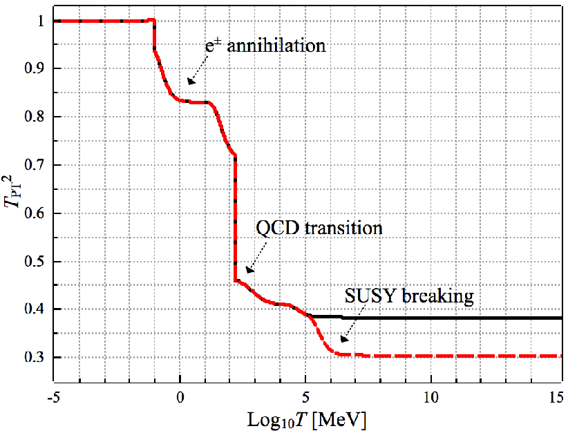
The cosmic phase transitions change the energy density of radiation thus the Hubble parameter , and affect the amplitude of RGWs through Eq. (9). The transfer function of phase transitions is [32, 31]
| (11) |
where is effective degree of freedom (here effective degree of freedom is obtained by converting all particles into effective photons, see Chapter 3.3 in [2]) for total energy density and is the effective degree of freedom for entropy density at temperature , while and are the present values. The parameter is the temperature at which the mode re-enters the horizon.
By use of the condition of horizon crossing and the conversation of entropy constant, we can convert temperature into wavenumber:
| (12) |
where K is the current CMB temperature [49] and is the redshift at . We can further convert wavenumber into frequency: .
The transfer function of phase transitions depends on not only the temperature but also the physical characteristics of particles, such as mass, degree of freedom and the statistical features (bosons or fermions) and so on. We follow the list of particles in [31] but update the data according to [50]. The temperature when particles decouple from the others is also very important. Here we adopt instantaneous decoupling of neutrinos from the radiation at MeV, and that electrons annihilate with positrons immediately at MeV [51]. The phase transition of QCD is treated as first order transition at 155 MeV [52].
Fig. 2 shows the square of transfer function at different temperature. When the cosmic phase transitions are considered, the energy density spectrum of RGWs can be reduced by about at MeV and by about at MeV. When we include the SUSY particles, the spectrum could be damped as much as at MeV. However, SUSY breaking is beyond the detecting ability of PTAs ( MeV). So we will not consider SUSY particles later.
II.3 Effects of relativistic free-streaming gases: neutrinos and dark fluids
II.3.1 Neutrinos
Now, let us discuss the anisotropic term in (2). As the cosmic magnetic filed is very small, we will ignore the magnetic sources [35]. When neutrinos decouple from the rest of radiation, the free streaming of neutrinos contributes to the anisotropic stress , which plays the role of friction in the equation of motion and damps the amplitude of RGWs, so it is necessary to study the damping effect of neutrinos.
In very high precision, the transfer function of relativistic free-streaming particles is [34, 36]
| (13) |
where is the fraction of free-streaming particles’ energy density over the total energy density. This formula applies for modes satisfying . When decreases and becomes comparable with , this formula does not apply any more. However, as decreases, the transfer function will gradually increases to 1 [53].
Because the sensitive band of PTAs is Hz, which is much higher than , we would not consider the behavior of free-streaming neutrinos near , thus (13) is enough for us and we take it as the transfer function of free-streaming particles.
When there are neutrinos only, is the fraction of energy density of free-streaming neutrinos. Before their decoupling from the radiation, , thus , so neutrinos could not damp the RGWs. After the decoupling, started to evolve with the Universe and depends on the temperature.
In Fig. 3, we plot the fraction of neutrinos’ energy density. We find that can be roughly divided into two constant stages with (before e annihilation) and with (after e annihilation). Therefore, our analysis is consistent with that in [29, 34]
It should be noted that the dip at and the spike at are artificial signatures. They are due to the imperfect deal with annihilation (we assume instantaneous annihilation here, which is not the real situation). The same artifacts appears in [31], while [54] explains this in its Appendix C.
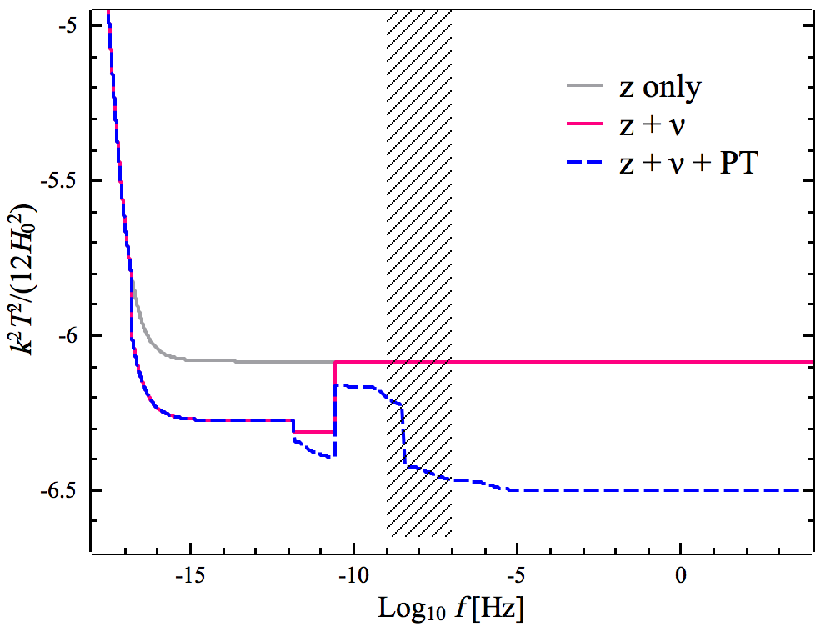
Fig. 4 plots the transfer function of cosmological redshift, neutrinos and cosmic phase transitions. Apparently, dominates all the damping effects in a wide range from Hz to Hz, while neutrino streaming would decorate the spectrum in the low frequency band (Hz) and the cosmic phase transitions modifies RGWs in the high frequency range (Hz). As we could see, phase transitions show their importance especially around Hz, which well resides in the sensitive band of PTAs.
II.3.2 Dark fluids
In the Standard Model of particle physics, there are three species of neutrinos. But when we consider the non-instantaneous decoupling of neutrinos, the effective number of neutrino species [55]. The current constraint from CMB and matter power spectra is (95% confidence) [56], while the BBN observations give (95% confidence) [57], so tension is still possible between theory and observation. Weinberg [58] proposed massless bosons to relax the tension and found for bosons decouple at MeV. Thus the current CMB observation can not exclude the existence of extra neutrino-like particles.

Here, we assume the existence of extra fermions to address the problem. Since massive particles freeze out at low temperature and do not contribute to , we would like to assume the particles are massless. Due to the constraints on , it is well justified to set the physical degree of freedom of dark fluid to be two (one for particle, the other for anti-particle), then . To consider the possibilities of different particles, we shall consider different decoupling temperature. Since the PTA band Hz corresponds to MeV, we consider three decoupling temperature and MeV in our discussion. As the extra particles can be any possible particles beyond current observations, we simply call them dark fluids (DFs).
Fig. 3 shows the fraction of free-streaming particles including dark fluid. When we include DF, becomes the fraction of all free-streaming particles’ energy density. Both neutrinos and dark fluid contribute to . Rich features occur in the fraction of free-streaming particles. In Fig. 3, we consider three different decoupling temperature ( and MeV) of dark fluid. Besides the two stages with and with separated by annihilation of at MeV, one more stage () appears when dark fluid decouples at or MeV, and a third stage ( with ) occurs when dark fluid decouples at MeV. Thus dark fluid would damp the RGWs at higher frequency.

By use of the expression of spectrum (8), the transfer function (10), (11) and (13), we can plot the energy density spectrum of RGWs for given and .
Fig. 5 shows the spectrum of energy density for , . In this plot we could see the damping effects caused by cosmological redshift, the cosmic phase transitions and the free-streaming neutrinos/DF. Neutrinos damp the spectrum at Hz, beyond the sensitive band of PTAs, thus PTAs cannot detect any relic signals from neutrinos. The cosmic phase transitions mainly damp the spectrum at Hz by amount of . The big jump at Hz is the signature of QCD phase transition ( MeV).
In Fig. 5, we find that DFs have three kinds of signature in the spectrum. Firstly, steps occur after their decoupling from the radiation. Secondly, the spectrum at Hz is damped more. Lastly, spectrum at Hz is raised.
At the moment of decoupling ( MeV), big jumps occur, as the free-streaming dark fluids start to damp the spectrum. In the range of the decoupling of neutrinos ( Hz), the appearance of dark fluid increases the fraction of free-streaming particles thus damps the spectrum more. This result is consistent with our intuition. But at higher frequencies (Hz) dark fluids raise the spectrum when compared to the case without dark fluids.
The reason why dark fluids raise the spectrum at high frequencies resides in the massless feature of dark fluid. We can clearly see this from the transfer function of phase transition (11). Massless particles can keep relativistic at low temperature and always contribute to the effective degree of freedom for energy and entropy density. So the addition of dark fluids increases the value of and . As for all (see Chapter 3.3 in [2]), then
| (14) |
At high temperature (which corresponds to high frequency) , so the increase of dominates and makes increase a bit.
II.4 Effects of general equation of state
After inflation, the Universe should experience a period of reheating to create the matter and dark matter we see today. Some time later, dark matter should decouple from the rest of particles [3]. It is suspected that this epoch before BBN can be dominated by massive particles and cause deviation from ideal fluid [34, 59], thus unusual EoS may occur. EoS could deeply change the shape of spectrum of energy density through scale factor as we would see below.
The relation between scale factor and conformal time could be generally parameterized by
| (15) |
where is related to the EoS parameter through
| (16) |
For the era of radiation domination, followed by , and for the era of matter domination, and . Since the EoS before BBN ( 1MeV) is still not clear, in the general scenario, we set as a free parameter, which represents the effective average EoS in this era.
The transfer function caused by general EoS is [26]
| (17) |
where is the scale factor at BBN epoch (here we chose the epoch at MeV without losing generality [2]) and is the Hubble parameter at BBN epoch. The lower boundary is determined by the fact that only those modes entered before are affected by unusual EoS.
Note that the sensitive band of PTA, i.e. Hz, corresponds to MeV, which is above the lower boundary of BBN energy scale, therefore unusual EoS could affect the detection of PTAs. In this sensitive frequency range, the tensorial index and the EoS are degenerate. To see this clearly, we put the transfer function of cosmic expansion and that of unusual EoS into the total transfer function. In the PTA sensitive band, , then from the spectrum (8) we find . The observations are influenced by the strength of RGWs, so they can merely determine the total tilt of , which is a combination of and .
Fig. 6 shows the spectrum of energy density undergoes the cosmic expansion and different EoS. For the unusual EoS with , the energy density spectrum of RGWs is strongly intensified, while the matter-like EoS () damps the RGWs greatly. It is clear that, when general EoS is considered, the spectrum at higher frequency is amplified or damped more than that at lower frequency.
Tab. 1 lists the exact strength of at three different frequencies. For the extremely stiff EoS with () , the strength could be amplified at least () times for the sensitive band of PTAs. For the mild EoS [59, 12], could be amplified times at Hz, and as far as times at Hz. While a matter-like EoS () may damp the strength by four orders of magnitude.
| Hz) | Hz) | Hz) | |

III Constraints on RGWs by current pulsar timing arrays
From Fig. 5 and Fig. 6, we have seen that many damping effects such as cosmological redshift, phase transition of QCD, the free-streaming dark fluids and the unusual EoS are well in the sensitive band of PTAs. Thus PTAs provide the good probe into these interesting physics. Now let us turn to the detection of RGWs through PTAs.
RGWs could weakly stretch or suppress the space, leading to the change of time of arrival for electro-magnetic pulses from pulsars. Difference of time of arrival could be accumulated to form considerable timing residuals. By analyzing the timing residuals carefully it is possible to detect RGWs.
In practice, the characteristic strain is more convenient for analysis and can be related to by [60]
| (18) |
So if the spectrum of energy density (8) is given, the characteristic strain can be determined theoretically.
When the spectrum is unknown, it is helpful to postulate a parameterized power-law form as follows [24, 23],
| (19) |
where is the amplitude of at Hz, and is the power index.

Fig. 7 shows the current constraints on from PPTA [22], EPTA [23] and NANOGrav [24]. From Fig. 7, we see that the result of PPTA is the most stringent one (about a factor of 1.5 better than NANOGrav at ), but there is only one data point (the black diamond in the figure), so in the rest part of this paper we would concentrate on results from NANOGrav and EPTA to cover more possible indices. In a wide range of , NANOGrav gives a tighter constraint than EPTA for all and the advantage becomes obvious as increases. For example, at , NANOGrav gives , which is only a factor of 1.7 better than of EPTA. When increases to , NANOGrav gives , a factor of 2.2 better than of EPTA.
III.1 Constraints on RGWs by current PTAs considering cosmic expansion only
When upper limits on for different indices are given, we can convert into through (18) and compare it with the theoretical results in (8) to give limits on the inflationary parameters and .
We should firstly find out the relation between the two power indices and . Because different damping effects alter the spectrum differently (see Fig. 5), the relation depends on the damping effects. Here we consider the spectrum damped by cosmic expansion only. In this case, the transfer function (7) has only one term from cosmic expansion (10). For waves with frequencies , we find the simple relation between and
| (20) |
and the relation between and
| (21) |
Inserting the parameters in Section II and the data in Fig. 7, we obtain the upper limits on for different .

Fig. 8 shows the constraints on space. The red dashed and the blue dashed line are the cases considering only. At , the limit from NANOGrav is , which is a factor of more stringent than from EPTA. Note that [23] gives a limit for the same EPTA data. The small deviation occurs because we adopt new cosmological parameters, which are slightly different from those used in [23]. As increases, the constraints become more stringent. At , the constraint of from NANOGrav is , while upper limit of EPTA is (see Table 2). For both constraints become very loose. In Table 2, we also list the results for .
For , when only redshift is considered, Zhao et al [25] found for NANOGrav [61] and for EPTA [62], based on the previous observations. While we found that, for , latest NANOGrav data [24] follows and EPTA data [23] follows . Both constraints become tighter due to the update of NANOGrav and EPTA data.
III.2 Constraints on RGWs by current PTAs considering phase transitions and neutrinos
Although the damping effects beyond cosmic expansion , such as cosmic phase transitions and the relativistic free-streaming gases , have been well studied before, few authors include these damping effects when they constrain the inflationary parameters (see [25] for example). As we mentioned before, cosmic phase transitions could damp the spectrum as much as 60% in the sensitive band of PTAs (see Fig. 5). Thus, to make accurate detection, it is inevitable to consider these damping effects. In this subsection, we will discuss the constraints on the inflationary parameters and when additional damping effects and are included in the transfer function.
There are two points that deserve our attention. Firstly, it is very clear that neutrinos could not affect any detection approached by PTAs, as neutrinos only damp the spectrum in the range of Hz, which is well beyond the detecting ability of PTAs. Secondly, makes the spectrum deviate from power law, so, strictly speaking, the postulation (19) does not hold. But is on the order of 0.1, which could only change the spectrum by a small amount, so in the meaning of perturbation, we could still apply the power law and attribute the small deviation from power law to the weak dependence of on the frequency. Then the relation (20) between and remains, while the expression of should be modified.
When we include cosmic phase transitions, the transfer function will have another term (11) besides (10), so the expression of becomes
| (22) |
As , we can expect the upper limit on for fixed would increase after we include cosmic phase transitions. Specifically, numerical calculations give , then we could obtain a looser constraint on space and the upper limit on increases a factor of 2.3 for all indices.
Fig. 8 shows the upper limit on . The red solid and the blue solid line are upper limits where is included. At , NANOGrav [24] gives upper limit , and EPTA [23] gives . Both are indeed raised by a factor of 2.3 compared to the limit without . At , the constraint from NANOGrav is and that given by EPTA is . We also list the results at in Table 2.
III.3 Constraints on RGWs from other observations
III.3.1 Constraints from BBN
Besides PTA projects, BBN can also give upper limit on space. BBN precisely predicts the abundance of light elements in the Universe. Nucleosynthesis happens efficiently when the collision rate of protons and neutrons are much higher than the Hubble parameter at that moment. To obtain enough abundance of H and He, the expansion rate of the Universe should not be too large, otherwise the plasma soup would be diluted too much to produce effective reaction. Expansion rate of the Universe or Hubble parameter depends on the energy density of radiation at that moment, thus the abundance of light elements could provide constraints on the total energy of radiation including RGWs.
By use of the effective number of neutrino species , BBN could set an upper limit on the energy of RGWs [60]
| (23) |
where is the number of neutrino species, while is the effective number of neutrino species. For standard model in particle physics, considering the non-instantaneous decoupling of neutrinos, [55]. Recent combined observations from BBN and primordial mass fraction of 4He and the abundance of deuterium give with confidence [57], then . The lower boundary of the integration is determined by counting the RGWs that entered horizon at the BBN epoch only, while the upper boundary is determined by quantum limit. For the very short wavelength (i.e. high frequency) portion, the ultraviolet divergences is avoided by considering the Parker’s adiabatic theorem [63], which states that, during a transition between expansion epochs with a characteristic time during , the gravitons created will be suppressed for wavenumbers . Here we follow [64] to choose Hz by assuming the energy scale for the inflation is around GeV and which can be obtained from (12).

Inserting the transfer function (10) caused by cosmic expansion and by cosmic phase transitions (11) into the spectrum of energy density in (8), we can integrate the spectrum numerically to obtain the upper limit on the inflationary parameter space . The result is shown by the purple dashed line in Fig. 9.
III.3.2 Constraints from CMB and matter power spectrum
Due to the precise observations of temperature and polarization anisotropies, in the modern cosmology, CMB becomes one of the most important tools to constrain various cosmological phenomena/processes including RGWs. RGWs affect the CMB fluctuations by two different ways.
Firstly, RGWs, as well as density perturbations, are the sources which generate the CMB anisotropy power spectra, including the temperature anisotropy auto-correlation spectrum (TT), E-mode polarization auto-correlation spectrum (EE), B-mode polarization auto-correlation spectrum (BB), and the cross-correlation of temperature anisotropy and E-mode polarization (TE). Although the definite signal of RGWs has not yet been found in the CMB power spectra, based on the recent observations of TT, TE and EE data, Planck team gives the quite tight constraint on the tensor-to-scalar ratio [7], which is nearly independent of the spectral index [65]. A similar constraint is also obtained from the joint analysis of BICEP2/Keck Array and Planck B-mode polarization data [10].
Secondly, RGWs affect the growth of density perturbation and the CMB anisotropy power spectra by contributing extra energy density to the total energy density or, equivalently, by changing the expansion rate of the Universe. The weak interaction of RGWs with matter makes them similar to massless neutrinos. So constraints on additional neutrinos from CMB and large-scale structure (LSS) observations could be applied to RGWs [66]. With confidence level, CMB combined with matter power spectra gives [56]. Again, we can insert this number into (23) to yield another constraints on RGWs. We obtain , but the lower boundary of integration is much lower than that of BBN. We adopt Hz [66] to do the integration. The corresponding constraint on is shown in Fig. 9 (the orange solid line).
III.3.3 Constraints from gravitational-wave detectors
The ground-based interferometer could directly detect RGWs in the range Hz by analyzing the interference stripes caused by gravitational waves in the laser beams. The latest constraints on the stochastic background is from joint observations of LIGO and Virgo. In frequency range Hz, LIGO and Virgo correlations give an upper limit on energy density spectrum for , while in the range Hz for (there are the other two sets of constraints at and , but they are much looser, so we ignore them). Both limits are of 95% confidence [12].
We can use the LIGO & Virgo data to estimate the upper limits of inflationary parameters and . Firstly, we convert the limits on at and into strain amplitude through (18), then use (22) to obtain limits on and at these two indices. Finally, we linearly fit the two points to cover the range in , which is shown in Fig. 9 (the black solid line).
III.3.4 Comparison with different constraints
Fig. 9 shows the constraints on space from different observations. We can see that at low index (), upper limit of from Planck is the most stringent and constant constraint (), while at high index (), constraint by use of joint analysis of CMB and LSS becomes the most stringent and the upper limit decreases as increases, for example, at , the upper limit is , but at , the limit is .
We see that the constraints from BBN (the purple dotted line) is slightly looser than that from the joint data of CMB and LSS (the orange solid line). There are two reasons for it. Firstly, constraints on from BBN is a bit looser than that from the joint analysis (0.36 versus 0.33, see subsection III.3.1 and III.3.2.) Secondly, the integration range of BBN ( Hz) is larger than that of the combination of CMB and LSS ( Hz), thus less energy could be added to the integration, making the tensor index larger.
Although the direct constraints from EPTA and NANOGrav have significantly improved recently, they are still much weaker than those from CMB, matter power spectra and BBN. So are LIGO and Virgo. Therefore, the great advancement is still needed to put tighter constraints. Advanced LIGO and future PTAs like FAST and SKA are indeed quite necessary.
IV Detection of RGWs by the future observations
In this section we will forecast the detections of RGWs by the potential PTA observations, including the FAST and SKA projects. In addition, as we know, the damping effects caused by cosmological redshift, phase transition of QCD, the free-streaming dark fluid and the unusual EoS are all well in the sensitive band of PTAs. So, the future PTAs also provide a good chance to study these interesting physics, which will also be investigated in this section.
In order to estimate detection abilities of the future PTAs, we will use time of arrival to establish the signal-to-noise ratio (SNR) of observations. When the spectrum of energy density (8) is given, an important problem follows: What confidence level can we achieve when we come up with new PTA projects to detect RGWs? The key lies on the timing residuals caused by RGWs and their correlations. RGWs could stretch or suppress the space weakly, leading to the change of time of arrival for electro-magnetic pulses from pulsars. Difference of time of arrival could be accumulated to form considerable timing residuals. The timing residuals are usually decomposed into two parts
| (24) |
where is the timing residual for -th pulsar at time , while and are the timing residuals contributed by RGWs and by noise. To make a detection, it is necessary to discriminate the contribution of RGW signal from that of noise. Let us consider the characteristic of and separately.
The genuine RGWs would induce common residuals in the data, so the correlation of gives [67]
| (25) |
where is Kronecker delta function and is the Hellings-Downs curve, while is root mean square (RMS) of timing residuals resulted from RGWs. The Hellings-Downs curve [20, 68] is
| (26) |
where is the angular separation between -th and -th pulsar. The RMS of timing residuals from RGWs is given by
| (27) |
where and are the lower and the higher boundary of sensitive band. and are the span of whole observation and the interval between two observations respectively. Now, if the spectrum of energy density (8) is given, the RMS of RGW is determined.
As for the part of noise, we assume that they are white and the same for every pulsar in the PTA, then the correlation of contributions from the noise is simple [67]
| (28) |
where is the RMS of timing residuals from white noise.
By use of the correlation of timing residuals and the whitening method, we could obtain the SNR for PTA [69, 25, 70]
| (29) |
where brackets are ensemble average (hereafter when we say SNR we mean the expectation of SNR, or ). is the number of pairs with being the number of pulsars. and are the average of and the variance of respectively. For pulsars evenly distributed in the full sky, we have .
As for , it is defined as the RMS in the -th bin [69]:
| (30) |
where is the bin whose signal is higher than noise, i.e. , with being the total number of observations in the PTA project. For the lower boundary of integration in is [69]. The total spectral density in a bin is the sum of contributions from signals and noises: .
We could see that, to calculate the SNR for a given spectrum of energy density, an observational plan should at least include the following information: the observation span , the number of pulsars , the number of observations and the noise level.
For timing noise, due to the intrinsic instability in the pulsars and uncertainties in the telescopes, the noise is not guaranteed to be white and may have different value for different pulsars [67]. In our analysis, for simplicity, we assumed white and equal noise level for all pulsars in a given array.
IV.1 Potential PTA projects in the future
In this paper, we follow Zhao et al [25] to consider the following future observations: the complete PPTA, FAST, SKA and optimal PTA.
The complete PPTA plans to observe 20 pulsars which have the same noise level of 100 ns over 5 years ( yr, ns, , ), while current PPTA mainly depends on four pulsars [22]. So the future PPTA could greatly improve the observation.
Another observation plan that deserves our attention is that from FAST, which would be the largest single dish in the world when it obtains the first light in 2016. Working with multi beams in the 70 MHz3GHz frequency band, FAST is expected to discover 4000 Galactic pulsars and one tenth may be millisecond pulsars [71]. For the search for gravitational waves, FAST plans to run a series of similar observations ( yr, , , we use FAST(20) to label this plan) but with much lower noise of only ns [71], which may directly improve the value of SNR. Here we assume a second plan, FAST(40), to adequately cover the possibility of more pulsars in a longer duration of timing: yr, , .
In the 2020s, the establishment of the thousands of single dishes will erect the biggest radio array SKA and pulsar searching and timing will be part of the SKA scientific goals. Accounting for the large signal-collecting area, SKA could well survey the pulsars in the Milky Way in an unprecedented efficient way [72] and greatly facilitate the detection of gravitational waves. To estimate the capacity of SKA in detecting RGWs, we adopt a low-noise plan running for ten years ( yr, ns, , we use SKA(100) to denote this plan) [73]. However, from a conservative view point, we would also consider a less ambitious one, SKA(40), with yr, ns, .
Prolonging time span allows PTAs to approach more low frequency signals, which can be much stronger than that of high frequency. So, accounting of these improvements, future PTAs may greatly increase their sensitivities. Zhao et al [25] also considered the optimal PTA ( yr, ns, ), which can reach an unprecedented sensitivity. For easy reference, we list these projects in Table 3.
| Potential PTA | /yr | /ns | ||
| Complete PPTA… | 5 | 100 | 20 | 250 |
| FAST(20)…………. | 5 | 30 | 20 | 250 |
| FAST(40)…………. | 10 | 30 | 40 | 500 |
| SKA(40)…………… | 10 | 50 | 40 | 500 |
| SKA(100)…………. | 10 | 50 | 100 | 500 |
| Optimal PTA……. | 20 | 30 | 200 | 1000 |
For the known damping factor, if and are given, the spectrum (8) is determined. Then, we use (18) to find the characteristic strain and obtain through (30) for known PTA observations. Finally, we can calculate the SNR for these observations through (29).

Note that without RGW signals, the timing residuals (24) will be Gaussian distributed, thus represents 95% confidence level. In the calculation, we would like to obtain the constraints on space with 95% confidence for the potential observations. This is possible, because for a given observational plans, when is fixed, and are constrained by the relation (29). So we firstly insert the spectrum with free parameters and into (18) to obtain through (30), then set to give upper limits on for different with 95% confidence level.
IV.2 Detecting RGWs in the accelerating Universe
As the first step, we only consider transfer function due to cosmic expansion in (10) and assume a normal radiation EoS before BBN in this section.
Fig. 10 show the SNR of FAST in the range . The black and grey lines are the SNR including damping effect from only. Our results for FAST(20) are the same as those in [25]. At , SNR vanishes for both FAST plans, thus no RGWs can be detected. However, as increases, the SNR increases a lot. If we fix , when , RGWs produce a significant detection with SNR for FAST(20) and 11.5 for FAST(40).
It is obvious that smaller leads to lower SNR. For example, at , when decreases from 0.1 to 0.001, SNR jumps from 11.5 to 6.5 for FAST(40), and from 4 to 2 for FAST(20), thus greatly weaken the detection.
The trends described above also hold for SKA, as we could see from Fig. 11, which shows the SNR for two SKA plans with 40 and 100 pulsars. Since the only difference between SKA(40) and SKA(100) is the number of pulsars (see Table. 3), we conclude that increasing the scale of arrays could greatly raise the detection ability. Lower noise level also increases the possibility to make a detection, therefore, FAST(40) will performe better than SKA(40). For example, at , for , FAST(40) gives SNR=11.5, which is a bit higher than 10 given by SKA(40).

In Fig. 12, we plot the constraints on space by potential observations. The dashed lines are the cases only considering . The current limits from NANOGrav and EPTA are also plotted here to make comparison. We could see, when only is considered, in the whole range , for the upper limits on , complete PPTA could be about times more stringent than current NANOGrav and about times better than current EPTA, while FAST(20) is times more stringent than complete PPTA and SKA(100) is 137 times better than FAST(20). The most stringent limit would come from the optimal PTA, which is about times better than SKA(100).
Although both SKA plans could defeat the FAST(20), the advantages of SKA would be greatly challenged by FAST(40), which is a factor of 2.5 better than SKA(40) and only a factor of 1.6 weaker than SKA(100). The good competence of FAST(40) comes from the low timing noise, as indicated by Table. 3. As SKA(100) and FAST(20) are the upper and lower limits of the four plans of SKA and FAST, we would concentrate on these two observations in the rest part of this paper. However, due to the similar resolution of FAST(40) and SKA(100) in the space, the results for SKA(100) also hold for FAST(40) with good accuracy.
At , upper limit on given by optimal PTA is , which is the best constraints. At , upper limit given by complete PPTA is , while FAST(20) gives and SKA(100) and the optimal PTA are much more stringent.

For , the optimal PTA gives , while for SKA(100) the upper limit is , for FAST(20) it is , and for complete PPTA, it is . If , the optimal gives limit , SKA(100) gives , and FAST(20) gives . So both SKA(100) and optimal PTA could give fairy good constraints on the inflation models.
IV.3 Effects of phase transitions and neutrinos
In the previous work [25], we only calculated the SNR for the RGWs damped by cosmic expansion , which is briefly reviewed in the previous subsection. However as we mentioned before, cosmic phase transitions, especially the phase transition of QCD, damp the spectrum by amount of 60% at Hz, which is well in the sensitive band of PTAs. Relativistic free-streaming neutrinos could also damp the spectrum by about 40% in the range of Hz. Although the behavior of neutrinos has no effect on PTAs, they play an important role in the constraints by use of combined CMB and matter power spectra. Therefore effects from cosmic phase transitions and neutrinos deserve attention.
In this subsection, we shall take into account the damping effects caused by cosmic phase transitions in (11) and neutrinos in (13). Here we also assume a normal EoS with .

For PTAs we only deal with the effects of due to QCD transition and ignore the damping effects of annihilation and SUSY breaking, as annihilation affects RGWs in the range of Hz (or, equivalently, MeV) and SUSY phase transition in the range of Hz (or MeV). We add the transfer function and to the total transfer function, and follow the procedures described in Section IV.1 to obtain SNR and the constraints on and respectively.
In Fig. 10, the red and orange lines show the SNR for RGWs further damped by in FAST plans. Obviously, compared with the cases which only contain , SNR decreases for both plans when additional cosmic phase transitions are considered. The decline of SNR is consistent with our intuition, as additional damping could surely lead to weaker RGW signals and smaller SNR. In each observation, when , for , SNR decreases by an almost constant amount: FAST(40) decreases one unit, while FAST(20) by amount of 0.6. So cosmic phase transitions are more important in FAST(40) than in FAST(20). As decreases, the difference in SNR caused by also decreases and tends to zero at . Similar features appear in SKA observations too (see Fig. 11).
Fig. 12 shows the effects of cosmic phase transitions on parameters and . Obviously, raises the upper limits of all PTAs nearly by a constant factor of in the wide range of . It is not difficult to understand the reason, as the big jump cased by QCD transition is the main feature in the narrow sensitive band of PTA (see Fig. 5).
In Fig. 13, we put the constraints from future PTAs and those from current observations together to get a better view. The bounds from PTAs have already included damping effects from cosmic expansion and phase transitions . We see that around , SKA(100) could do much better in limiting and become very competitive with current CMB observations from Planck and the joint analysis from CMB and LSS. In , SKA(100) is a bit more (about a factor of ) stringent than BBN and CMB. In comparison with constraints from CMB and BBN, the role of cosmic phase transitions becomes particularly important for SKA(100), because if without the advantage of SKA(100) could increase to about times better than CMB and BBN over a wider range. We can also find that optimal PTA could replace the dominant role of CMB and BBN in the range and restrict for and for , which are very tight limits for a wide variety of inflation models, including slow-rolling inflation. We list the upper limits on in Table 4 for clarity. When we fix , we see that at , CMB is still most stringent constraints even for the optimal PTA, but for a small positive tensorial index. e.g. , the optimal PTA can require . Therefore, the future constraints are much better than the present ones if the spectrum of RGWs is blue tilted (i.e. ). The bounds on for different indices are listed in Table 5.
| upper limit on | ||
| without | with | |
IV.4 Effects of relativistic free-streaming dark fluids
The possible excess of effective number of neutrino species leads to tension between observations and theories. As we mentioned in Sec. II.3.2, this problem may be reconciled by assuming extra relativistic light particles, such as massless bosons proposed by [58] or a class of massless fermions i.e. the dark fluid in this paper. If verified, the existence of extra species of particles will bring new physics both to particle physics and cosmology.
For RGWs, we have found that dark fluid plays dual roles in the evolution of the gravitational waves (see Fig. 5): It damps the spectrum by adding the fraction of free-streaming particles (see Fig. 3). Meanwhile, it raises the RGW spectrum a bit through cosmic phase transitions (see Eq. (14)).

In this subsection, we will focus on the impact of dark fluid on SNR and constraints on space. As before, we also assume an EoS with before BBN. Since dark fluid could affect the spectrum through both cosmic phase transition and free-streaming gases, we should combine the transfer function , and to get the total transfer function in the spectrum (8), then perform the similar procedures depicted in Sec. IV.1 to calculate SNR of RGWs for different potential observations.
Fig. 14 shows the difference on SNR of SKA(100) caused by dark fluids decoupling at and MeV. It is not strange to find that dark fluid can raise the SNR curve a bit (), as dark fluid could raise the spectrum through phase transition and counteract the damping effect caused by its free-streaming (see Eq. (14)). We could see this clearly in Fig. 5: For the dark fluid decoupling at MeV (the black solid line, which is partially covered by the green solid line for MeV), the spectrum in the PTA band is clearly raised a bit, while for that decouples at MeV (the blue dashed line), the spectrum is not only raised a bit at the high frequency end (i.e. Hz), but also damped a bit at the frequencies below QCD transition (i.e. Hz). While at the middle frequencies ( Hz), the two effects nearly cancel each other. For dark fluids that decouple at MeV, the effect of free-streaming could extend to higher frequencies, making the spectrum nearly unchanged. Therefore the SNR for the case of and MeV are raised more than that for MeV (the spectrum for MeV increases because the effect near Hz become dominant as ). This is consistent with Fig. 14, where the SNR curve for dark fluid decoupling at MeV (the purple solid line) is the middle one between the curve for MeV (the green dotted line) and that without dark fluid (the orange solid line).
As goes up to , the spectrum could be raised more by dark fluids, because the contribution of high frequencies become dominant for . We find the largest influence on SNR caused by dark fluid for , but the SNR of SKA(100) is only raised by less than for . Obviously, the impact on FAST would be even smaller (similar to the cases in Fig. 10). So the influence of dark fluid could reasonably be ignored by PTAs and we cannot expect any significant changes caused by dark fluid in the space.
The reason why dark fluid plays small influence on the spectrum is simple. Current constraints on the number of species is so stringent that only one or two more kinds of extra particles are allowed, thus the contribution of dark fluid to the total radiation around the PTA band (Hz, or equivalently, MeV) is quite small, so both phase transition and free-streaming of dark fluid become insignificant.
IV.5 Effects of different equation of state
BBN could trace physics up to about 10 MeV in the history of Universe. However, the physics above this energy scale is not quite clear, for example, EoS in this range is not determined. Reheating after inflation and the appearance of massive particles may lead to quite interesting EoS, which could make the Universe evolve differently. For RGWs, these unusual EoS may greatly amplify or depress the amplitudes, making the detection hopeful or despaired (see Fig. 6). With the advancement in the detection of RGWs, more stringent constraints could be set to the EoS in this early stage of the Universe and limit the possible reheating physics.
Since the transfer function of unusual EoS alters the RGW spectrum dramatically (up to several orders of magnitude), we will neglect the damping effects induced by cosmic phase transitions and free-streaming particles in this subsection, and only consider effects caused by cosmic expansion and unusual EoS . Similar to the previous works [26, 12], we will consider five different EoS with and to cover the stiff, soft and radiation-like states.

Firstly, we consider, when unusual EoS appears, to what extent the current NANOGrav data can limit the space. With procedures similar to (21) and (22), we could find the expression of . Then by use of the NANOGrav data (see Fig. 7), we can calculate the upper limits on for the unusual EoS mentioned above. Fig. 15 shows the constraints on space when both and are considered. We can see that stiff EoS () could greatly suppress the possible parameter space. For example when , the upper limit on is for and for , both of which are more compact than that of for . The upper limit could even be pushed to for .
Now we consider the potential constraints from the future PTAs. Inserting the transfer function of unusual EoS and of cosmic expansion to the total transfer function in the RGW spectrum, we could follow the steps given in Sec. IV.1 to calculate the SNR and the constraint on for different observations.

Fig. 16 shows the SNR for different EoS in the SKA(100) project. We can see that, compared with the normal EoS of radiation (), stiff EoS () could greatly increase the SNR of PTAs in the whole range of . SNR even starts to saturate with SNR = 67.1 at for the infinity stiff EoS, and reaches maximum at for . Around , SNR for and infinity can reach a well level. For example, when , we have SNR=2 for . Therefore, SKA(100) is still very sensitive to the EoS above . If the EoS before BBN is dominated by matter of , then the SNR will be dramatically damped in the whole range of and the maximum of SNR is at . So, in conclusion, RGWs are quite sensitive to the EoS before BBN and could provide good probes into the interesting physics in this epoch.
Fig. 17 shows the constraints on for SKA(100) when different EoSs are considered. We could see that, stiff EoS with makes the constraints more stringent than the case of , while the matter-like EoS () damps the spectrum so much that the constraint becomes very loose. Explicitly, at , the upper limit on given by is less than , while gives , and gives , all of which are more stringent than given by normal radiation-like EoS (), but if , the upper limit on is near 1. So we can conclude that stiff EoS could facilitate the constraints of RGW parameters. For the case of , and , we list the constraints on in Table 6.
| upper limit of | |||

V Conclusions
A stochastic background of relic gravitational waves, generated during the early inflationary stage, is a necessity dictated by general relativity and quantum mechanics. The spectrum of RGWs directly depends on the inflationary physics. So, it is always treated as the smoking-gun evidence of inflation. In addition, in the post-inflation stage, various cosmic phase transitions and relativistic free-steaming gases, also left imprints on the RGW spectrum. For this reason, RGWs also provide the cleanest way to probe the physics in the post-inflation epoch.
Detections of RGWs have been carried on by different experimental methods. In the median frequency range Hz, the detection is by analyzing the timing residual of the millisecond pulsars. Recently, all three PTA groups (PPTA, EPTA and NANOGrav) reported the latest constraints on the GW background. In this paper, by considering the current and the potential future PTA observations, we investigated the constraints on the RGWs and the inflationary parameters in the general cosmological scenario. In particular, we studied the effects of cosmic phase transitions and various relativistic free-streaming fluids, which had been neglected in all the previous works.
Cosmic phase transitions, including annihilation, QCD transition and SUSY breaking, damp the RGW spectrum in the frequency range Hz, which is exactly the sensitivity range of PTA method. Taking into account the damping effects caused by all physical transitions, we find the upper limit of the tensor-to-scalar ratio increases by a factor for any given spectral index . In the standard cosmological scenario, for current NANOGrav constraints with , the upper limit of increases from to . While, for the future SKA(100), if , we find the detection of RGWs is possible only if , instead of .
The relativistic free-streaming gases, including neutrinos and some unknown dark fluids in the Universe, influenced the evolution of RGWs in the radiation-dominant stage, which significantly damped the RGWs spectrum at the frequency range Hz. By analysis, we find this effect is very small in frequency Hz for both neutrinos and dark fluids. Even for the future SKA(100) project, this effect seems impossible to be detected.
In the general cosmological scenario, the effective EoS of the cosmic fluid can be different from in the pre-BBN stage. We find that, the value of greatly affects the RGWs spectrum, as well as their detection by pulsar timing arrays. For the future SKA(100) project, if is set, we find the detection is possible if for the standard model with . However, if , they can be detected only if . So, the stiff EoS could significantly decreases the difficulties of RGW detection.
At the end of this paper, we should mention that in addition to the detection methods above, RGWs have also been constrained by some other observational and experimental efforts. In the frequency range Hz, GW background produces a pattern of apparent proper motion of quasars. So, by observing the motion of quasars in the Universe, an interesting constraint in this frequency band is given in [74]. For the RGWs with high frequency Hz, by analyzing the implications of graviton to photon conversion in the presence of large-scale magnetic fields, an upper limit is derived in [75]. Meanwhile, the experimental detections of the RGWs by various GW detectors (e.g. the cryogenic resonant bar detectors [76], the cavity detectors MAGO[77], the waveguide detectors [78], the Gaussian maser beam detectors [79]) have also been well studied in the recent literatures.
Acknowledgements: This work is supported by Project 973 under Grant No. 2012CB821804 and 2014CB845806, by NSFC No. 11173021, 11322324, 11421303, 11275187, 11421303, 11373014 and 11073005, SRFDP, CAS, the Strategic Priority Research Program ¡±The Emergence of Cosmological Structures ¡± of the Chinese Academy of Sciences, Grant No. XDB09000000, and the Fundamental Research Funds for the Central Universities and Scientific Research Foundation of Beijing Normal University.
References
- [1] A. H. Guth, Phys. Rev D 23, 347 (1981).
- [2] E. W. Kolb and M. S. Turner, The Early Universe (Westview Press, Boulder, CO, 1990).
- [3] S. Weinberg, Cosmology (Oxford University Press, New York, 2008).
- [4] V. F. Mukhanov, H. A. Feldman, and R. H. Brandenberger, Phys. Rept. 215, 203 (1992); D. H. Lyth and A. Riotto, Phys. Rept. 314, 1 (1999).
- [5] D. N. Spergel, et al. (WMAP Collaboration), Astrophys. J. Suppl. 148, 175 (2003); E. Komatsu et al. (WMAP Collaboration), Astrophys. J. Suppl. 192, 18 (2011); G. F. Hinshaw et al. (WMAP Collaboration), Astrophys. J. Suppl. 208, 19 (2013).
- [6] P. A. R. Ade et al. (Planck Collaboration), A&A 571, A1 (2014); P. A. R. Ade et al. (Planck Collaboration), A&A 571, A16 (2014); N. Aghanim et al. (Planck Collaboration), arXiv:1507.02704.
- [7] P. A. R. Ade et al. (Planck Collaboration), arXiv:1502.01589; P. A. R. Ade et al. (Planck Collaboration), arXiv:1502.02114.
- [8] L. P. Grishchuk, Sov. Phys. JETP 40, 409 (1975); Ann. N. Y. Acad. Sci. 302, 439 (1977); JETP Lett. 23, 293 (1976); A. A. Starobinsky, JETP Lett. 30, 682 (1979); Phys. Lett. B 91, 99S (1980).
- [9] A. G. Polnarev, Soviet Astronomy, 29, 607 (1985); U. Seljak and M. Zaldarriaga, Phys. Rev. Lett. 78, 2054 (1997); M. Kamionkowski, A. Kosowsky, and A. Stebbins, Phys. Rev. Lett. 78, 2058 (1997); W. Zhao, D. Baskaran and L. P. Grishchuk, Phys. Rev. D 79, 023002 (2009); W. Zhao and L. P. Grishchuk, Phys. Rev. D 82, 123008 (2010).
- [10] P. A. R. Ade et al. (BICEP2/Keck and Planck Collaborations), Phys. Rev. Lett. 114, 101301 (2015).
- [11] J. Bock et al. Task Force on Cosmic Microwave Background Research, arXiv:astro-ph/0604101; W. Zhao, JCAP, 1103, 007 (2011).
- [12] J. Aasi et al. (LIGO and Virgo Collaboration), Phys. Rev. Lett. 113, 231101 (2014).
- [13] http://www.advancedligo.mit.edu
- [14] http:/www.et-gw.eu
- [15] P. Amaro-Seoane et al., arXiv:1201.3621.
- [16] http://universe.nasa.gov/program/bbo.ttml.
- [17] N. Seto, S. Kawamura and T. Nakamura, Phys. Rev. Lett. 87. 221103 (2001).
- [18] W. T. Ni, S. Shiomi and A. C. Liao, Classical Quantum Gravity 21, S641 (2004).
- [19] M. V. Sazhin, Soviet Astronomy, 22, 36 (1978); S. Detweiler, Astrophys. J. 234, 1100 (1979).
- [20] R. W. Hellings and G. S. Downs, Astrophys. J. 265, L39 (1983).
- [21] R. S. Foster and D. C. Backer, Astrophys. J. 361, 300 (1990).
- [22] R. M. Shannon et al., Science, 349, 1522 (2015).
- [23] L. Lentati et al. (EPTA Collaboration), Mon. Not. Astron. Soc. 453, 2576 (2015).
- [24] Z. Arzoumanian et al. (NANOGrav Collaboration), arXiv:1508.03024.
- [25] W. Zhao, Y. Zhang, X. P. You and Z. H. Zhu, Phys. Rev. D 87, 124012 (2013).
- [26] W. Zhao, Phys. Rev. D 83, 104021 (2011).
- [27] M. L. Tong, Y. Zhang, W. Zhao, J. Z. Liu, C. S. Zhao and T. G. Yang, Glassical Quantum Gravity 31, 035001 (2014).
- [28] M. L. Tong and Y. Zhang, Phys. Rev. D 80, 084022 (2009).
- [29] S. Weinberg, Phys. Rev. D 69, 023503 (2004).
- [30] W. Zhao, Y. Zhang and T. Y. Xia, Phys. Lett. B 677, 235 (2009).
- [31] Y. Watanabe and E. Komatsu, Phys. Rev. D 73, 123515 (2006).
- [32] W. Zhao, Chinese Physics, 16, 2894 (2007).
- [33] S. Wang, Y. Zhang, T. Y. Xia and H. X. Miao, Phys. Rev. D 77, 104016 (2008).
- [34] L. A. Boyle and P. J. Steinhardt, Phys. Rev. D 77, 063504 (2008).
- [35] R. Maartens, C. Tsagas and C. Ungarelli, Phys. Rev. D 63, 123507 (2001).
- [36] D. A. Dicus and W. W. Reoko, Phys. Rev. D 72, 088302 (2005).
- [37] H. V. Peiris et al. (WMAP Collaboration), Astrophys. J. Suppl. 148, 213 (2003).
- [38] S. Dodelson, Modern Cosmology (Academic Press, 2003).
- [39] D. Baumann and L. McAllister, arXiv: 1404.2601
- [40] Y. S. Piao, Phys. Rev. D73, 047302 (2006); T. Biswas and A. Mazumdar, Classical Quantum Gravity 31, 025019 (2014); E. J. Copeland, N. J. Nunes and M. Shaeri, Phys. Rev. D 77, 023510 (2008), Phys. Rev. D 79, 023508 (2009); F. Briscese, A. Marciano, L. Modesto and E. N. Saridakis, Phys. Rev. D 87, 083507 (2013); D. Cannone, G. Tasinato and D. Wands, JCAP 1501, 029 (2015); Y. Cai, J. Gong, S. Pi, E. N. Saridakis and S. Wu, arXiv: 1412.7241
- [41] Y. Zhang, X. Z. Er, T. Y. Xia, W. Zhao and H. X. Miao, Classical Quantum Gravity 23, 3783 (2006).
- [42] M. S. Turner, M. White and J. E. Lidsey, Phys. Rev. D 48, 4613 (1993).
- [43] W. Zhao and Y. Zhang, Phys. Rev. D. 74, 043503 (2006).
- [44] E. D. Stewart and D. H. Lyth, Phys. Lett. B 302, 171 (1993).
- [45] Y. Zhang, Y. Yuan, W. Zhao and Y. T. Chen, Classical Quantum Gravity 22, 1383 (2005).
- [46] S. Chongchitnan and G. Efstathiou, Phys. Rev. D 73, 083511 (2006).
- [47] M. Giovannini, PMC Phys.A 4 1 (2010)
- [48] S. Kuroyanagi, C. Gordon, J. Silk and N. Sugiyama, Phys. Rev. D 81, 083524 (2010).
- [49] D. J. Fixsen, Astrophys. J. 707, 916 (2009).
- [50] K. Olive et al. (Particle Data Group), Chin. Phys. C, 38, 090001 (2014).
- [51] V. Mukhanov, Physical Foundations of Cosmology, (Cambridge University Press, 2005).
- [52] T. Bhattacharya et al. (Hot QCD Collaboration), Phys. Rev. Lett. 113, 082001 (2014).
- [53] B. A. Stefanek and W. W. Repko, Phys. Rev. D 88, 083536 (2013).
- [54] S. Kuroyanagi, T. Chiba and N. Sugiyama, Phys. Rev. D 79, 103501 (2009).
- [55] G. Mangano, G. Miele, S. Pastor and M. Peloso, Phys. Lett. B 534, 8 (2002).
- [56] L. Pagano, L. Salvati and A. Melchiorri, arXiv: 1508.02393.
- [57] R. H. Cyburt, B. D. Fields, K. A. Olive and T. H. Yeh, arXiv:1505.01076.
- [58] S. Weinberg, Phys. Rev. Lett. 110, 241301 (2013).
- [59] L. A. Boyle and A. Buonanno, Phys. Rev. D 78, 043531 (2008).
- [60] B. Allen and J. D. Romano, Phys. Rev. D 59, 102001 (1999); M. Maggiore, Phys. Rept. 331, 283 (2000).
- [61] P. B. Demorest et al., Astrophys. J. 762, 94 (2013).
- [62] R. van Haasteren et al., Mon. Not. Astron. Soc. 414, 3117 (2011).
- [63] L. Parker, Phys. Rev. 183, 1057 (1969).
- [64] H. Miao and Y. Zhang, Phys. Rev. D 75, 104009 (2007).
- [65] Q. G. Huang and S. Wang, JCAP 06, 021 (2015).
- [66] T. L. Smith, E. Pierpaoli and M. Kamionkowski, Phys. Rev. Lett. 97, 021301 (2006).
- [67] K. J. Lee, C. G. Bassa, G. H. Janssen, R. Karuppusamy, M. Kramer, R. Smith and B. W. Stappers, Mon. Not. Roy. Astron. Soc. 423, 2642 (2012).
- [68] K. J. Lee, F. A. Jenet and R. H. Price, Astrophys. J. 685, 1304L (2008).
- [69] F. A. Jenet, G. B. Hobbs, K. J. Lee and R. N. Manchester, Astrophys. J. 625, L123 (2005).
- [70] S. Kuroyanagi, K. Miyamoto, T. Sekiguchi, K. Takahashi and J. Silk, Phys. Rev. D 87, 023522 (2013).
- [71] R. Nan, D. Li, C. Jin, Q. Wang, L. Zhu, W. Zhu, H. Zhang, Y. Yue and L. Qian, Int. J. Mod. Phys. D 20, 989 (2011).
- [72] M. Kramer, New horizons in time-domain astronomy. IAU Symp. 285, 147 (2012)
- [73] A. Sesana and A. Vecchio, Classical Quantum Gravity, 27, 084016 (2010).
- [74] T. Pyne, C. R. Gwinn, M. Birkinshaw, T. M. Eubanks and D. N. Matsakis, Astrophys. J. 465, 566 (1996); C. R. Gwinn, T. M. Eubanks, T. Pyne, M. Birkinshaw and D. N. Matsakis, Astrophys. J. 485, 87 (1997).
- [75] M. S. Pshirkov and D. Baskaran, Phys. Rev. D 80, 042002 (2009).
- [76] P. Astone et al., Classical Quantum Gravity, 25, 114028 (2008); P. Astone et al., Astropart. Phys. 7, 231 (1997), Classical Quantum Gravity 25, 184012 (2008).
- [77] R. Ballatini et al., arXiv:gr-qc/0502054, INFN Technical Note INFN/TC-05/05 (2005).
- [78] A. M. Cruise, Classical Quantum Gravity 17, 2525 (2000); A. M. Cruise and R. M. J. Ingley, Classical Quantum Gravity 22, S479 (2005), 23, 6185 (2006); M. L. Tong and Y. Zhang, Chin. J. Astron. Astrophys. 8, 314 (2008).
- [79] F. Y. Li, M. X. Tang and D. P. Shi, Phys. Rev. D 67, 104008 (2003); F. Y. Li et al., Eur. Phys. J. C 56, 407 (2008); M. L. Tong, Y. Zhang and F. Y. Li, Phys. Rev. D 78, 024041 (2008); F. Y. Li, H. Wen and Z. Y. Fang, arXiv:1505.06546.