Efficient, uninformative sampling of limb-darkening coefficients for a three-parameter law
Abstract
Stellar limb-darkening impacts a wide range of astronomical measurements. The accuracy to which it is modelled limits the accuracy in any covariant parameters of interest, such as the radius of a transiting planet. With the ever growing availability of precise observations and the importance of robust estimates of astrophysical parameters, an emerging trend has been to freely fit the limb-darkening coefficients (LDCs) describing a limb-darkening law of choice, in order to propagate our ignorance of the true intensity profile. In practice, this approach has been limited to two-parameter limb-darkening laws, such as the quadratic law, due to the relative ease of sampling the physically allowed range of LDCs. Here, we provide a highly efficient method for sampling LDCs describing a more accurate three-parameter non-linear law. We first derive analytic criteria which can quickly test if a set of LDCs are physical, although naive sampling with these criteria leads to an acceptance rate less than 1%. We then show that the loci of allowed LDCs can be transformed into a cone-like volume, from which we are able to draw uniform samples. We show that samples drawn uniformly from the conal region are physically valid in 97.3% of realizations and encompass 94.4% of the volume of allowed parameter space. We provide python and fortran code (ldc3) to sample from this region (and perform the reverse calculation) at this http, which also includes a subroutine to efficiently test whether a sample is physically valid or not.
Keywords:
methods: analytical — methods: statistical — stars: atmospheres.1 INTRODUCTION
Stellar limb-darkening affects a wide range of astronomical observations, such as exoplanetary transits (Mandel & Agol, 2002), microlensed light curves (e.g. Witt 1995; Zub et al. 2011), rotational modulations (Kipping, 2012), ellipsoidal variations (Morris & Naftilan, 1993), interferometric images of stars (e.g. Aufdenberg et al. 2005) and eclipsing binaries (Kopal, 1950). When interpreting such observations, the assumed shape of the limb-darkening intensity profile may significantly affect the inferred parameters of interest (Csizmadia et al., 2013). Consequently, an accurate treatment of limb-darkening is crucial, even when the effect itself is a “nuisance” phenomenon.
In many practical cases, limb-darkening is treated by describing the stellar intensity profile with a closed-form analytic model. This model is usually called the “limb-darkening law”, which is designed to provide an accurate analytic approximation the true profile. The major advantage of modelling the intensity profile analytically is that the astronomical phenomena under investigation may also be modelled analytically, offering computational expedience and greater physical insight. As an example, in the field of exoplanet transits, the shape of a transit light curve can be described with a closed-form, analytic model under the assumption of a polynomial-based description of the stellar intensity profile (Mandel & Agol, 2002; Giménez, 2006).
All of the commonly used limb-darkening laws may be described as a linear sum of one or more simple functions, each of which is weighted by a so-called limb-darkening coefficient (LDC). For example, the popular quadratic limb-darkening law describes the intensity profile as a quadratic series expansion with respect to the angle between the line of sight and the emergent intensity () and has two LDCs (Kopal, 1950). These LDCs control the shape of the intensity profile, subject to the flexibility granted by the limb-darkening law’s complexity. It is therefore necessary to make at least two major decisions with how to treat limb-darkening; what limb-darkening law should be used and what LDCs should be assigned to this law?
A typical approach for assigning LDCs is to adopt a set of so-called “theoretical” LDCs. In this framework, one first simulates an intensity profile using a sophisticated stellar atmosphere model at a particular wavelength or over a chosen integrated bandpass. One then takes this simulation and regresses the limb-darkening law of choice to it by finding the maximum likelihood set of LDCs (in some instances the LDCs are restricted to ensure physically sound profiles). Since the simulated profile is sensitive to several parameters defining the stellar surface (e.g. effective temperature, metallicity, surface gravity), several groups have produced grid tabulations of LDCs for a wide range of plausible inputs and assumed limb-darkening law (e.g. see Van Hamme 1993, Díaz-Cordovéz et al. 1995, Claret 2000 and Sing 2010).
In recent years, there has been a shift away from using theoretical LDCs in favour of freely fitting LDCs simultaneous to the exploration of the other parameters of interest (e.g. Knutson et al. 2007, Kipping & Bakos 2011a; Kipping & Bakos 2011b and Kreidberg et al. 2014). This approach, enabled by advances in modern computers, allows one to propagate our ignorance regarding the shape of the intensity profile into the estimation of the parameters of interest, leading to more accurate estimates parameter uncertainties. Such a procedure also allows one to decouple from any possible errors in the stellar atmosphere models themselves, which have been shown to sometimes be inconsistent with observed limb-darkening profiles (Howarth, 2011; Epinoza & Jordán, 2015).
One major challenge when attempting to freely fit LDCs is that many combinations of the LDCs are unphysical. For example, a specific choice of LDCs may result in the intensity profile being occasionally negative. These regions of unphysical parameter space may coincide with likelihood minima, leading to erroneous parameter posterior distributions. Softer, extended likelihood minima (typical of low signal-to-noise data) may spill over into the unphysical parameter space, causing the final parameter posteriors to be marginalized over large swaths of unphysical parameter space leading to unnecessarily swollen error bars.
There are two solutions to this problem. The first is to define a set of criteria which quickly allow us to identify forbidden combinations of the LDCs. Armed with such criteria, one could then test each realization and accept or reject the realization accordingly. This works fine unless the volume of forbidden parameter space is large, in which case one will severely impede a regression algorithm’s efficiency since most trials are being rejected as unphysical. A more elegant solution is to directly sample exclusively (or at least efficiently) from the physically allowed volume of parameter space (and also in such a way that the LDCs can be uniformly, or nearly uniformly, sampled). This provides the benefits of a very high efficiency, physically sound priors and no need for testing criteria at each realization. However, this approach comes at the cost of the initial intellectual investment to actually solve how to perform efficient sampling in the first place.
Because direct sampling of physical LDCs is challenging, the most complex limb-darkening law for which this feat has yet been achieved is the simple quadratic law, where the intensity profile of the star is given by
| (1) |
where is the specific intensity at the centre of the disc, and are the quadratic LDCs and is the cosine of the angle between the line of sight and the emergent intensity. In Kipping (2013), we showed that physically sound and LDCs reside within a triangle on the - plane, from which uniform samples can be easily drawn by re-parameterizing to and . Other simple two-parameter laws were considered as well in this work.
Despite these successes with two-parameter laws, these laws are fundamentally limited in their ability to accurately describe realistic limb-darkening profiles. This translates to systematic uncertainty in any and all model parameters which are covariant with the limb-darkening properties. This may, for example, limit our ability to accurately measure the radius of a transiting exoplanet and thus make inferences of its composition. We are therefore motivated to extend the Kipping (2013) analysis to a more sophisticated limb-darkening law.
The most accurate closed-form limb-darkening law is the Claret (2000) four-parameter non-linear law, described by
| (2) |
In numerous independent studies, this law has been found to provide the most accurate description of simulated intensity profiles (e.g. Claret 2000, Sing 2010 and Magic et al. 2015) versus competing models. This is, however, not surprising since this law also utilizes the greatest number of LDCs. Analytically identifying the unphysical combinations of these four LDCs remains an outstanding and formidable challenge. A more tractable problem that we consider in this work is the allowed volume of LDCs (and methods to directly sample from said volume) in the case of the Sing et al. (2009) three-parameter law:
| (3) |
Sing (2010) argues that dropping the term is motivated by solar data (Neckel & Labs, 1994) and 3D stellar models (Bigot et al., 2006), which show that varies smoothly at small , meaning that a term is superfluous. We therefore argue that the Sing et al. (2009) law offers both a significant improvement in accuracy and yet is simple enough for us to analytically constrain the allowed LDCs.
2 PHYSICAL CRITERIA
2.1 Physical Conditions
We define the following physical conditions with respect to a limb darkened stellar intensity profile:
- (I)
an everywhere-positive intensity profile,
- (II)
a monotonically decreasing intensity profile from the centre of the star to the limb,
- (III)
the intensity profile has a negative curl at the limb.
Physical conditions I and II are the same two imposed in our previous paper, Kipping (2013). As noted in that work, limb brightening is possible for narrow-band observations (e.g. see Schlawin et al. 2010) and such behaviour is not considered in this work either. Physical condition III is motivated by the expectation that the intensity rapidly drops off towards the limb (and is discussed in more detail later in §2.5). Throughout this work, we refer to a set of LDCs satisfying these three conditions as being physical, and LDCs otherwise are defined as unphysical. In what follows, we explore the consequences of these simple constraints.
2.2 Criterion A
Physical condition I demands that . We begin by evaluating this condition at two extrema of and , in a similar manner to the approach adopted in Kipping (2013):
| (4) |
The upper line clearly has no constraining power, but the second line provides our first criterion of
| (5) |
2.3 Criteria B and C
Next, we consider physical condition II, which demands that :
| (6) |
As was done in the previous subsection, let us evaluate the above in the extreme cases of and , yielding
| (7) |
These two expressions provide our criteria B and C, which are respectively given by
| (8) |
and
| (9) |
2.4 Criterion D
Physical condition II tells us that the intensity decreases from the centre of the star to the limb. This implies that the intensity everywhere (except at the centre of the star) is less than that present at the centre of the star, or mathematically that
| (10) |
One simple closed-form result from this constraint occurs by comparing the intensity at the limb to the centre via:
| (11) |
This condition, derived by physical condition II, provides our fourth criterion,
| (12) |
2.5 Criterion E
Consider the behaviour of the intensity profile at the limb. By virtue of condition II, the intensity profile must be decreasing as we approach the boundary. We therefore expect a negative gradient with respect to , or equivalently a positive gradient with respect to , since is always negative. We also expect that at the limb the gradient of the gradient (i.e. the curl) is negative. This is consistent with the asymptotic-like behaviour expected due to foreshortening near the limb, causing the gradient to become ever-more negative and defines physical condition III. Note that a negative curl with respect to is equivalent to a negative curl with respect to , since we now multiply by twice, leading to a double negative. The curl may be expressed as
| (13) |
At the limb then (), we expect that
| (14) |
which defines criterion E,
| (15) |
2.6 Criterion F
Physical condition I requires that is everywhere positive. Combining I with II implies that must be less than unity everywhere, which one may consider to be physical condition I’. Writing this out along with II, one may show that
| (16) | |||
| (17) |
Adding the two inequalities shown above cancels out the terms and leaves us with a quadratic equation:
| (18) |
From Criterion A, we know that the sum of the coefficients must be less than unity, implying that in the limit of , we have,
| (19) |
Starting from criterion B and invoking criterion E, we can also show that:
| (20) |
| (21) |
Through numerical experimentation, we find that applying the slightly more conservative bound of yields a more symmetric loci of allowed points (as discussed later in §5), from which it is easier to directly sample. We therefore modify criterion F to,
| (22) |
2.7 Criterion G
For our final criterion, we begin by considering physical condition II:
| (23) |
The gradient expressed must be everywhere-positive and so let us compute the minimum gradient possible, which occurs when the curl equals zero, or when
| (24) |
Therefore, the minimum gradient occurs when , where we define
| (25) |
In the case where criterion E and F are in effect, then is negative and is positive meaning that is a real number.
The point may or may not be within the range . If indeed it is, then implicitly and we require that the gradient at this point is positive, giving
| (26) |
As with criterion F, we find through numerical tests in §5 that the loci of points can be made symmetric if we impose criterion G under all circumstances, not just when . We therefore modify criterion G to
| (27) |
2.8 Summary of Analytic Criteria
To summarize, our seven analytic criteria on the three LDCs are
| (28) |
Using the three physical conditions only, we note that criterion F should strictly be . We have modified this criterion to be slightly more conservative so that the loci of allowed LDCs can be transformed into a symmetric cone shape depicted later in §5. Similarly, criterion G strictly only applies when if one uses the three physical conditions. We again modify the criterion such that it applies under all circumstances, in order to yield a more symmetric loci, as shown later in §5. We provide python and fortran code (ldc3) to test whether these criteria hold, for which the user can also use the unmodified versions of the criteria if desired (available at this http).
3 BOUNDS ON THE LDCs
In the cases of criteria C, E and F, we have derived a hard boundary on the isolated LDCs; for example, from criterion C. However, it is also useful to know about the other extrema; for example, what is the maximum bound on ? Working in the parameter space, which we refer to as the “original” reference frame, these bounds define the smallest cuboid within which the allowed loci reside.
3.1 - plane
Starting from the seven criteria, how can we calculate the limits on each LDC? We choose to proceed by means of numerically-guided analytic reasoning via inspection of the projected 2D planes.
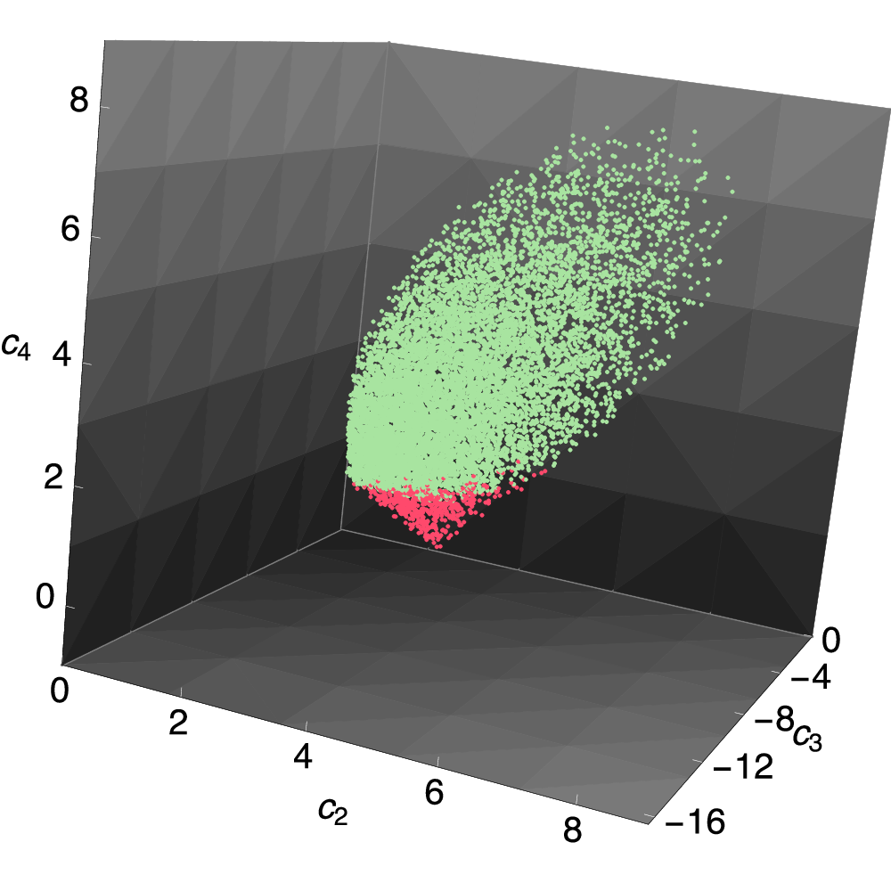
We begin by generating a large number of random points drawn uniformly in and then reject any point which does not satisfy criteria A-G. The surviving points are then saved. We plot the loci of these points on the - plane in Fig. 1.

Inspection of Fig. 1 reveals that the loci of points are nearly perfectly enveloped by the functions , with the exception of a small region prohibited by criterion E (). The envelope function may be derived starting from criteria A and G, as follows:
| (29) |
which may be re-arranged to
| (30) |
For the above to hold, then must be larger than one of the radicals but always less than the other, giving two possible sets of envelope functions. We define the first one as:
| (31) | |||
| (32) |
In Fig. 1, the pink line depicts , whilst the blue line depicts . This demonstrates that indeed our first guess for the form of the solution is correct. In principal though, we note that an alternative solution is .
From Fig. 1, one can see that there is a minimum allowed value and a maximum . The maximum coincides where the two envelope functions meet, meaning that , giving . The minimum value can be found by minimizing the lower envelope, which occurs at , corresponding to the minimum value of , or . This therefore provides two of the missing three LDC bounds we seek.
3.2 - plane
We may repeat this exercise in the - plane, and the resulting loci are shown in Fig. 2. As before, two lines appear to nearly perfectly envelope the loci of points, which can be derived starting from criteria A and G:

| (33) |
where the last line may now be re-expressed as
| (34) |
The above requires that is greater than one of the radicals but always less than the other. Therefore, we have two valid envelope functions and we define the first one as:
| (35) | |||
| (36) |
These two functions envelope the loci of points simulated earlier. This is apparent from Fig. 2, where the pink line denotes and the blue line . We plot the function from the upper-right intersection down to hitting the boundary condition of criterion F. Extending the line further back, shown as a dotted line, does not provide a physical bound on the points, although we note that only a very small fraction of points are excluded by doing so. In any case, the objective here is merely to determine the upper limit on .
We may use the function to find the maximum bound on . Maximizing the function by differentiation, we find the curve is maximized at , corresponding to . This provides the last limit needed to define the cuboid containing all loci as tightly as possible:
| (37) |
3.3 - plane
Although we have now derived all of the LDC bounds, for the sake of completeness we here consider envelope functions bounding the - plane, as shown in Fig. 3.

The pink and blue lines shown in Fig. 3 nearly perfectly envelope the loci of allowed points, with the exception of criterion E () truncating a small fraction of points. As before, these functions may be derived from the following:
| (38) |
which may be re-expressed as
| (39) |
Following the lines of argument used before, this provides the envelope functions:
| (40) | |||
| (41) |
We note that the two functions meet when , occurring at . However, criterion G truncates these functions, albeit only a small fraction of the envelope.
4 NUMERICAL TESTING OF THE CRITERIA
4.1 Overview
Starting from three physically imposed conditions for the intensity profile of a limb darkened star, we have derived seven criteria which bound the three LDCs parameterizing the Sing et al. (2009) limb-darkening law. In this section, we test the validity of these criteria in terms of (i) completeness and (ii) validity. We define these terms as follows:
-
Completeness: A fully complete set of criteria require that the loci of points for which the physical conditions are met also satisfy our seven criteria.
-
Validity: A fully valid set of criteria requires that that the loci of points which meet our seven criteria never break the two physical conditions.
These two tests can be thought of in the following way. Incomplete cases imply that our criteria are overly-conservative, cropping some parts of physically plausible parameter space. Invalid cases imply that our criteria are overly-optimistic, erroneously predicting that some parts of parameter space are physically plausible.
4.2 Completeness Tests
We perform our tests via numerical Monte Carlo simulation. We begin by drawing a uniform random point in the parameter space . The expected upper and lower bounds on these terms were calculated earlier in §3.2. We begin by using these bounds except that we use the original constraint rather than the modified criterion F. We then take this cuboid and double the lengths of each side such that we consider the ranges: , and . These adjustments are made to ensure that we explore the full range of physically allowed LDCs during this test.
A sample point is drawn from this cuboid and then tested as to whether the physical conditions I, II and III are met. In practice, we accomplish this by computing points along the functions and varying from to in equal, linear steps. For III we simply test if , since this condition only applies at the location . If the physical conditions are not met, then we generate a new trial point. If they are met, then we proceed to test if the analytic criteria A to G are satisfied for this accepted point.
In total, we repeat this process until accepted points are found, requiring simulations in total. Although the number of simulations may appear modest, we note that at each realization we must numerically compute the functions and at locations, which takes substantial computational overhead ( s per simulation).
We find that % of the accepted points also satisfy criteria A to G, or a completeness of %. This indicates that our seven criteria are slightly overly-conservative, cropping % of the physically permissible LDCs. If we use the unmodified versions of criteria F and G (see §2.6 and §2.7) and repeat the exercise, we find that % of the physically valid points satisfy the criteria. However, as discussed in §5, this now yields an asymmetric loci of allowed LDCs, impeding efforts to find an efficient sampling algorithm.
4.3 Validity Tests
In an analogous approach to the previous tests, we begin by drawing uniform random samples in as before, except that we know constrain the cuboid to the specific bounds derived in §3.2 (including ). We then test whether the seven analytic criteria are satisfied or not and if so consider the point to be accepted. We continue until accepted points are found, which we found required trials. Since we used the tightest bounding cuboid possible here, this reveals that the most efficient sampling possible without transforming the LDCs would be just under 1%. Whilst one could proceed in this way, applying an acceptance/rejection test at each realization, uniform sampling would reject over 99% of realizations, making such an approach highly inefficient.
We next test whether each of these accepted points satisfies the physical conditions I, II and III. As before, this is done by evaluating the functions and at evenly spaced locations.
From these tests, we find that 100% of the accepted points satisfy the physical criteria. Therefore, the seven criteria are fully valid and drawing a point which satisfies them is guaranteed to always satisfy the physical conditions I, II and III.
These tests therefore confirm that our criteria have a very high completeness and perfect validity. We therefore proceed with confidence that they provide a suitable set of constraints to evaluate the range of physically plausible LDCs.
5 TRANSFORMATIVE GEOMETRY
5.1 Overview
When plotted in the original parameter space (Fig. 4), the loci of physically allowed LDCs resemble a rotated, tilted ellipse of thin but finite width with a symmetric protrusion running along the semimajor axis. This complex morphology cannot be easily sampled from and if one wished to draw a set of LDCs from a uniform prior, there would be no alternative except to draw from the full cuboid and perform an acceptance/rejection test using our seven analytic criteria. As evident from Fig. 4, the volume of allowed points is much less than the bounding cuboid volume, meaning that such a procedure would be highly inefficient. Numerical tests reveal that the efficiency of such a procedure is just under 1%, making any algorithms using this method very wasteful.
We are therefore motivated to try and transform the geometry of the accepted loci of points into a more regular shape that we can sample from efficiently. We previously did this in the 2D case of quadratic limb darkening in Kipping (2013), but the transformative geometry required here is not only more complex but also includes an extra dimension.
5.2 Rescaled LDCs
We begin by noting that the envelope functions shown in Fig. 1-3 provide an excellent description for the bounding region of allowed LDCs. Despite some small exceptions, we are motivated to exclusively use these simple envelopes rather than the full criteria since i) they provide a nearly perfect description of the loci ii) the envelopes are symmetric functions derived from quadratic forms iii) all of the envelopes come from criteria A and G alone. In practice, criterion F is also necessary to remove a duplicate set of solutions.
We therefore proceed to only consider the region contained by criteria A, F and G, which we denote as the simplified region. This simplification means that the bounding cuboid is slightly modified to:
| (42) |
As a first transformation, we re-scale the axes into a unitary cube by the use of terms, defined as:
| (43) |
5.3 Righting the Allowed Region
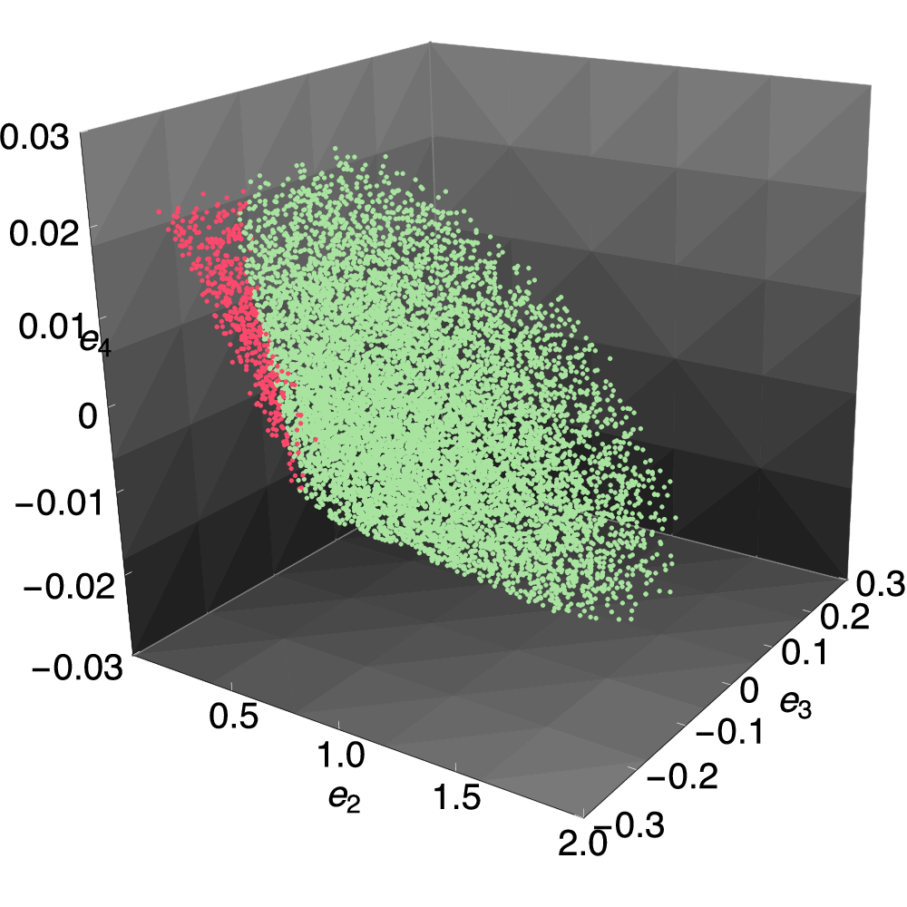
We next note that the loci (in parameter space) resembles an elliptic thin disk with the semimajor axis pointing along the unit vector . Further, the disk appears rotated about this unit vector, with respect to the axes of the reference frame. We decided to try to right the volume by performing a clockwise rotation of radians about the unit vector (). We then perform a further rotation which relocates the unit vector to (), followed by a third rotation relocating to (). The total rotation matrix applied is described by:
| (44) |
where
| (45) |
Applying these transformations gives a new-coordinate system of:
| (46) | ||||
| (47) | ||||
| (48) |
After visually inspecting the loci in this transformed parameter space (as shown in Fig. 5), we note that the allowed region now resembles a cone. Motivated by this observation, we proceed to transform this shape into a cone of symmetric proportions and with principal axes aligned to the transformed frame.
5.4 The Conal Region
As with the parameter space, our first step is to re-scale the axis into a cuboid with unit lengths, requiring us to first compute the extrema in space.
The extrema of occur when is maximized/minimized, as evident from Equation 48. This can be considered further by studying our earlier illustration in Fig. 2. This can be found by maximizing the function with respect to , which reveals the extrema is . We are therefore able to show that . This can also be achieved by maximizing/minimizing the expression using the additional constraints of criteria A, F and G. Repeating for the other terms we define a new boundary box of
| (49) | ||||
| (50) | ||||
| (51) |
We choose to re-scale the -parameter space into a unit vector cube via:
| (52) | ||||
| (53) | ||||
| (54) |
At this point, we now choose to rotate the conic section by radians in a clockwise sense around the -axis, so that the cone’s apex is located at the origin and the cone points along the -axis. We accomplish this using an additional change of variables:
| (55) | ||||
| (56) | ||||
| (57) |
where we have additionally normalized by a factor of to allow the loci to be symmetric on the - plane.
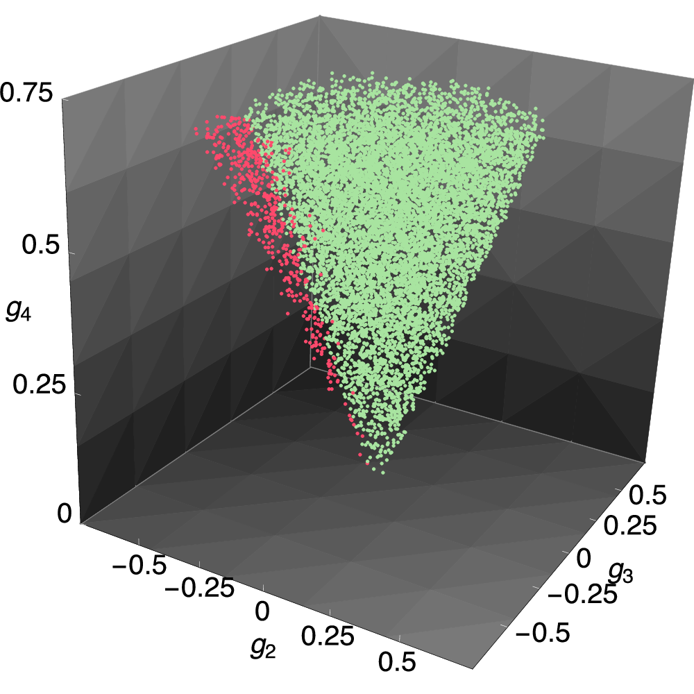
In this frame, our cone now has an apex at zero, with a height of and a radius of , as shown in Fig. 6. Writing out the terms relative to the original coefficients, we have
| (58) | ||||
| (59) | ||||
| (60) |
For which the inverse relations are
| (61) | ||||
| (62) | ||||
| (63) |
5.5 Sampling from the Conal Region
The samples shown in Fig. 6 appear consistent with points uniformly drawn from within the volume of a cone. We here describe the mathematical formalism by which one can compute such samples.
Samples may be drawn from a cone by first considering how to draw samples uniformly from within a circle. This well-known problem can be tackled by using polar coordinates and drawing a random polar angle in the range - rad and a random radius from a triangular distribution between and , where is the full radius. We now note that the radius varies as a function of height, , along the cone, such that . Finally, is drawn from a quadratic power-law distribution from to (the full height), since the area of a circle increases as . Drawing a random uniform variate for , and between 0 and 1, the polar angles, height and radius of a point uniformly drawn from within the cone may be expressed as
| (64) | ||||
| (65) | ||||
| (66) |
Converting these into Cartesian elements, we have
| (67) | ||||
| (68) | ||||
| (69) |
Or more explicitly:
| (70) | ||||
| (71) | ||||
| (72) |
We may also express the coefficients in terms of the uniform random variates, :
| (73) | ||||
| (74) | ||||
| (75) |
One may now work in the parameter space, drawing samples from within a unit cube (see Fig. 7) and then converting into a physically plausible set of LDCs using the above.
A unique set of inverse relations can be defined by use of an arc tangent accounting for the quadrant of the radical and the use of a floor function. We have written python and fortran code, called ldc3, to perform these functions, which is publicly available at this http.
5.6 Testing Samples Drawn from the Conal Region
We have provided no formal proof that the loci of points in -space is bound by a cone, nor do we explicitly claim so. We merely observe that the morphology of the loci most closely resembles this shape, from which it is possible to easily draw uniform samples. We here provide two simple tests demonstrating that sampling from the conal region provides an excellent set of physical LDCs.
First, we generated uniform random points from within the cone and tested whether they satisfied the physical conditions I, II and III. Using and , we find that 97.3% of the conal region is physical, or equivalently, points sampled from this region have a validity of 97.3%. Similarly, using the sample of valid points generated earlier in §4.3, we find a completeness of 94.4%. Therefore, points samples from the conal region crop % of the allowed parameter space.
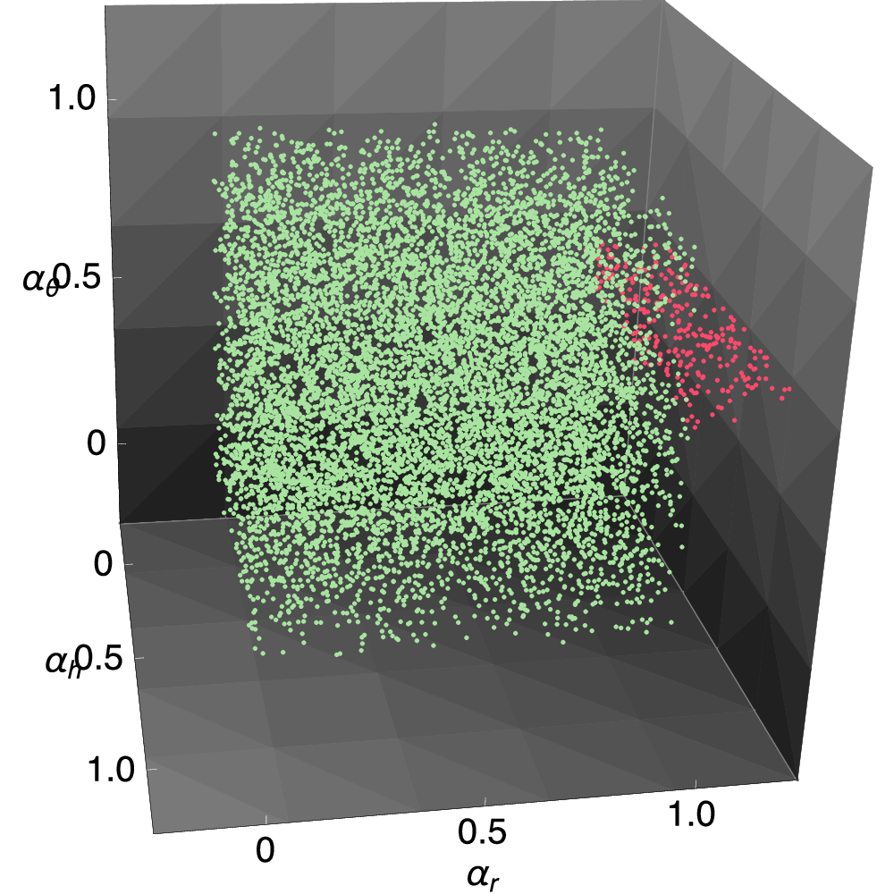
Aside from validity and completeness, we also consider the distribution of LDCs generated from sampling the conal region. We find that uniform samples from the -cone (or equivalently uniform points in the -cube) yield LDCs closely matching the distribution which would result from uniform sampling in -space with a simple acceptance/rejection of criteria A-G. This is evident in Fig. 8, where we compare the nearly identical distributions from these two approaches. One can also see in Fig. 7, that the valid samples plotted in -space (which were initially drawn uniformly in -space) provide an approximately uniform set of points within the unit cube.

6 DISCUSSION
In this work, we have presented a set of seven analytic criteria which may be used to assess the physicality of LDCs associated with the Sing et al. (2009) three-parameter non-linear limb-darkening law. We imposed simple conditions that the flux is everywhere positive, monotonically decreases from centre to limb and has a negative curl at the limb. Through numerical testing, we have shown that points naively sampled with a simple accept/reject algorithm applied to our criteria are always physically valid. Additionally, over 95% of the physically allowed loci of LDCs (found through brute force numerical exploration) satisfy the seven criteria, demonstrating a very high completeness. Using an unmodified set of criteria which retains the asymmetries present in the loci of allowed LDCs, the completeness is 100%.
Armed with these criteria, we have re-parametrized the LDCs such that the loci of allowed points morphologically resemble a regular geometric shape, specifically a cone. We have shown that uniformly sampling points from the conal region in the re-parametrized space yields physically plausible and uniformly distributed LDCs to high accuracy. Specifically, we find a validity of 97.4% and a completeness of 94.4%.
Sampling from the conal region may be achieved by drawing a uniform random variate in the transformed space , for which the relational expressions to the original LDCs are provided in Equation 75. We also provide public code (ldc3) in python and fortran to perform both the forward and inverse calculation between the parametrizations (this http).
Our work provides, for the first time, a practical and efficient framework for fitting astronomical data affected by limb-darkening with a law supporting three degrees of freedom. Until now, one had to limit oneself to efficient sampling of a two-parameter limb-darkening law (Kipping, 2013) and go without the major improvement in accuracy provided by a three-parameter law, such as that of Sing et al. (2009). Alternatively, one would have had to explore and marginalize over unphysical combinations of LDCs (which we estimate would occur for at least 99.9% of naively sampled points) or numerically test the physicality of each realization of LDCs (again with an overhead of rejecting the vast majority of points). In any case, we argue that our solution provides major advantages and enables the community to practically fit more complex limb-darkening profiles for the first time.
The only published grids of theoretical LDCs using the Sing et al. (2009) law comes from Sing (2010). With the Kepler bandpass, we find that 99.6% of the Sing (2010) tabulated points satisfy physical conditions I, II and III. Further more, 97.7% of these tabulated points reproduce an transformed LDC within the unit cube. These values again demonstrate that the parametrization can be practically used to explore the physically allowed LDCs. Since we now have an efficient strategy to fit LDCs, there is the potential to verify the predictions made from theoretical models by the study of high signal-to-noise transits in the future.
In some applications, having “only” % of the LDCs being physically valid may be insufficient and one may wish to ensure 100% validity. Since the seven analytic criteria guarantee 100% validity, one may draw a set of LDCs using the parametrization and then test if this realization satisfies the seven criteria. In practice, criteria B and D are never violated by points sampled from the conal region and thus it is only necessary to test five criteria. This approach enables a guaranteed physically plausible set of LDCs at minimal computational expense. To aid the community, our code ldc3 can perform this test (this http).
Whilst the quadratic law (and other two parameter laws) will likely remain suitable for many studies, the analysis of high precision data increasingly demands a more sophisticated treatment of limb-darkening to avoid this issue becoming a bottleneck in obtainable accuracy (Epinoza & Jordán, 2015). By freely fitting high-precision data with our parametrization of the Sing et al. (2009) limb-darkening, one can have greater confidence that the parameters of interest are marginalized exclusively over the physically plausible parameter space and limb-darkening is modelled in a manner more consistent with simulations from modern stellar atmosphere models. We also note that informative priors on our parametrization may be used as well, in cases where one has strong belief in the results of stellar atmosphere models and the star is well-characterized already, or alternatively from previous posteriors derived from freely fitting the LDCs. For either informative or uninformative sampling, the parametrization offers an efficient and physically sound pathway to exploring parameter space when modelling limb-darkening under the three-parameter law.
Acknowledgements
DMK acknowledges support from the CfA Menzel fellowship programme and thanks the anonymous reviewer for their helpful comments.
References
- Aufdenberg et al. (2005) Aufdenberg, J. P., Ludwig, H.-G. & Kervella, P., 2005, ApJ, 633, 424
- Bigot et al. (2006) Bigot, L., Kervella, P., Thévenin, F. & Ségransan, D., 2006, A&A, 446, 635
- Claret (2000) Claret, A., 2000, A&A, 363, 1081
- Csizmadia et al. (2013) Csizmadia, Sz., Pasternacki, Th., Dreyer, C., Cabrera, J., Erikson, A. & Rauer, H., 2013, A&A, 549, 9
- Díaz-Cordovéz et al. (1995) Díaz-Cordovéz, J., Claret, A. & Giménez, A., 1995, A&AS, 110, 329
- Epinoza & Jordán (2015) Epinoza, N. & Jordán, A., 2015, MNRAS, 450, 1879
- Giménez (2006) Giménez, A., 2006, A&A, 450, 1231
- Van Hamme (1993) Van Hamme, W., 1993, AJ, 106, 2096
- Howarth (2011) Howarth, I. D., 2011, MNRAS, 418, 1165
- Kipping & Bakos (2011a) Kipping, D. M. & Bakos, G. A., 2011a, ApJ, 730, 50
- Kipping & Bakos (2011b) Kipping, D. M. & Bakos, G. A., 2011b, ApJ, 733, 36
- Kipping (2012) Kipping, D. M., 2012, MNRAS, 427, 2487
- Kipping (2013) Kipping, D. M., 2013, MNRAS, 435, 2152
- Kopal (1950) Kopal, Z., 1950, Harvard Col. Obs. Circ., 454, 1
- Knutson et al. (2007) Knutson, H. A., Charbonneau, D., Noyes, R. W., Brown, T. M. & Gilliland, R. L., 2007, ApJ, 655, 564
- Kreidberg et al. (2014) Kreidberg, L. Bean, J. L., Désert, J.-M. and 7 other authors, 2014, Nature, 505, 69
- Magic et al. (2015) Magic, Z., Chiavassa, A., Collet, R. & Asplund, M., 2015, A&A, 573, 90
- Mandel & Agol (2002) Mandel, K. & Agol, E., 2002, ApJ, 580, 171
- Morris & Naftilan (1993) Morris, S. L. & Naftilan, S. A., 1993, ApJ, 419, 344
- Neckel & Labs (1994) Neckel, H. & Labs, D., 1994, Sol. Phys., 153, 91
- Schlawin et al. (2010) Schlawin, E., Agol, E., Walkowicz, L. M., Covey, K. & Lloyd, J. P., 2010, ApJ, 722, L75
- Sing et al. (2009) Sing, D. K., Désert, J.-M., Lecavelier Des Etangs, A., Ballester, G. E., Vidal-Madjar, A., Parmentier, V., Hebrard, G. & Henry, G. W., 2009, A&A, 505, 891
- Sing (2010) Sing, D. K., 2010, A&A, 510, 21
- Witt (1995) Witt, J. J., 1995, ApJ, 449, 42
- Zub et al. (2011) Zub, M. et al., 2011, A&A, 525, 15