The magnetized effective QCD phase diagram

The behavior of strongly interacting matter in presence of magnetic fields has become a subject of increasing interest over the past few years. This interest has been sparked by recent lattice QCD (LQCD) results showing that the transition temperature with 2 + 1 quark flavors decreases with increasing magnetic field and that the strength of the condensate decreases for temperatures close and above the phase transition [1, 2, 3, 4]. This behavior has been dubbed inverse magnetic catalysis, and it has been the center of attention in a large number of model-dependent analyses [5, 6, 7, 8, 9, 10, 11, 12, 13, 14, 15, 16]. For recent reviews see Refs. [17, 18]. In general terms, it seems that inverse magnetic catalysis is not obtained in mean field approaches describing the thermal environment [19, 20, 21, 22, 23, 24], nor when calculations beyond mean field do not include magnetic effects on the coupling constants [25].

The novel feature implemented in effective models, able to account self-consistently for inverse magnetic catalysis, is the decrease of the coupling constants with increasing field strength obtained from the model itself [26, 27] without resorting to ad hoc parametrizations. This has been achieved within the Abelian Higgs model and the linear sigma model coupled to quarks (LSMq). This behavior is made possible by accounting for the screening properties of the plasma, which have been recently formulated consistently for theories with spontaneous symmetry breaking [25]. This results in a formalism beyond the mean field approximation [26]. Screening is also important to obtain a decrease of the coupling constant with the magnetic field strength in QCD in the Hard Thermal Loop approximation [28]. It has also been shown, by means of a QCD sum rules analysis at zero temperature, that both, the threshold energy for the onset of the continuum in the quark vector current spectral density (a phenomenological parameter that signals the onset of deconfinement) and the gluon condensate increase with increasing magnetic field, as expected [29].

Recently, the LSMq has been also used to explore the phase diagram without magnetic fields [30]. It was found that there are values for the model couplings that allow locating a critical end point (CEP) in the region where lattice inspired calculations find it [31]. Since the LSMq does not exhibit confinement, this behavior is attributed to the proper treatment of plasma screening, instead of to the existence of a given confinement length scale [32].

A pertinent question is whether the above description in the presence of a magnetic field can be used to study how such CEP changes with the field intensity. Recent LQCD calculations [33] show that for very strong magnetic fields, inverse magnetic catalysis prevails and the phase transition becomes first order at asymptotically large values of the magnetic field for vanishing quark chemical potential $\mu$. A similar behavior is obtained in the Nambu Jona-Lasinio model if one includes a magnetic field dependence of the critical temperature in agreement with LQCD [34].

In this paper we use the LSMq to explore the consequences of a proper handling of the plasma screening properties in the description of the magnetized effective QCD phase diagram. We show that when including self-consistently magnetic field effects in the calculation of both the effective potential as well as on the thermo-magnetic dependence of the coupling constants, the CEP’s location moves toward smaller values of the critical quark chemical potential, and larger values of the critical temperature. In addition, above a certain value of the field strength the CEP moves to towards the $T$-axis. We argue that this behavior can be understood on general grounds, as the magnetic field produces a dimension reduction, whereby virtual charged particles from the vacuum are effectively constrained to occupy Landau levels, thus restricting their motion to a plane. This makes these particles to lay closer to each other on average, thus reducing the interaction strength for strongly coupled theories. This situation takes place regardless of how weak the external field is.

The paper is organized as follows: In Sec. II we recall the basic features of the linear sigma model with quarks, and in the presence of a magnetic field. Next, we write the effective potential at finite temperature and quark chemical potential, including all the degrees of freedom of the model. In Sec. III we find the thermo-magnetic corrections to the boson self-coupling and to the coupling between fermions and bosons. In Sec. IV we find the effects of the thermo-magnetic dependence of the couplings on the critical temperature $T_{c}$ for chiral symmetry restoration transition. We find that $T_{c}$ is a decreasing function of the magnetic field for any value of $\mu$. We also study the magnetized effective QCD phase diagram and in particular find how the CEP’s location changes with the field strength. We finally summarize and conclude in Sec. V. In the appendix we describe the computation of the thermo-magnetic corrections to the couplings, and to the temperature and density dependence of the fermion thermal mass.

The Lagrangian of the sigma model, including quark degrees of freedom, is given by

where $\psi$ is an SU(2) isospin doublet, $\vec{\pi}=(\pi_{1},\pi_{2},\pi_{3})$ is an isospin triplet and $\sigma$ is an isospin singlet, with

is the covariant derivative. $A^{\mu}$ is the vector potential corresponding to an external magnetic field directed along the $\hat{z}$ axis. In the symmetric gauge it is given by

where $q$ is the particle’s electric charge. $A^{\mu}$ satisfies the gauge condition $\partial_{\mu}A^{\mu}=0$. The gauge field couples only to the charged pion combinations, namely

The neutral pion is taken as the third component of the pion isovector, $\pi^{0}=\pi_{3}$. The gauge field is taken as classical and thus we do not consider loops involving the propagator of the gauge field in internal lines. The squared mass parameter $a^{2}$ and the self-coupling $\lambda$ and $g$ are taken to be positive.

To allow for spontaneous symmetry breaking, we let the $\sigma$ field to develop a vacuum expectation value $v$

This vacuum expectation value can later be identified as the order parameter of the theory. After this shift, the Lagrangian can be rewritten as

where ${\mathcal{L}}_{I}^{b}$ and ${\mathcal{L}}_{I}^{f}$ are given by

The terms given in Eq. (7) describe the interactions among the fields $\sigma$, $\vec{\pi}$ and $\psi$, after symmetry breaking. From Eq. (6) one can see that the $\sigma$, the three pions and the quarks have masses given, respectively, by

Using Schwinger’s proper-time method, the expression for the one-loop effective potential for one boson field with squared mass $m_{b}^{2}$ and absolute value of its charge $q_{b}$ at finite temperature $T$ in the presence of a constant magnetic field can be written as

where $\omega_{n}=2n\pi T$ are boson Matsubara frequencies. Similarly, the expression for the one-loop effective potential for one fermion field with mass $m_{f}$ and absolute value of its charge $q_{f}$ at finite temperature $T$ and chemical potential $\mu$, in the presence of a constant magnetic field can be written as

where $\tilde{\omega}_{n}=(2n+1)\pi T$ are fermion Matsubara frequencies. The sum over the index $r$ corresponds to the two possible spin orientations along the magnetic field direction.

Including the $v$-independent terms, choosing the renormalization scale as $\tilde{\mu}=e^{-1/2}a$ and after mass and charge renormalization, the thermo-magnetic effective potential in the small to intermediate field regime, in a high temperature expansion can be written as

where $\psi^{0}(x)$ is the digamma function, $Li_{n}$ is the polylogarithm function of order $n$, $q$ is the absolute value of the charged pion charge ($q=1$), $q_{u}=2/3$, and $q_{d}=1/3$ are the absolute values of the up- and down-quarks, respectively, $\gamma_{E}$ is the Euler’s gamma, $N_{f}=2$ is the number of light-quark flavors, and $N_{c}=3$ is the number of colors. In order to obtain the leading magnetic field contribution of Eq. (11) we use the Euler-MacLaurin expansion [25] in Eqs. (9) and (10).

Though we take the quark masses as equal, the notation emphasizes that the effective potential is evaluated after accounting for the different quark charges. We have introduced the leading temperature plasma screening effects for the boson masses squared, encoded in the boson self-energy $\Pi$. The leading contribution for the boson self-energy in a high temperature expansion, and at finite $\mu$ is given by [30]

For the Hurwitz zeta function $\zeta(-1/2,z)$ in Eq. (11) to be real, one needs

a condition that arises from requiring that the second argument of the Hurwitz zeta function satisfies $z>0$, even for the lowest value of $m_{b}^{2}$ which is obtained for $v=0$. Furthermore, for the large $T$ expansion to be valid, one also requires

The conditions expressed in Eqs. (13) and (14) provide the limits of applicability of the high temperature expansion of the effective potential in Eq. (11).

We now compute the one-loop correction to the coupling $\lambda$, including thermal and magnetic effects. Figure 1 shows the Feynman diagrams that contribute to this correction. Columns (a), (b), (c), (d), (e) and (f) contribute, respectively, to the correction to the $\sigma^{4}$, $(\pi^{0})^{4}$, $(\pi^{+})^{2}(\pi^{-})^{2}$, $\sigma^{2}\pi^{+}\pi^{-}$, $(\pi^{0})^{2}\pi^{+}\pi^{-}$ and $\sigma^{2}(\pi^{0})^{2}$ terms of the interaction Lagrangian in Eq. (7), respectively. Since each of these corrections lead to the same result, we concentrate on the diagrams in column (a). Each of the three diagrams involves two propagators of the same boson. For the first two diagrams the intermediate bosons are neutral and for the third one the intermediate bosons are charged.

The explicit computation has been performed in Ref. [27]. This involves the use of the weak field expansion of the charged boson Schwinger proper-time propagator for the intermediate charged particles and its corresponding $qB\rightarrow 0$ limit for the intermediate neutral bosons. Since the analysis of Ref. [27] was carried out in the very high temperature case, the four-boson vertex correction was evaluated in the infrared limit, namely $P_{i}=(0,{\mbox{\bf{p}}}\rightarrow 0)$, where $P_{i}$ are the momenta of each of the four external legs. However, for the present analysis, where $T$ is close to $T_{c}$ a more appropriate treatment is to evaluate the vertex function at the typical energy of the external particles. This corresponds to the static limit, namely $P_{i}=(\Pi,{\mbox{\bf{p}}}=0)$, where $\Pi$ is given by Eq. (12) and represents the purely thermal (and density) component of the boson mass. In the appendix, we explicitly reproduce such calculation, evaluating the vertex function in the static limit. Notice that $\lambda_{\mbox{\small{eff}}}$ depends on $v$ through the dependence on the boson masses. We further consider the approximation where $\lambda_{\mbox{\small{eff}}}$ is evaluated at $v=0$ since we are pursuing the effect on the critical temperature, which is the temperature where the curvature of the effective potential at $v=0$ vanishes.

Next we turn to the calculation of the thermo-magnetic correction of the coupling $g$. Figure 2 shows the Feynman diagrams that contribute to this correction. We are interested in computing an effective value for this coupling, $g_{\mbox{\small{eff}}}$, as well as for $v=0$, in the same manner done for $\lambda_{\mbox{\small{eff}}}$. Columns (a), (b) and (c) contribute to the correction to the quark-$\sigma$, quark-$\pi^{0}$ and quark-$\pi^{\pm}$ terms of the interaction Lagrangian of Eq. (7), respectively. Since each of these corrections leads to the same result, we concentrate on the diagrams in column (a). Notice that for $v=0$ in Eq. (8), the masses of the $\sigma$ and the $\pi^{0}$ become degenerate. Hence, the middle and bottom diagrams in column (a) of Fig. 2 cancel out, since they contribute with opposite signs. This also happens with the two bottom diagrams in columns (b) and (c).

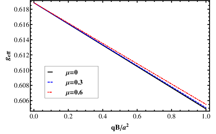
The explicit computation is carried out in the weak field limit of the charged boson and fermion Schwinger proper-time propagators. The calculation was done in Ref. [27] considering only terms of ${\mathcal{O}}$ $(qB)^{2}$ after taking the average over spins. We have repeated the calculation and realized that the contribution ${\mathcal{O}}$ $(qB)$ does not vanish. This is because such spin average is not needed, as we are not considering a decay process, but rather a vertex function. We have also evaluated $g_{\mbox{\small{eff}}}$ in the static limit $P_{i}=(m_{f}^{\mbox{\tiny{them}}},{\mbox{\bf{p}}}=0)$ where $P_{i}$ are the momenta of the quark and antiquark and $m_{f}^{\mbox{\tiny{them}}}$ is the fermion thermal (and density)-dependent mass, which we compute in the appendix and whose square is given explicitly by

To fix the bare values of the couplings $\lambda$, $g$ and $a$ appropriate for the description of the phase transition, we notice that the boson masses are modified when considering the thermal effects, since they acquire a thermal component. For $\mu=0$ they become

At the phase transition, the curvature of the effective potential vanishes for $v=0$. Since the boson masses are proportional to this curvature, these also vanish at $v=0$. In this case, and from any of Eqs. (), we then obtain a relation between $T_{c}^{0}$ and the model parameters at the critical temperature with $\mu=0$

Furthermore, we can fix the value of $a$ by noting from Eqs. (8) that the vacuum boson masses satisfy

Since the effective potential is written as an expansion in powers of $a/T$ we need that this ratio satisfies $a/T<1$. From Eqs. (17) and (18) the coupling constants are proportional to $m_{\sigma}$ which, from the above conditions, restricts the analysis to considering not too large values of $m_{\sigma}$ as well as not too small values of $T_{c}^{0}$. Since the purpose of this work is not to pursue a precise determination of the couplings but instead to call attention to the fact that the proper treatment of screening effects allows the linear sigma model to provide solutions for the CEP even at finite values of $\mu$, we consider small values for $m_{\sigma}$. Given that $\sigma$ is anyhow a broad resonance, in order to satisfy the above requirements let us take for definitiveness $m_{\sigma}=300$ MeV. namely, close to the two-pion threshold. For $T_{c}^{0}$ with two light quark flavors we take $T_{c}^{0}=172$ MeV [35]. Thus, $a/T_{c}^{0}=0.77$. Equation (17) provides a relation between $\lambda$ and $g$. A possible solution consistent with the above requirements is given by $\lambda=0.4$, $g=0.63$.

Figure 3 shows the behavior of the effective boson coupling $\lambda_{\mbox{\small{eff}}}$ evaluated using $T=180$ MeV, as a function of magnetic field strength for different values of $\mu$. The considered temperature is slightly larger that $T_{c}^{0}$. Note that $\lambda_{\mbox{\small{eff}}}$ is a monotonically decreasing function of $qB$ and that the decrease is larger for larger values of $\mu$.

Figure 4 shows the behavior of $g_{\mbox{\small{eff}}}$ as a function of $qB$ evaluated also using $T=180$ MeV with $\lambda=0.4$, $g=0.63$ for three different values of $\mu$. Note that $g_{\mbox{\small{eff}}}$ is also a monotonically decreasing function of $qB$. However, the decrease is less pronounced for larger values of $\mu$. Note that the $\mu$-dependence of the effective coupling comes from its dependence on $m_{f}^{\mbox{\tiny{them}}}$.

We now study the effect of the thermo-magnetic corrections to the couplings on the critical temperature. For a given value of the magnetic field, and for a second order phase transition, the critical temperature is determined after setting to zero the second derivative of the effective potential at $v=0$ in Eq. (11). When the phase transition becomes first order, the critical temperature is computed by determining the temperature where a secondary minimum for $v\neq 0$ is degenerate with a minimum at $v=0$. Figure 5 shows the critical temperature as a function of field strength, for different values of $\mu$, and for the bare values $\lambda=0.4$, $g=0.63$. Note that in all cases the critical temperature is a decreasing function of the field strength.

On the contrary when the calculation is performed without including the thermo-magnetic modification to the couplings, the critical temperature turns out to be an increasing function of the field strength. This is shown in Fig. 6 where we plot the critical temperature as a function of $qB$ for different values of $\mu$ with the bare values of the couplings $\lambda=0.4$, $g=0.63$. This behavior shows that the thermo-magnetic corrections to the couplings are crucial to obtain inverse magnetic catalysis.

We now turn to describe the phase diagram in the temperature quark chemical potential plane. Figure 7 shows the phase diagram obtained for the bare couplings $\lambda=0.4$, $g=0.63$ for different values of the magnetic field strength. The thermo-magnetic corrections enter the analysis both in the effective potential of Eq. (11), and in the effective couplings. Notice that as the field intensity increases, the CEP moves toward lower values of the critical quark chemical potential, and to larger values of the critical temperature and in this case, it reaches the $T$-axis. However, since our analysis is carried out in the weak field limit $qB/T^{2}<1$, we can only say that there is a tendency for the CEP to eventually reach the $T$-axis large values of the field strength.

To see the effect of a change of parameters we now explore the case where the ratio $a/T_{c}^{0}$ appearing in Eq. (17) changes. We take $a/T_{c}^{0}=0.66$ which is obtained maintaining $m_{\sigma}=300$ MeV and increasing the value of $T_{c}^{0}$ to $T_{c}^{0}=200$ MeV. With this ratio, a possible solution to Eq. (17) for the bare values of the couplings is given by $\lambda=0.36$, $g=0.51$. Figure 8 shows the phase diagram thus obtained. Notice that the CEP for $qB=0$ happens for values of $T_{c}^{\mbox{\tiny{CEP}}}$ and $\mu_{c}^{\mbox{\tiny{CEP}}}$ slightly smaller and larger, respectively, than for the corresponding values in Fig. 7. When the magnetic field intensity increases the CEP also moves toward lower values of the critical quark chemical potential and larger values of the critical temperature but this time, for the largest value of $qB$ considered, the CEP does not reach the $T$-axis. Nevertheless we observe a tendency for the CEP to eventually reach the $T$-axis for larger values of $qB$ that can not be studied within the present small field approach.

In conclusion, we have shown that working in the LSMq in the presence of magnetic fields, it is possible to obtain values for the couplings that allow to locate a CEP that for $qB=0$, lays in the region found by mathematical extensions of lattice analyses. The analysis is done from the effective potential computed in the presence of a weak magnetic field and accounting for the plasma screening effects. Since the LSMq does not have confinement, we attribute the CEP’s location to the adequate description of the plasma screening properties. Screening is included into the calculation in two manners:

First, in the effective potential through the boson’s self-energy and second in the thermo-magnetic corrections of the couplings. We have shown that this last correction is crucial to obtain inverse magnetic catalysis. To define the allowed range for the bare coupling constants we observe that the thermal boson masses vanish at the phase transition for $\mu=0$. This condition determines a relation between the model parameters which can be put in quantitative terms from knowledge of $T_{c}^{0}$ and $a$. The first can be obtained from lattice results and the second from the vacuum boson masses. Since the model is computed in the high temperature limit, we are limited to consider ratios of the parameter $a/T_{c}^{0}$ a bit off their usual values. Nevertheless, the model shows in quantative terms that the CEP moves toward lower values of the critical quark chemical potential and larger values of the critical temperature as the field intensity increases and that there is a tendency for the CEP to eventually reach the $T$-axis for a larger value of the field strength.

The overall features of the phase diagram can be understood in general terms when we recall that the magnetic field produces a dimension reduction whereby the virtual charged particles that make up the vacuum are effectively constrained to occupy Landau levels which, in semiclassical terms, implies that their motion is restricted to planes. This produces that these particles lay on average closer to each other. Since as a function of the field intensity we have shown that the strength of the interaction is reduced, and that this happens no matter how weak the external field may be, we infer that a similar effect is taking place in QCD where due to asymptotic freedom, the strength of the interaction gets reduced as the virtual particles get closer to each other. This weakening of the interaction with proximity between the virtual particles that make up the vacuum should manifest itself as well in the weakening of the quark condensate with the field strength, as is also observed in lattice QCD around the critical temperature. We believe this description will play an important role in the interpretation of the lattice QCD results for the behavior of the critical temperature and the quark condensate with the field intensity as well as in determining the location of the CEP in QCD with and without magnetic fields.

This work has been supported in part by DGAPA-UNAM (Mexico) under grant number PAPIIT-IN101515, CONACyT (Mexico) under grant number 128534, FONDECYT (Chile) under grant numbers 1130056 and 1120770, and 21110295, NRF (South Africa), and the Harry Oppenheimer Memorial Foundation (South Africa). R. Z. acknowledges support from CONICYT under Grant No. 21110295.

References

• [1] G. S. Bali, F. Bruckmann, G. Endrodi, Z. Fodor, S. D. Katz, S. Krieg, A. Schafer, and K. K. Szabo, J. High Energy Phys. 02, 044 (2012).
• [2] G. S. Bali, F. Bruckmann, G. Endrödi, Z. Fodor, S. D. Katz and A. Schafer, Phys. Rev. D 86, 071502 (2012).
• [3] G. S. Bali, F. Bruckmann, G. Endrödi, S. D. Katz and A. Schafer, J. High Energy Phys. 1408 (2014) 177.
• [4] G. S. Bali, F. Bruckmann, G. Endrödi, Z. Fodor, S. D. Katz, and A. Schäfer, Phys. Rev. D 86, 071502 (2012).
• [5] E. S. Fraga, J. Noronha and L. F. Palhares, Phys. Rev. D 87, 114014 (2013).
• [6] F. Bruckmann, G. Endrodi and T. G. Kovacs, J. High Energy Phys. 1304, 112 (2013).
• [7] M. Ferreira, P. Costa, D. P. Menezes, C. Providencia and N. N. Scoccola, Phys. Rev. D89, 016002 (2014).
• [8] K. Fukushima and Y. Hidaka, Phys. Rev. Lett. 110, 031601 (2013).
• [9] N. Mueller and J. M. Pawlowski, Phys. Rev. D 91, 11, 116010 (2015).
• [10] J. O. Andersen and A. Tranberg, J. High Energy Phys. 1208, 002 (2012); J. O. Andersen, W. R. Naylor, and A. Tranberg, J. High Energy Phys. 1404, 187 (2014).
• [11] J. Braun, W. A. Mian, S. Rechenberger, arXiv:1412.6025 [hep-ph].
• [12] G. S. Bali, F. Bruckmann, G. Endrodi, F. Gruber, A. Schaefer, J. High Energy Phys. 1304, 130 (2013).
• [13] E. J. Ferrer, V. de la Incera, X. J. Wen, Phys. Rev. D 91, 054006 (2015).
• [14] Sh. Fayazbakhsh and N. Sadooghi, Phys. Rev. D 90, 105030 (2014).
• [15] R. L. S. Farias, K. P. Gomes, G. Krein and M. B. Pinto, Phys. Rev. C 90, 025203 (2014).
• [16] M. Ferreira, P. Costa, O. Lourenço, T. Frederico, C. Providência, Phys. Rev. D 89, 116011 (2014).
• [17] J. O. Andersen, W. R. Naylor, A. Tranberg, arXiv:1411.7176 [hep-ph].
• [18] V. A. Miransky, I. A. Shovkovy, Phys. Rept. 576, 1-209 (2015).
• [19] J. O. Andersen, W. R. Naylor, A. Tranberg, J. High Energy Phys. 1502, 042 (2015).
• [20] E. S. Fraga and A. J. Mizher, Phys. Rev. D 78, 025016 (2008).
• [21] M. Loewe, C. Villavicencio, R. Zamora, Phys. Rev. D 89, 016004 (2014).
• [22] N. O. Agasian and S. M. Fedorov, Phys. Lett. B 663, 445 (2008).
• [23] A. J. Mizher, M. N. Chernodub and E. S. Fraga, Phys. Rev. D 82, 105016 (2010).
• [24] E. S. Fraga, B. W. Mintz, J. Schaffner-Bielich, Phys. Lett. B 731, 154 (2014).
• [25] A. Ayala, L. A. Hernández, A. J. Mizher, J. C. Rojas, C. Villavicencio, Phys. Rev. D 89, 116017 (2014).
• [26] A. Ayala, M. Loewe, A. J. Mizher, R. Zamora, Phys. Rev. D 90, 036001 (2014).
• [27] A. Ayala, M. Loewe and R. Zamora, Phys. Rev. D 91, 016002 (2015).
• [28] A. Ayala, J.J. Cobos-Martinez, M. Loewe, M. E. Tejeda-Yeomans, and R. Zamora, Phys. Rev. D 91, 016007 (2015).
• [29] A. Ayala, C.A. Dominguez, L.A. Hernandez, M. Loewe, J. C. Rojas, C. Villavicencio, Phys. Rev. D 92, 1, 016006 (2015).
• [30] A. Ayala, A. Bashir, J. J. Cobos-Martínez, S. Hernández, A. Raya, Nucl. Phys. B 897, 77-86 (2015).
• [31] S. Sharma, Adv. High Energy Phys. 2013, 452978 (2013).
• [32] S.-x. Qin, L. Chang, H. Chen, Y.-x. Liu and C. D. Roberts, Phys. Rev. Lett. 106, 172301 (2011).
• [33] G. Endrödi, arXiv:1504.08280 [hep-lat].
• [34] P. Costa, M. Ferreira, D. P. Menezes, J. Moreira and C. Providência, arXiv:1508.07870 [hep-ph]; M. Ferreira, P. Costa, C. Providência, arXiv:1509.01181 [hep].
• [35] Y. Maezawa, S. Aoki, S. Ejiri, T. Hatsuda, N. Ishii, K. Kanaya, N. Ukita, J. Phys. G 34, S651 (2007).
• [36] D. Bedingham, arXiv:hep-ph/0011012 (2000).
• [37] B. R. Paris, Proc. R. Soc. A 461, 297 (2004).
• [38] L. Dolan and R. Jackiw, Phys. Rev. D 9, 3320 (1974).
• [39] J. I. Kapusta, Thermal Field Theory, Cambridge University Press (1989).