Geometric Bijections Between Spanning Trees and Break Divisors

Unless otherwise specified, all graphs in this paper are assumed to be finite and connected, possibly with parallel edges but without any loops; the term cycle will refer to a simple cycle. We use $n$ and $m$ to denote the number of vertices and edges of a graph, respectively. The Laplacian matrix $\Delta$ of a graph is the $n\times n$ matrix defined as $D-A$, where $D$ is a diagonal matrix with the $(i,i)$-entry being the degree of the vertex $v_{i}$, and $A$ is the adjacency matrix of $G$ with the $(i,j)$-entry being the number of edges between $v_{i}$ and $v_{j}$ for $i\neq j$ and 0 for $i=j$.

A divisor on a graph $G=(V,E)$ is a function $D:V\rightarrow\mathbb{Z}$. The set of all divisors on $G$ is denoted by $\operatorname{Div}(G)$; it has a natural group structure as the free abelian group generated by $V$. The degree $\deg(D)$ of a divisor $D$ is $\sum_{v\in V}D(v)$, and the set of all divisors of degree $k$ is denoted by $\operatorname{Div}^{k}(G)$. Identifying divisors with vectors in $\mathbb{Z}^{n}$, we say a divisor is principal if it is equal to $\Delta{\bf u}$ for some integral vector ${\bf u}$. The set of all principal divisors is denoted by $\operatorname{Prin}(G)$. $\operatorname{Prin}(G)$ is a subgroup of $\operatorname{Div}^{0}(G)$ and the quotient group $\operatorname{Div}^{0}(G)/\operatorname{Prin}(G)$ is the (degree 0) Picard group $\operatorname{Pic}^{0}(G)$ of $G$; the Picard group of a graph is also known as the Jacobian, the sandpile group or the critical group of the graph in other literature. More generally we say two divisors $D,D^{\prime}$ are linearly equivalent, denoted $D\sim D^{\prime}$, if $D-D^{\prime}\in\operatorname{Prin}(G)$. We denote by $\operatorname{Pic}^{k}(G)$ the set $\operatorname{Div}^{k}(G)/\!\!\sim$. It is easy to see that $\operatorname{Pic}^{k}(G)$ and $\operatorname{Pic}^{0}(G)$ differ only by a degree $k$ translating element.

Given a divisor $D$, we often say there are $D(v)$ chips at vertex $v$, and we can construct a divisor on $G$ by adding or removing chips on vertices in various ways. The concept of linear equivalence can be captured by the chip-firing game on $G$, see [7] for its usage in the Riemann-Roch theory on graphs and [30] for a brief overview of chip-firing in other parts of mathematics.

A spanning tree of $G$ is a connected spanning subgraph of $G$ with no cycles. Denote by $g:=m-n+1$ the genus (or cyclomatic number) of $G$, which is the number of edges outside any spanning tree of $G$²² 2 We clarify that $g$ is not the topological genus of $G$ as in the usual topological graph theory sense.. It is known that the Picard group has the same cardinality as the set of spanning trees $S(G)$ of a graph [2, 17]. A degree $g$ divisor is called an (integral) break divisor if it can be obtained from the following procedure: choose a spanning tree $T$ of $G$, and for every edge $f\not\in T$, pick an orientation of $f$ and add a chip at the head of $f$. In general, different choices of spanning trees and orientations can produce the same break divisor. It is proven in [1, Theorem 1.3] that break divisors form a set of representatives for the divisor classes in $\operatorname{Pic}^{g}(G)$. In particular, the number of break divisors is equal to the number of spanning trees of $G$.

A metric graph $\Gamma$ (or an abstract tropical curve) is a compact connected metric space such that every point has a neighborhood isometric to a star-shaped set. Every metric graph can be constructed in the following way: start with a weighted graph $(G=(V,E),w:E\rightarrow\mathbb{R}_{>0})$, associate with each edge $e$ a closed line segment $L_{e}$ of length $w(e)$, and identify the endpoints of the $L_{e}$’s according to the graph structure in the obvious way. A (weighted) graph $G$ that yields a metric graph $\Gamma$ is said to be a model of $\Gamma$. The genus of $\Gamma$ is the genus of any model of $\Gamma$. See [5] for details. For simplicity, we assume all graphs we consider have uniform edge weights 1, though most geometric propositions in this paper remain valid for the general case.

Metric graphs have an analogous theory of divisors as graphs; we refer the reader to [1] for details and only explain the most relevant notions here. A divisor on $\Gamma$ is an element of the free abelian group generated by $\Gamma$; equivalently, it is a function $D:\Gamma\rightarrow\mathbb{Z}$ of finite support. A divisor $D=(p_{1})+(p_{2})+\ldots+(p_{g})$ is a break divisor if there is a model $G$ for $\Gamma$ and an edge $e_{i}$ of $G$ for each $p_{i}$ such that $p_{i}\in L_{e_{i}}\subset\Gamma$ (by the definition of $L_{e_{i}}$, $p_{i}$ can be on the endpoints of $e_{i}$), and $G-\{e_{1},\ldots,e_{g}\}$ is a spanning tree of $G$. As in the case of graphs, break divisors on $\Gamma$ form a set of representatives for the equivalence classes in $\operatorname{Pic}^{g}(\Gamma)$, cf. [1, Theorem 1.1], [32].

We say a divisor on a metric graph $\Gamma$ is integral with respect to a model $G$ if the support of $D$ consists of vertices of $G$. For any model $G$ of $\Gamma$, the break divisors of $G$ naturally correspond to the integral break divisors on $\Gamma$ with respect to $G$.

The Picard group $\operatorname{Pic}^{0}(\Gamma)$, and hence any $\operatorname{Pic}^{k}(\Gamma)$, has a natural $g$-dimensional real torus structure. We give an informal description here; readers interested in a rigorous treatment can refer to [5].

Fix a model $G$ for $\Gamma$, as well as an arbitrary orientation for the edges of $G$, which we will call the reference orientation. The real edge space $C_{1}(G,\mathbb{R})$ of $G$ is the $m$-dimensional vector space with $E$ as a basis over $\mathbb{R}$. This space is equipped with an inner product ${\langle}\cdot,\cdot{\rangle}$ that extends ${\langle}e_{i},e_{j}{\rangle}=\delta_{i,j}w(e_{i})$ bilinearly. Given a cycle $C$ (resp. a path $P$) of $G$, we can interpret $C$ as an element of $C_{1}(G,\mathbb{R})$: pick an orientation of $C$ and take the $\pm 1$-combination of edges in $C$, where the coefficient of $e\in C$ is 1 precisely when the reference orientation of $e$ agrees with its orientation induced from the chosen orientation of $C$. In general there are two possible choices of orientation for the cycle (resp. path), but for the rest of this paper either an arbitrary choice works, or we will explicitly describe which orientation to choose. The real cycle space $H_{1}(G,\mathbb{R})$ is the $g$-dimensional subspace of $C_{1}(G,\mathbb{R})$ spanned by all cycles of $G$; denote by $\pi:C_{1}(G,\mathbb{R})\rightarrow H_{1}(G,\mathbb{R})$ the orthogonal projection.

The projections of $k$ edges $f_{1},\ldots,f_{k}\in G$ onto $H_{1}(G,\mathbb{R})$ are linearly independent if and only if $G-\{f_{1},\ldots,f_{k}\}$ is connected, and in particular $\pi(e_{1}),\ldots,\pi(e_{g})$ form a basis of $H_{1}(G,\mathbb{R})$ exactly when $e_{1},\ldots,e_{g}$ are the edges outside some spanning tree $T$. Let $C_{i}^{T}$ denotes the unique cycle (known as the fundamental cycle) contained in $T+e_{i}$, then $C_{1}^{T},\ldots,C_{g}^{T}$ is a basis of $H_{1}(G,\mathbb{R})$. The integral cycle space $H_{1}(G,\mathbb{Z})$ is the $g$-dimensional lattice in $H_{1}(G,\mathbb{R})$ consisting of integral combinations of cycles of $G$; it is generated by $C_{1}^{T},\ldots,C_{g}^{T}$ for the set of fundamental cycles of any spanning tree [12]. The tropical Jacobian $\operatorname{Jac}(\Gamma)$ is the $g$-dimensional real torus $H_{1}(G,\mathbb{R})/H_{1}(G,\mathbb{Z})$ with the induced inner product.

Now we define a bijection $\Phi$ between $\operatorname{Pic}^{g}(\Gamma)$ and $\operatorname{Jac}(\Gamma)$. Fix a vertex $q$ of $G$. For each divisor class in $\operatorname{Pic}^{g}(\Gamma)$, pick the unique break divisor $D=(p_{1})+\ldots+(p_{g})$ from it³³ 3 In fact, any representative yields the same image.. For each $p_{i}$, choose a path $\gamma_{i}$ from $q$ to $p_{i}$ and interpret $\gamma_{i}$ as an element of $C_{1}(G,\mathbb{R})$. Then the image of $[D]$ in $\operatorname{Jac}(\Gamma)$ is $[\pi(\gamma_{1}+\ldots+\gamma_{g})]\in H_{1}(G,\mathbb{R})/H_{1}(G,\mathbb{Z})=\operatorname{Jac}(\Gamma)$. Different choices of $q$ produce the same $\Phi$ up to translations in the universal cover of $\operatorname{Jac}(\Gamma)$ only, so essentially $\Phi$ is independent of $q$, and from now on we will often abuse notations and identify $\operatorname{Pic}^{g}(\Gamma)$ and $\operatorname{Jac}(\Gamma)$ using $\Phi$.

It is interesting to ask how the image of $\Phi$ changes when a break divisor is perturbed by a small amount. Let $D=(p_{1})+\ldots+(p_{g})$ be a break divisor, choose a spanning tree $T$ with $e_{1}=\overrightarrow{u_{1}v_{1}},\ldots,e_{g}=\overrightarrow{u_{g}v_{g}}$ denoting the (unit length) edges not in $T$ in such a way that $p_{i}\in L_{e_{i}}$. Suppose that for some $j$ the segment $\overrightarrow{u_{j}p_{j}}$ is of length $\theta_{j}<1$, let $D^{\prime}=(p_{1})+\ldots+(p^{\prime}_{j})+\ldots+(p_{g})$ where $p^{\prime}_{j}$ is a point in $e_{j}$ such that $\overrightarrow{u_{j}p^{\prime}_{j}}$ is of length $\theta_{j}<\theta^{\prime}_{j}\leq 1$. Then $\Phi([D^{\prime}])=\Phi([D])+[(\theta^{\prime}_{j}-\theta_{j})\pi(e_{j})]$.

A generic break divisor with respect to a model $G$, that is a break divisor with each point $p_{i}$ of its support lying in the interior of some edge $e_{i}$, determines a unique spanning tree $T=G-\{e_{1},\ldots,e_{g}\}$. The set of all generic break divisors that determine the same spanning tree $T$ forms a connected open set in $\operatorname{Pic}^{g}(\Gamma)$. More precisely, let $T$ be a spanning tree and let the edges not in $T$ be $e_{1}=\overrightarrow{u_{1}v_{1}},\ldots,e_{g}=\overrightarrow{u_{g}v_{g}}$. Then by definition $D=(u_{1})+\ldots+(u_{g})$ is a break divisor and the image of every generic break divisor compatible with $T$ is equal to $\Phi([D])+[\sum_{i=1}^{g}\theta_{i}\pi(e_{i})]$ for some $0<\theta_{i}<1$. The closure ${\mathcal{C}}_{T}$ of such subset is therefore the image of (a translation of) the parallelotope $\{\sum_{i=1}^{g}\theta_{i}\pi(e_{i}):0\leq\theta_{i}\leq 1\}\subset H_{1}(G,\mathbb{R})$ in $\operatorname{Jac}(\Gamma)$. We call ${\mathcal{C}}_{T}$ the cell corresponding to $T$. The tropical Jacobian is the union of ${\mathcal{C}}_{T}$ as $T$ runs through all spanning trees of $G$. As two distinct cells are disjoint except possibly at the boundary, they give a polyhedral decomposition of $\operatorname{Pic}^{g}(\Gamma)\cong\operatorname{Jac}(\Gamma)$. Also, by construction, the vertices of such decomposition are exactly the integral break divisors on $\Gamma$. For proof of these properties, we refer the reader to [1, Section 3].

Remark. As an outcome of studying the combinatorial meaning of the polyhedral decomposition, we state a combinatorial interpretation of all faces of the polyhedral decomposition here, which might be useful for future work. We say a pair $(D^{\prime},E^{\prime})$, with $D^{\prime}\in\operatorname{Div}^{i}(G),E^{\prime}\subset E(G),|E^{\prime}|=j$, is a break $(i,j)$-configuration if $G-E^{\prime}$ is connected and $D^{\prime}$ is a break divisor of $G-E^{\prime}$. Thus, for examples, a $(g,0)$-configuration specifies a break divisor and a $(0,g)$-configuration specifies a spanning tree. For each $0\leq i\leq g$, there is a one-to-one correspondence between the $i$-dimensional faces and the break $(g-i,i)$-configurations, where a break configuration $(D^{\prime},E^{\prime})$ corresponds to the face consisting of break divisors of the form $D^{\prime}+D^{\prime\prime}$ where each chip of $D^{\prime\prime}$ is in an edge of $E^{\prime}$.

In the paper of An-Baker-Kuperberg-Shokrieh [1], many key results related to break divisors were proven using the concept of orientable divisors, which was further developed into an algorithmic theory by Backman [3]. In this section, basic definitions and results are reviewed. We mostly work with full orientations on finite graphs, though the general theory includes partial orientations on metric graphs.

The following observation reduces many questions related to break divisors to orientable divisors.

Next we mention Gioan’s work on the cycle-cocycle reversal system [22] in the language of divisors, as in Backman’s paper [3]. Given an orientation ${\mathcal{O}}$ of a graph $G$, a cycle reversal reverses all edges of a directed cycle of ${\mathcal{O}}$ and a cocycle reversal reverses all edges of a directed cut. These two operations have concise interpretations at the level of divisors:

As a corollary, we can define an equivalence relation $\sim$ on the set $\mathfrak{O}_{G}$ of orientations of $G$ by setting ${\mathcal{O}}\sim{\mathcal{O}}^{\prime}$ if ${\mathcal{O}}$ and ${\mathcal{O}}^{\prime}$ differ by a sequence of cycle/cocycle reversals; denote by $[{\mathcal{O}}]$ the equivalence class an orientation ${\mathcal{O}}$ is in; denote by $[{\mathcal{O}}]$ the equivalence class an orientation ${\mathcal{O}}$ is in. The set of such cycle-cocycle reversal classes is naturally in bijection with $\operatorname{Pic}^{g-1}(G)$:

Backman, generalizing work of Felsner [20], gives a polynomial time algorithm [3, Algorithm 7.6] which, given a degree $g$ divisor $D$ and a vertex $q$, produces a $q$-connected orientation ${\mathcal{O}}$ such that $D\sim D_{{\mathcal{O}}}+(q)$. In particular, if $D$ is itself a break divisor, then $D=D_{{\mathcal{O}}}+(q)$. It is worth mentioning that the key ingredient underlying Backman’s algorithm is the max-flow-min-cut theorem in graph theory, and the algorithm itself uses a maximum flow algorithm.

Bernardi introduced an algorithmic bijection from the set $S(G)$ of spanning trees of a graph $G$ to the set of indegree sequences of $q$-connected orientations [11]. His bijection uses the notion of ribbon graph (also known as a combinatorial map or rotation system), which is a finite graph $G$ together with a cyclic ordering of the edges around each vertex. Every embedding of a graph into a closed orientable surface induces a ribbon structure on $G$, where the cyclic ordering of edges around a vertex comes from the orientation of the surface; conversely every ribbon structure on $G$ induces an embedding of $G$ onto a closed orientable surface up to homeomorphism. We refer the reader to [26, Section 3.2] for details. We say a ribbon graph is planar if the surface of the corresponding embedding is the sphere, and whenever we talk about a planar ribbon graph we implicitly assume the graph is a plane graph, i.e. a graph already embedded into $\mathbb{R}^{2}$ as a geometric object (cf. [18, Section 4.2]), and the ribbon structure is induced by the counter-clockwise orientation of the plane. The only exception is when we are working with planar duals (see Section 2.6), in which case we assume that the ribbon structures of planar duals are induced by the clockwise orientation of the plane.

Fix a ribbon structure of a graph $G$ and a starting pair $(v,f)$, where $f$ is an edge and $v$ is a vertex incident to $f$. For any spanning tree $T$ of $G$, Bernardi process produces a tour $(v_{0},e_{0},v_{1},\ldots,v_{k},e_{k})$ of the vertices and edges of $G$. Explicitly, start with $v_{0}=v,e_{0}=f$, and in each step, determine $v_{i+1},e_{i+1}$ using $v_{i},e_{i}$ as follows: if $e_{i}\not\in T$, then set $v_{i+1}=v_{i}$ and set $e_{i+1}$ to be the next edge of $e_{i}$ around $v_{i}$ in the fixed cyclic ordering; otherwise set $v_{i+1}$ to be the other end of $e_{i}$ and set $e_{i+1}$ to be the next edge of $e_{i}$ around $v_{i+1}$. The process stops when every edge is traversed exactly twice. Informally, the tour is obtained by walking along edges belonging to $T$ and cutting through edges not belonging to $T$, beginning with $f$ and proceeding according to the ribbon structure, see [10], [11] for details.

We can associate a break divisor $\beta_{(v,f)}(T)$ to such a tour. For each edge $e$ of $G$, $e$ appears in the tour twice as $e_{i},e_{j}$, $i<j$, denote by $\eta(e)$ the vertex $v_{i}$. Now $\beta_{(v,f)}(T)$ is defined as $\sum_{e\not\in T}(\eta(e))$, i.e. whenever it is the first time we cut through an edge $e\not\in T$, we put a chip at the vertex we cut $e$ from. It is shown by Bernardi (in different terminology) [11] that for any fixed ribbon structure and starting pair, the Bernardi process induces a bijection between $S(G)$ and the set of break divisors. We call these bijections Bernardi bijections. Explicit inverses to $\beta_{(v,f)}$ are given by Bernardi [11] and Baker-Wang [9]. In this paper, we often abuse notation and interpret $\beta_{(v,f)}$ as a map from $S(G)$ to $\operatorname{Pic}^{g}(G)$, as well as a map from $S(G)$ to the set of partial orientations of $G$, i.e. whenever $e\not\in T$, orient it from $v_{j}$ to $v_{i}$. The divisor $\beta_{(v,f)}(T)$ is thus the in-degree sequence of such a partial orientation. As in Proposition 2, one can extend such a partial orientation to a full orientation by orienting edges in $T$ away from some vertex $q$.

Let $G=(V,E)$ be a bridgeless plane graph and let $G^{\star}=(V^{\star},E^{\star})$ be a planar dual, so each face $F$ of $G$ corresponds to a dual vertex $F^{\star}$ of $G^{\star}$, and every edge $e$ of $G$ corresponds to a dual edge $e^{\star}$ in which $F_{1}^{\star},F_{2}^{\star}$ are adjacent along $e^{\star}$ if and only if the two faces $F_{1},F_{2}$ are adjacent along $e$ in $G$, see [18, Chapter 4] for details. Denote by $g^{\star}:=n-1$ the genus of $G^{\star}$.

Every spanning tree $T$ of $G$ corresponds to a dual tree $T^{\star}:=\{e^{\star}:e\not\in T\}$ of $G^{\star}$ and vice versa, denote the corresponding map from $S(G)$ to $S(G^{\star})$ by $\sigma_{T}$. Every full orientation ${\mathcal{O}}$ of $G$ corresponds to a dual orientation ${\mathcal{O}}^{\star}$ of $G^{\star}$, by the convention that locally near the crossing of $e$ and $e^{\star}$, the orientation of $e^{\star}$ is obtained from the orientation of $e$ by following the clockwise orientation of the plane, see Figure 4 for illustration. Since the directed cycles (resp. cocycles) in ${\mathcal{O}}$ are the directed cocycles (resp. cycles) in ${\mathcal{O}}^{\star}$, the map $\sigma_{O}:[{\mathcal{O}}]\mapsto[{\mathcal{O}}^{\star}]$ is well-defined and gives a bijection between the cycle-cocycle reversal systems $\mathfrak{O}_{G}/\!\!\sim,\mathfrak{O}_{G^{\star}}/\!\!\sim^{\star}$ of $G$ and $G^{\star}$, respectively. Composing with the maps $\tau_{G},\tau_{G^{\star}}$ from Section 2.4, we have a bijective map $\sigma^{g-1}_{D}:\operatorname{Pic}^{g-1}(G)\rightarrow\operatorname{Pic}^{g^{\star}-1}(G^{\star})$ given by $[D_{{\mathcal{O}}}]\mapsto[D_{{\mathcal{O}}^{\star}}]$. On the other hand, $\operatorname{Pic}^{0}(G)$ can be identified with $\frac{C_{I}(G)}{B_{I}(G)\oplus Z_{I}(G)}$, where $C_{I}(G),B_{I}(G),Z_{I}(G)$ are the lattice of 1-chains, the lattice of integer cuts (cocycles), and the lattice of integer flows (cycles) of $G$, respectively [12, Proposition 28.2]. Hence there is a canonical isomorphism $\sigma^{0}_{D}:\operatorname{Pic}^{0}(G)\rightarrow\operatorname{Pic}^{0}(G^{\star})$ using the canonical isomorphism between $B_{I}(G)$ and $Z_{I}(G^{\star})$, $Z_{I}(G)$ and $B_{I}(G^{\star})$ [2, Proposition 8], and the identification of $C_{I}(G)$ and $C_{I}(G^{\star})$.

Given a set $X$, a group $G$ and a group action $G\circlearrowright X$, we say $X$ is a $G$-torsor if the action is simply transitive. For example, $\operatorname{Pic}^{g-1}(G)$ is a $\operatorname{Pic}^{0}(G)$-torsor via the action $[D]\cdot[E]=[D+E]$ for $[D]\in\operatorname{Pic}^{0}(G),[E]\in\operatorname{Pic}^{g-1}(G)$. More generally, whenever we have a bijection $\beta:X\rightarrow\operatorname{Pic}^{g-1}(G)$ between some set $X$ and $\operatorname{Pic}^{g-1}(G)$, $X$ is a $\operatorname{Pic}^{0}(G)$-torsor, where the group action is $[D]\cdot x=\beta^{-1}([D]\cdot\beta(x))$. We will call a torsor induced by a Bernardi bijection Bernardi torsor. It is routine to check that two bijections $\beta_{1},\beta_{2}:X\rightarrow\operatorname{Pic}^{g-1}(G)$ give isomorphic torsors, i.e. $\beta_{1}^{-1}([D]\cdot\beta_{1}(x))=\beta_{2}^{-1}([D]\cdot\beta_{2}(x))$ for all $[D]\in\operatorname{Pic}^{0}(G),x\in X$, if and only if there exists some translating element $[D_{0}]\in\operatorname{Pic}^{0}(G)$ such that $\beta_{2}(x)=[D_{0}]+\beta_{1}(x)$ for all $x\in X$.

Consider the polyhedral decomposition of $\operatorname{Pic}^{g}(\Gamma)\cong\operatorname{Jac}(\Gamma)$ introduced in Section 2.3. We can get a bijection between vertices and cells of the decomposition by “shifting” [1, Remark 4.26]. Explicitly, choose some direction ${\bf w}$ in $H_{1}(G,\mathbb{R})$, superimpose two copies of $\operatorname{Jac}(\Gamma)$, shift one copy along the direction of ${\bf w}$ by an infinitesimally small distance. If ${\bf w}$ is generic (whose definition will be clear below), then each cell in the shifted copy will contain exactly one vertex in the fixed copy (conversely we can say we shift the vertices along the direction $-{\bf w}$). In this manner, we have a bijection $\Psi_{\bf w}$ from cells to vertices, thus a bijection from spanning trees of $G$ to break divisors of $G$.

We are going to describe such bijections combinatorially. To do so we first introduce some necessary terminology.

The rest of this section will be devoted to prove Theorem 6, as well as describing a complete fan in $\mathbb{R}^{g}$ that captures all geometric cycle orientation configurations. We will proceed in three steps: first we work with a single cell as a subset of $H_{1}(G,\mathbb{R})$, then we put the same cell back to $\operatorname{Jac}(\Gamma)$, and finally we handle all cells in $\operatorname{Jac}(\Gamma)$ together. We use the following convention: whenever we specify a spanning tree $T$ of $G$, we will fix an arbitrary order of the edges outside $T$ and name them as $e_{1},\ldots,e_{g}$, and we write the shifting vector ${\bf w}$ as $\alpha_{1}\pi(e_{1})+\ldots+\alpha_{g}\pi(e_{g})$.

For a spanning tree $T$ of $G$, recall that the cell ${\mathcal{C}}_{T}$ can be thought as the image of the parallelotope $P_{T}:=\{\sum_{i=1}^{g}\theta_{i}\pi(e_{i}):0\leq\theta_{i}\leq 1\}\subset H_{1}(G,\mathbb{R})$ in $\operatorname{Jac}(\Gamma)=H_{1}(G,\mathbb{R})/H_{1}(G,\mathbb{Z})$. We list some elementary and trivial properties of a parallelotope here.

We denote the fan in Proposition 7 by ${\mathcal{F}}_{T}$ if the parallelotope we are considering is $P_{T}$. In such case, the hyperplanes in the fan have a simple combinatorial interpretation.

When $f_{1},\ldots,f_{g-1},f$ are the edges outside $T$, the cycle $C$ in Proposition 8 is the fundamental cycle of $f$ with respect to $T$. Therefore if we consider Proposition 7 in the context of $P_{T}$, we see that a (unique) vertex of $P_{T}$ is shifted into the interior of $P_{T}$ along $-{\bf w}$ if and only if ${\bf w}$ is not contained in any hyperplane of the form $C^{\perp}$ where $C$ is a fundamental cycle of $T$, if and only if all $\alpha_{i}$’s are non-zero. Moreover, if all $\alpha_{i}$’s are indeed non-zero, then the vertex being shifted into $P_{T}$ is $\sum_{i=1}^{g}s_{i}({\bf w})\pi(e_{i})$, where $s_{i}({\bf w})$ is 0 if $\alpha_{i}<0$ and is 1 otherwise.

Now we proceed to the second step. The map from $P_{T}\subset H_{1}(G,\mathbb{R})$ to $\operatorname{Jac}(\Gamma)$ might not be injective in general, but recall that the coordinates of a point in $P_{T}$ with respect to $\pi(e_{1}),\ldots,\pi(e_{g})$ reflect the position of the chips in the edges $e_{1},\ldots,e_{g}$, so non-injectivity occurs precisely when there are more than one way to put chips on those edges to produce the same break divisor. Such ambiguity can not happen in the interior of $P_{T}$ as all chips are located in the interior of $e_{i}$’s, hence the map $P_{T}\rightarrow\operatorname{Jac}(\Gamma)$ is injective when restricted to the interior of $P_{T}$. Also note that a vertex of $P_{T}$ will only be mapped to a vertex of ${\mathcal{C}}_{T}$, therefore it still makes sense to talk about the fan ${\mathcal{F}}_{T}$ of ${\mathcal{C}}_{T}$, and the image divisor of $\sum_{i=1}^{g}s_{i}({\bf w})\pi(e_{i})\in P_{T}$ discussed above will be the break divisor $\Psi_{\bf w}(T)$.

Now we are ready to prove Theorem 6.

Let $C_{i}$ be the fundamental cycle of $e_{i}$ with respect to $T$, oriented according to $\mathfrak{C}_{\bf w}$. We have $0<{\langle}{\bf w},C_{i}{\rangle}={\langle}\sum_{j=1}^{g}\alpha_{j}\pi(e_{j}),C_{i}{\rangle}=\sum_{j=1}^{g}\alpha_{j}{\langle}\pi(e_{j}),C_{i}{\rangle}=\alpha_{i}\operatorname{sign}(C_{i},e_{i})$, thus the sign of $\alpha_{i}$ equals $\operatorname{sign}(C_{i},e_{i})$. If $\alpha_{i}>0$, then $e_{i}$ is oriented according to its reference orientation in $\Psi_{\bf w}(T)$ as discussed in the last paragraph, which is the same as its orientation in $C_{i}$ as $\operatorname{sign}(C_{i},e_{i})=1$ here; similarly if $\alpha_{i}<0$, then $e_{i}$ is oriented against to its reference orientation in $\Psi_{\bf w}(T)$, which is also the same as its orientation in $C_{i}$ as $\operatorname{sign}(C_{i},e_{i})=-1$. $\Box$

In the last step, we take the common refinement of all ${\mathcal{F}}_{T}$’s as $T$ varies over all spanning trees and produce the following fan.

A quick observation is that we are actually considering all cycles of $G$ in the definition above.

Therefore in order for $\Psi_{\bf w}$ to be well-defined, ${\bf w}$ must be generic in the sense of Definition 5. Finally, there is an obvious bijective correspondence between full-dimensional cones in the geometric bijection fan and geometric cycle orientation configurations: all vectors ${\bf w}$ in the interior of a full-dimensional cone produce the same $\mathfrak{C}_{\bf w}$, while any two vectors from two distinct cones must be on the different sides of some hyperplane $C^{\perp}$, so the cycle orientation configurations they produced are different.

Not every cycle orientation configuration is geometric. In this section we give two combinatorial criteria for a cycle orientation configuration to be geometric.

It is often still difficult to show that a cycle orientation configuration is (not) geometric using Proposition 11. The following alternative criterion is a direct corollary of the Gordan’s alternative in linear programming [13, P. 478], [14, Theorem 14], which states that given a matrix $A$, either there exists a vector ${\bf x}$ such that each entry of $A{\bf x}$ is positive, or there exists a non-negative, non-zero solution ${\bf y}$ to the system ${\bf y}^{T}A=0$, but the two cases can not happen at the same time.

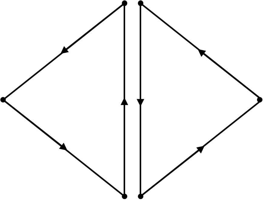
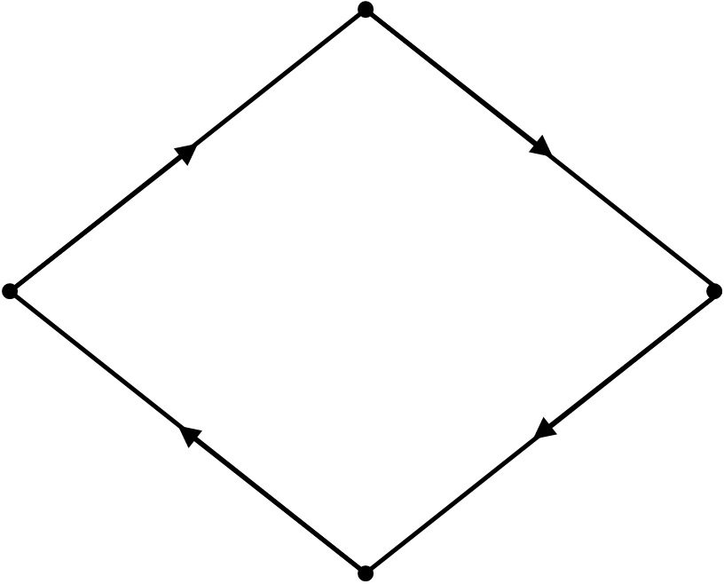
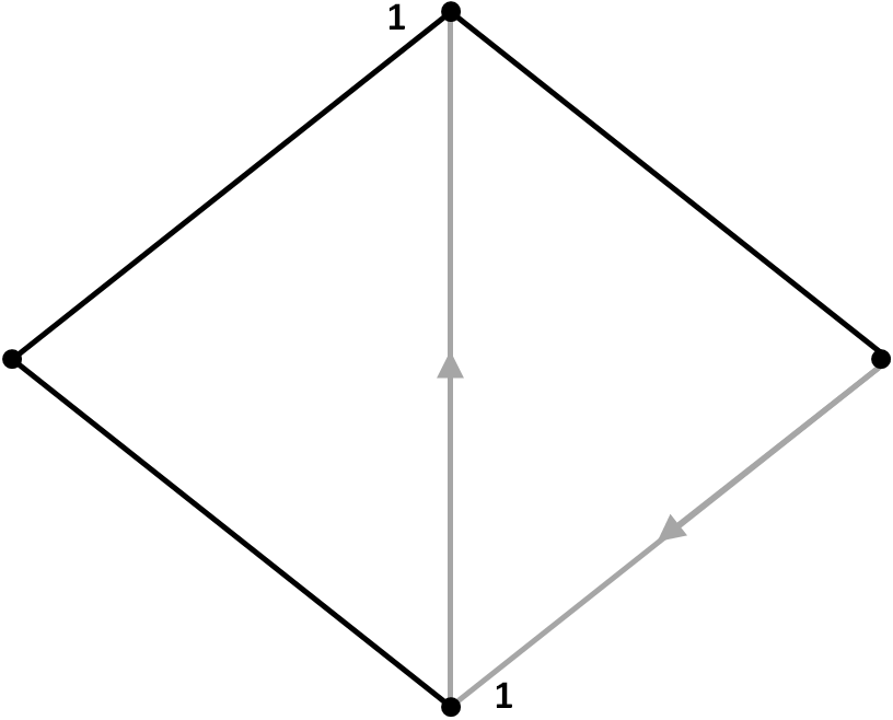
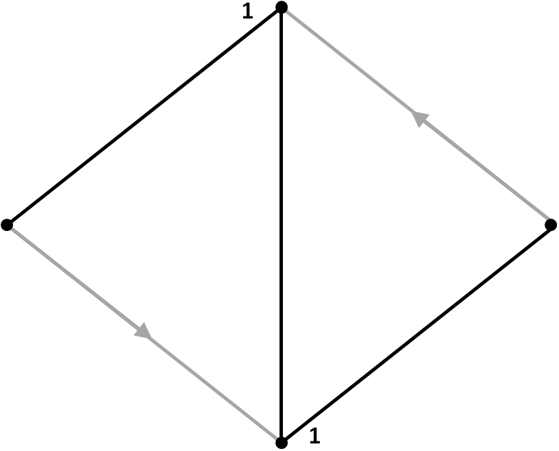
Figure 5 shows that not all cycle orientation configurations yield bijective cycle orientation maps, so the acyclic condition (1) is a non-trivial sufficient condition for a cycle orientation map to be bijective.

We mention two classes of objects that are indexed by the full-dimensional cones of the geometric bijection fan (equivalently, by geometric cycle orientation configurations), which might be of independent interests.

In particular, each full-dimensional cone of the geometric bijection fan induces a nice system of representatives for the cycle reversal system of $G$.

In [4], [11], the authors considered the notion of cycle minimal orientations: given an ordering $e_{1}<\ldots<e_{m}$ of the edges of $G$, together with a reference orientation, we say an orientation ${\mathcal{O}}$ is cycle minimal if every directed cycle is oriented according to the reference orientation of its minimum edge. Consider the cycle orientation configuration $\mathfrak{C}_{<}$ that orients each cycle according to its minimum edge. $\mathfrak{C}_{<}$ can be proven to be geometric (cf. Theorem 16 below), hence the notion of $\mathfrak{C}$-compatibility generalizes the notion of cycle minimality. The significance of such an observation is that the purely combinatorial notion of cycle minimal orientations has a natural generalization in terms of polyhedral geometry (an idea first briefly introduced in [25]), this suggests the possibility of generalizing other classical notions in combinatorics related to (edge) orderings to our setup.

The second class of objects we mention is the set of monomial initial ideals of the Lawrence ideal ${\mathcal{T}}_{G}$ associated to the cycle lattice $H_{1}(G,\mathbb{Z})$ of $G$. This ideal is also the ideal of the classical quasisymmetry model in statistics [29]. Formally, ${\mathcal{T}}_{G}\subset K[x_{1},\ldots,x_{m},y_{1},\ldots,y_{m}]$ is generated by binomials $\phi({\bf v})-\phi(-{\bf v})$ for ${\bf v}\in H_{1}(G,\mathbb{Z})$, where $\phi(a_{1}{\bf e}_{1}+\ldots+a_{m}{\bf e}_{m})=\prod_{a_{i}>0}x_{i}^{a_{i}}\prod_{a_{i}<0}y_{i}^{-a_{i}}$.

Geometrically, this is to say that the geometric bijection fan is the quotient of the Gröbner fan of ${\mathcal{T}}_{G}$ modulo a $(2m-g)$-dimensional lineality space.

By finding vectors that satisfy some stronger “genericity” conditions, we have a surprisingly simple family of geometric cycle orientation configurations/geometric bijections. But to the best of our knowledge, even such special cases are new in the literature.

We call the geometric bijections arising from edge orderings as in Theorem 16 as edge ordering maps/bijections. As explained in the proof of Proposition 11, each edge ordering map corresponds to the cone in the geometric bijection fan containing the vector $\sum_{i=1}^{m}\frac{1}{2^{i}}\pi(e_{i})$ in its interior.

References

- [1] Y. An, M. Baker, G. Kuperberg and F. Shokrieh. Canonical Representatives for Divisor Classes on Tropical Curves and the Matrix-Tree Theorem. Forum of Mathematics, Sigma 2, e24, 2014.
- [2] R. Bacher, P. de la Harpe and T. Nagnibeda. The Lattice of Integral Flows and the Lattice of Integral Cuts on a Finite Graph. Bulletin de la Société Mathématique de France 125(2), 167–198, 1997.
- [3] S. Backman. Riemann-Roch Theory for Graph Orientations. Advances in Mathematics 309, 655–691, 2017.
- [4] S. Backman. Partial Graph Orientations and the Tutte Polynomial. To appear in Advances in Applied Mathematics: Special issue on the Tutte polynomial. Available at http://arxiv.org/abs/1408.3962, 2014.
- [5] M. Baker and X. Faber. Metric Properties of the Tropical Abel-Jacobi Map. Journal of Algebraic Combinatorics 33(3), 349–381, 2011.
- [6] M. Baker and D. Jensen. Degeneration of Linear Series From the Tropical Point of View and Applications. In Nonarchimedean and Tropical Geometry, eds. M. Baker and S. Payne, Simons Symposia, Springer–Verlag, 365–433, 2016.
- [7] M. Baker and S. Norine. Riemann-Roch and Abel-Jacobi Theory on a Finite Graph. Advances in Mathematics 215(2), 766–788, 2007.
- [8] M. Baker and F. Shokrieh. Chip Firing Games, Potential Theory on Graphs, and Spanning Trees. Journal of Combinatorial Theory Series A 120(1), 164–182, 2013.
- [9] M. Baker and Y. Wang. The Bernardi Process and Torsor Structures on Spanning Trees. To appear in International Mathematics Research Notices. Available at http://arxiv.org/abs/1406.5084, 2014.
- [10] O. Bernardi. A Characterization of the Tutte Polynomial via Combinatorial Embedding. Annals of Combinatorics 12(2), 139–153, 2008.
- [11] O. Bernardi. Tutte Polynomial, Subgraphs, Orientations and Sandpile Model: New Connections via Embeddings. The Electronic Journal of Combinatorics 15(1), R109, 2008.
- [12] N. Biggs. Algebraic Potential Theory on Graphs. Bulletin London Mathematical Society 29(6), 641–682, 1997.
- [13] A. Björner, M. Las Vergnas, B. Sturmfels, N. White and G. Ziegler. Oriented Matroids, Second Edition. Encyclopedia of Mathematics and Its Applications 46, Cambridge University Press, Cambridge, 1999.
- [14] K. C. Border. Alternative Linear Inequalities. http://people.hss.caltech.edu/~kcb/Notes/Alternative.pdf, 2013.
- [15] M. Chan, T. Church and J. A. Grochow Rotor-routing and Spanning Trees on Planar Graphs. International Mathematics Research Notices 11, 3225–3244, 2015.
- [16] M. Chan, D. Glass, M. Macauley, D. Perkinson, C. Werner and Q. Yang. Sandpiles, Spanning Trees, and Plane Duality. SIAM Journal on Discrete Mathematics 29(1), 461–471, 2015.
- [17] D. Dhar and S. N. Majumdar. Equivalence between the Abelian Sandpile Model and the Limit of the Potts Model. Physica A 185, 129–145, 1992.
- [18] R. Diestel. Graph Theory, Third Edition. Graduate Texts in Mathematics 173, Springer, Berlin, 2006.
- [19] J. Ellenberg. “What is the Sandpile Torsor?”. Math Overflow, http://mathoverflow.net/questions/83552/, 2011.
- [20] S. Felsner. Lattice Structures from Planar Graphs. Journal of Combinatorics 11(1), R15, 2004.
- [21] A. Gathmann and M. Kerber. A Riemann-Roch Theorem in Tropical Geometry. Mathematische Zeitschrift 259(1), 217–230, 2008.
- [22] E. Gioan. Enumerating Degree Sequences in Digraphs and a Cycle-cocycle Reversing System. European Journal of Combinatorics 28(4), 1351–1366, 2007.
- [23] E. Gioan. Circuit-cocircuit Reversing Systems in Regular Matroids. Annals of Combinatorics 12(2), 171–182, 2008.
- [24] N. Goyal, L. Rademacher and S. Vempala. Expanders via Random Spanning Trees. Proceedings of SODA’09, 576–585, 2009.
- [25] C. Greene and T. Zaslavsky. On the Interpretation of Whitney Numbers through Arrangements of Hyperplanes, Zonotopes, Non-radon Partitions, and Orientations of Graphs. Transactions of the American Mathematical Society 280(1), 97–126, 1983.
- [26] J. Gross and T. Tucker. Topological Graph Theory. Wiley, New York, 1987.
- [27] A. Holroyd, L. Levine, K. Mészáros, Y. Peres, J. Propp and D. Wilson. Chip-firing and Rotor-routing on Directed Graphs. In In and Out of Equilibrium 2, eds. V. Sidoravicius and M. E. Vares, Progress in Probability 60, Birkhäuser, 331–364, 2008.
- [28] Scribed by S. Hopkins. Problems from the AIM Chip-Firing Workshop. http://web.mit.edu/~shopkins/docs/aim_chip-firing_problems.pdf, 2013.
- [29] M. Kateri, F. Mohammadi and B. Sturmfels. A Family of Quasisymmetry Models. Journal of Algebraic Statistics 6(1), 1–16, 2015.
- [30] L. Levine and J. Propp. “What is … a Sandpile?”. Notices of the AMS 57(8), 976–979, 2010.
- [31] A. Madry. Navigating Central Path with Electrical Flows: From Flows to Matchings, and Back. Proceedings of the Annual IEEE Symposium on Foundations of Computer Science, 253–262, 2013.
- [32] G. Mikhalkin and I. Zharkov. Tropical Curves, their Jacobians and Theta Functions. In Curves and Abelian Varieties, volume 465 of Contemporary Mathematics, 203–230. AMS, Providence, RI, 2008.
- [33] F. Mohammadi and F. Shokrieh. Divisors on Graphs, Binomial and Monomial Ideals, and Cellular Resolutions. Mathematische Zeitschrift 283(1), 59–102, 2016.
- [34] R. Stanley. A Zonotope Associated with Graphical Degree Sequences. In Applied Geometry and Discrete Mathematics, volume 4 of DIMACS: Series in Discrete Mathematics and Theoretical Computer Science, 555–570. AMS, Providence, RI, 1991.
- [35] B. Sturmfels. Grobner Bases and Convex Polytopes. University Lecture Series 8. AMS, Providence, RI, 1996.
School of Mathematics, Georgia Institute of Technology
Atlanta, Georgia 30332-0160, USA
Email address: cyuen7@math.gatech.edu