Inequality measures in kinetic exchange models of wealth distributions

Asim Ghosh Email: asim.ghosh@saha.ac.in Affiliation: Condensed Matter Physics Division, Saha Institute of Nuclear Physics, 1/AF Bidhannagar, Kolkata 700064, India. Affiliation: Department of Computer Science, Aalto University School of Science, P.O. Box 15400, FI-00076 AALTO, Finland Arnab Chatterjee Email: arnabchat@gmail.com Affiliation: Condensed Matter Physics Division, Saha Institute of Nuclear Physics, 1/AF Bidhannagar, Kolkata 700064, India. Jun-ichi Inoue Thanks: deceased Affiliation: Graduate School of Information Science & Technology, Hokkaido University, N14-W9, Kita-ku, Sapporo 060-0814, Japan. Bikas K. Chakrabarti Email: bikask.chakrabarti@saha.ac.in Affiliation: Condensed Matter Physics Division, Saha Institute of Nuclear Physics, 1/AF Bidhannagar, Kolkata 700064, India. Affiliation: Economic Research Unit, Indian Statistical Institute, 203 B. T. Road, Kolkata 700108, India.

Abstract

In this paper, we study the inequality indices for some models of wealth exchange. We calculated Gini index and newly introduced $k$ -index and compare the results with reported empirical data available for different countries. We have found lower and upper bounds for the indices and discuss the efficiencies of the models. Some exact analytical calculations are given for a few cases. We also exactly compute the quantities for Gamma and double Gamma distributions.

Keywords:

kinetic models of wealth distribution, inequality, Gini index

I Introduction

Socio-economic inequality [1, 2, 3, 4] is manifested in the existence of unequal rewards and opportunities for social positions or statuses in a society. Structured, recurrent patterns of unequal distributions of goods, wealth, opportunities, rewards and punishments are mainly measured in terms of inequality of conditions, and inequality of opportunities. The former refers to the unequal distribution of income, wealth and material goods, while the latter refers to the unequal distribution of ‘life chances’ of individuals. This is somehow reflected in measures such as level of education, health status, and treatment by the criminal justice system. Socio-economic inequality often results in crisis, political unrest and instability, conflict, war, criminal activity and finally affects economic growth [5]. Initially, economic inequalities were studied in the context of income and wealth [6, 7, 8], but the notions and observations have led to widespread research, see e.g. Ref. [9, 10] for various socio-economic inequalities. The study of inequality in society [11, 12, 13] is a topic of global focus and utmost current interest, bringing together researchers from various disciplines.

By the end of the 19th century, Pareto [14] made extensive studies and found that wealth distribution in Europe follows a power law for the rich, commonly known to be the Pareto law. Subsequent studies have revealed that the distributions of income and wealth possess some globally robust features (see, e.g., [7]): the bulk of both the income and wealth distributions seem to reasonably fit both the log-normal and the Gamma distributions. Economists have a preference for the log-normal distribution [15, 16], while statisticians [17] and physicists [18, 19, 6] root for the Gamma distribution for the probability density or Gibbs/exponential distribution for the corresponding cumulative distribution. The high end of the distribution, known as the ‘tail’, is well described by a power law as observed by Pareto. Formally, the probability distribution of wealth is given by

P(m)\sim\left\{\begin{array}[]{lc}F(m)&\textrm{for}\ m<m_{c},\\ \frac{\alpha m_{c}^{\nu}}{m^{1+\nu}}&\textrm{for}\ m\geq m_{c},\end{array}\right.

(1)

where $\alpha$ is a constant and $\nu$ is called the Pareto exponent, ranging between 1 and 3 [7] (See Ref. [20] for a historical account of Pareto’s data and some recent sources). $F(m)$ is some function which could be exponential, Gamma or lognormal. The crossover point $m_{c}$ is extracted from the numerical fittings.

One of the key class of models uses the kinetic theory of gases [21], where the gas molecules colliding and exchanging energy was mapped to agents meeting to exchange wealth, following certain rules [19]. In these models, a pair of agents agree to trade, each save a fraction $\lambda$ of their instantaneous money/wealth and exchanges a random fraction of the rest at each trading step. The distribution of wealth in the steady state, $P(m)$ matches well with the empirical data. When the saving fraction $\lambda$ is fixed, i.e., in case of homogeneous agents (CC model hereafter) [22], $P(m)$ are very well approximated to Gamma distributions [23]. It is important to note that, in reality, the richest follow a different dynamic where heterogeneity plays the key role. To obtain the power law distribution of wealth for the richest, one needs simply to consider each agent as different in terms of the fraction of wealth he/she saves in each trading [24], which is very natural to assume, because it is quite likely that agents in a market think differently from one another. With this very little modification, one can explain the whole range of wealth distribution [19]. When $\lambda$ is distributed uniformly in $[0,1)$ and quenched, (CCM model hereafter), i.e., for heterogeneous agents, one obtains a Pareto law for the probability density of wealth $P(m)\sim m^{-\nu}$ with exponent $\nu=2$ [24, 19]. Several variants of these models, find possible applications in a variety of trading processes [7, 25].

Socio-economic inequalities are quantified in various ways. The most popular measures are absolute, in terms of indices, e.g., Gini [16], Theil [26], Pietra [27] and the recently introduced $k$ index [28]. The alternative approach is a relative measure, in terms of probability distributions of various quantities, but the most of the above mentioned indices can be computed from the distributions. Most quantities often display broad distributions, usually lognormals, power-laws or their combinations. For example, the distribution of income is usually an exponential followed by a power law [29] (see Ref.[7] for other examples).

To compute the Gini index, one has to consider the Lorenz curve [30], that represents the cumulative proportion $X$ of ordered individuals (from lowest to highest) in terms of the cumulative proportion of their sizes $Y$ (See Fig. 1a). $X$ can represent income or wealth of individuals. The Gini index ( $g$ ) is defined as the ratio between the area enclosed between the Lorenz curve and the equality line, to that below the equality line. If the area between (i) the equality line and the Lorenz curve is $A$ , and (ii) that below the Lorenz curve as $B$ , the Gini index is given by $g=A/(A+B)$ . The recently introduced ‘ $k$ index’ [28] is defined as the fraction $k$ such that $(1-k)$ fraction of individuals possess $k$ fraction of income or wealth (See Fig. 1a) [31].

In this paper, we investigate the inequality in wealth in some models of wealth distribution which are inspired by kinetic theory of gases. We mainly discuss the results for two well studied models (CC and CCM) and a new model for bimodal distribution of wealth. We numerically compute the inequality indices, Gini index and $k$ -index to quantify the inequalities. Gini index $g$ , the most popular and widely used measure for inequality in case of income and wealth distribution, can take value from $0$ to $1$ . The value $g=0$ refers to complete equality and $g=1$ represents completely inequality. The meaning of $k$ -index, say, for a wealth distribution, is the following: $k$ fraction of the top wealthiest people possess $1-k$ fraction of total wealth. We found that in both CC and CCM models there are some upper and lower limits of the indices. For CC model, $g$ varies between $0$ and $0.5$ , and $k$ from $0.5$ to $0.68$ . Similarly, for CCM model, $g$ varies between $0.4$ to $0.85$ . Therefore, both models independently do not cover the possible theoretical range of values of $g$ and $k$ . We find that the range of $g$ as found from empirical data ( $0.2-0.7$ ) (see Fig. 1, using World Bank data [32]) can be well covered by CCM model. We also considered a model where two groups of agents have fixed but different saving propensities. Depending on the combinations, the resulting probability distribution of wealth is found to be unimodal or bimodal. The phase boundaries, depending on the ratio of the two groups and the combination of values of their saving propensities are also computed numerically. The bimodal distribution seems to fit well to a combination of two gamma distributions (double -Gamma distribution). Gini index and $k$ index are calculated for this model for different combination of parameters. Next, we considered gamma and double-Gamma distribution and computed certain quantities like Lorenz curve and Gini indices.

Refer to caption — Figure 1: (a) Gini and $k$ -index schematic: the solid red line is the Lorez curve, the cumulative proportion $X$ of ordered individuals (from lowest to highest) in terms of the cumulative proportion of their sizes $Y$ . Gini index is given by the ratio $g=A/(A+B)$ . The $k$ -index is computed from the intersection ( $k,1-k$ ) of the reverse diagonal with the Lorenz curve. (b) Gini index from World Bank data [32] for several countries over years.

II Models and numerical simulation results

Kinetic exchange models of wealth distributions [19] serve as simple paradigmatic models for exchange of wealth in an economy. The main idea is that agents possess wealth $m_{i}$ which is redistributed upon trading with others. The ‘economy’ is assumed to be a ‘closed’ one, in the sense that neither the number of agents change nor does that total amount of wealth in the system, and the economic activity is limited to exchange of wealth according to certain rules. The basic model in the framework is just the random sharing of wealth, motivated by random exchange of energy between gas molecules, as in the framework of kinetic theory of gases [6]. The basic money exchange model [21] imitates the kinetic exchange in an ideal gas, but subsequently developed models incorporate the notion of ‘savings’. In the following, we discuss these models, and also compute the inequality measures like Gini and $k$ -index.

II.1 CC model

Savings come as a natural ingredient in a trading economy. In each trading step, a pair of agents exchange their wealth in the following way: they keep a fixed fraction $\lambda$ of their wealth to themselves and the rest $1-\lambda$ fraction is pooled up to be randomly split among the two [22]. In this model (CC model hereafter), agents are homogeneous – all of them save the same fraction of their instantaneous wealth at each trading step. Formally, the dynamics is defined by

	$\displaystyle m_{i}(t+1)$	$\displaystyle=\lambda m_{i}(t)+r(1-\lambda)\left(m_{i}(t)+m_{j}(t)\right)$		(2)
	$\displaystyle m_{j}(t+1)$	$\displaystyle=\lambda m_{j}(t)+(1-r)(1-\lambda)(m_{i}(t)+m_{j}(t)),$		(2)

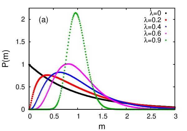
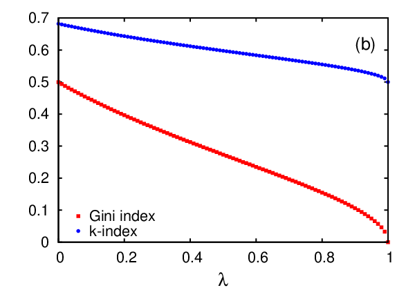
where $r$ is a random fraction in $[0,1]$ , drawn in each time (exchange) step. $m_{i}(t)$ and $m_{i}(t+1)$ are the wealth of the $i$ th agent at trading times $t$ and $(t+1)$ respectively. The ‘saving propensity’ $\lambda$ is a fixed fraction in $[0,1)$ . $\lambda=0$ corresponds to complete random exchange (DY model) while $\lambda=1$ gives no dynamics. For $\lambda=0$ , $P(m)=\exp(-m/\langle m\rangle)$ is exponential, for which Lorenz curve, Gini and $k$ index were derived [31]. However, for finite $\lambda$ , $P(m)=Cm^{\alpha}\exp(-m/T)$ , has a form of Gamma distribution [23], where $T=\frac{1}{1+\alpha}$ and $C=\frac{(\alpha+1)^{(\alpha+1)}}{\Gamma(\alpha+1)}$ . The exponent $\alpha$ is related to the parameter $\lambda$ as $\alpha=\frac{3\lambda}{1-\lambda}$ . We plot $P(m)$ vs. $m$ for different values of $\lambda$ in Fig 2a. For these simulations (and for each case discussed in the paper), the average wealth $\langle m\rangle$ is set to unity. We measured inequality in the distributions in terms of Gini and $k$ index and plotted in Fig. 2b for different values of $\lambda$ .

II.2 CCM model

In this model [24, 19] (CCM model hereafter), agents are assumed to be heterogeneous, the saving fraction $\lambda$ for each agent is different, drawn from a given distribution

\Pi(\lambda)=(1+\delta)(1-\lambda)^{\delta},{\rm with}-1<\delta<\infty,

(3)

where $\lambda$ is a fraction in the interval $[0,1-\epsilon]$ , where $\epsilon$ is arbitrarily small and positive. The dynamics of exchange follows

	$\displaystyle m_{i}(t+1)$	$\displaystyle=\lambda_{i}m_{i}(t)+r((1-\lambda_{i})m_{i}(t)+(1-\lambda_{j})m_{j}(t))$		(4)
	$\displaystyle m_{j}(t+1)$	$\displaystyle=\lambda_{j}m_{j}(t)+(1-r)((1-\lambda_{i})(m_{i}(t)+(1-\lambda_{j})m_{j}(t)),$		(4)

where $r$ is a random fraction in $[0,1]$ , drawn in each time (exchange) step. $\lambda_{i}$ is the saving fraction of agent $i$ whose wealth is $m_{i}(t)$ at trading step $t$ . $\lambda_{i}$ are quenched and drawn randomly from $\Pi(\lambda)$ (Eq. 3). The asymptotic form of the steady state distribution of wealth is given by [19]

\displaystyle P(m)\sim m^{-(2+\delta)}.

(5)

We compute $P(m)$ vs. $m$ for different values of $\delta$ . In the simulations, we allow values of $\lambda$ until a certain fixed upper cutoff ( $0.999$ for our case; i.e., $\epsilon=0.001$ ), because the population of agents with $\lambda$ close to $1$ is already high, and we have to restrict any agent assuming a saving propensity very close to unity. As a result, there is no finite size effect in the calculated values.

In Fig. 3a we plot the distributions $P(m)$ for non-negative values of $\delta$ . We find that the probability distribution $P(m)$ follows Eq. 5 for most of the range of $m$ , until an exponential cut-off, which is a result of the truncation of $\Pi(\lambda)$ close to $1$ . In Fig. 3b we plot the same for negative values of $\delta$ . The probability distribution $P(m)$ again follows Eq. 5 for most of the range of $m$ . However, it is quite interesting to note that for $\delta\lesssim-0.5$ , $P(m)$ shows a second peak at a large value of $m$ , say $m_{*}$ . This $m_{*}$ moves towards $\langle m\rangle=1$ as $\delta\to-1$ . This is quite easy to explain theoretically: as $\delta\to-1$ , $\Pi(\lambda)$ is peaked near $\lambda\to 1$ , essentially more and more fraction of agents have very high saving propensities, a situation similar to $\lambda\to 1$ in CC model. We recall that this situation will tend to produce $P(m)$ peaked at average money per agent ( $\langle m\rangle=1$ ), which is equivalent to more “equality”. $P(m)=\Delta(m-\langle m\rangle)$ with $\langle m\rangle=1$ for $\lambda=1$ in CC model; here $\Delta(\cdot)$ is the Dirac delta function. Then Gini index $g=0$ and $k=0.5$ . In comparison, $\lambda$ are distributed in CCM model and making $\delta\to-1$ makes $\Pi(\lambda)$ further peaked near $\lambda=1$ , more agents have ‘similar’ values of saving, close to unity and produce the second peak close to $m=\langle m\rangle=1$ . The peak moves towards $\langle m\rangle$ as $\delta\to-1$ . Additionally, Gini index $g\to 0$ . It may be noted that, because of this modification over the power law (Eq. 5) in the distribution function $P(m)$ , the standard relationship between Gini index and the Pareto exponent (see e.g., Ref. [7]) is not valid here.

We measured inequality in the distributions in terms of Gini and $k$ -indices and plotted in Fig. 3(c) for different values of $\delta$ . Inequality seems to be maximum around $\delta\approx-0.5$

II.3 Model for bimodal distribution and phase diagram

Bimodal distributions in wealth distributions are not uncommon [20], and is also observed in firm sizes [33]. In the following we propose a very simple modification in the kinetic exchange model framework, to produce bimodal distribution of wealth.

Let us now consider two groups of $N_{1}$ and $N_{2}$ agents, with saving propensities $\lambda_{1}$ and $\lambda_{2}$ respectively. Let $p=N_{1}/(N_{1}+N_{2})$ . Agents’ saving propensities remain unchanged over time, and they exchange money using the same rule as CC model (Eq. 2). For example, let us consider the case $p=0.5$ i.e., $N_{1}=N_{2}$ . Let $\lambda_{1}=0.2$ and $\lambda_{2}=0.8$ . After exchanging their money, the steady state distribution is shown in Fig. 4. The distribution clearly shows bimodal distribution. We fit the distribution with a combination of two Gamma distributions $a_{1}m^{\alpha_{1}}e^{-\beta_{1}m}+a_{2}m^{\alpha_{2}}e^{-\beta_{2}m}$ with parameter values $\alpha_{1}=0.98$ , $\alpha_{2}=10.57$ , $\beta_{1}=4.82$ and $\beta_{2}=7.23$ as shown in the Fig 4a. We found that all combinations of ( $\lambda_{1},\lambda_{2}$ ) do not give the bimodal distributions. The combination of values giving bimodal distribution are shown in the phase diagram. The boundary region is roughly estimated for various values of $p$ ( $=0.1,0.2,0.3,0.4,0.5$ ) and shown in Fig. 4b. We also computed Gini index and $k$ -index for different combination of ( $\lambda_{1},\lambda_{2}$ ) for various values of $p$ (Fig. 5).

III Gamma distribution and its inequality statistics

For the CC model, the steady state wealth distribution closely fits gamma distributions [23]. Let us compute the inequality measures considering such a distribution. For the Gamma distribution:

P(m)\propto m^{\alpha}{\rm e}^{-\beta m},\,\,\,\beta\equiv 1/T

(6)

we evaluate the inequality statistics. The cumulative distribution is given as

x(r)=\int_{0}^{r}m^{\alpha}{\rm e}^{-\beta m}dm=\frac{\gamma(\alpha+1,\beta r)}{\beta^{1+\alpha}}

(7)

where $\gamma(a,x)$ is an incomplete gamma function defined by

\gamma(a,x)=\int_{0}^{x}t^{a-1}{\rm e}^{-t}dt.

(8)

Hence, we have the normalization constant of the distribution (6) as

x(\infty)=\frac{\Gamma(\alpha+1)}{\beta^{1+\alpha}}

(9)

where we define the Gamma function by

\Gamma(a)=\int_{0}^{\infty}t^{a-1}{\rm e}^{-t}dt=\gamma(a,\infty).

(10)

Thus, we have

X(r)\equiv\frac{x(r)}{x(\infty)}=\frac{\gamma(\alpha+1,\beta r)}{\Gamma(\alpha+1)}.

(11)

Similarly, we have

y(r)=\frac{1}{\beta^{2+\alpha}}\int_{0}^{\beta r}m^{\alpha+1}{\rm e}^{-m}dm=\frac{\gamma(\alpha+2,\beta r)}{\beta^{2+\alpha}}

(12)

and

y(\infty)=\frac{\Gamma(\alpha+2)}{\beta^{2+\alpha}}

(13)

Hence,

Y(r)\equiv\frac{y(r)}{y(\infty)}=\frac{\gamma(\alpha+2,\beta r)}{\Gamma(\alpha+2)}.

(14)

Therefore, the Lorentz curve is given by (11) and (14). In Fig. 6a, we plot the Lorentz curve for several values of $\alpha$ . We also checked numerically that the curve is independent of the parameter $\beta$ . Next, to calculate Gini index, we check if the following relation is satisfied:

\gamma(a+1,x)=a\gamma(a,x)-x^{a}{\rm e}^{-x}

(15)

Applying it to our case, we immediately obtain

\gamma(\alpha+2,\beta r)=(\alpha+1)\gamma(\alpha+1,\beta r)-(\beta r)^{\alpha+1}{\rm e}^{-\beta r}.

(16)

This reads

\Gamma(\alpha+2)Y=(\alpha+1)\Gamma(\alpha+1)X-(\beta r)^{\alpha+1}{\rm e}^{-\beta r}.

(17)

If we notice $\Gamma(\alpha+2)=(\alpha+1)\Gamma(\alpha+1)$ , we obtain

X-Y=\frac{(\beta r)^{\alpha+1}{\rm e}^{-\beta r}}{\Gamma(\alpha+2)}.

(18)

Accompanying the derivative

\frac{dX}{dr}=\beta\frac{(\beta r)^{\alpha}{\rm e}^{-\beta r}}{\Gamma(\alpha+1)}

(19)

with $X-Y$ , we get the Gini index $g$ as

$\displaystyle g$	$\displaystyle=$	$\displaystyle 2\int_{0}^{1}(X-Y)dX$	(20)
	$\displaystyle=$	$\displaystyle 2\beta\int_{0}^{\infty}\frac{(\beta r)^{\alpha+1}{\rm e}^{-\beta r}}{\Gamma(\alpha+2)}\cdot\frac{(\beta r)^{\alpha}{\rm e}^{-\beta r}}{\Gamma(\alpha+1)}dr$
	$\displaystyle=$	$\displaystyle\frac{2\beta}{\Gamma(\alpha+2)\Gamma(\alpha+1)}\int_{0}^{\infty}(\beta r)^{2\alpha+1}{\rm e}^{-2\beta r}dr=\frac{\Gamma(2(\alpha+1))}{2^{2\alpha+1}\Gamma(\alpha+1)\Gamma(\alpha+2)}.$

which is independent of $\beta$ and we recover the exponential case by setting $\alpha=0$ as

g_{0}=\frac{\Gamma(2)}{2\Gamma(1)\Gamma(2)}=\frac{1}{2}.

(21)

Note $\Gamma(1)=1$ . The cases of $\alpha=1,2$ are given by

	$\displaystyle g_{1}$	$\displaystyle=$	$\displaystyle\frac{\Gamma(4)}{2^{3}\Gamma(2)\Gamma(3)}=\frac{3}{8}$		(22)
	$\displaystyle g_{2}$	$\displaystyle=$	$\displaystyle\frac{\gamma(6)}{2^{5}\Gamma(3)\Gamma(4)}=\frac{5}{16}$		(23)

where we used $\Gamma(\alpha+1)=\alpha\Gamma(\alpha)$ recursively. In Fig. 6, we plot the $g$ as a function of $\alpha$ , and values of $g$ corresponding to $\alpha=1,2$ are also indicated.

IV Mixture of Gamma distributions: Unimodal and bimodal distribution

We next consider the mixture of Gamma distribution as

P(x)=(1-f)x^{\kappa_{1}-1}\frac{{\rm e}^{-x/\theta_{1}}}{\Gamma(\kappa_{1})\theta_{1}^{\kappa_{1}}}+fx^{\kappa_{2}-1}\frac{{\rm e}^{-x/\theta_{2}}}{\Gamma(\kappa_{2})\theta_{2}^{\kappa_{2}}}

(24)

Obviously, for $f=0$ , the unimodal Gamma distribution takes its maximum at $x=\theta_{1}(\kappa_{1}-1)$ . However, for $a\neq 1$ , the peaks are located at the $x$ as solutions of

\frac{1-f}{\Gamma(\kappa_{1})\theta_{1}^{\kappa_{1}+1}}\left(\theta_{1}(\kappa_{1}-1)-x\right)x^{\kappa_{1}-1}{\rm e}^{-x/\theta_{1}}+\frac{f}{\Gamma(\kappa_{2})\theta_{2}^{\kappa_{2}+1}}\left(\theta_{2}(\kappa_{2}-1)-x\right)x^{\kappa_{2}-1}{\rm e}^{-x/\theta_{2}}=0

(25)

Hence, the locations of the peaks are dependent on the choice of parameters $\theta_{1},\theta_{2},\kappa_{1},\kappa_{2},f$ . For the Lorentz curve, we obtain

	$\displaystyle X(r)$	$\displaystyle=$	$\displaystyle\frac{(1-f)}{\Gamma(\kappa_{1})}\gamma(\kappa_{1},r/\theta_{1})+\frac{f}{\Gamma(\kappa_{2})}\gamma(\kappa_{2},r/\theta_{2})$		(26)
	$\displaystyle Y(r)$	$\displaystyle=$	$\displaystyle\frac{\frac{(1-f)}{\Gamma(\kappa_{1})}\theta_{1}\gamma(\kappa_{1}+1,r/\theta_{1})+\frac{f}{\Gamma(\kappa_{2})}\theta_{2}\gamma(\kappa_{2}+1,r/\theta_{2})}{Y(\infty)}$		(27)

where we defined

Y(\infty)=(1-f)\theta_{1}\left\{\frac{\Gamma(\kappa_{1}+1)}{\Gamma(\kappa_{1})}\right\}+f\theta_{2}\left\{\frac{\Gamma(\kappa_{2}+1)}{\Gamma(\kappa_{2})}\right\}.

(28)

In Fig 7b, we plot the Lorentz curve for several choices of the parameters. For the above Lorentz curve, the Gini index $g(f,\kappa_{1},\kappa_{2},\theta_{1},\theta_{2})$ is calculated as

$\displaystyle g$	$\displaystyle=$	$\displaystyle\left\{\frac{1-f}{\Gamma(\kappa_{1})}\right\}^{2}\frac{1}{\theta_{1}^{\kappa_{1}}}\int_{0}^{\infty}dr\,r^{\kappa_{1}-1}{\rm e}^{-r/\theta_{1}}\{\gamma(\kappa_{1},r/\theta_{1})-\frac{\theta_{1}}{Y(\infty)}\gamma(\kappa_{1}+1,r/\theta_{1})\}$	(29)
	$\displaystyle+$	$\displaystyle\frac{f(1-f)}{\theta_{1}^{\kappa_{1}}\Gamma(\kappa_{1})\Gamma(\kappa_{2})}\int_{0}^{\infty}dr\,r^{\kappa_{1}-1}{\rm e}^{-r/\theta_{1}}\{\gamma(\kappa_{2},r/\theta_{2})-\frac{\theta_{2}}{Y(\infty)}\gamma(\kappa_{2}+1,r/\theta_{2})\}$
	$\displaystyle+$	$\displaystyle\frac{f(1-f)}{\theta_{2}^{\kappa_{2}}\Gamma(\kappa_{1})\Gamma(\kappa_{2})}\int_{0}^{\infty}dr\,r^{\kappa_{2}-1}{\rm e}^{-r/\theta_{2}}\{\gamma(\kappa_{1},r/\theta_{1})-\frac{\theta_{1}}{Y(\infty)}\gamma(\kappa_{1}+1,r/\theta_{1})\}$
	$\displaystyle+$	$\displaystyle\left\{\frac{f}{\Gamma(\kappa_{2})}\right\}^{2}\frac{1}{\theta_{2}^{\kappa_{2}}}\int_{0}^{\infty}dr\,r^{\kappa_{2}-1}{\rm e}^{-r/\theta_{2}}\{\gamma(\kappa_{2},r/\theta_{2})-\frac{\theta_{2}}{Y(\infty)}\gamma(\kappa_{2}+1,r/\theta_{2})\}.$

Knowing the parameters $f,\kappa_{1},\kappa_{2},\theta_{1},\theta_{2}$ , one can compute $g$ numerically from the above expression.

V Discussion

Empirical data [32] shows that Gini index varies mostly in $0.2-0.7$ (see Fig. 1b). The CC model gives Gini index in the range $0-0.5$ . The inequality decreases monotonically with increasing saving propensity $\lambda$ . $g=0.5$ for $\lambda=0$ , the wealth distribution $P(m)$ is a perfect exponential distribution, giving the maximum value of inequality for this model. On the other extreme, when $\lambda\to 1$ , $P(m)$ approaches a Dirac $\delta$ -function $\Delta(m-\langle m\rangle)$ , for which $g\to 0$ (Fig. 2). Hence this model does not reproduce most of the range of real Gini indices. In reality, Gini index rarely go below $0.3$ , but often goes beyond $0.5$ .

In CCM model, however, the range of the Gini index is quite wide, and in fact, overlaps with almost the entire range of empirically observed Gini index values. In fact, in the asymptotic limit of Eq. 5 for practically infinite value of $\delta$ , $P(m)$ should approach an uniform distribution in $[0,1]$ , which will yield a value of Gini index equal to $1/3$ . In Fig. 3b, we observe that for large values of $\delta$ , there is a tendency to saturate to a value close to $0.4$ , which we anticipate, might as well approach $1/3$ for $\delta\to\infty$ .

In some empirical analysis, the bulk of the wealth distribution resembles Gamma distribution. We analytically computed the Lorenz curve and the Gini index for Gamma distributions. There are even some instances where the wealth distribution are found to be double peaked [20]. We propose a variation of the kinetic exchange models to model this, and a combination of Gamma distributions to fit the resulting distribution. The steady state distribution is unimodal or bimodal depending on the combination of values of the saving propensities and the relative fraction of agents of the two groups. The phase boundaries for specific cases have been computed using numerical simulations. We also show that it is possible to derive an exact expression for the Gini index, considering Gamma distribution as the best fit to the numerically computed steady state wealth distributions.

The critical studies of kinetic exchange models of wealth distributions seem to yield more and more interesting aspects, not only in terms of theoretical understanding of the models, but also when compared to empirical data. For instance, one of the recent studies explain city size statistics using the same framework [34]. There has not been only a very few studies [35] that discuss inequality measures in reference to models. Further research will be able to elucidate the usefulness of such a simple framework in understanding complex socio-economic phenomena.

Acknowledgements.

A.C. and B.K.C. acknowledge support from B.K.C.’s J. C. Bose Fellowship Research Grant.

References

[1] K. J. Arrow, S. Bowles, S. N. Durlauf, Meritocracy and economic inequality, Princeton Univ. Press, 2000.
[2] J. E. Stiglitz, The price of inequality: How today’s divided society endangers our future, WW Norton & Company, 2012.
[3] K. Neckerman, Social Inequality, Russell Sage Foundation, 2004.
[4] J. H. Goldthorpe, Analysing social inequality: a critique of two recent contributions from economics and epidemiology, Eur. Sociological Rev. 26 (6) (2010) 731–744.
[5] C. E. Hurst, Social Inequality: Forms, Causes, and Consequences, Allyn and Bacon, Boston, 1995.
[6] V. M. Yakovenko, J. Barkley Rosser Jr., Colloquium: Statistical mechanics of money, wealth and income, Rev. Mod. Phys. 81 (2009) 1703–1725.
[7] B. K. Chakrabarti, A. Chakraborti, S. R. Chakravarty, A. Chatterjee, Econophysics of income and wealth distributions, Cambridge Univ. Press, Cambridge, 2013.
[8] H. Aoyama, Y. Fujiwara, Y. Ikeda, Econophysics and companies: statistical life and death in complex business networks, Cambridge Univ. Press, Cambridge, 2010.
[9] A. Chatterjee, Socio-economic inequalities: a statistical physics perspective, in: Econophysics and Data Driven Modelling of Market Dynamics, Eds. F Abergel, H. Aoyama, B.K. Chakrabarti, A. Chakraborti, A. Ghosh,, New Economic Windows, Springer (2015), 2014.
[10] A. Chatterjee, A. Ghosh, J.-I. Inoue, B. K. Chakrabarti, Social inequality: from data to statistical physics modeling, J. Phys. Conf. Ser. 638 (2015) 012014.
[11] A. Cho, Physicists say it’s simple, Science 344 (6186) (2014) 828.
URL http://www.sciencemag.org/content/344/6186/828.short
[12] G. Chin, E. Culotta, What the numbers tell us, Science 344 (6186) (2014) 818–821.
URL http://www.sciencemag.org/content/344/6186/818.short
[13] Y. Xie, Undemocracy: Inequalities in science, Science 344 (6186) (2014) 809–810.
URL http://www.sciencemag.org/content/344/6186/809.short
[14] V. Pareto, Cours d’economie politique, Rouge, Lausanne, 1897.
[15] E. W. Montroll, M. F. Shlesinger, On 1/f noise and other distributions with long tails, Proc. Natl. Acad. Sci. 79 (1982) 3380–3383.
[16] C. Gini, Measurement of inequality of incomes, Econ. J. 31 (121) (1921) 124–126.
[17] R. Hogg, J. Mckean, A. Craig, Introduction to mathematical statistics, Pearson Education, Delhi, 2007.
[18] A. Chatterjee, S. Yarlagadda, B. K. Chakrabarti (Eds.), Econophysics of Wealth Distributions, New Economic Windows Series, Springer-Verlag, Milan, 2005.
[19] A. Chatterjee, B. K. Chakrabarti, Kinetic exchange models for income and wealth distributions, Eur. Phys. J. B 60 (2) (2007) 135–149.
[20] P. Richmond, S. Hutzler, R. Coelho, P. Repetowicz, A review of empirical studies and models of income distributions in society, in: B. K. Chakrabarti, A. Chakraborti, A. Chatterjee (Eds.), Econophysics and Sociophysics: Trends and Perspectives, Wiley-VCH, Weinheim, 2007, pp. 131–159.
[21] A. A. Drăgulescu, V. M. Yakovenko, Statistical mechanics of money, Eur. Phys. J. B 17 (2000) 723–729.
[22] A. Chakraborti, B. K. Chakrabarti, Statistical mechanics of money: how saving propensity affects its distribution, Eur. Phys. J. B 17 (2000) 167–170.
[23] M. Patriarca, A. Chakraborti, K. Kaski, Statistical model with a standard $\Gamma$ distribution, Phys. Rev. E 70 (1) (2004) 016104.
[24] A. Chatterjee, B. K. Chakrabarti, S. S. Manna, Pareto law in a kinetic model of market with random saving propensity, Physica A 335 (2004) 155–163.
[25] L. Pareschi, G. Toscani, Interacting Multiagent Systems: Kinetic Equations and Monte Carlo Methods, Oxford Univ. Press, Oxford, 2013.
[26] H. Theil, Economics and information theory, North-Holland Amsterdam, 1967.
[27] I. I. Eliazar, I. M. Sokolov, Measuring statistical heterogeneity: The pietra index, Physica A 389 (1) (2010) 117–125.
[28] A. Ghosh, N. Chattopadhyay, B. K. Chakrabarti, Inequality in societies, academic institutions and science journals: Gini and k-indices, Physica A 410 (14) (2014) 30–34.
[29] A. A. Drăgulescu, V. M. Yakovenko, Exponential and power-law probability distributions of wealth and income in the united kingdom and the united states, Physica A 299 (1) (2001) 213–221.
[30] M. O. Lorenz, Methods for measuring the concentration of wealth, Am. Stat. Assoc. 9 (1905) 209–219.
[31] J.-I. Inoue, A. Ghosh, A. Chatterjee, B. K. Chakrabarti, Measuring social inequality with quantitative methodology: analytical estimates and empirical data analysis by gini and $k$ indices, Physica A 429 (2015) 184–204.
[32] World Bank, All the Ginis Dataset, retrieved June, 2014, http://siteresources.worldbank.org/INTRES/Resources/469232-1107449512766/allgini s_2013.xls.
[33] A. S. Chakrabarti, Bimodality in the firm size distributions: a kinetic exchange model approach, Eur. Phys. J. B 86 (6) (2013) 1–6.
[34] A. Ghosh, A. Chatterjee, A. S. Chakrabarti, B. K. Chakrabarti, Zipf’s law in city size from a resource utilization model, Phys. Rev. E 90 (4) (2014) 042815.
[35] A. S. Chakrabarti, B. K. Chakrabarti, Inequality reversal: Effects of the savings propensity and correlated returns, Physica A 389 (17) (2010) 3572–3579.