Microscopic theory of the residual surface resistivity of Rashba electrons
Abstract
A microscopic expression of the residual electrical resistivity tensor is derived in linear response theory for Rashba electrons scattering at a magnetic impurity with cylindrical or non-cylindrical potential. The behavior of the longitudinal and transversal residual resistivity is obtained analytically and computed for an Fe impurity at the Au(111) surface. We studied the evolution of the resistivity tensor elements as function of the Rashba spin-orbit strength and the magnetization direction of the impurity. We found that the absolute values of longitudinal resistivity reduces with increasing spin-orbit strength of the substrate and that the scattering of the conduction electrons at magnetic impurities with magnetic moments pointing in directions not perpendicular to the surface plane produce a planar Hall effect and an anisotropic magnetoresistance even if the impurity carries no spin-orbit interaction. Functional forms are provided describing the anisotropy of the planar Hall effect and the anisotropic magnetoresistance with respect to the direction of the impurity moment. In the limit of no spin-orbit interaction and a non-magnetic impurity of cylindrical symmetry, the expression of the residual resistivity of a two-dimensional electron-gas has the same simplicity and form as for the three-dimensional electron gas [J. Friedel, NuovoCimento Suppl. 7, 287 (1958)] and can also be expressed in terms of scattering phase shifts.
pacs
72.10.Bg, 72.10.Fk, 72.20.MyI Introduction
The electron transport in metals and semiconductors is an important field of research since it crucially influences the efficiency, the power consumption, the size and the lifetime of electronic components. The use of the spin degree of freedom in addition to the charge is expected to boost microelectronics by adding new functionalities to existing devices. An important building block relating charge to spin currents is the spin-orbit (SO) interaction that appears also in terms of the Rashba effect[1, 2] in surface and interface states of heavy metals or in semiconductors in contact to those. The Rashba effect arises from the SO coupling in an environment with a lack of space inversion symmetry such as interfaces and surfaces where Bloch-momentum-dependent spin splittings, known as the Rashba spin splitting, are observed in the band structure. The Rashba spin splitting at surfaces was first observed for the two-dimensional (2D) Shockley surface state of the Au(111) surface.[3, 4, 5, 6] It was investigated for a number of clean[5, 8, 7] and alloyed surfaces[9, 10], adsorbed surface layers[11, 12] and surface states of semiconductors in contact to heavy metals.[13] For some of those systems large spin-splittings had been observed. By this, the Rashba splitting makes possible the efficient application of the Edelstein effect[14] mediated creation of large lateral spin-polarization.
The scattering of Rashba electrons at impurities is a source of magneto-transport properties. In particular we expect contributions to the planar Hall effect (PHE), the anomalous Hall effect (AHE) as well as the anisotropic magnetoresistance (AMR). Both the PHE and AHE are observed as a voltage transverse to the applied current[15, 16] in contrast to the AMR, which is measured in the longitudinal geometry. Consequently PHE and AHE are characterized by the transverse resistivity , while the AMR is characterized by the longitudinal one, . For PHE the in-plane component of the magnetization with respect to the interface plane and for AHE the out-of-plane component matter. Although the AMR is known since 1856,[17] the PHE was discovered more than a century later.[18] Only recently it could be established that the PHE can originate from the AMR without contributions from the AHE.[19]
Since the early nineties, with the advent of low-temperature scanning tunnelling microscopy (STM) the investigation of the scattering of surface states on impurities proved very fruitful for studying the quantum behavior of matter. Crommie et al.[20] reported the direct observation of standing-wave patterns due to the scattering of the 2D electron gas off a single Fe impurity on the Au(111) surface. Recently Lounis et al.[21] refined this picture by including the Rashba effect in the description of the 2D electron gas provided by the Shockley surface state of the Au(111) surface and found a magnetic adatom induced skyrmion-like spin texture in the standing wave pattern.
In this paper we study the effect of the SO interaction on the residual resistivity of 2D surface or interface Rashba states induced by a single non-magnetic or magnetic impurity and their contribution to the various magneto-transport properties. The impurity may not necessarily be a single atom. It can be any defect whose potential perturbation is localized. For example, it can be an adsorbed molecule made out of several atoms. An objective of this paper is to formulate a residual resistive tensor with longitudinal and transverse resistivity contributions as an extension of a recently derived microscopic linear response expression of the surface resistivity for a semi-infinite jellium model[22, 23] to the 2D Rashba electron gas. The impurity in our model is described by a scattering matrix and we consider in general that the potential perturbation induced by the impurity does not need to fulfill any symmetry such as cylindrical symmetry with respect to the impurity position or a magnetic moment perpendicular to the surface. Moreover, the SO interaction can be incorporated at the level of the impurity besides the surrounding electron gas (see Ref.[24]). In that case the SO coupling contribution to the scattering matrix can be added. For our application related to a single magnetic atom adsorbed on Au(111), we will, however, neglect this SO term when evaluating the residual resistivity tensor. While our focus is on the Rashba electron gas, we note that recently an interesting work was performed on the impact of impurities on the transport properties of 3D topological insulators surfaces[25].
We found that in absence of SO interaction and of the magnetism at the impurity, the diagonal contributions of the resistivity tensor induced by a single adatom can be expressed in terms of scattering phase shifts just alike the well-known expression by Friedel[26],
| (1) |
where the residual resistivity , at K induced by a non-magnetic impurity with a spherical potential in a 3D degenerate free-electron gas is related to the momentum-transfer cross section of electrons at the Fermi surface given by a sum over the orbital momentum quantum numbers . Here is a constant prefactor proportional to the inverse of the wave vector at the Fermi energy of the host conduction electrons described by the free 3D electron gas. is the phase shift between the scattered wave function at the impurity and the unscattered host wave function.
As an application we have considered an Fe impurity on the Au(111) surface, both non-magnetic and magnetic with perpendicular and arbitrary direction of the impurity moment with respect to the surface plane. If the impurity moment has a component parallel to the surface plane the scattering matrix as well as the transverse components of the resistivity tensor are non-zero even when the impurity potential has cylindrical symmetry and a PHE is found. We follow the longitudinal resistivity and the AMR as function of the spin-orbit strength and the transverse resistivity and the PHE as function of the orientation of the magnetic impurity moment with respect to the surface plane. The AHE is absent since we consider a non-spinpolarized 2D Rashba electron gas [15] and is not further considered in this paper. Also, we provide a phenomenological functional form for the different components of the residual resistivity as function of the orientation of the magnetic moment.
The paper is organized as follows: In Sec. II we briefly introduce the Rashba model, basically to define all quantities. Then, the ingoing and outgoing scattering states of the Rashba Hamiltonian are introduced. We express the resistivity tensor components in terms of scattering coefficients, which we relate to the scattering matrix via the Lippmann-Schwinger equation. We introduce expressions for cylindrical and non-cylindrical impurity potentials of magnetic impurity moments normal to the surface and arbitrary orientation of the magnetic impurity moment. The result of the resistivity tensor i.e. the application of the derived expression for an Fe impurity on Au(111) is reported and discussed in Sec. III. A summary is provided in Sec. IV.
II Theory
II.1 Rashba Model
The SO interaction leads in a structure-asymmetric environment such as a surface or interface to a spin-splitting of the otherwise two-fold degenerate eigenstates of a two-dimensional electron gas. The model of Bychkov and Rashba[1, 2] describes this splitting by adding to the kinetic energy of the free electrons the so-called Rashba Hamiltonian
| (2) |
where , , are the components of the momentum operator in a cartesian coordinate system with coordinates in the surface plane whose surface normal points along . is the effective mass of the electron. are the Pauli matrices and is the unit matrix in spin-space with a global spin frame of reference where the spin z-direction is aligned parallel to . is the Rashba parameter, a measure of the strength of the SO interaction and the parameter that controls the degree of Rashba spin splitting.
The eigenstates corresponding to this Hamiltonian are written as a product of a plane wave in space and a two-component spinor
| (3) |
i.e. they can be considered as a superposition of spin-up and down-states when measured with respect to the surface normal. The orientation of the local spin-quantization axis, given by the expectation value lies in the surface plane and is perpendicular to the wave vector . We find that the quantization axis is independent of the magnitude and depends only on the direction of the wave vector . With respect to this quantization axis that is parallel to in a cylindrical coordinate system, are spin pure eigenstates and we can associate for as spin-up (-down) state.
The energy dispersion is characterized by the -linear splitting of the free-electron parabolic band dispersion as denoted:
| (4) |
Due to the presence of the -inversion broken symmetry and the SO interaction, the origins of the spin-up and -down parabola is shifted by the Rashba or the spin-orbit wave vector, respectively, and the dispersion relation describes two bands.
II.2 Scattering States
In order to describe the scattering problem of the Rashba electrons at a single impurity, it is convenient to exploit the cylindrical symmetry of the Rashba electron gas, to introduce the cylindrical coordinates with radius and azimuth between the vector and the axis, and to place the impurity at the origin of the coordinate system. For this purpose it is more convenient to express the eigenfunctions of the Rashba Hamiltonian (2) in terms of the cylindrical Bessel functions rather than plane waves as
| (5) |
where the state is labeled by the energy , band index , and the orbital angular quantum number , , rather than the wave vector or . The wave number for band is defined by
so that holds irrespective of the value of . We note that is an eigenvector for the component of the total angular momentum operator with an eigenvalue and is the orbital angular momentum operator. can be decomposed into an incident and an outgoing wave: . For each band component, the incoming and outgoing wave functions are respectively cylindrical Hankel functions of second kind (see Ref.[27] for a similar derivation),
| (8) |
and first kind,
| (9) |
Their phase factors are chosen such that at large distances () we can express them as:
| (10) |
| (11) |
with and describing 2D cylindrical waves incoming toward and outgoing from the origin of the coordinate system, respectively. They are related by
where denotes the time reversal operator.
Now, we introduce a localized impurity for convenience placed at the origin of the cylindrical coordinate system of the 2D electron gas. We describe the elastic scattering of the wave function from the impurity with the Lippmann-Schwinger equation involving real and spin space coordinates:
| (12) |
where is the Green function of the Rashba electron gas and is the transition matrix (-matrix), related to the impurity potential via the Dyson equation: . In the asymptotic region where the impurity potential vanishes, Eq. (12) can be written in a simpler form by using scattering coefficients . Then, the wave function of an incident electron with quantum state scattering elastically from a non-cylindrical impurity potential placed at the origin is expressed as
| (13) |
where the factor accounts for the fact that the incoming and outgoing waves, and , carry electron current rather than unity due to the relativistic correction of the velocity operator which will be discussed below. Here, the scattering coefficients fulfill the unitary condition,
| (14) |
Specifically, the diagonal elements of the above equation with and ,
| (15) |
ensure a current conservation.
For the coefficients give weight to the inter-band transition during the scattering. For , the direction of and thus the total angular momentum component of the Rashba electrons changes during the scattering process, and the scattering coefficients refer to the amplitude of the intra-band scattering. When has a cylindrical symmetry, i.e. , the orbital quantum number is conserved and simplifies to . The scattered wave function will be a linear combination of the spin-splitted eigenstates denoted by the and bands. This mixing is due to the spin-flip inter-band transitions whose origin is the off-diagonal part of the Rashba Green function coming from the spin-orbit interaction.
II.3 Connection to the scattering matrix
We present the relation between the scattering coefficients and the -matrix elements in the orbital momentum representation. For this purpose, it is convenient to express the Rashba Green function in terms of solutions of the Rashba Hamiltonian (2) in the cylindrical coordinate system presented in Sec. II.2. In order to derive the Green function, we fix and consider to be a function of . Then, are found to be a linear combination of the solutions given by Eq. (5) and the out-going solutions (so-called irregular solutions) given by Eq. (9). Furthermore, by taking account of the cusp condition of the Green function at , it is easy to derive,
| (16) | |||||
Using Eqs. (16) and (12), one arrives at this general expression for the scattering coefficients:
| (19) |
II.4 Residual resistivity tensor
Using the Kubo linear response formalism [22] we can show that the components of the resistivity tensor measuring the potential drop in direction after applying an electric field in direction in the DC limit are given in terms of the scattering solution by
| (20) |
where , the indices stand each for , is the surface electronic density, denotes the area of the surface, is the electron charge, and is the occupation number for the energy level at K. Here, is related to the Fermi wave numbers of the two bands, and , by
| (21) |
and the factor in Eq. (20) may be regarded as representing the impurity number density, , if is low enough. Also, one needs in Eq. (20) the relativistic velocity operator, i.e.,
In addition to the prefactor , the summation over states and in Eq. (20) gives rise to another factor , since must satisfy the condition, . In spite of this, the right-hand side of Eq. (20) takes a finite limiting value in the limit of , since the matrix elements evaluated for the asymptotic scattering region () diverge as in the limit of , as will be demonstrated in Appendix A.
The resistivity tensor is related to the energy dissipation in the system per unit time by
| (24) |
where denotes the 2D current density in the direction. By inserting the matrix elements of the momentum operators in the limit of given in Appendix A into Eq. (20), one can derive the most general expression for the diagonal components of the resistivity tensor,
| (25) | |||||
where and the plus and minus signs correspond to and , respectively. In deriving Eq. (25) we replaced in (20) the sum over discrete states by . The scattering coefficients are implicitly energy dependent. After integrating over these coefficients will be taken at the Fermi level, . In the case of the absence of the impurity, the resistivity vanishes since the scattering coefficients are given in this case simply by .
If we assume that the impurity has no on-site SO coupling and also that it has a magnetic moment perpendicular to the surface, then the -matrix is diagonal in spin space
| (26) |
i.e. spin-up and spin-down electrons scatter differently at the impurity. However, the scattering is not spin conserving, because the spin of the Rashba electrons lies in the plane and the -matrix is not diagonal anymore in that spin frame of reference. Furthermore, if the impurity potential is cylindrical, the orbital momentum representation of with reads
| (27) |
In this case, as seen from Eq. (19), the scattering coefficient becomes diagonal with respect to and , and the expression for the resistivity, Eq. (25), is further simplified as
| (28) | |||||
Obviously, the two diagonal components, and , are identical in this case.
II.5 In the limit of
Here, we consider the limit of to derive the expression of the residual resistivity induced by a localized impurity for the 2D free-electron gas without the Rashba SO term. This may be useful since the derivation of this quantity has not appeared in the literature to our knowledge. For this purpose, it is better to choose energy , orbital angular momentum , and spin index as the quantum numbers for the description of scattering states, where the spin quantization axis is chosen as the axis as in previous sections. Namely, instead of Eqs. (8) and (9), we employ
| (29) |
and
| (30) |
as the incident and scattered electron wave functions, where , , and .
Then, the wave function of an incident electron with quantum state scattering elastically from a non-cylindrical impurity potential placed at the origin is expressed as
| (31) |
By following the same procedure, we can easily show that the resistivity tensor for the present case with is given exactly in the same form as Eq. (25), except that is replaced by , the scattering coefficients of the type are replaced by , and further the summation over band indices is replaced by the one over spin indices.
Furthermore, if the -matrix is diagonal with respect to electron spin and the impurity potential has cylindrical symmetry, we can derive a more simplified expression corresponding to Eq. (28),
| (32) |
where it should be noted that in contrast to the Rashba electrons with a finite , the spin-flip scattering does not occur in the present case. The scattering coefficient in the above equation can be expressed by using the phase shift as
| (33) |
By inserting this expression into Eq. (32), we obtain finally
| (34) |
where we used the relation . This is a modification of Friedel’s result [26] for the residual resistivity of a single impurity in a 3D electron gas (see Eq. (1)) to the case of an impurity in a 2D electron gas without the Rashba-type SO term. The only difference is the scattering phase space of momentum transfer in the field direction, which is larger in the 3D case than in 2D and this is taken care of in Eq. (1) by the multiplicity of each angular momentum component.
II.6 -wave scatterer
In this section we will consider the scattering of Rashba electrons by an impurity whose spatial extent is much smaller than the Fermi wave length. For such a scatterer, one may be able to employ the -function approximation for the -matrix,
| (35) |
It should be noted that within this -wave approximation, only having for its up-spin component and having for its down-spin component make nonzero contributions to the matrix elements of the -matrix, , since vanishes for .
We aim at deriving the general expression of the impurity resistivity when the -matrix is given by Eq. (35). First, we note that by using Eq. (19), the scattering coefficients for and equal to 0 or are given by
| (36) |
where is defined by and the energy argument for the -matrix is omitted for simplicity. For and larger than 0 or smaller than , we have
| (37) |
The expression of the impurity resistivity can be obtained by inserting Eqs. (36) and (37) into Eq. (25), where twelve pairs of make a non-vanishing contribution to the resistivity. After a lengthy calculation, one obtains
| (38) |
with
| (39) | |||||
| (40) | |||||
where the -matrix should be evaluated at the Fermi energy and the negative and positive signs in Eq. (38) correspond to and , respectively. In deriving the above equations, we have used the general relation for the -matrix (optical theorem), , implying in the case of a 22 matrix that
Because of the above relations, and in Eqs. (39) and (40) may be expressed in many apparently different but equivalent ways.
III Results and discussions
As aforementioned, we investigate the example of Fe-adatoms on Au(111) surface with an area m2 (unit area), considering the scattering of the Shockley surface states of Au(111) at the adatom. We assume that the impurity has no on-site SO coupling term. Furthermore, we will consider only cylindrical potentials. In the case where the magnetic moment of the impurity is oriented in the direction, the -matrix can be expressed by Eqs. (26) and (27). Since the characterisic wave lengths of the Rashba electrons at corresponding to and are much larger than the impurity size, we can proceed with the so-called s-wave approximation (see section II.6). Indeed the wavelengths Å, Å are large considering Å-1 with parameters taken from Ref. [4]. The advantages of this approximation are the fast numerical evaluation of the scattering coefficients and an easy tracking of the impact of scattering on the resistivity. The connection to the phase shift will be needed in the up-coming discussion and is given via: , which are the diagonal elements of the -matrix in spin space (see Eq. 26).
The s-wave approximation has been used numerous times for the interpretation of scanning tunneling microscopy based experiments[28, 29, 30, 31]. This was done in the context of standing waves on Cu(111) surface [20] or Au(111) surface [32] and confined electronic states in corrals of Fe or Co adatoms deposited on Cu(111) surface[33, 34]. For Fe adatoms on Cu(111) surface, good fits to the experimental features were obtained with a phase shift of but a better agreement was found with a phase shift of , which would correspond to maximaly absorbing adatoms (black dots)[34]. In the latter case, the overall scattering amplitude reduces by a factor of 2 compared to a phase shift of .
We follow a description similar to the one of Heller et al.[34] but considering a phase shift of in the minority-spin channel. The majority-spin channel is considered fully occupied in the magnetic case and thus the corresponding phase shift is set to . These assumptions were used in Ref.[21] and are conforted by our ab-initio simulations based on density functional theory as implemented in the Korringa-Kohn-Rostoker Green function method[36]. From these calculations we learned that the easy axis of the Fe magnetic moment is out-of-plane. The adatom local density of states (LDOS) is characterized by a resonance close to in the minority-spin channel and the exchange splitting between the majority-spin and minority-spin resonances is about 2.8 eV. The broadening of the resonances in the magnetic case is 0.6 eV in the majority-spin channel and 0.4 eV in the minority spin channel while in the non-magnetic case, it is considered to be 0.6 eV. Therefore, we assume that the LDOS considered in our model follows the Lorentzian shapes depicted in FIG. 1(a). We note that in our scheme based on linear response theory, only the phase shift at the Fermi energy is essential.
In order to evaluate the impact of magnetism on the residual resistivity, we consider a non-magnetic Fe adatom and use charge conservation in order to guess the appropriate parameters. The spin-dependent charge of the impurity is given by with the Friedel sum rule. Charge conservation imposes then that in the non-magnetic case , which leads to the LDOS plotted in FIG. 1(b).
Considering the approximations mentioned above one can investigate the residual resistivity for both cases: magnetic and non-magnetic Fe adatoms. To start our analysis, we consider a magnetic moment pointing perpendicular to the surface. Also to make our study general, we explore different SO coupling strengths, which then would correspond to the deposition of the impurities on different substrates. To make this type of investigations consistent with each other, the energy of the highest occupied state of the Rashba electron gas measured from the bottom of the energy dispersion curve, , is set to a constant, 480 meV for the case of Au(111) surface state characterized by an effective mass [4]. By changing , is modified such that does not vary.
By inserting , , and into Eq. (38), we obtain as the resistivity induced by a magnetic adatom with its magnetic moment pointing to the normal direction,
| (41) | |||||
where and are abbreviations of and , respectively. Thus, for the present non-magnetic adatom with ,
| (42) |
while for the present magnetic adatom with and , we simply have
| (43) |
where and are related to , which is kept constant in the numerical calculation, by and . The latter leads to a quadratic decrease of the prefactor and thus of the residual resistivity with respect to . This simply indicates that the more available electrons, the more conducting the system becomes.
The intriguing dependence of on the SO coupling strength can be traced back to the particular behavior of the density of states of the Rashba electron gas, which is characterized by two regimes induced by SO and defined by the two regions of the energy dispersion curve that show a crossing at (see Eq. (4)). At energies below the crossing, the corresponding density of states follows a quasi one-dimensional behavior where a van Hove singularity occurs at the bottom of the bands. Above the crossing, the density of states is a constant as expected for a 2D electron gas. By increasing the SO coupling strength, the quasi one-dimensional region becomes larger in order to keep constant, which leads to the quadratic dependence of on and explains the strong drop of the residual resistivity when increasing the SO coupling strength.
The latter can be observed in Fig. 2, where the longitudinal residual resistivity as function of SO is depicted. The transveral residual resistivity is not shown since it is zero for the two cases considered: magnetic (out-of-plane moment) and non-magnetic adatoms. Interestingly, magnetism and SO coupling strength have opposite impact on the residual resistivity. This holds for spin-dependent phase shifts that conserve the number of electrons of the impurity after spin-polarization. Indeed, as may be seen from Eq. (41), in contrast to magnetism, SO coupling tends to decrease the resistivity. The largest resistivity is found when the SO interaction is switched off, which would correspond to the case of Cu(111) surface. Here the residual resistivity is independent from the magnetic nature of the adatom as can be deduced from Eq.(41)
| (44) |
Now, we address the dependence of the residual resistivity on the magnetism of the impurity by analyzing the different scattering processes allowed at the Fermi surface. The possible elastic scattering processes can be found by evaluating the probability for an electron scattering from a state to a state :
| (45) |
where are given by Eq. (3) and is the band index. If the impurity is non-magnetic, the diagonal elements of the -matrix in spin space are equal: . In this case, the electron scattering probabilities are given by
| (46) |
where equals 1 for intra-bad scattering transitions () or -1 for inter-band transitions (). This equation shows that inter-band and intra-band transitions flipping the spin are not allowed since in these cases, with and with , respectively (see Fig. 3 (a)).
In the case of a magnetic impurity with a moment perpendicular to the surface, the -matrix is given by Eq. 26 and all transitions are allowed, even those leading to a spin-flip, as depicted in Fig. 3 (b). Here the electron scattering probabilities
| (47) |
which is different from zero independently from the value of . This is due to the magnetic moment of the impurity which breaks the time-reversal symmetry. Thus, there are more scattering possibilities than in the non-magnetic case, and therefore for magnetic impurities a higher residual resistivity is expected as to non-magnetic impurities in-line with Fig. 2.


Up to now, the magnetic moment was considered perpendicular to the surface plane. To generalize our study, we explore the impact of arbitrary orientations, , of the impurity moment, , on the residual resistivity. The resistivity is a tensor, and contrary to the case of an out-of-plane magnetic orientation, its off-diagonal elements become finite for arbitrary magnetization directions giving rise to the AMR and PHE. To tackle this problem, we rotate the impurity magnetic moment pointing initially normal to the surface plane, , by means of the conventional rotation matrices by a polar angle between the direction of the magnetic moment and the -axis and an azimuthal angle , . This translates to a unitary transformation of the -matrix in spin space . are the conventional rotation operators in SU(2) whose representation in terms of a matrix is given by . The -matrix for an arbitrary rotation angle of the moment can then be expressed in terms of the spin diagonal elements, and , describing the out-of-plane moment (see Eq. 26) as:
| (48) |
For given values of the matrix might have non-zero off-diagonal components. We note that we chose to define the azimuthal angle with respect to the -axis being the direction of the perturbing current.
The longitudinal and transversal components of the residual resistivity in the whole phase space of rotation angles is depicted in FIG. 4 (a) and (b). The images exhibit a clearly visible angular dependence. The anisotropy of the resistivity is in the order of n. In case of the longitudinal resistivity this anisotropy modifies the isotropic contribution of the longitudinal resistivity, which is in the order of n by about . Since for the transversal resistivity the isotropic contribution is exactly zero, the anisotropy are given as absolute values.
Now we turn to the analysis of the angular dependence of the resistivity anisotropy. To the best of our knowledge, no phenomenological functional form for such a general angular dependence is available in the literature contrary to the case, for example, where the magnetization is lying in-plane [37]. Therefore to simplify our analysis, we focus first on the particular orientation of the magnetic moment along the -direction. There, the -matrix given by Eq.48 is expressed as
| (49) |
where and are the upper and lower diagonal components of the -matrix when the magnetic moment points along the -direction. As we will discuss below, this gives rise to a non-zero off-diagonal contribution in the resistivity tensor and contributes to the PHE even without spin-orbit contribution at the impurity site. When the magnetic moment is in the surface plane (), FIG. 4(c) and (d) show the behavior of the diagonal and off-diagonal components of the resistivity tensor, respectively, as function of the azimuthal angle . The trace of the resistivity tensor is conserved under these azimuthal rotations () while the off-diagonal components are related by .
The diagonal components of the resistivity tensor (FIG. 4(c)) can be fitted with the AMR functional form given by Thompson et al.[37]: , where and define the residual resistivities when the moment is respectively parallel and perpendicular to the current. In our particular case, the current is pointing along the -direction, thus and . It turns out that , i.e. the maximal value of the AMR, is a positive quantity as expected for a Rashba electron gas [38]. This can be explained by analyzing the different scattering processes on the Fermi surface when the impurity magnetic moment is in-plane (see FIGs. 3(c) and (d)). As done previously, the idea is to evaluate the scattering probabilities for an arbitrary rotation of the magnetic moment (see Eq.48). Here we provide the results obtained for scattering processes from to or . If only inter-band transitions, i.e. , can contribute:
| (50) |
which is zero if the moment points along the -direction. This is the same result obtained for intra-band scattering probability, , when . For the later angle configuration, the inter-band scattering probability is non-zero independently from the rotation angle of the moment:
| (51) |
To summarize, when the magnetic moment points along the current direction (-direction) the back-scattering is due to inter-band and intra-band scattering. However when the magnetic moment is perpendicular to the current direction then the back-scattering is only originating from inter-band transitions, which induces a smaller residual resistivity and therefore gives a positive maximal value of the AMR, i.e. . Similar scattering processes are possible when the moment points along the -direction or the -direction, which explains that the resistivities are the same for both magnetic orientations.
The off-diagonal components of the resistivity tensor (FIG. 4(d)) could be fitted with the PHE functional form [37] We notice that for the considered polar angles , changes sign when crosses (FIG. 4(d)). This is accompanied by a direction switch of the Hall like electric field originating from the PHE. The change in the sign of reduces the energy dissipation given by Eq. 24 since is always positive.
Let us go back to the general case, where the magnetic moment points in arbitrary orientations. As mentioned earlier, a phenomenological functional form for the residual resistivity has not been proposed up to now. In Appendix B, we derive phenomenological functional forms for the residual resistivity tensor and show that the longitudinal and transversal parts follow a simple angular dependence:
| (52) |
| (53) |
These equations describe perfectly the angular dependence plotted for instance in FIG. 4(c) and (d) with the polar angle (black curve) and (red curve).
Alternatively, one may also derive the angular dependence of the diagonal components of the resistivity tensor directly from Eq. (38). By applying the aforementioned unitary transformations in spin space, Eq. 48, to the -matrix and substituting its matrix elements into Eq. (38) one yields the diagonal components of the resistivity. In the present case, the second terms of and , which are proportional to the fourth power of , vanish identically and one obtains
| (54) | |||||
where similarly to Eq. 41, and are respectively abbreviations of and . Thus, the magnitude of the AMR, i.e., in Eq. (52) is given by
| (55) |
indicating that the maximal value of the AMR occurs when the difference between the phase shifts of both spin components becomes equal to .
IV Summary
Using linear response theory, we have derived a formulation of the tensor of the residual electrical resistivity for the particular case of a Rashba electron gas scattering at an impurity that can be magnetic and whose magnetic moment can point in any arbitrary direction. While the obtained form is general, we applied it to the case of an Fe impurity deposited at the Au(111) surface. We performed different types of studies and investigated the non-trivial impact of the strength of spin-orbit interaction of the substrate, the role of the magnetism of the impurity and of the orientation of the magnetic moment on the diagonal and off-diagonal elements of the resistivity tensor. For instance, we found that after scattering, the planar hall effect and an anisotropic magnetoresistance occur even without incorporating the spin-orbit interaction at the impurity site if the orientation of the magnetic moment is not perpendicular to the surface. Also an increase of the spin-orbit coupling strength induces a dramatic drop of the resistivity, which is related to a peculiar behavior of the electronic states of the Rashba electrons. Magnetism can increase the residual resistivity because of the opening of additional scattering channels, which were prohibited in the non-magnetic case. We derive analytically and generalize the usual phenomenological functional forms of the angular dependence of the resistivity tensor elements to the cases where the magnetization points in arbitrary directions. Finally, by switching-off the spin-orbit interaction, we find a simple formulation of the residual resistivity very close to the one given by Friedel for a 3 dimensional electron gas [26].
Our numerical results were obtained in the s-wave approximation involving a Rashba Hamiltonian and as discussed in the context of lifetime reduction of surface states by adatom scattering [35], it would be interesting to investigate the impact of realistic band structures computed from density functional theory on the residual resistivities and asses thereby the effect of other scattering channels besides the ones involving only surface states.
Acknowledgements.
J.B. thanks M. dos Santos Dias and S.B. thanks Yuriy Mokrousov for fruitful discussions. J.B. and S.L. gratefully acknowledge funding under HGF YIG Program VH-NG-717 (Functional Nanoscale Structure and Probe Simulation Laboratory–Funsilab) and the DFG project LO 1659/5-1. S.B. acknowledges funding under the DFG-SPP 1666 “Topological Insulators: Materials – Fundamental Properties – Devices”. The work of H.I. was supported by MEXT KAKENHI No. 25110006 and by JSPS KAKENHI No. 24540328.Appendix A Evaluation of the momentum operator matrix elements
In this appendix we will calculate the matrix elements of the momentum operator between two quantum states and in the region where the scattered wave function can be expressed by the asymptotic form Eq. (13) and extract only the diverging terms in the limit . In cylindrical coordinates the leading components of the momentum operator behaves at large distances as
| (56) |
With this representation of the momentum operators, we found that the diverging terms arise from the combinations
| (57) |
where is the same for both bands ().
Appendix B Phenomenological derivation of the functional forms
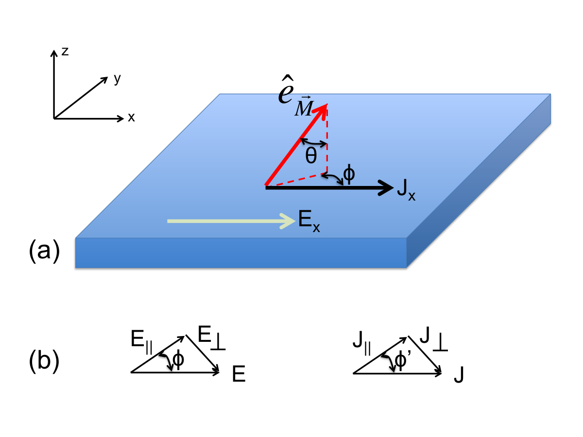
Here we derive phenomenologically the functional forms, which fit the computed longitudinal and transversal components of the residual resistivity tensor. The system of interest is an adatom with a tilted magnetic moment interacting with a gas of Rashba electrons. We assume a 2D current density flowing along the -direction, , that generates an electric field (see Fig.5(a)). Before analysing the general case of a tilted magnetic moment, let us recap what is expected when (i) the moment lies in-plane and (ii) the moment points out-of-plane. In case (i), we proceed as done by Thompson et al. [37] and consider the -component of :
| (62) |
where and are the components of the electric field parallel and perpendicular to the projection of the unit vector of the magnetic moment, , lying in the plane (the surface plane) as depicted in Fig.5(b). In terms of the current density and resistivity, the previous equation is then rewritten considering the parallel and perpendicular projection of the 2D current density on the direction of the magnetic moment:
| (63) |
as function of the azimutal angle . Also, knowing that (see Fig.5(b)) leads to:
| (64) |
Here, though, we give this expression in terms of the unit vector, , defining the orientation of the moment:
| (65) |
Our proposal is that in the general case of a tilted magnetic moment, the previous two equations involving holds. However, there is a missing contribution from the out-of-plane component of the magnetic moment. In the extreme case (ii), i.e. magnetic moment out-of-plane, we have:
| (66) |
and a simple generalization leads to:
| (67) |
As deduced from our numerical investigation, (see FIG. 4 (a)). This can be explained from FIG. 3 (b) for and FIG. 3 (c) for , where the allowed scattering processes are the same except for the interband scattering which flips the spin but does not change the direction of . The latter affects only the spin part of the response function, not the residual resistivity (charge part) that we compute. Therefore we get the same residual resistivity for and .
Now we can add up both contributions (i) and (ii) and find:
| (68) |
which simplifies into:
| (69) |
A similar approach can be used to derive the functional forms for the transversal part of the residual resistivity tensor. Here we address the -component of and again after starting from the form of Thompson et al.[37] for the case (i):
| (70) |
we end up with
| (71) |
Since there is no transversal resistivity in the case (ii), the contribution vanishes and we find:
| (72) |
References
- [1] E. I. Rashba, Sov. Phys. Solid State. 2, 1109 (1960).
- [2] Y.A. Bychkov, E.I. Rashba: J. Phys. C: Solid State Phys. 17, 6039 (1984).
- [3] S. LaShell, B. A. McDougall, and E. Jensen, Phys. Rev. Lett. 77, 3419 (1996).
- [4] F. Reinert, G. Nicolay, S. Schmidt, D. Ehm, and S. Hüfner, Phys. Rev. B 63, 115415 (2001).
- [5] G. Nicolay, F. Reinert, S. Hüfner, P. Blaha, PRB. 65, 033407 (2001).
- [6] M. Hoesch, M. Muntwiler, V. N. Petrov, M. Hengsberger, L. Patthey, M. Shi, M. Falub, T. Greber, and J. Osterwalder, Phys. Rev. B 69, 241401 (2004).
- [7] A. Tamai, W. Meevasana, P.D.C. King, C.W. Nicholson, A. de la Torre, E. Rozbicki, and F. Baumberger, Phys. Rev. B 87, 075113 (2013).
- [8] G. Bihlmayer, Yu. M. Koroteev, P. M. Echenique, E. V. Chulkov and S. Blügel, Surf. Sci. 600, 3888 (2006).
- [9] G. Bihlmayer, S. Blügel, and E. V. Chulkov, Phys. Rev. B 75, 195414 (2007).
- [10] C. R. Ast, G. Wittich, P. Wahl, R. Vogelgesang, D. Pacilé, M. C. Falub, L. Moreschini, M. Papagno, M. Grioni, and K. Kern, Phys. Rev. B 75, 201401(R) (2007).
- [11] D. Marchenko, A. Varykhalov, M. R. Scholz, G. Bihlmayer, E. I. Rashba, A. Rybkin, A. M. Shikin, and O. Rader, Nature Communications 3, 1232 (2012).
- [12] A. M. Shikin, A. A. Rybkina, A. S. Korshunov, Yu. B. Kudasov, N. V. Frolova, A. G. Rybkin D. Marchenko, J. Sanchez-Barriga, A. Varykhalov and O. Rader, New J. Phys. 15, 095005 (2013).
- [13] I. Gierz, T. Suzuki, E. Frantzeskakis, S. Pons, S. Ostanin, A. Ernst, J. Henk, M. Grioni, K. Kern, and C. R. Ast, Phys. Rev. Lett. 103, 046803 (2009).
- [14] V. M. Edelstein , Solid State Comm. 73, 233-235 (1990).
- [15] N. Nagaosa, J. Sinova, S. Onoda, A. H. MacDonald, and N. P. Ong, Rev. Mod. Phys. 82, 1539 (2010).
- [16] K. M. Seemann, Y. Mokrousov, A. Aziz, J. Miguel, F. Kronast, W. Kuch, M. G. Blamire, A. T. Hindmarch, B. J. Hickey, I. Souza, and C. H. Marrows, Phys. Rev. Lett. 104, 076402 (2010).
- [17] W. Thomson, Proc. Royal Soc. London 8, 546 (1857).
- [18] K. L. Yau and J. T. H. Chang, J. Phys. F.: Metal Phys. 1, 38 (1971).
- [19] K.M. Seemann, F. Freimuth, H. Zhang, S. Blügel, Y. Mokrousov, D.E. Bürgler, and C.M. Schneider, Phys. Rev. Lett. 107, 086603 (2011).
- [20] M. F. Crommie, C. P. Lutz, and D. M. Eigler, Nature 363, 524 (1993).
- [21] S. Lounis, A. Bringer, and S. Blügel, Phys. Rev. Lett. 108, 207202 (2012).
- [22] H. Ishida, Phys. Rev. B 52, 10819 (1995); H. Ishida, Phys. Rev. B 54, 10905 (1996).
- [23] M. I. Trioni, H. Ishida, and G. P. Brivio, Phys. Rev. B 65, 125413 (2002).
- [24] H. A. Engel, E. I. Rashba, and B. I. Halperin, Phys. Rev. Lett. 98, 036602 (2007).
- [25] P. Sengupta, and E. Bellotti, Journal of Physics: Condensed Matter 27, 405301 (2015).
- [26] J. Friedel, NuovoCimento Suppl. 7, 287 (1958).
- [27] J. D. Walls, J. Huang, R. M. Westervelt, and E. J. Heller, Phys. Rev. B 73, 035325 (2006).
- [28] G. A. Fiete, E. J. Heller, Rev. Mod. Phys. 75, 933 (2003).
- [29] S. Crampin, M. H. Boon, and J. E. Inglesfield, Phys. Rev. Lett. 73, 1015 (1994).
- [30] S. Crampin and O. R. Bryant, Phys. Rev. B 54, R17367 (1996).
- [31] H. K. Harbury and W. Porod, Phys. Rev. B 53, 15455 (1996).
- [32] Y. Hasegawa and P. Avouris, Phys. Rev. Lett. 71, 1071 (1993).
- [33] M. F. Crommie, C. P. Lutz, and D. M. Eigler, Science 262, 218 (1993).
- [34] E. J. Heller, M. F. Crommie, C. P. Lutz, and D. M. Eigler, Nature 369, 464 (1994).
- [35] S. Heers, Ph. Mavropoulos, S. Lounis, R. Zeller, and S. Blügel, Phys. Rev. B 86, 125444 (2012).
- [36] N. Papanikolaou, R. Zeller, and P. H. Dederichs, J. Phys: Condens. Matter 14, 2799 (2002).
- [37] D. A. Thompson, L. T. Romankiw, and A. F. Mayadas, IEEE Trans. Magn. 11, 1039 (1975).
- [38] M. Trushin, K. Výborný, P. Moraczewski, A. A. Kovalev, J. Schliemann, and T. Jungwirth, Phys. Rev. B 80, 134405 (2009).