This work was motivated by the successful use of the thermodynamic volume in studies of AdS black holes, and investigating whether this would also be the case for dS black holes. The volume $V$ was found to arise naturally in the Smarr relation and first law for AdS black holes as the variable conjugate to $\Lambda$ [49], and was then used in in studying isoperimetric inequalities [50]. Further research made use of $V$ in deriving various equations of state, and analyzing phase transitions for AdS black holes [51, 52, 53, 54, 55, 56, 57]. As in the earlier analysis of the Hawking-Page phase transition [58] and subsequent work which explored the extended AdS-black hole phase space [59, 60, 61], the temperature plays a key role. For example, studies of AdS black holes typically proceed by looking at the isotherms of the black holes in the pressure - volume phase space, where the pressure is provided by the cosmological constant

Critical temperatures and associated phase transitions can then be identified by seeing whether, or not, an isotherm develops extrema as a function of the temperature. Since AdS itself does not have a naturally specified temperature, the formalism of classical thermodynamic ensembles carries over to Euclidean AdS, where the Euclidean time period is fixed by the black hole temperature. The free energy can then be used to quantify properties of the phase transition.

For black holes in deSitter none of these tools carries over in a simple way. There are two temperatures, $T_{cos}$ and $T_{bh}$, associated with the cosmological and black hole horizons respectively, so it is not clear how to treat the system as a fluid with one temperature, or what temperature to use for a free energy. The Smarr formula and the first law (equations (3) and (4) below) treat each temperature and each horizon entropy on an equal footing. There are special cases when the two temperatures are equal, and in these cases, calculations of the Euclidean action give that it is equal to $(A_{ds}+A_{bh})/4$, that is, to the total horizon entropy [2, 4, 58, 12, 15, 14]. Very interestingly, recent calculations done for cases when the temperatures are not equal give the same result [37, 38]. These considerations lead us to use the entropy as the quantity to organize the properties of the black holes, rather than temperature, an approach which turns out to be quite useful.

When $\Lambda>0$ a Smarr formula for stationary charged black holes can be derived which only involves quantities on the black hole and cosmological horizons [48], which in $D=4$ is

where $J$ is the angular momentum, $Q$ is the charge, $S_{h}=A_{h}/4$, $\Omega_{h}$, and $T_{h}$ are the horizon entropies, rotational velocities, and temperatures respectively, and $\Phi=\phi_{bh}-\phi_{cos}$ is the electric potential difference between the two horizons. In our notation the temperatures are always positive with $2\pi T_{h}=|\kappa_{h}|$. The thermodynamic volume between the horizons $V$ is equal to $V_{cos}-V_{bh}$, the difference between the thermodynamic volumes associated with each of the cosmological and the black hole horizons separately. The mass does not appear since it subtracts out from two distinct Smarr relations which connect the black hole (cosmological) horizon to infinity. Similarly, the first law formulated in the region between the two horizons is [48]

These fundamental relations, which hold for any stationary Einstein-Maxwell-positive $\Lambda$ black hole spacetime, illustrate that there are more relevant thermodynamic quantities for dS than AdS. We now specialize to the known analytic KNdS metrics.

In $D=4$ the KNdS metric for a rotating, charged black hole with positive cosmological constant is [1]

where

The gauge field is $A=-qr/\rho^{2}(dt\!-{a\over\gamma}\sin^{2}\theta d\varphi)$. The ADM mass $M$, angular momentum $J$, and electric charge $Q$ are related to the metric parameters $m,a$ and $q$ by $M=m/\gamma^{2},\ J=am/\gamma^{2}$, and $Q=q/\gamma$. The angular velocities and the electric potential at each horizon is given by $\Omega_{h}=a\gamma/(r_{h}^{2}+a^{2}),\ \phi_{h}=qr_{h}/(r_{h}^{2}+a^{2})$. Details can be found in [12], and an analysis of the global spacetime structure is given in [45].

The horizon areas and the thermodynamic volumes associated with each of the black hole and the cosmological horizons are given by

One sees that $V_{cos}$ and $V_{bh}$ are not equal to their respective geometric volumes [50], but they differ by the same angular momentum dependent term. Hence, amazingly, the thermodynamic volume $V=V_{cos}-V_{bh}$ between the horizons is equal to the geometric volume [50],

The surface gravity at a horizon is given by $2\kappa_{h}=(r_{h}^{2}+a^{2})^{-1}\Delta^{\prime}(r_{h})$. The surface gravity is positive at the black hole horizon and negative at the deSitter horizon. We define the temperatures as the positive quantities $2\pi T_{bh}=\kappa_{bh}$ and $2\pi T_{cos}=-\kappa_{dS}$. The horizons $r_{h}$ occur at $\Delta(r_{h})=0$, which implies that at each horizon

Computing the temperatures and using (12) to eliminate $m$ gives

where the plus sign is for the black hole horizon $r_{bh}$, the minus sign is for $r_{cos}$, and

The KNdS spacetimes are a four parameter family, written above in terms of $(l,a,q,m)$. We next show that the system can be more readily analyzed if $m$ is traded for a different geometric parameter $X$, which we are lead to as follows. We define

Subtracting (12) for each of $r_{h}=r_{cos},\ r_{bh}$ gives

This becomes a relation for $V$ in terms of $X$ and $L$ by making use of (10) and (11),

The volume will be non-negative in the physical parameter space, which will be derived in Section (4). Next, note that the quantity $(r_{cos}-r_{bh})$ can be factored out of equation (16) yielding $(r_{cos}-r_{bh})^{2}=l^{2}-a^{2}-3r_{cos}r_{bh}-\tilde{a}^{2}/(r_{cos}r_{bh})$, or

We will view equation (18) as giving $L$ in terms of $X,q,a,l$, and so $V$ is also given as a function of these parameters in equation (17).

Since $X=r_{bh}(r_{bh}+L)$ the horizon radii are given in terms of $X$ by

where the minus sign is for $r_{bh}$ and the plus sign for $r_{cos}$. The horizon areas follow from the radii. Of particular interest in this work is the sum of the areas of the black hole and deSitter horizons, which has the simple form

Note that the total area is invariant under replacing $X$ with $\tilde{a}^{2}l^{2}/X$,

This symmetry will prove to be useful and interesting.

Lastly we find in terms of $l,a,q$, and $X$. Denote the inner black hole or Cauchy horizon as $r_{in}$ and the negative root as $r_{neg}$, so that $\Delta(r)$ factors as

Comparing to (7) and ,aking use of the expressions (19) for $r_{cos}$ and $r_{bh}$ gives

Hence the metric functions are now specified in terms of $l,a,q$ and $X$, so that $X$ replaces $m$ as the fourth metric parameter.

The main results of this section are the relations (17) through (23) which give thermodynamic quantities as functions of the physical parameters $l,a,q,$ and $X$.

The geometrical significance of $X$ is that it is related to the product of the horizon areas by

However, a reader might legitimately point out that each of $r_{cos}$ and $r_{bh}$ has a similar geometric significance so why should we go through the bother of introducing their product $X$? Good question! First, $X$ is only one parameter whereas the two radii would be a redundant set. Suppose one decides to use $r_{bh}$ along with $l,a,q$, and wants to graph the areas, temperatures, volume, and mass as functions of $l,a,q$ and $r_{bh}$. The area and temperature of the black hole horizon are given by direct substitution into (10 ) and (13). To find the other quantities one needs $r_{cos}$. Fixing $r_{bh}$ determines $m$ through $\Delta(r_{bh})=0$. Once $m$ is known one needs to solve the quartic equation $\Delta(r_{cos})=0$ to find $r_{cos}$. Therefore in order to plot, for example, the entropies as a function of $r_{bh}$, a quartic has to be solved for each value of $r_{bh}$. If one chooses $m$ as the fourth parameter rather than $r_{bh}$ the situation is worse - then a quartic needs to be solved to find each of $r_{bh}$ and $r_{cos}$. On the other hand, equations (18) through (23) give the thermodynamic quantities directly in terms of $l,a,q$ and $X$ and so can be plotted directly. Indeed, the total entropy (20) is simple enough to be accurately sketched using basic calculus.

Once the physical range of parameters is established (Section(4)) it is straightforward to show that $A_{bh}$ and $m$ are are monotonically related to $X$, so that qualitatively one can simply think of large $X$ as large $A_{bh}$ and vice-versa. Lastly, we note that the physically relevant range of $X$ will be found by algebra no more difficult than solving a quadratic. This is in contrast to the situation if the four horizon roots are used as parameters, in which case the physically allowed parameter space must be found numerically [14].

The temperature $T_{bh}$ ($T_{cos}$) is given as a function of $l,a,q$ and $r_{bh}$ ($r_{cos}$) in (13), so with the formula for the radii in equation (19) each temperature is known in terms of the four parameters $l,a,q,$ and $X$. This allows one to determine both temperatures for a given metric by simple substitution. Plots of the temperatures in some representative cases are given in Figure 1. Of special interest in the literature are the equal temperature solutions with $T_{cos}=T_{bh}$. This requires that $-(r_{bh}^{2}+a^{2})\Delta^{\prime}(r_{cos})=(r_{cos}^{2}+a^{2})\Delta^{\prime}(r_{bh})$. One finds that solutions occur when either $r_{cos}=r_{bh}$, which is when the two horizons coincide and the common temperature is zero, or $X^{2}-2a^{2}X-\tilde{a}^{2}l^{2}=0$, with positive solution

In the analysis of reference [8], which studied the charged, non-rotating system, these were referred to as “lukewarm” black holes. Not all choices of $(l,a,q)$ give values of $X_{eq}$ that are in the physical parameter space. As a result only in part of $(l,a,q)$ parameter space are there black holes with (non-zero) equal temperatures. Figure 1 gives plots of $T_{bh}$ and $T_{cos}$ as a function of $X$ in two representative cases from two different regions of parameter space. At the small $X$ side the black hole temperature starts at zero, which is the extremal black hole case where the black hole outer and inner horizons merge. At the large $X$ end $T_{cos}$ and $T_{bh}$ go to the common value of zero as the black hole and cosmological horizons approach each other. On the left hand side of Figure 1, $T_{bh}$ is always less than $T_{cos}$, whereas on the right hand side, there is an equal temperature spacetime, and then $T_{bh}$ is greater than $T_{cos}$ for $X>X_{eq}$.

With $a=0$ the equal temperature metrics occur when $M=Q$. In the general case the mass is given by substituting $X_{eq}$ into (23), but does not give such a simple result. When $\Lambda=0$ and $a=0$ the condition that the charge is equal to the mass occurs when the inner and outer black hole horizons coincide, with common temperature equal to zero. This situation admits multi-centered static black holes described by the Majumdar-Papepetrou metric [62], illustrating a gravitational-electromagnetic force balance. With $\Lambda>0$ and $a=0$, the charge equal to mass case corresponds to the black hole and cosmological temperatures being equal and non-zero. Further, $Q=M$ still describes a kind of force balance situation - the ground state condition was exploited to find multi-centered cosmological $Q=M$ black holes in [63], which is a time dependent generalization of the $Q=M$ Majumbar-Papepetrou spacetimes. It would be very interesting to find a multi- rotating and charged black hole cosmology, possibly corresponding to the equal temperature situation, but to our knowledge an analytic solution has not yet been found.

In this section we find the constraints on the parameters $l,a,q$, and $X$ so that the metric (5) describes an asymptotically deSitter black hole. One requires that the spacetime has cosmological, black hole, and inner Cauchy horizons, and that the coordinate $t$ is timelike between the black hole and cosmological horizons. In the form of the KNdS metric (5) this means that $\Delta(r)\geq 0$ for $r_{bh}\leq r\leq r_{cos}$ and that $T_{bh/cos}\geq 0$. Such an analysis is carried out in reference [14] by finding restrictions on the four roots $r_{h}$ to $\Delta(r_{h})=0$, and then translating the allowed parameter space for the roots to the physical parameter space for $l,a,q$, and $m$. This involves a combination of algebraic and numerical work, resulting in the elegant plot displayed in Figure 2 of that paper.

Here we will be able to proceed more directly. Consulting equation (19) we see that the horizon radii are positive real quantities if $X\geq 0$, $L^{2}\geq 0$, and we define $L$ to be the positive square root of $L^{2}$. We next impose these conditions, plus the condition $T_{bh/cos}\geq 0$, and map out the complete parameter space of $a,q,$ and $X$ for a given value of $l$. The quantity $L^{2}$ given in equation (18) can be factored as $L^{2}=(X-X_{L-})(X_{L+}-X)/X$ where

Here $X_{L\pm}$ denote the zeros of $L^{2}$, which are real and positive as long as $1-a^{2}/l^{2}>0$ and $(1-a^{2}/l^{2})^{2}-12(\tilde{a}/l)^{2}\geq 0$. The second inequality implies the first. The case of equality defines the elliptical-like curve $12{q^{2}\over l^{2}}+14{a^{2}\over l^{2}}-{a^{4}\over l^{4}}=1$ and the allowed points $p=(a/l,q/l)$ in the parameter space ${\cal P}$ lie in the interior of, or on, this curve. Rewriting this relation in factored form gives

Hence the largest that $a/l$ can be is $(2-\sqrt{3})$. We will see in a moment that the additional condition that the temperatures are positive does not further restrict $l,a,q$, so ${\cal P}$ is the allowed parameter space of $(l,a,q)$. Hence if $X_{L-}\leq X\leq X_{L+}$ and $(a,q,l)$ belong to ${\cal P}$ then $X$ and $L^{2}$ are real and non-negative. This ensures that the roots satisfy $r_{cos}\geq r_{bh}\geq 0$.

In order that the metric function $\Delta(r)$ be positive between $r_{bh}$ and $r_{cos}$, we need to check that $T_{bh},\ T_{cos}\geq 0$. Equation (13) for the temperatures can be written as

were the minus (plus) sign is for the black hole (cosmological) temperature. It is straightforward to check that assuming $L^{2}>0$, if $T_{bh}>0$ then $T_{cos}>0$. Hence it is sufficient to determine the conditions for $T_{bh}>0$. Assuming that $L^{2}>0$, then equation (36) implies that $r_{bh}^{2}$ must lie in the range $X_{L-}\leq r_{bh}^{2}\leq X_{L+}$. Pursuing some algebra and using (19) for $r_{bh}$, one finds that $T_{bh}\geq 0$ when $(X-X_{T-})(X_{T+}-X)\geq 0$, where

Since $X_{L-}<X_{T-}$ and $X_{L+}<X_{T+}$, requiring both $L^{2}\geq 0$ and positive temperatures gives the allowed range of $X$,

To have any values in this range it is necessary that

What is the physics of the range on $X$? At the lower end, the black hole temperature vanishes but $L$ does not. Hence this is an extremal black hole where the inner and event horizons coincide, but the cosmological and black hole event horizons are distinct. At the upper end, $L^{2}$ is zero, so the black hole and deSitter horizons merge with the temperature of each going to zero.

To summarize, the physical parameter space for KNdS black holes is given by $X$ in the interval $R_{p}$ and $(a/l,q/l)$ in ${\cal P}$, specified in equations (38) and (35) respectively. Note that the $3$-dimensional parameter space ${\cal P}\times R_{p}$ is scale-invariant with respect to $l$, consistent with the fact that the $l$ dependence of the metric simply appears as a conformal factor $l^{2}$, if the coordinates and parameters are rescaled in units of $l$.

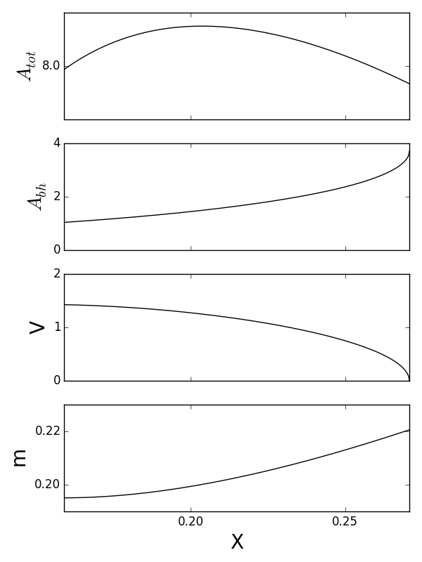
The horizon radii, volume, and mass are then functions on this space given in (19), (17), and (23). It is helpful to look at Figure 2, which shows that in the allowed range of $X$ the black hole area and the mass increase monotonically with $X$ while the volume decreases. So as we discuss subsequent relations one can think of larger $X$ as larger area black holes and vice-versa.

In this section we study properties of the total entropy $S={1\over 4}A_{tot}$. We will see that the parameter space ${\cal P}$ can be divided into regions according to qualitative features of the total entropy $S$. The results are summarized in Figure 3, and we turn to the derivation of this diagram.

One can read off of equation (20) that the entropy has the intriguing property that it is invariant under the map

The maximum of $A_{tot}$ occurs at $X_{crit}=\tilde{a}l$, which is the fixed point of this map. Hence for values of $A_{tot}$ less than the maximum, two distinct values of $X$ will have the same total entropy. However, whether, or not, these values of $X$ correspond to physical black hole spacetimes depends on whether they are both in the allowed range for $X$ specified in equation (38), at the values of $(a/l,q/l)$ under consideration. Hence our next step is to figure out the structure imposed on the parameter space ${\cal P}\times R_{p}$ by the behavior of $S$. Specifically, let $S_{p}$ be the set of values of the entropy that are obtained by KNdS black holes at $p$. The map

is either one-to-one or one-to-two. If $\psi$ is 1-1 at $p$ then for each value of the entropy in $S_{p}$ there is a unique black hole. When $\psi_{p}$ is 1-2, then there are two black hole spacetimes that have that have the same value $S$, that is, there are degenerate entropy states. We will refer to this behavior as unique black holes ${\cal U}$, large black holes are degenerate ${\cal LD}$, or small black holes are degenerate ${\cal SD}$, according to whether $\psi_{p}$ is 1-1 on the entire range of $X$, 1-2 for large $X$ and hence for large black holes, or 1-2 for small $X$ and hence for small black holes. These different behaviors of $A_{tot}$ as a function of $X$, depending on the value of $(a/l,q/l)$, are illustrated in Figures 4 and 5.

The regions in ${\cal P}$ divide nicely into rings, with the boundaries of the rings corresponding to special configurations, which are determined as follows. Using $X_{L+}X_{L-}=\tilde{a}^{2}l^{2}/3$ and equation (37) gives $X_{T-}$ in terms of $X_{L+}$, and implies that $X_{T-}\leq\tilde{a}l$. Since the maximum of $S$ occurs at $X=\tilde{a}l$, there will be degeneracy at $p$ for some $X$ if $\tilde{a}l\leq X_{L+}$ at $p$.

The smallest possible range of $X$ is the single value $X=X_{T-}=X_{L+}=\tilde{a}l/\sqrt{3}$. Using the expressions for $X_{T-}$ and $X_{L+}$ in equations (34) and (37) one finds that $(a/l,q/l)$ must satisfy $(1-a^{2}/l^{2})^{2}-12(\tilde{a}/l)^{2}=0$ which is just the boundary of the total parameter space ${\cal P}$. Hence all the KNdS spacetimes on $\partial{\cal P}$ have the same value of $X$. By continuity one expects that for some range of $X_{L+}$ near $\tilde{a}l/\sqrt{3}$ the entropy will likewise correspond to a unique black hole, so we want to find the inner boundary of the set ${\cal U}$ within ${\cal P}$ that consists of black holes which are uniquely specified by $S$ and $p$. By the remarks in the previous paragraph, the inner boundary of ${\cal U}$ is determined by the condition $\tilde{a}l=X_{L+}$, which translates into the curve

Points $p$ inside this curve will have a range of $X$ values that include both unique and degenerate entropy states. Moving just inside $\partial{\cal U}$ one finds that the degenerate states occur at the larger values of $X$, which are larger area black holes and are denoted ${\cal LD}$. The region at the center of ${\cal P}$ contains the points at which the degenerate states occur at small $X$, which are smaller area black holes, or ${\cal SD}$. The boundary curve between the large and small degenerate states is when all $X$ values have isentropic partners. This occurs when the endpoints are dual to each other satisfying $X_{L+}^{\prime}=X_{T-}$. One finds that this condition becomes $X_{L+}=\sqrt{{5}\over 3}\tilde{a}l$ and the curve in ${\cal P}$ on which all states are degenerate is

Collecting these results, we have the following division of the parameter space ${\cal P}$:

$\underline{\partial{\cal P}:}\ \ X_{T-}=X_{L+}=\tilde{a}l/\sqrt{3}$ In this case the range of $X$ has shrunk to one value, indicating that the three horizons coincide and the temperatures are zero. This configuration was called the “ultra extreme black hole” in the analysis of coinciding horizons of charged black holes in deSitter [44]. The algebraic equation for the perimeter is given by the boundary of (35).

$\underline{{\cal U}:\ Unique\ states:}\quad\tilde{a}l/\sqrt{3}<\ X_{T-},\ X_{T+}<\ \tilde{a}l$. The upper limit for $X$ is less than where the area curve reaches a maximum. All black holes have a unique value of $S$. ($\psi$ is 1-1 on $R_{p}$.) The inner boundary is given by the curve (42), See Figure 4.

$\underline{{\cal LD}:\ Large\ Degenerate:}\quad\tilde{a}l/\sqrt{3}<\ X_{T-},\ \tilde{a}l\ <X_{T+}<\ \sqrt{5\over 3}\tilde{a}l$. The upper limit for $X$ has increased to include the value where $S$ is maximum. All large black holes are dual to a smaller black hole with the same $S$. ($\psi$ is 1-1 at small $X$ and is 2-1 at large $X$ on $R_{p}$.) See Figure 4.

$\underline{\partial{(\cal LS}):\ All\ Degenerate:}\quad X_{T-}=\sqrt{3\over 5}\tilde{a}l,\ X_{L+}=\ \sqrt{5\over 3}\tilde{a}l$. At the boundary between ${\cal LD}$, where large black holes are degenerate but not all the small ones are, and ${\cal SD}$, where small black holes are degenerate but not all the large ones are, is the balanced situation when every black hole is dual to another black hole. ($\psi$ is 1-2 on $R_{p}$.) The equation for this curve is given in (43). See Figure 5.

$\underline{{\cal SD}:\ Small\ Degenerate:}\quad\sqrt{3\over 5}\tilde{a}l<X_{T-}<\tilde{a}l,\ \sqrt{5\over 3}\tilde{a}l\ <X_{L+}$. The upper and lower limits for $X$ have increased so that some large black holes no longer have dual states. All small black holes are dual to a larger black hole with the same $S$. ($\psi$ is 1-2 at small $X$ and is 1-1 at large $X$ on $R_{p}$.) See Figure 5.

The structure of ${\cal P}$ is summarized in Figure 3, which we see splits neatly into rings that delineate whether each value of the entropy corresponds to a unique KNdS black hole, or if some values of $S$ correspond to two black holes. The graphs in Figure 2 illustrate that the mass and the area of the black hole horizon are monotonically related to area product $X$. For $a=q=0$ it simple to show that $m$ and $A_{bh}$ increase monotonically with $X$ and with each other. A more tedious, but straightforward, calculation shows that when $a$ and $q$ are nonzero it is still the case that $A_{bh}$ and $m$ increase monotonically with $X$, in the physical parameter space. Hence black holes with large areas do indeed correspond to black holes with large mass, and when reading plots with independent variable $X$ one can think of increasing $X$ as increasing black hole area and mass.

In classical thermodynamics, a system evolves to maximize its entropy, and in equilibrium, the components of a system have the same temperature. The thermodynamic properties of charged deSitter black holes with no rotation are consistent with our non-gravitating thermodynamic expectations, as the equal temperature black holes are also maximum entropy black holes. These occur when $X=ql$ and satisfy $m=q$. However, when rotation is added these these two properties no longer coincide. The maximum of the entropy occurs at $X_{maxS}=\tilde{a}l$ which does not equal $X_{eq}$ given in equation (25) unless $a=0$. At the maximum entropy black hole the mass is given by

where we have explicitly written out the charge dependence to highlight how $m=q$ generalizes when $a$ is non-zero. The first factor is the “norm” of the conserved charges, and the second factor has the form of a gravitational redshift. So when considering what physics of the KNdS metrics persist in a situation like inflation when $\Lambda$ is actually dynamical, it may be that maximizing $S$, or evolving to equal temperatures, or some compromise between the two, is the key principle.

References

- [1] B. Carter, in ”Black Holes”, ed C DeWitt and B S DeWitt (New York: Gordon and Breach).
- [2] G. W. Gibbons and S. W. Hawking, “Action Integrals and Partition Functions in Quantum Gravity,” Phys. Rev. D 15, 2752 (1977).
- [3] G. W. Gibbons and S. W. Hawking, “Cosmological Event Horizons, Thermodynamics, and Particle Creation,” Phys. Rev. D 15, 2738 (1977).
- [4] G. W. Gibbons and S. W. Hawking, “Classification of Gravitational Instanton Symmetries,” Commun. Math. Phys. 66, 291 (1979).
- [5] P. C. W. Davies, “Cosmological Horizons and the Generalized Second Law of Thermodynamics,” Class. Quant. Grav. 4, L225 (1987).
- [6] P. C. W. Davies, “Thermodynamic Phase Transitions of Kerr-Newman Black Holes in De Sitter Space,” Class. Quant. Grav. 6, 1909 (1989).
- [7] J. Guven and D. Nunez, Phys. Rev. D42, 2577, (1990).
- [8] L. J. Romans, “Supersymmetric, cold and lukewarm black holes in cosmological Einstein-Maxwell theory,” Nucl. Phys. B 383, 395 (1992) [hep-th/9203018].
- [9] A. M. Ghezelbash and R. B. Mann, “Entropy and mass bounds of Kerr-de Sitter spacetimes,” Phys. Rev. D 72, 064024 (2005) [hep-th/0412300].
- [10] Y. Sekiwa, Thermodynamics of de Sitter black holes: Thermal cosmological constant, Phys.Rev. D73 (2006) 084009, [hep-th/ 0602269].
- [11] D. Anninos and T. Anous, “A de Sitter Hoedown,” JHEP 1008, 131 (2010) [arXiv:1002.1717 [hep-th]].
- [12] F. Mellor and I. Moss, “Black Holes and Gravitational Instantons,” Class. Quant. Grav. 6, 1379 (1989).
- [13] R. B. Mann and S. F. Ross, “Cosmological production of charged black hole pairs,” Phys. Rev. D 52, 2254 (1995) [gr-qc/9504015].
- [14] I. S. Booth and R. B. Mann, “Cosmological pair production of charged and rotating black holes,” Nucl. Phys. B 539, 267 (1999) [gr-qc/9806056].
- [15] I. S. Booth and R. B. Mann, “Complex instantons and charged rotating black hole pair creation,” Phys. Rev. Lett. 81, 5052 (1998) [gr-qc/9806015].
- [16] O. J. C. Dias and J. P. S. Lemos, “Pair creation of de Sitter black holes on a cosmic string background,” Phys. Rev. D 69, 084006 (2004) [hep-th/0310068].
- [17] O. J. C. Dias, “Pair creation of anti-de Sitter black holes on a cosmic string background,” Phys. Rev. D 70, 024007 (2004) [hep-th/0401069].
- [18] F. Mellor and I. Moss, “Stability of Black Holes in De Sitter Space,” Phys. Rev. D 41, 403 (1990).
- [19] S. Yoshida, N. Uchikata and T. Futamase, “Quasinormal modes of Kerr-de Sitter black holes,” Phys. Rev. D 81, 044005 (2010).
- [20] A. Strominger, “The dS / CFT correspondence,” JHEP 0110, 034 (2001) [hep-th/0106113].
- [21] R.-G. Cai, Cardy-Verlinde formula and asymptotically de Sitter spaces, Phys.Lett. B525 (2002) 331–336, [hep-th/0111093].
- [22] R.-G. Cai, Cardy-Verlinde formula and thermodynamics of black holes in de Sitter spaces, Nucl.Phys. B628 (2002) 375–386, [hep-th/0112253].
- [23] A. M. Ghezelbash and R. B. Mann, “Action, mass and entropy of Schwarzschild-de Sitter black holes and the de Sitter / CFT correspondence,” JHEP 0201, 005 (2002) [hep-th/0111217].
- [24] R. Bousso, A. Maloney and A. Strominger, “Conformal vacua and entropy in de Sitter space,” Phys. Rev. D 65, 104039 (2002) [hep-th/0112218].
- [25] J. l. Jing, “Cardy-Verlinde formula and entropy bounds in Kerr-Newman AdS(4) / dS(4) black hole backgrounds,” Phys. Rev. D 66, 024002 (2002) [hep-th/0201247].
- [26] V. Balasubramanian, J. de Boer and D. Minic, “Notes on de Sitter space and holography,” Class. Quant. Grav. 19, 5655 (2002) [Annals Phys. 303, 59 (2003)] [hep-th/0207245].
- [27] A. Guijosa and D. A. Lowe, “A New twist on dS / CFT,” Phys. Rev. D 69, 106008 (2004) [hep-th/0312282].
- [28] M. R. Setare, “The Cardy-Verlinde formula and entropy of black holes in de Sitter spaces,” TSPU Bulletin 44N7, 5 (2004) [hep-th/0405010].
- [29] A. Guijosa, D. A. Lowe and J. Murugan, “A Prototype for dS/CFT,” Phys. Rev. D 72, 046001 (2005) [hep-th/0505145].
- [30] B. Chen and J. Long, “On Holographic description of the Kerr-Newman-AdS-dS black holes,” JHEP 1008, 065 (2010) [arXiv:1006.0157 [hep-th]].
- [31] B. Chen, C. M. Chen and B. Ning, “Holographic Q-picture of Kerr-Newman-AdS-dS Black Hole,” Nucl. Phys. B 853, 196 (2011) [arXiv:1010.1379 [hep-th]]
- [32] X. Xiao, “Holographic representation of local operators in de sitter space,” Phys. Rev. D 90, no. 2, 024061 (2014) [arXiv:1402.7080 [hep-th]].
- [33] T. Anous, D. Z. Freedman and A. Maloney, “de Sitter Supersymmetry Revisited,” JHEP 1407, 119 (2014) [arXiv:1403.5038 [hep-th]].
- [34] A. Chatterjee and D. A. Lowe, “Holographic operator mapping in dS/CFT and infrared divergences,” arXiv:1503.07482 [hep-th].
- [35] D. Sarkar and X. Xiao, “Holographic Representation of Higher Spin Gauge Fields,” Phys. Rev. D 91, no. 8, 086004 (2015) [arXiv:1411.4657 [hep-th]].
- [36] D. Sarkar, “(A)dS holography with a cutoff,” Phys. Rev. D 90, no. 8, 086005 (2014) [arXiv:1408.0415 [hep-th]].
- [37] R. Gregory, I. G. Moss and B. Withers, “Black holes as bubble nucleation sites,” JHEP 1403, 081 (2014) [arXiv:1401.0017 [hep-th]].
- [38] P. Burda, R. Gregory and I. Moss, “Gravity and the stability of the Higgs vacuum,” arXiv:1501.04937 [hep-th].
- [39] P. Burda, R. Gregory and I. Moss, “Vacuum metastability with black holes,” arXiv:1503.07331 [hep-th]
- [40] D. N. Page and S. W. Hawking, “Gamma rays from primordial black holes,” Astrophys. J. 206, 1 (1976).
- [41] B. J. Carr, “Some cosmological consequences of primordial black-hole evaporations,” Astrophys. J. 206, 8 (1976).
- [42] J. D. Barrow, E. J. Copeland and A. R. Liddle, “The Evolution of black holes in an expanding universe,” Mon. Not. Roy. Astron. Soc. 253, 675 (1991).
- [43] B. J. Carr and J. E. Lidsey, “Primordial black holes and generalized constraints on chaotic inflation,” Phys. Rev. D 48, 543 (1993).
- [44] D. R. Brill and S. A. Hayward, “Global structure of a black hole cosmos and its extremes,” Class. Quant. Grav. 11, 359 (1994) [gr-qc/9304007].
- [45] S. Akcay and R. A. Matzner, “Kerr-de Sitter Universe,” Class. Quant. Grav. 28, 085012 (2011) [arXiv:1011.0479 [gr-qc]].
- [46] A. Ashtekar, B. Bonga and A. Kesavan, “Asymptotics with a positive cosmological constant: I. Basic framework,” Class. Quant. Grav. 32, no. 2, 025004 (2015) [arXiv:1409.3816 [gr-qc]].
- [47] G. W. Gibbons, H. Lu, D. N. Page and C. N. Pope, “The General Kerr-de Sitter metrics in all dimensions,” J. Geom. Phys. 53, 49 (2005) [hep-th/0404008].
- [48] B. P. Dolan, D. Kastor, D. Kubiznak, R. B. Mann and J. Traschen, “Thermodynamic Volumes and Isoperimetric Inequalities for de Sitter Black Holes,” Phys. Rev. D 87, no. 10, 104017 (2013) [arXiv:1301.5926 [hep-th]].
- [49] D. Kastor, S. Ray and J. Traschen, “Enthalpy and the Mechanics of AdS Black Holes,” Class. Quant. Grav. 26, 195011 (2009) [arXiv:0904.2765 [hep-th]].
- [50] M. Cvetic, G. W. Gibbons, D. Kubiznak and C. N. Pope, “Black Hole Enthalpy and an Entropy Inequality for the Thermodynamic Volume,” Phys. Rev. D 84, 024037 (2011) [arXiv:1012.2888 [hep-th]].
- [51] B. P. Dolan, “The cosmological constant and the black hole equation of state,” Class. Quant. Grav. 28, 125020 (2011) [arXiv:1008.5023 [gr-qc]].
- [52] B. P. Dolan, “Pressure and volume in the first law of black hole thermodynamics,” Class. Quant. Grav. 28, 235017 (2011) [arXiv:1106.6260 [gr-qc]].
- [53] D. Kubiznak and R. B. Mann, “P-V criticality of charged AdS black holes,” JHEP 1207, 033 (2012) [arXiv:1205.0559 [hep-th]].
- [54] N. Altamirano, D. Kubiznak, and R. B. Mann, Reentrant phase transitions in rotating antide Sitter black holes, Phys.Rev. D88 (2013), no. 10 101502, [hep-th/ 1306.5756]
- [55] N. Altamirano, D. Kubiznak, R. B. Mann, and Z. Sherkatghanad, Kerr-AdS analogue of triple point and solid/liquid/gas phase transition, Class.Quant.Grav. 31 (2014) 042001, [hep-th/ 1308.2672]
- [56] N. Altamirano, D. Kubiznak, R. B. Mann, and Z. Sherkatghanad, Thermodynamics of rotating black holes and black rings: phase transitions and thermodynamic volume, Galaxies 2 (2014) 89–159, [hep-th/ 1401.2586].
- [57] B. P. Dolan, “Black holes and Boyle’s law Ñ The thermodynamics of the cosmological constant,” Mod. Phys. Lett. A 30, no. 03n04, 1540002 (2015) [arXiv:1408.4023 [gr-qc]].
- [58] S. W. Hawking and D. N. Page, “Thermodynamics of Black Holes in anti-De Sitter Space,” Commun. Math. Phys. 87, 577 (1983).
- [59] M. M. Caldarelli, G. Cognola and D. Klemm, “Thermodynamics of Kerr-Newman-AdS black holes and conformal field theories,” Class. Quant. Grav. 17, 399 (2000) [hep-th/9908022].
- [60] A. Chamblin, R. Emparan, C. V. Johnson, and R. C. Myers, Charged AdS black holes and catastrophic holography, Phys.Rev. D60 (1999) 064018, [hep-th/9902170].
- [61] A. Chamblin, R. Emparan, C. V. Johnson, and R. C. Myers, Holography, thermodynamics and fluctuations of charged AdS black holes, Phys.Rev. D60 (1999) 104026, [hep-th/9904197].
- [62] S. D. Majumdar, Phys. Rev. 72, 930 (1947); A. Papepetrou, Proc. Roy. Irish Acad. A51, 191 (1947).
- [63] D. Kastor and J. H. Traschen, “Cosmological multi - black hole solutions,” Phys. Rev. D 47, 5370 (1993) [hep-th/9212035].
- [64] M. Urano, A. Tomimatsu, and H. Saida, Mechanical First Law of Black Hole Spacetimes with Cosmological Constant and Its Application to Schwarzschild-de Sitter Spacetime, Class.Quant.Grav. 26 (2009) 105010, [hep-th/ 0903.4230].
- [65] M.-S. Ma, H.-H. Zhao, L.-C. Zhang, and R. Zhao, Existence condition and phase transition of Reissner-Nordström-de Sitter black hole, Int.J.Mod.Phys. A29 (2014) 1450050, [hep-th/ 1312.0731].
- [66] R. Zhao, M. Ma, H. Zhao, and L. Zhang, The Critical Phenomena and Thermodynamics of the Reissner-Nordstrom-de Sitter Black Hole, Adv.High Energy Phys. 2014 (2014) 124854.
- [67] H.-H. Zhao, L.-C. Zhang, M.-S. Ma, and R. Zhao, P-V criticality of higher dimensional charged topological dilaton de Sitter black holes, Phys.Rev. D90 (2014), no. 6 064018.
- [68] M.-S. Ma, L.-C. Zhang, H.-H. Zhao, and R. Zhao, Phase transition of the higher dimensional charged Gauss-Bonnet black hole in de Sitter spacetime, Adv.High Energy Phys. 2015 (2015) 134815, [hep-th/ 1410.5950].
- [69] X. Guo, H. Li, L. Zhang, and R. Zhao, Thermodynamics and phase transition in the Kerrde Sitter black hole, Phys.Rev. D91 (2015), no. 8 084009.
- [70] D. Kubiznak and F. Simovic, “Thermodynamics of horizons: de Sitter black holes,” arXiv:1507.08630 [hep-th].
- [71] Kerr-Newmann-deSitter Black Holes, [https://www.youtube.com/watch?v=lc70u1aWP8w ].
- [72] B. P. Dolan, “The compressibility of rotating black holes in D-dimensions,” Class. Quant. Grav. 31, 035022 (2014) [arXiv:1308.5403 [gr-qc]].
- [73] S. Chadburn and R. Gregory, “Time dependent black holes and scalar hair,” Class. Quant. Grav. 31, no. 19, 195006 (2014) [arXiv:1304.6287 [gr-qc]].
- [74] D. Kastor and J. H. Traschen, “Particle production and positive energy theorems for charged black holes in De Sitter,” Class. Quant. Grav. 13, 2753 (1996) [gr-qc/9311025].
- [75] D. Garfinkle, G. T. Horowitz and A. Strominger, “Charged black holes in string theory,” Phys. Rev. D 43, 3140 (1991) [Phys. Rev. D 45, 3888 (1992)].
- [76] F. Dowker, J. P. Gauntlett, D. A. Kastor and J. H. Traschen, “Pair creation of dilaton black holes,” Phys. Rev. D 49, 2909 (1994) [hep-th/9309075].
- [77] H. Friedrich, “On the existence of n-geodesically complete or future complete solutions of EinsteinÕs field equations with smooth asymptotic structure,” Comm. Math. Phys 107, 587 (1986).
- [78] L. Andersson and V. Moncrief, “Future complete vacuum spacetimes”. In: “The Einstein equations and the large scale behavior of gravitational fields.” Birkh?auser, Basel (2004).
- [79] H. Ringstrom, “Future stability of the Einstein-Non-Linear scalar field system,” Invent. Math. 173, 123(2008).
- [80] H. Ringstrom. “Power law inflation, ” Commun. Math. Phys. 290, 155 (2009).
- [81] X. Luo and J. Isenberg, “Power Law Inflation with Electromagnetism,” Annals Phys. 334, 420 (2013) [arXiv:1210.7566 [gr-qc]].
- [82] N. Fang et. al.,Nat. Mat. 5, 452 (2006).
- [83] C. Ding et. al., J. Appl. Phys.,108, 074911 (2010).