Recovering a stochastic process from noisy ensembles of many single particle trajectories

The physical motion of a stochastic particle is modeled by the Smoluchowski’s limit of the Langevin equation resulting in the equation of motion

$\displaystyle\dot{\mbox{\boldmath$X$}}=\mbox{\boldmath$a$}(\mbox{\boldmath$X$})+\mbox{\boldmath$b$}(\mbox{\boldmath$X$})\dot{\mbox{\boldmath$w$}},$

(1)

where $a$ is a deterministic drift, $b$ the diffusion tensor and $w$ the classical Wiener $\delta$-correlated noise. The Ito’s integral leads to

$\displaystyle\mbox{\boldmath$X$}(t)=\mbox{\boldmath$X$}(u)+\int_{u}^{t}\mbox{\boldmath$a$}(\mbox{\boldmath$X$}(s))ds+\int_{u}^{t}\mbox{\boldmath$b$}(\mbox{\boldmath$X$}(s))d\mbox{\boldmath$w$}_{s}$

(2)

and at times $0,\Delta t,\dots,n\Delta t$,

	$\displaystyle\int_{n\Delta t}^{(n+1)\Delta t}\mbox{\boldmath$a$}(X(s))ds$	$\displaystyle=$	$\displaystyle\mbox{\boldmath$a$}(\mbox{\boldmath$X$}_{n})\Delta t+o(\Delta t)$		(3)
	$\displaystyle\int_{n\Delta t}^{(n+1)\Delta t}\mbox{\boldmath$b$}(\mbox{\boldmath$X$}(s))d\mbox{\boldmath$w$}_{s}$	$\displaystyle=$	$\displaystyle\mbox{\boldmath$b$}(\mbox{\boldmath$X$}_{n})\Delta w,$		(4)

the discrete approximation sequence is

$\displaystyle\mbox{\boldmath$X$}_{n+1}=\mbox{\boldmath$X$}_{n}+\mbox{\boldmath$a$}(\mbox{\boldmath$X$}_{n})\Delta t+\mbox{\boldmath$b$}(\mbox{\boldmath$X$}_{n})\Delta w,$

(5)

where $\mbox{\boldmath$X$}_{n}=\mbox{\boldmath$X$}(n\Delta t)$.

We assume that the physical motion is sampled at points $\mbox{\boldmath$X$}_{n}$: at each time step, an additive Gaussian noise is added and the observed motion is described by

$\displaystyle\mbox{\boldmath$Y$}_{n}=\mbox{\boldmath$X$}_{n}+\mbox{\boldmath$Z$}_{n},\mbox{ where }\mbox{\boldmath$Z$}_{n}=\sigma{\mbox{\boldmath$\eta$}_{n}}$

(6)

and ${\mbox{\boldmath$\eta$}_{n}}$ is a $n$-dimensional Gaussian variable. We shall present various statistical parametric and non-parametric approaches to recover the underlying stochastic component of the continuous variable $X$ from the empirical measured sequence $\mbox{\boldmath$Y$}_{n}$.

We compute here the transition probability $p(\mbox{\boldmath$y$},n+1|\mbox{\boldmath$x$},n)=Pr\{\mbox{\boldmath$Y$}_{n+1}=\mbox{\boldmath$y$}|\mbox{\boldmath$Y$}_{n}=\mbox{\boldmath$x$}\}$ in one dimension when the diffusion tensor $b(X_{n})=\sqrt{2D}$ is uniform:

$\displaystyle p(Y_{n+1}=y|Y_{n}=x)$

$\displaystyle=$

$\displaystyle p(X_{n+1}+Z_{n+1}=y|X_{n}+Z_{n}=x).$

(7)

The two processes $X_{n}$ and $Z_{n}$ are independent and in ℝ, we have

	$\displaystyle p(Y_{n+1}=y|Y_{n}=x)$	$\displaystyle=$	$\displaystyle\int\limits_{\mathbb{R}}p(X_{n+1}+Z_{n+1}=y|X_{n}=x_{1})p(Z_{n}=x-x_{1})dx_{1}$
		$\displaystyle=$	$\displaystyle\int\limits_{\mathbb{R}}\int\limits_{\mathbb{R}}p(X_{n+1}=y_{1},Z_{n+1}=y-y_{1}|X_{n}=x_{1})p(Z_{n}=x-x_{1})dx_{1}dy_{1}$
		$\displaystyle=$	$\displaystyle\int\limits_{\mathbb{R}}\int\limits_{\mathbb{R}}p(X_{n+1}=y_{1}|X_{n}=x_{1})p(Z_{n+1}=y-y_{1})p(Z_{n}=x-x_{1})dx_{1}dy_{1}$
		$\displaystyle=$	$\displaystyle\int\limits_{\mathbb{R}}\int\limits_{\mathbb{R}}p(X_{n+1}=y_{1}|X_{n}=x_{1}).\frac{e^{-\displaystyle{\frac{(x-x_{1})^{2}}{2\sigma^{2}}}}}{\sigma\sqrt{2\pi}}\frac{e^{-\displaystyle{\frac{(y-y_{1})^{2}}{2\sigma^{2}}}}}{\sigma\sqrt{2\pi}}dx_{1}dy_{1}.$

For $\Delta t\ll 1$ and $X_{n+1}-X_{n}\sim\mathcal{N}(a(X_{n})\Delta t,\sqrt{2D\Delta t})$, the pdf is

$\displaystyle p(X_{n+1}=y_{1}|X_{n}=x_{1})=\frac{e^{-\displaystyle{\frac{(y_{1}-x_{1}-a(x_{1})\Delta t)^{2}}{4D\Delta t}}}}{\sqrt{4\pi D\Delta t}},$

(9)

which gives that

	$\displaystyle p(Y_{n+1}=y|Y_{n}=x)$	$\displaystyle=$	$\displaystyle\int\limits_{\mathbb{R}}\int\limits_{\mathbb{R}}\frac{e^{-\displaystyle{\frac{(y_{1}-x_{1}-a(x_{1})\Delta t)^{2}}{4D\Delta t}}}}{\sqrt{4\pi D\Delta t}}\frac{e^{-\displaystyle{\frac{(x-x_{1})^{2}}{2\sigma^{2}}}}}{\sigma\sqrt{2\pi}}\frac{e^{-\displaystyle{\frac{(y-y_{1})^{2}}{2\sigma^{2}}}}}{\sigma\sqrt{2\pi}}dx_{1}dy_{1}$
		$\displaystyle=$	$\displaystyle\int\limits_{\mathbb{R}}\frac{e^{-\displaystyle{\frac{(x-x_{1})^{2}}{2\sigma^{2}}}}}{\sigma\sqrt{2\pi}}\frac{e^{-\displaystyle{\frac{(y-x_{1}-a(x_{1})\Delta t)^{2}}{2(\sigma^{2}+2D\Delta t)}}}}{\sqrt{2\pi(\sigma^{2}+2D\Delta t)}}dx_{1}.$

To obtain an explicit expression of this convolution, we use the change of variable $x_{1}=x+\sigma\eta$ where $\sigma\ll 1$,

$\displaystyle p(Y_{n+1}=y|Y_{n}=x)=\int\limits_{\mathbb{R}}\frac{e^{-\displaystyle{\frac{\eta^{2}}{2}}}}{\sqrt{2\pi}}\frac{e^{-\displaystyle{\frac{(y-x-\sigma\eta-a(x+\sigma\eta)\Delta t)^{2}}{2(\sigma^{2}+2D\Delta t)}}}}{\sqrt{2\pi(\sigma^{2}+2D\Delta t)}}d\eta.$

Using a Taylor’s expansion, we have $a(x+\sigma\eta)=a(x)+\sigma\eta a^{\prime}(x)+o(\sigma)$ and

	$\displaystyle p(Y_{n+1}=y|Y_{n}=x)$	$\displaystyle=$	$\displaystyle\int\limits_{\mathbb{R}}\frac{e^{-\displaystyle{\frac{\eta^{2}}{2}}}}{\sqrt{2\pi}}\frac{e^{-\displaystyle{\frac{(y-x-a(x)\Delta t-\sigma\eta(1+a^{\prime}(x)\Delta t))^{2}}{2(\sigma^{2}+2D\Delta t)}}}}{\sqrt{2\pi(\sigma^{2}+2D\Delta t)}}d\eta$
		$\displaystyle=$	$\displaystyle\displaystyle{\frac{1}{\sigma(1+a^{\prime}(x)\Delta t)}\int\limits_{\mathbb{R}}\frac{e^{-\displaystyle{\frac{\eta^{2}}{2}}}}{\sqrt{2\pi}}\frac{e^{-\displaystyle{\frac{(\eta-\frac{y-x-a(x)\Delta t}{\sigma(1+a^{\prime}(x)\Delta t)})^{2}}{2\frac{\sigma^{2}+2D\Delta t}{\sigma^{2}(1+a^{\prime}(x)\Delta t)^{2}}}}}}{\sqrt{\frac{\sigma^{2}+2D\Delta t}{\sigma^{2}(1+a^{\prime}(x)\Delta t)^{2}}}\sqrt{2\pi}}d\eta}$
		$\displaystyle=$	$\displaystyle\frac{1}{\sigma(1+a^{\prime}(x)\Delta t)}\frac{{e^{\displaystyle{-\frac{\left(\frac{y-x-a(x)\Delta t}{\sigma(1+a^{\prime}(x)\Delta t)}\right)^{2}}{2\left(1+\frac{\sigma^{2}+2D\Delta t}{\sigma^{2}(1+a^{\prime}(x)\Delta t)^{2}}\right)}}}}}{\sqrt{2\pi}\sqrt{1+\frac{\sigma^{2}+2D\Delta t}{\sigma^{2}(1+a^{\prime}(x)\Delta t)^{2}}}}$
		$\displaystyle=$	$\displaystyle\frac{e^{\displaystyle{-\frac{\left(y-x-a(x)\Delta t\right)^{2}}{2\left(2\sigma^{2}(1+a^{\prime}(x)\Delta t)+2D\Delta t+O(\Delta t)^{2}\right)}}}}{\sqrt{2\pi}\sqrt{2\sigma^{2}(1+a^{\prime}(x)\Delta t)+2D\Delta t+O(\Delta t)^{2}}}.$

We obtain that

$\displaystyle p(Y_{n+1}=y|Y_{n}=x)=\frac{e^{-\displaystyle{\frac{\left(y-x-a(x)\Delta t\right)^{2}}{2\sigma_{\Delta t}^{2}(x)}}}}{\sigma_{\Delta t}(x)\sqrt{2\pi}},$

(10)

where

$\displaystyle\sigma_{\Delta t}^{2}(x)=2\sigma^{2}(1+a^{\prime}(x)\Delta t)+2D\Delta t+O(\Delta t)^{2}.$

(11)

We conclude that the transition probability of the observed process $Y_{n}$ is Gaussian and $Y_{n+1}-Y_{n}\sim\mathcal{N}(a(Y_{n})\Delta t,\sigma_{1}(Y_{n}))$. The observed motion is thus defined by the discrete scheme:

$\displaystyle\tilde{Y}_{\Delta t}(t+\Delta t)$

$\displaystyle=$

$\displaystyle\tilde{Y}_{\Delta t}(t)+a_{obs}(\tilde{Y}_{\Delta t})\Delta t+\frac{\sigma_{obs,\Delta t}(\tilde{Y}_{\Delta t})}{\sqrt{\Delta t}}\Delta W_{t},$

(12)

where $\Delta W_{t}=W(t+\Delta t)-W(t)$ and $W$ is a Brownian motion of variance 1 and

	$\displaystyle a_{obs}(x)$	$\displaystyle=$	$\displaystyle a(x)$		(13)
	$\displaystyle\sigma_{obs,\Delta t}(x)$	$\displaystyle=$	$\displaystyle\sigma_{\Delta t}(x)=\sqrt{2\sigma^{2}(1+a^{\prime}(x)\Delta t)+2D\Delta t+O(\Delta t)^{2}}.$		(14)

This approach allows defining the continuous process $\tilde{Y}_{\Delta t}$ from the approximation at the scale $\Delta t$, it is solution of the stochastic equation

$\displaystyle d\tilde{Y}_{\Delta t}(s)$

$\displaystyle=$

$\displaystyle a(\tilde{Y}_{\Delta t})ds+\frac{\sigma_{\Delta s}(\tilde{Y}_{\Delta t})}{\sqrt{\Delta t}}dW_{s}.$

(15)

The drift of the observed process at a time resolution $\Delta t$ is the same (at first order in $\sigma$) as the physical one, while the diffusion tensor is changed and given by formula (11).

The infinitesimal operator of the observed process $Y_{n}$ defined by eq. (6) is Gaussian and the associated stochastic discretization equation is (12) (section 2.2). Thus, an estimator for the drift at a time resolution $\Delta$ of the observed process is

	$\displaystyle a_{\Delta t}(x)$	$\displaystyle=$	$\displaystyle\hbox{\bb E}\left[\frac{Y_{n+1}-Y_{n}}{\Delta t}|Y_{n}=x\right]$		(18)
		$\displaystyle=$	$\displaystyle\frac{1}{\Delta t}\int_{\mathbb{R}}(y-x)p(Y_{n+1}=y|Y_{n}=x)dy$
		$\displaystyle=$	$\displaystyle a(x)+o(1).$

The average eq. (18) computed from an observed trajectories gives the same drift component as the initial physical process in the limit

$\displaystyle\lim_{\Delta t\rightarrow 0}a_{\Delta t}(x)=a(x).$

(19)

Thus adding a Gaussian noise on the physical process, sampled at any rate, does not alter the physical deterministic drift at first order in $\sigma$ (see appendix for the second order).

The diffusion tensor at position $x$ of the observed trajectories is estimated as

	$\displaystyle D_{\Delta t}(x)$	$\displaystyle=$	$\displaystyle E\left[\frac{(Y_{n+1}-Y_{n})^{2}}{2\Delta t}|Y_{n}=x\right]$		(20)
		$\displaystyle=$	$\displaystyle\frac{1}{2\Delta t}\int_{\mathbb{R}}(y-x)^{2}p(Y_{n+1}=y|Y_{n}=x)dy$
		$\displaystyle=$	$\displaystyle\frac{\sigma^{2}}{\Delta t}+D+\sigma^{2}a^{\prime}(x)+\frac{a^{2}(x)}{2}\Delta t+o(\Delta t),$

where the transition probability of the observed process is computed from expression (10). This result shows that at a time resolution $\Delta t$, estimator (20) contains an additional term $\sigma^{2}a^{\prime}(x)$ to the diffusion coefficient of the physical process. In practice, the field $a(x)$ is recovered from estimator (18), and the resolution $\Delta t$ is fixed, the amplitude of the noise $\sigma$ is calibrated from instrumental noise. It is then possible to recover the diffusion coefficient $D$. A general expression for a diffusion tensor $D(x)$ is derived in appendix B.

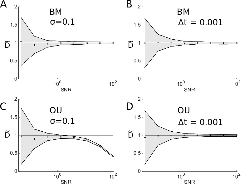
Using formula (20), with 10,000 points, we estimated the diffusion coefficient $\tilde{D}$ in Fig. 1A-B. The signal to noise ratio (SNR) is defined as $\frac{D}{\frac{\sigma^{2}}{\Delta t}}$. We also estimated the diffusion coefficient for an Ornstein-Uhlenbeck process (Fig. 1C-D). These numerical results show that the estimator for the diffusion coefficient is biased for a high SNR, due to the approximation $X_{n+1}-X_{n}\sim\mathcal{N}(a(X_{n})\Delta t,\sqrt{2D\Delta t})$, which is only valid for a small time step $\Delta t$. However this approximation is acceptable for a Brownian motion, as shown in Fig. 1A and 1B.

For a stochastic process containing a drift component, it is not possible to extract the physical diffusion coefficient directly by combining the first and the second moment estimators, which is in contrast with the pure diffusion case (see [13, 14]). We now present an estimator where the Gaussian instrumental noise can be eliminated. Using the difference $\Delta\mbox{\boldmath$Y$}_{n}=\mbox{\boldmath$Y$}_{n+1}-\mbox{\boldmath$Y$}_{n}$, we can rewrite

	$\displaystyle\Delta\mbox{\boldmath$Y$}_{n}$	$\displaystyle=$	$\displaystyle a(\mbox{\boldmath$X$}_{n})\Delta t+{\sigma(\mbox{\boldmath$X$}_{n})}\Delta W_{n}+\sigma(\eta_{n+1}-\eta_{n})$
	$\displaystyle\Delta\mbox{\boldmath$Y$}_{n-1}$	$\displaystyle=$	$\displaystyle a(\mbox{\boldmath$X$}_{n-1})\Delta t+{\sigma(\mbox{\boldmath$X$}_{n-1})}\Delta W_{n-1}+\sigma(\eta_{n}-\eta_{n-1}),$

where $\Delta W_{n}$ and $\Delta W_{n-1}$ are two independent increments of Brownian motion. The expectation is

$\displaystyle E\left[\frac{(Y_{n+1}-Y_{n})(Y_{n}-Y_{n-1})}{\Delta t}\right]=-\frac{\sigma^{2}}{\Delta t}E(\eta^{2}_{n})=-\frac{\sigma^{2}}{\Delta t}+o(1).$

(21)

Using relation (20), we obtain that

$\displaystyle E\left[\frac{(Y_{n+1}-Y_{n})^{2}}{2\Delta t}|Y_{n}=x\right]+E\left[\frac{(Y_{n+1}-Y_{n})(Y_{n}-Y_{n-1})}{\Delta t}\right]=D+\sigma^{2}a^{\prime}(x)+o(1).$

(22)

In this estimator, the instrumental noise is averaged out. However, there are no direct procedures to get rid of the derivative of the drift term, which can be extracted from the first order moment. However, computing a derivative from noisy data should be done carefully as it introduces singularities and irregularities.

We shall now consider an Ornstein-Uhlenbeck process,

$\displaystyle dX=-\lambda(X-\mu)dt+\sqrt{2D}dW,$

(23)

where the pdf is

$\displaystyle p(y,t|x,0)=\frac{1}{\sqrt{2\pi D\frac{(1-e^{-2\lambda t})}{\lambda}}}\exp(-\frac{(y-\mu-(x-\mu)e^{-\lambda t})^{2}}{\frac{2D}{\lambda}(1-e^{-2\lambda t})}).$

(24)

In the discretized setting, the pdf between two time steps separated by an interval $\Delta t$ associated to the observed motion $Y_{n}$, can be computed from eq. () and is given by

	$\displaystyle p(Y_{n+1}=y|Y_{n}=x)$	$\displaystyle=$	$\displaystyle\int\limits_{\mathbb{R}}\int\limits_{\mathbb{R}}\frac{e^{\displaystyle{-}\frac{(y_{1}-\mu-(x_{1}-\mu)e^{-\lambda\Delta t})^{2}}{\frac{2D}{\lambda}(1-e^{-2\lambda\Delta t})}}}{\sqrt{2\pi\frac{D}{\lambda}(1-e^{-2\lambda\Delta t})}}\frac{e^{-\displaystyle{\frac{(x-x_{1})^{2}}{2\sigma^{2}}}}}{\sigma\sqrt{2\pi}}\frac{e^{-\displaystyle{\frac{(y-y_{1})^{2}}{2\sigma^{2}}}}}{\sigma\sqrt{2\pi}}dx_{1}dy_{1}$		(25)
		$\displaystyle=$	$\displaystyle\int\limits_{\mathbb{R}}\frac{e^{-\displaystyle{\frac{(x-x_{1})^{2}}{2\sigma^{2}}}}}{\sigma\sqrt{2\pi}}\frac{e^{-\displaystyle{\frac{(y-\mu-(x_{1}-\mu)e^{-\lambda\Delta t})^{2}}{2(\sigma^{2}+\frac{D}{\lambda}(1-e^{-2\lambda\Delta t}))}}}}{\sqrt{2\pi(\sigma^{2}+\frac{D}{\lambda}(1-e^{-2\lambda\Delta t}))}}dx_{1}$
		$\displaystyle=$	$\displaystyle\frac{e^{-\displaystyle{\frac{(y-\mu-(x-\mu)e^{-\lambda\Delta t})^{2}}{2(\sigma^{2}(1+e^{-2\lambda\Delta t})+\frac{D}{\lambda}(1-e^{-2\lambda\Delta t}))}}}}{\sqrt{2\pi(\sigma^{2}(1+e^{-2\lambda\Delta t})+\frac{D}{\lambda}(1-e^{-2\lambda\Delta t}))}}.$

The local dynamics can be recovered from the trajectories by computing the observed drift at time scale $\Delta t$, which is given by

	$\displaystyle a^{OU}_{\Delta t}(x)$	$\displaystyle=$	$\displaystyle\frac{1}{\Delta t}\int_{\mathbb{R}}(y-x)p(Y_{n+1}=y|Y_{n}=x)dy$		(26)
		$\displaystyle=$	$\displaystyle-(x-\mu)\frac{1-e^{-\lambda\Delta t}}{\Delta t},$

which generalizes relation (18). Similarly, the observed diffusion coefficient is

	$\displaystyle D^{OU}_{\Delta t}(x)$	$\displaystyle=$	$\displaystyle\frac{1}{2\Delta t}\int_{\mathbb{R}}(y-x)^{2}p(Y_{n+1}=y|Y_{n}=x)dy$
		$\displaystyle=$	$\displaystyle\frac{1}{2\Delta t}\left(\sigma^{2}(1+e^{-2\lambda\Delta t})+\frac{D}{\lambda}(1-e^{-2\lambda\Delta t})\right)+(\mu-x)^{2}\frac{(1-e^{-\lambda\Delta t})^{2}}{2\Delta t}.$

In Fig. 2, we estimate the local drift and diffusion coefficient for an OU-process and compare the local estimators for the drift (18) with relation (26). For the diffusion tensor, we compare relations (20) and (). At first order approximation for short time step $\Delta t$, estimators (18)(resp. (20)) gives similar result as (26) (resp. ()).

When a particle is fixed at position $X_{0}$, the sampled trajectories are generated by the noise localization with variance $\sigma$. Computing the first moment shows that the particle is not moving and the second moment is used to extract the variance $\sigma$. The observed dynamics is given by the stochastic equation

$\displaystyle Y_{n}=X_{0}+\sigma\eta_{n},$

where $\eta_{n}$ are i.i.d Gaussian variable of variance 1. The transition probability reduces to

$\displaystyle p(Y_{n+1}=y|Y_{n}=x)=p(Y_{n+1}=y)=\frac{e^{-\displaystyle{\frac{(y-X_{0})^{2}}{2\sigma^{2}}}}}{\sigma\sqrt{2\pi}}.$

and the empirical estimator of the drift is

	$\displaystyle a_{\Delta t}(x)$	$\displaystyle=$	$\displaystyle\frac{1}{\Delta t}\int_{\mathbb{R}}(y-x)p(Y_{n+1}=y|Y_{n}=x)dy$
		$\displaystyle=$	$\displaystyle\frac{1}{\Delta t}\int_{\mathbb{R}}(y-x)\frac{e^{-\displaystyle{\frac{(y-X_{0})^{2}}{2\sigma^{2}}}}}{\sigma\sqrt{2\pi}}dy$
		$\displaystyle=$	$\displaystyle-\frac{1}{\Delta t}(x-X_{0}),$

which should be compared to relation (18): the estimator now depends on the time resolution $\Delta t$ and the location of the pinned particles, which can be determined by the empirical averaging $\frac{1}{n}\sum_{k=1}^{n}Y_{k}$. The sum is converging (in probability) as $n$ goes to infinity to the mean $\hbox{\bb E}(Y_{1})=X_{0}$. Thus contrary to the case of a physical drift, the empirical sum $\frac{1}{N}\sum_{k}^{N}\left[\frac{Y^{k}_{n+1}-x}{\Delta t}\right]$ converges $-\frac{1}{\Delta t}(x-X_{0})$, which depends on the time step $\Delta t$.

Similarly the second moment estimator gives for the diffusion coefficient the following expression

	$\displaystyle D_{\Delta t}(x)$	$\displaystyle=$	$\displaystyle E\left[\frac{(Y_{n+1}-Y_{n})^{2}}{2\Delta t}|Y_{n}=x\right]=\frac{1}{2\Delta t}\int_{\mathbb{R}}(y-x)^{2}\frac{e^{-\displaystyle{\frac{(y-X_{0})^{2}}{2\sigma^{2}}}}}{\sigma\sqrt{2\pi}}dy$		(28)
		$\displaystyle=$	$\displaystyle\frac{1}{2\Delta t}((x-X_{0})^{2}+\sigma^{2}).$

By fixing the center $x=X_{0}$, the empirical estimator (28) allows estimating $\frac{1}{2\Delta t}\sigma^{2}$ and the variance $\sigma$.
This example is instructive because it allows differentiating a fixed particle from one trapped in a potential well (see paragraph below). In summary, the following criteria can be used: the first moment (velocity) computed from a sample trajectory for a fixed particle depends on the time resolution $\Delta t$, which is not the case for a physical particle trapped in a potential well (see relation (18)).

To estimate the apparent drift and diffusion tensor, we apply analytical expressions for the pdf (formula 31). Using the formula to characterize the drift at resolution $\Delta t$ [16] at position $x$, we get

	$\displaystyle\mbox{\boldmath$a$}_{\Delta t}(\mbox{\boldmath$x$})$	$\displaystyle=$	$\displaystyle\hbox{\bb E}\left[\frac{\mbox{\boldmath$Y$}_{n+1}-\mbox{\boldmath$Y$}_{n}}{\Delta t}|\mbox{\boldmath$Y$}_{n}=\mbox{\boldmath$x$}\right]$
		$\displaystyle=$	$\displaystyle\frac{1}{\Delta t}\int\limits_{\mathbb{R}^{m}}(\mbox{\boldmath$y$}-\mbox{\boldmath$x$})p(\mbox{\boldmath$Y$}_{n+1}=\mbox{\boldmath$y$}|\mbox{\boldmath$Y$}_{n}=\mbox{\boldmath$x$})d\mbox{\boldmath$y$}$
		$\displaystyle=$	$\displaystyle\frac{1}{(2\pi)^{m/2}\Delta t}\int\limits_{\mathbb{R}^{m}}\frac{(\mbox{\boldmath$y$}-\mbox{\boldmath$x$})d\mbox{\boldmath$y$}}{\sqrt{\det\mbox{\boldmath$\Sigma$}(\mbox{\boldmath$x$})}}e^{\displaystyle{-\frac{1}{2}(\mbox{\boldmath$y$}-\Delta t\mbox{\boldmath$A$}(\mbox{\boldmath$x$})-\mbox{\boldmath$x$})^{T}\mbox{\boldmath$\Sigma$}^{-1}(\mbox{\boldmath$x$})(\mbox{\boldmath$y$}-\Delta t\mbox{\boldmath$A$}(\mbox{\boldmath$x$})-\mbox{\boldmath$x$})}}.$

Using the change of variable $\mbox{\boldmath$v$}=\mbox{\boldmath$y$}-\Delta t\mbox{\boldmath$A$}(\mbox{\boldmath$x$})-\mbox{\boldmath$x$}$ we obtain

	$\displaystyle\mbox{\boldmath$a$}_{\Delta t}(\mbox{\boldmath$x$})$	$\displaystyle=$	$\displaystyle\frac{1}{\Delta t}\int\limits_{\mathbb{R}^{m}}(\mbox{\boldmath$v$}+\Delta t\mbox{\boldmath$A$}(\mbox{\boldmath$x$}))\frac{1}{\sqrt{(2\pi)^{m}\det\mbox{\boldmath$\Sigma$}(\mbox{\boldmath$x$})}}e^{\displaystyle{-\frac{1}{2}\mbox{\boldmath$v$}^{T}\mbox{\boldmath$\Sigma$}^{-1}(\mbox{\boldmath$x$})\mbox{\boldmath$v$}}}d\mbox{\boldmath$v$}$		(33)
		$\displaystyle=$	$\displaystyle\mbox{\boldmath$A$}(\mbox{\boldmath$x$})+o(\Delta t).$

This approximation is valid to second order in $\sigma$ (see Appendix B). Similarly in the isotropic case, the diffusion coefficient at position $x$ can be recovered from the second order moment approximation

$\displaystyle D_{\Delta t}(\mbox{\boldmath$x$})$

$\displaystyle=$

$\displaystyle E\left[\frac{\left\lVert\mbox{\boldmath$Y$}_{n+1}-\mbox{\boldmath$Y$}_{n}\right\rVert^{2}}{2m\Delta t}|\mbox{\boldmath$Y$}_{n}=\mbox{\boldmath$x$}\right].$

(34)

Thus, using the pdf formula (31), we get

	$\displaystyle D_{\Delta t}(\mbox{\boldmath$x$})$	$\displaystyle=$	$\displaystyle\frac{1}{2m\Delta t}\int\limits_{\mathbb{R}^{m}}(\mbox{\boldmath$v$}+\Delta t\mbox{\boldmath$A$}(\mbox{\boldmath$x$}))^{T}(\mbox{\boldmath$v$}+\Delta t\mbox{\boldmath$A$}(\mbox{\boldmath$x$}))\frac{1}{\sqrt{(2\pi)^{m}\det\mbox{\boldmath$\Sigma$}(\mbox{\boldmath$x$})}}e^{\displaystyle{-\frac{1}{2}\mbox{\boldmath$v$}^{T}\mbox{\boldmath$\Sigma$}(\mbox{\boldmath$x$})^{-1}\mbox{\boldmath$v$}}}d\mbox{\boldmath$v$}$		(35)
		$\displaystyle=$	$\displaystyle\frac{1}{2m\Delta t}\int\limits_{\mathbb{R}^{m}}(\mbox{\boldmath$v$}^{T}\mbox{\boldmath$v$}+\Delta t(\mbox{\boldmath$A$}(\mbox{\boldmath$x$})^{T}+\mbox{\boldmath$A$}(\mbox{\boldmath$x$}))+\Delta t^{2}\mbox{\boldmath$A$}(\mbox{\boldmath$x$})^{T}\mbox{\boldmath$A$}(\mbox{\boldmath$x$}))\times$
			$\displaystyle\frac{1}{\sqrt{(2\pi)^{m}\det\mbox{\boldmath$\Sigma$}(\mbox{\boldmath$x$})}}e^{\displaystyle{-\frac{1}{2}\mbox{\boldmath$v$}^{T}\mbox{\boldmath$\Sigma$}(\mbox{\boldmath$x$})^{-1}\mbox{\boldmath$v$}}}d\mbox{\boldmath$v$}$
		$\displaystyle=$	$\displaystyle\frac{1}{2m\Delta t}(Tr(\mbox{\boldmath$\Sigma$}(\mbox{\boldmath$x$}))+O(\Delta t^{2})).$

Using eq. (31), we have

$\displaystyle Tr(\mbox{\boldmath$\Sigma$}(\mbox{\boldmath$x$}))=m(2\sigma^{2}+2D\Delta t)+2\sigma^{2}\Delta tTr(\mbox{\boldmath$J$}(\mbox{\boldmath$x$}))+O(\Delta t^{2}).$

(36)

Finally,

$\displaystyle D_{\Delta t}(\mbox{\boldmath$x$})=D+\frac{\sigma^{2}}{\Delta t}+\frac{\sigma^{2}}{m}div(\mbox{\boldmath$A$})+O(\Delta t),$

(37)

where by definition, in local coordinates $div(\mbox{\boldmath$A$})=\displaystyle{\sum}_{i=1}^{m}\frac{\partial a_{i}(\mbox{\boldmath$x$})}{\partial x_{i}}$. In general, the diffusion tensor can be approximated at order $\Delta t$ by

	$\displaystyle D^{ij}_{\Delta t}(\mbox{\boldmath$x$})$	$\displaystyle=$	$\displaystyle E\left[\frac{(\mbox{\boldmath$Y$}_{n+1}-\mbox{\boldmath$Y$}_{n})^{i}(\mbox{\boldmath$Y$}_{n+1}-\mbox{\boldmath$Y$}_{n})^{j}}{2\Delta t}|\mbox{\boldmath$Y$}_{n}=\mbox{\boldmath$x$}\right]$		(38)
		$\displaystyle=$	$\displaystyle\frac{1}{2\Delta t}\int\limits_{\mathbb{R}^{m}}(\mbox{\boldmath$v$}+\Delta t\mbox{\boldmath$A$}(\mbox{\boldmath$x$}))^{i}(\mbox{\boldmath$v$}+\Delta t\mbox{\boldmath$A$}(\mbox{\boldmath$x$}))^{j}\frac{1}{\sqrt{(2\pi)^{m}\det\mbox{\boldmath$\Sigma$}(\mbox{\boldmath$x$})}}e^{\displaystyle{-\frac{1}{2}\mbox{\boldmath$v$}^{T}\mbox{\boldmath$\Sigma$}(\mbox{\boldmath$x$})^{-1}\mbox{\boldmath$v$}}}d\mbox{\boldmath$v$}$
		$\displaystyle=$	$\displaystyle D^{ij}+\frac{\sigma^{2}}{\Delta t}\delta_{ij}+\frac{\sigma^{2}}{2}(\mbox{\boldmath$J$}(\mbox{\boldmath$x$})+\mbox{\boldmath$J$}^{T}(\mbox{\boldmath$x$}))^{ij}+O(\Delta t).$

References

• [1] Hoze N., Nair D, Hosy E, Sieben C, Manley S, Herrmann A, Sibarita JB, Choquet D, Holcman D. Heterogeneity of AMPA receptor trafficking and molecular interactions revealed by superresolution analysis of live cell imaging. Proc Natl Acad Sci U S A. 2012;109(42):17052-7. 2012.
• [2] Hoze, N., D. Holcman, Residence times of receptors in dendritic spines analyzed by stochastic simulations in empirical domains, Biophys J. 2014;107(12):3008-17.
• [3] Saxton, M.J. and K. Jacobson (1997), Single-particle tracking: applications to membrane dynamics, Annu. Rev. Biophys. Biomol. Struct. 26, pp.373–399.
• [4] Saxton M.J., Single-particle tracking: connecting the dots.Nat Methods. 2008 Aug;5(8):671-2.
• [5] D. Arcizet, B. Meier, E. Sackmann, J. O. Rädler, and D. Heinrich, Temporal analysis of active and passive transport in living cells. Phys. Rev. Lett. 101, 248103 (2008).
• [6] Nandi A, Heinrich D, Lindner B, Distributions of diffusion measures from a local mean-square displacement analysis. Phys Rev E Stat Nonlin Soft Matter Phys. 2012;86:021926.
• [7] Kusumi, A., Y. Sako and M. Yamamoto (1993),Confined lateral diffusion of membrane receptors as studied by single particle tracking (nanovid microscopy). Effects of calcium-induced differentiation in cultured epithelial cells, Biophys J. 65, pp.2021–2040.
• [8] Holcman D., Unraveling novel features hidden in superresolution microscopy data. Commun Integr Biol. 2013 1;6(3):e23893.
• [9] Holcman D, Hoze N, Schuss Z. Narrow escape through a funnel and effective diffusion on a crowded membrane, Phys Rev E 2011, 84(2-1):021906.
• [10] B. Meier, A. Zielinski, C. Weber, D. Arcizet, S. Youssef, T. Franosch, J. O. Rädler, and D. Heinrich, Chemotactic cell trapping in controlled alternating gradient fields, Proc. Natl. Acad. Sci. 108(28):11417-11422 (2011).
• [11] D. Arcizet, S. Capito, M. Gorelashvili, C. Leonhard, M. Vollmer, S. Youssef, S. Rappl and D. Heinrich, Contact-controlled amoeboid motility induces dynamic cell trapping in 3D-microstructured surfaces. Soft Matter 8(5):1473-1481 (2012)
• [12] M. Gorelashvili, M. Emmert, K. Hodeck and D. Heinrich, Amoeboid migration mode adaption in quasi-3D spatial density gradients of varying lattice geometry, New J. Phys. 16, 075012 (2014)
• [13] A. J. Berglund, Statistics of camera-based single-particle tracking, Phys. Rev. E 82, 011917 (2010).
• [14] Verstergaard, C.L., P. Blainey and H. Flyvbjerg (2014), Optimal estimation of diffusion coefficients from single-particle trajectories.Phys. Rev. E, 89, 022726.
• [15] R.E. Thompson, D.R. Larson, and W.W. Webb, Precise nanometer localization analysis for individual fluorescent probes. Biophys J. 2002; 82(5): 2775–2783.
• [16] Schuss, Z. (2012) Nonlinear Filtering and Optimal Phase Tracking, Springer series on Applied Mathematical Sciences vol.180, Springer NY.
• [17] Schuss, Z. (1980), Theory and Applications of Stochastic Differential Equations. Wiley Series in Probability and Statistics. John Wiley Sons, Inc., New York.
• [18] Schuss, Z. (2010) Diffusion and Stochastic Processes: an Analytical Approach. Springer series on Applied Mathematical Sciences vol.170, Springer NY.
• [19] S. Karlin and H.M. Taylor. A second course in stochastic processes. Academic Pr, 1981.
• [20] Manley, S., J.M. Gillette, G.H. Patterson, H. Shroff, H.F. Hess, E. Betzig, and J. Lippincott-Schwartz (2008), High-density mapping of single-molecule trajectories with photoactivated localization microscopy. Nature Methods 5, pp.155–157.