Time-optimal polarization transfer from an electron spin to a nuclear spin

As the gyromagnetic ratio of an electron is two to three orders of magnitude larger than the one of a nucleus, electron spins are much easier polarized than nuclear spins. This offers a way to improve the polarization of nuclear spins by transferring polarization from electron spins to nuclear spins; much higher nuclear spin polarization can be achieved as compared to a direct polarization. This idea has been widely used in various physical settings, for example dynamic nuclear polarization (DNP) [1, 2, 3, 4, 5, 6] employs this idea to dramatically improve the sensitivity of nuclear magnetic resonance (NMR) [7, 8]. It is also frequently used on various hybrid electron-nuclear spin systems, such as organic single crystals [9], endohedral fullerenes [10, 11, 12], phosphorous donors in silicon crystals [13], and nitrogen-vacancy centers in diamond [14, 15, 16, 17]. For example, in the case of nitrogen-vacancy centers in diamond, efficient polarization transfers are used to initialize the quantum state of nuclear spins for quantum information processing.

Efficient polarization transfers are practically achieved by properly engineered pulse sequences whose design is studied in the field of quantum control [18, 19, 20, 21, 22, 23]. In recent years, significant progress has been made in quantum control for both numerical [24, 25, 26, 27, 28, 29, 30, 31, 32, 33, 34, 35, 36, 37] and analytical [38, 39, 40, 41] methods. Extensive knowledge has been gained on optimal pulse sequences for two- and three-level systems [42, 43, 44, 45, 46, 47, 48, 49, 50, 51, 52, 53, 54, 55, 56], two uncoupled spins [57, 58], and two coupled spins [59, 60, 61, 62, 63, 64, 65]. Further advances have been made on how to optimally control multiple coupled spins [66, 67, 68, 69, 70, 71, 72, 73, 74, 75, 76, 77, 78, 79, 80, 81, 82, 83, 84, 85, 86, 87, 88, 89, 90, 91]. These methods have been successfully applied in NMR [92, 93] to designing broad-band [94, 95, 96] and decoupling pulse sequences [97, 98, 99, 100, 101, 102]. They have also been utilized in magnetic resonance imaging [25, 103, 104, 105] and electron paramagnetic resonance [106].

In this article, we consider time-optimal pulse sequences for polarization transfers from an electron spin to a nuclear spin. Relaxation and decoherence are in practice inevitable and result in a loss of signal. But their effect can be mitigated by short pulse sequences which allow for highly sensitive experiments. We analyze and explain how the form of time-optimal sequences depends on the direction of the polarization by studying time-optimal transfers for different directions.

Recent analytical [107] and numerical [108, 109] studies focused on low-field single-crystal experiments, where the nuclear Larmor frequency and pseudo-secular hyperfine interaction (see Sect. 3.5 of Ref. [1]) are comparable in magnitude. As in [110, 111, 112, 113], we focus here on the cases of secular hyperfine coupling (see Sect. 3.5 of Ref. [1]). These assumptions are satisfied in liquid-state and high-field solid-state DNP.

We analyze two particular cases of polarization transfers and determine the corresponding time-optimal sequences. In Section II, we consider the transfer from the state $S_{z}$ of the electron spin to the state $I_{z}$ of the nuclear spin. The second time-optimal transfer from $S_{z}$ to $I_{x}$ is presented in Section III. And most interestingly, the corresponding optimal transfer time is shorter by $78.5\%$ when compared to the transfer from $S_{z}$ to $I_{z}$, which highlights that the transfer efficiency depends crucially on the target state of the nuclear spin. We discuss our results in Section IV, and the possibility of a non-sinusoidal carrier wave form is entertained in Section V. We conclude in Section VI, and certain details are relegated to Appendices A and B.

In this section, we study the polarization transfer from the initial state $S_{z}$ to the final state $I_{z}$ ¹¹ 1 Note that we only consider the (rescaled) traceless part $\rho$ of the actual density matrix $b\rho+\frac{1}{4}I$, where $b$ denotes the Boltzmann factor. As the identity component does not evolve, it can be neglected.. We assume a secular hyperfine coupling (see Sect. 3.5 of Ref. [1]). In the lab frame, the resulting Hamiltonian is given by

where $\omega_{S}$ and $\omega_{I}$ denote the respective Larmor frequencies of the electron and the nuclear spin, $A$ represents the strength of the secular hyperfine coupling, $\tilde{u}_{x}(t)$ and $\tilde{v}_{x}(t)$ are the amplitudes of the control fields. Here, $S_{j}=(\sigma_{j}\otimes\sigma_{0})/2$ acts on the electron spin and $I_{k}=(\sigma_{0}\otimes\sigma_{k})/2$ acts on the nuclear spin with $j,k\in\{x,y,z\}$, where $\sigma_{0}:=\left(\begin{smallmatrix}1&0\\ 0&1\end{smallmatrix}\right)$ denotes the identity matrix and the Pauli matrices are $\sigma_{x}:=\left(\begin{smallmatrix}0&1\\ 1&0\end{smallmatrix}\right)$, $\sigma_{y}:=\left(\begin{smallmatrix}0&-i\\ i&\phantom{-}0\end{smallmatrix}\right)$, and $\sigma_{z}:=\left(\begin{smallmatrix}1&\phantom{-}0\\ 0&-1\end{smallmatrix}\right)$. For typical NMR settings, only a single radio-frequency coil is used which can be assumed to be oriented along the $x$ axis of the lab frame. Hence, only a single control $\tilde{v}_{x}(t)$ appears for the nuclear spin in the lab frame Hamiltonian of Eq. (1). We assume in this work that the carrier wave form for the nuclear spin has a sinusoidal shape, i.e. $\tilde{v}_{x}(t)=v(t)\cos[\omega_{I}^{\mathrm{rf}}t+\phi(t)]$ with amplitude $v(t)\leq 2v_{\mathrm{max}}$ and phase $\phi_{0}$. Here, $\omega_{I}^{\mathrm{rf}}$ is the carrier frequency of the radio-frequency irradiation and $2v_{\mathrm{max}}$ denotes the maximal control amplitude (in the lab frame). This choice of $\tilde{v}_{x}(t)$ is motivated by the properties (e.g., bandwidth limitations) of the usually available wave form generators and amplifiers. More general carrier wave forms are discussed in Section V.

By switching to the rotating frame of $\omega_{S}S_{z}+\omega_{I}^{\mathrm{rf}}I_{z}$ corresponding to the carrier frequencies $\omega_{S}$ and $\omega_{I}^{\mathrm{rf}}=\omega_{I}-\omega_{I}^{\mathrm{off}}$ and applying the rotating wave approximation, we get an effective Hamiltonian

One can obtain any desired offset term $\omega_{I}^{\mathrm{off}}I_{z}$ in the drift term of $H_{\mathrm{rot}}$ in Eq. (2) by suitably choosing the carrier frequency $\omega_{I}^{\mathrm{rf}}$ ²² 2 In [110], the choice for $\omega_{I}^{\mathrm{off}}$ was $\omega_{I}^{\mathrm{off}}=\pi A$.. For simplicity, $\omega_{I}^{\mathrm{off}}$ is set to zero in the following. The microwave-frequency control pulses on the electron spin and the radio-frequency control pulses on the nuclear spin are given by $H^{\mathrm{mw}}_{\mathrm{rot}}$ and $H^{\mathrm{rf}}_{\mathrm{rot}}$, respectively. The control amplitudes $u_{x}(t)$, $u_{y}(t)$, $v_{x}(t)$, and $v_{y}(t)$ satisfy the bounds

where $u_{\mathrm{max}}$ and $v_{\mathrm{max}}$ denote the maximal available amplitudes of the control fields in the rotating frame for a given experiment. This is a result of the rotating wave approximation, which reduces the maximal control amplitude of $2v_{\mathrm{max}}$ in lab frame to $v_{\mathrm{max}}$ in the rotating frame [8]. In the following, we will assume that $u_{\mathrm{max}}\gg A\gg v_{\mathrm{max}}$ and neglect the time needed to apply operations that can be generated by the hyperfine coupling and the controls on the electron spin ³³ 3 Strictly speaking, our results are also applicable when only the conditions $A\gg v_{\mathrm{max}}$ and $u_{\mathrm{max}}\gg v_{\mathrm{max}}$ are fulfilled..

Time-optimal transformations are essentially only limited by the weak controls on the nuclear spin. The optimal strategy to achieve a desired transfer can be inferred from the structure of cosets with respect to the fast operations [59, 66, 110]. Here, the fast operations are given by the hyperfine coupling and the strong controls on the electron spin. The transformation $U$ which transfers $S_{z}$ to $I_{z}=US_{z}U^{-1}$ will be suitably decomposed into a product $U=U_{2}U_{1}$. The unitary $U_{1}$ transfers the initial state $S_{z}$ to the intermediate state $2S_{z}I_{z}=U_{1}S_{z}U_{1}^{-1}$, and it can be generated using only fast operations. In addition, the unitary $U_{2}$ transfers the intermediate state $2S_{z}I_{z}$ to the final state $I_{z}=U_{2}(2S_{z}I_{z})U_{2}^{-1}$, and one has to use the weak controls on the nuclear spin in order to generate $U_{2}$. Below, we will provide a time-optimal scheme to produce $U_{2}$. This results also in a time-optimal scheme for $U$ as any faster scheme for $U$ would also imply a faster one for $U_{2}=UU_{1}^{-1}$.

The polarization transfer from $S_{z}$ to $I_{z}$ can be decomposed into the following steps ⁴⁴ 4 The notation $A\xrightarrow{B}C$ describes that polarization is transferred from $A$ to $C$ by applying the unitary transfer $C=\exp(-iB)A\exp(iB)$.:

where we denote

then $\pi S^{\beta}I_{y}=-\pi S_{z}I_{y}+\pi I_{y}/2$. As shown in Eq. (3), the polarization transfer from $S_{z}$ to $2S_{z}I_{z}$ is accomplished using an INEPT-type transfer [118, 8]: First, we apply a hard ${\pi}/{2}$ pulse to the electron spin along the $+y$ direction (i.e. $S_{y}$). Then, we let the hyperfine coupling evolve for the duration of $1/(2A)$ units of time. Another hard ${\pi}/{2}$ pulse on the electron spin along the $+x$ direction completes the transfer to $2S_{z}I_{z}$. All of these steps take negligible time, since they are either local operations on the electron spin or operations which can be generated by the coupling. In conclusion, we can completely focus on the last step in Eq. (3) where we need to generate the propagator

for $\theta=\pi$. The operator in the exponent of $U^{\beta}_{y}(\theta)$ in Eq. (4) is a single-transition operator [8, 1]. In particular, the operator $U^{\beta}_{y}(\pi)=\exp(-i\pi S^{\beta}I_{y})$ describes a transition-selective $\pi$ rotation around the $y$ axis in the subspace spanned by the basis states $|\beta\alpha\rangle{}$ and $|\beta\beta\rangle{}$, where the subspace corresponds to the $\beta$ component of the nuclear spin doublet at frequency $\omega_{I}/(2\pi)+A/2$ [119] as shown in Figures 1 and 2. Here, $|\alpha\rangle{}$ and $|\beta\rangle{}$ are eigenstates of $S_{z}$ and $I_{z}$, e.g., $S_{z}|\alpha\rangle{}=|\alpha\rangle{}/2$ and $S_{z}|\beta\rangle{}=-|\beta\rangle{}/2$.

In the following, we determine a time-optimal scheme to produce the unitary $U^{\beta}_{y}(\pi)$. The set of all unitaries which transfer $2S_{z}I_{z}$ to $I_{z}$ are discussed in Appendix A.1, where we also show by extending the results in the current section that choosing a different element from this set of unitaries does not lead to a shorter transfer time.

To determine the optimal transfer, we switch to the interacting frame of $2\pi AS_{z}I_{z}$ by applying the transformation $\exp(i2\pi AS_{z}I_{z}t)H_{\mathrm{rot}}\exp(-i2\pi AS_{z}I_{z}t)$. The Hamiltonian of Eq. (2) changes to ⁵⁵ 5 In the interaction frame, $H_{\mathrm{rot}}$ is transformed into $H_{\mathrm{int}}=\exp(i2\pi AS_{z}I_{z}t)H_{\mathrm{rot}}\exp(-i2\pi AS_{z}I_{z}t)-2\pi AS_{z}I_{z}$.

where $S^{\alpha}I_{y}=S_{z}I_{y}+I_{y}/2$ and $S^{\beta}I_{y}=-S_{z}I_{y}+I_{y}/2$.

We aim at generating the operator $U_{y}^{\beta}(\pi)$ in minimum time, which corresponds to maximizing the coefficient $2\pi[v_{x}(t)\sin({\pi At})+v_{y}(t)\cos(\pi At)]$ in front of $S^{\beta}I_{y}$. The Cauchy-Schwarz inequality implies

where the second inequality is a consequence of the constraints on the amplitude of the control fields. The maximal value of $2\pi[v_{x}(t)\sin({\pi At})+v_{y}(t)\cos(\pi At)]$ is denoted by $2\pi v_{\mathrm{max}}$ and it can be achieved by choosing the controls $u_{x}(t)=u_{y}(t)=0$, $v_{x}(t)=v_{\mathrm{max}}\sin(\pi At)$, $v_{y}(t)=v_{\mathrm{max}}\cos(\pi At)$. To understand that this choice generates the desired operator, one can substitute the controls in the Hamiltonian with the chosen values and obtains

Since $A\gg v_{\mathrm{max}}$, average Hamiltonian theory implies that the first three terms average out to zero; and one is left with the desired Hamiltonian $2\pi v_{\mathrm{max}}S^{\beta}I_{y}$.

The minimum time to generate $U^{\beta}_{y}(\pi)$ is then fixed by the relation $2\pi v_{\mathrm{max}}T_{\mathrm{min}}=\pi$, and one obtains

The presented time-optimal control corresponds to a radio-frequency irradiation at frequency $\omega_{I}/(2\pi)+A/2$ with duration $T_{\mathrm{min}}$, which results in a transition-selective inversion of the $\beta$ line of the nuclear spin doublet. This belongs to the class of controls presented in Ref. [110] and is also closely related to selective population inversion (SPI) experiments [121, 122, 123, 124].

We can also compute the maximal transfer efficiency $\eta_{max}(T)$ for a given time $T$. The operator $U^{\beta}_{y}(\theta)$ transfers the state $2S_{z}I_{z}$ to the state

For $\theta=2\pi v_{\mathrm{max}}T$, we get the maximal transfer efficiency

for the transfer to $I_{z}$. Note that $\eta_{max}(T_{\mathrm{min}})=1$.

We compare our analytic results with numerical optimizations for achieving the transfer from $S_{z}$ to $I_{z}$ as shown in Fig. 3, cf. [111, 112, 113]. For these optimizations, the hyperfine coupling constant is chosen as $A=10\text{ MHz}$ and the maximal allowed radiation amplitudes are set to $u_{\mathrm{max}}=1\text{ MHz}$ and $v_{\mathrm{max}}=20\text{ kHz}$ ⁶⁶ 6 Even though we have $u_{\mathrm{max}}<A$, the crucial requirements $A\gg v_{\mathrm{max}}$ and $u_{\mathrm{max}}\gg v_{\mathrm{max}}$ for optimality are fulfilled.. In Fig. 3, the transfer is completed after $25\mu s=1/(2v_{\mathrm{max}})$ units of time which agrees with the analytically computed time. Moreover, the form of the numerically optimized controls compares nicely with the analytic results: the values of $u_{x}(t)$ and $u_{y}(t)$ are most of the time small (except for the beginning), and $v_{x}(t)$ and $v_{y}(t)$ have a sinusoidal form with the maximal allowed amplitude.

We analyze now how to time-optimally transfer polarization from the state $S_{z}$ to $I_{x}$ (and similarly for the transfer to $I_{y}$). The considered transfer consists of the following steps:

where $\tfrac{\pi}{2}S^{\alpha}I_{y}-\tfrac{\pi}{2}S^{\beta}I_{y}=\pi S_{z}I_{y}$. As in Sec. II, we can focus on generating the final propagator $\tilde{U}_{2}=\exp(-i\pi S_{z}I_{y})$ in the product $\tilde{U}=\tilde{U}_{2}U_{1}$. The transfer $I_{x}=\tilde{U}S_{z}\tilde{U}^{-1}$ is decomposed into a fast transfer to the intermediate state $2S_{z}I_{z}=U_{1}S_{z}U_{1}^{-1}$ and a slow transfer to final state $I_{x}=\tilde{U}_{2}(2S_{z}I_{z})\tilde{U}_{2}^{-1}$. Building on the results in this section, we prove in Appendix A.2 that one cannot reduce the transfer time by substituting $\tilde{U}_{2}$ with a different unitary $V$ satisfying $I_{x}=V(2S_{z}I_{z})V^{-1}$.

Previously, the propagator $\exp(-i\pi S_{z}I_{y})$ in the final step has been achieved [110] by applying a transition-selective radio-frequency $-\pi/2$ pulse along the $y$ direction at the $\beta$ transition with frequency $\omega_{I}/(2\pi)+A/2$ as well as a transition-selective radio-frequency $\pi/2$ pulse along the $y$ direction at the $\alpha$ transition with frequency $\omega_{I}/(2\pi)-A/2$, see Fig. 4. In the rotating frame of Eq. (2), this irradiation scheme on the nuclear spin corresponds to a radio-frequency Hamiltonian of the form

Note that in this scheme the $\alpha$ and $\beta$ transitions can only be irradiated with a radio-frequency amplitude of $v_{\mathrm{max}}/2$ in order not to exceed the maximal available radio-frequency amplitude $v_{\mathrm{max}}$ for the overall irradiation at the nuclear spin. Hence, the duration for the simultaneous $\pm\pi/2$ pulses along the $y$ direction at the $\alpha$ and $\beta$ transitions is equal to $1/(2v_{\mathrm{max}})$. This conventional transfer is optimal if one considers only pulses at the frequencies $\omega_{I}/(2\pi)\pm A/2$ of the nuclear-spin doublet (refer to [110] and the discussion in Section IV).

Here, we show that shorter pulses are possible if one considers more general transfer schemes. Without exceeding $v_{\mathrm{max}}$, shorter pulses can be obtained by irradiating at the frequencies $\omega_{I}/(2\pi)\pm A/2$ with higher intensity since the resulting higher amplitude can be then decreased by irradiating at additional well selected frequencies. Our approach is quite effective although it might seem counterintuitive at first.

In the interaction frame of $2\pi AS_{z}I_{z}$, the Hamiltonian is again given by Eq. (5). In order to generate the operator $\exp(-i\pi S_{z}I_{y})$ in minimum time, we maximize the coefficient $-2\pi v_{x}(t)\sin(\pi At)$ of $2S_{z}I_{y}$. Note that

where the second equality is implied by the constraint $|v_{x}(t)|\leq\sqrt{v_{x}^{2}(t)+v^{2}_{y}(t)}\leq v_{\mathrm{max}}$ on the control amplitudes. Therefore, the maximal value $2\pi v_{\mathrm{max}}|\sin(\pi At)|$ for $-2\pi v_{x}(t)\sin(\pi At)$ can be attained by choosing the controls $u_{x}(t)=u_{y}(t)=v_{y}(t)=0$ and $v_{x}(t)=-\mathrm{sgn}[\sin(\pi At)]v_{\mathrm{max}}$. This means that $v_{x}(t)$ is a square wave such that $v_{x}(t)=v_{\mathrm{max}}$ when $\sin(\pi At)<0$ and $v_{x}(t)=-v_{\mathrm{max}}$ when $\sin(\pi At)>0$. In this case, the radio-frequency Hamiltonian in the rotating frame is given by

We obtain the minimum time

for generating $\exp(-i\pi S_{z}I_{y})$ in the interaction frame. The duration of the transfer is reduced to $78.5\%$ of the length of the conventional pulse sequence. By transforming the operator back to the rotating frame, we obtain the operator $\exp(-i\phi S_{z}I_{z})\exp(-i\pi S_{z}I_{y})\exp(i\phi S_{z}I_{z})$ where $\phi=2\pi AT_{\mathrm{min}}$ denotes the phase accumulated during the time $T_{\mathrm{min}}=\pi/(8v_{\mathrm{max}})$. The effect of this superfluous phase $\phi$ can be reversed using the hyperfine coupling $2\pi AS_{z}I_{z}$ which takes only a negligible time period as the coupling strength $A$ is much larger than the control strength $v_{\mathrm{max}}$ of the nuclear spin. Thus, the minimum time in the rotating frame is also given by $\pi/(8v_{\mathrm{max}})$. Similarly as in Eq. (7), we compute the maximal transfer efficiency

that can be reached for the polarization transfer from $S_{z}$ to $I_{x}$ in a specified time $T$.

Transferring the state from $S_{z}$ to $I_{y}$ is similar. We set $u_{x}(t)=u_{y}(t)=v_{x}(t)=0$ and maximize the coefficient $-2\pi v_{y}(t)\sin(\pi At)$ of $-2S_{z}I_{x}$ in Eq. (5) by setting $v_{y}(t)=-\mathrm{sgn}[\sin(\pi At)]v_{\mathrm{max}}$. The minimum time for this case is also given by $\pi/(8v_{\mathrm{max}})$.

A numerically optimized pulse sequence for transferring polarization from $S_{z}$ to $I_{x}$ is shown in Fig. 5, cf. [111, 112, 113]. The maximal transfer efficiency is reached after $20\mu s$ which is consistent with the analytical result of $\pi/(8v_{\mathrm{max}})\approx 19.635\mu s$.

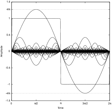
We see that the minimum time for transferring $S_{z}$ to $I_{x}$ or $I_{y}$ is shorter by a factor of $\pi/4$ when compared to the minimum time for transferring $S_{z}$ to $I_{z}$. This factor can be explained by a closer examination of the pulse sequences. The radio-frequency sequence for the transfer from $S_{z}$ to $I_{z}$ shows a sine-cosine wave modulation of maximal amplitude for the $v_{x}$- and $v_{y}$-components (see Fig. 3). However, the radio-frequency sequence for the transfer from $S_{z}$ to $I_{x}$ consists of a square wave of maximal amplitude for the $v_{x}$-component of the control (see Fig. 5). The higher effective amplitude at the two frequencies $\omega_{I}/(2\pi)\pm A/2$ and the shorter transfer time can be explained by decomposing the square wave into a sum of sine waves:

This is illustrated in Fig. 6 where the first sine wave function has an amplitude which is larger by a factor of $4/\pi$ when compared to the amplitude of the square wave. Therefore, the square wave contains implicitly a sine wave with an higher effective amplitude. This implies that the duration of the simultaneous $\pm\pi/2$ rotations of the $\alpha$ and $\beta$ components of the nuclear spin doublet (see Fig. 4) is shorter by a factor of $\pi/4$.

The square-modulated transfer sequence is optimal but needs infinite bandwidth. We also studied numerically how the maximal transfer efficiency varies as a function of time and bandwidth limitations. The results are shown in Fig. 7, cf. [111, 112, 113]. In the case of infinite bandwidth, the results are consistent with the analytical results. The transfer functions $\sin^{2}(\pi v_{\mathrm{max}}t)$ and $\sin(4v_{\mathrm{max}}t)$ for the respective transfers from $S_{z}$ to $I_{z}$ and $I_{x}$ have been obtained in Eqs. (8) and (10).

We compare our results to the time-optimal synthesis of unitary transformations in [110]. Motivated by energy considerations, only irradiations at the two resonance frequencies $\omega_{I}/(2\pi)\pm A/2$ of the control system were considered in [110]. This did not allow for the faster scheme obtained in Section III which has been also observed numerically in [111, 112, 113]. The numerical results in Fig. 7 also show that the faster scheme of Section III is—in a strict sense—only applicable in the case of infinite bandwidth. It provides in general superior results, but its benefit depends on the available bandwidth.

The irradiations at the different frequencies can be clearly observed in Fig. 8 where the normalized amplitudes of the short-time Fourier transform [126] are plotted for the relevant cases (using the method and implementation of [127]). The important difference between the controls of Fig. 3 for the polarization transfer from $S_{z}$ to $I_{z}$ and the controls of Fig. 5 for the transfer from $S_{z}$ to $I_{x}$ manifest itself in the short-time Fourier transforms of the $v$ parts of the controls which are visible in subfigures (c) and (d) of Fig. 8. In subfigure (c), one notices the characteristic frequency of $A/2=5\text{ MHz}$. In contrast to subfigure (c), many more frequencies appear in (d) at multiples of the frequencies $\pm A/2$. This agrees with the square-wave form of the control $v_{x}$ in Fig. 5.

In general context, our results can also interpreted as a connection between energy and time optimizations. The energy optimization leads to a sinusoidal solution while the time optimization leads to a square wave (see Fig. 5). This phenomenon has been also observed for the simultaneous inversion of two uncoupled spins [57, 58] where the minimum energy solution was related to the first harmonic in the Fourier expansion of the time-optimal solution. The same reasoning applies here to the solutions of Section III.

We discuss now the possibility and opportunities of non-sinusoidal carrier wave forms for the electron and nuclear spin. Here, we focus on the nuclear spin as the maximal amplitude $v_{\mathrm{max}}$ limits the minimum polarization transfer times in the rotating frame. But similar arguments might also be used for the micro-wave carrier wave form in applications where the minimum duration of an experiment is limited by $u_{\mathrm{max}}$. As explained in Section II, we have considered so far a sinusoidal carrier wave form $\tilde{v}_{x}(t)=v(t)\cos[\omega_{I}^{\mathrm{rf}}t+\phi(t)]$, which is motivated by the limited bandwidth of typical radio-frequency wave form generators and amplifiers. Equation (9) states the time-optimal radio-frequency Hamiltonian for transferring polarization from the state $S_{z}$ to $I_{x}$ in the rotating frame. In the lab frame, the corresponding radio-frequency Hamiltonian is given by

However, it is conceivable (e.g., for applications at low magnetic fields or for nuclei with small gyromagnetic ratios) that the resonance frequency and the corresponding carrier frequency $\omega_{I}^{\mathrm{rf}}$ of the controls are sufficiently small such that non-sinusoidal wave forms (containing higher harmonics of the carrier frequency $\omega_{I}^{\mathrm{rf}}$) can be created and amplified. One can therefore envision a radio-frequency Hamiltonian for the ideal case of infinite bandwidth as given by

Assuming the same maximal radio-frequency $2v_{\mathrm{max}}$ (in the lab frame) and switching from the Hamiltonian $H^{\mathrm{rf}}$ in Eq. (11) to the Hamiltonian $\tilde{H}^{\mathrm{rf}}$ in Eq. (12), the radio-frequency amplitude of the carrier frequency is implicitly increased in the rotating frame by another factor of $4/\pi$ (similarly as in discussed in Section IV). Consequently, the polarization transfer from the state $S_{z}$ to $I_{x}$ would be achievable using only $(\pi/4)^{2}\approx 61.7\%$ of the conventional transfer time.

We have presented time-optimal polarization transfers from an electron spin to a nuclear spin for the case of secular hyperfine couplings. In particular, we have analyzed the transfers from the electron-spin state $S_{z}$ to the nuclear-spin states $I_{z}$ and $I_{x}$. For the transfer to $I_{x}$, we could improve on the duration of on-resonance sinusoidal solutions by applying a control which has the form of a square wave. Our results also highlight differences between optimizations for minimum energy and minimum time. We have also discussed how these differences are related to bandwidth limitations.

References

- [1] A. Schweiger and G. Jeschke, Principles of pulse electron parametric resonance (Oxford University Press, Oxford, 2010).
- [2] H. Brunner, R. H. Fritsch, and K. H. Hausser, Z. Naturforsch. A 42, 1456 (1987).
- [3] V. Weis and R. G. Griffin, Solid State NMR 29, 66 (2006).
- [4] G. W. Morley, J. van Tol, A. Ardavan, K. Porfyrakis, J. Zhang, and G. A. Briggs, Phys. Rev. Lett. 98, 220501 (2007).
- [5] T. Maly, G. T. Debelouchina, V. S. Bajaj, K.-N. Hu, C.-G. Joo, M.-L. Mak-Jurkauskas, J. R. Sirigiri, P. C. A. van der Wel, J. Herzfeld, R. J. Temkin, and R. G. Griffin, J. Chem. Phys. 128, 052211 (2008).
- [6] C. Griesinger, M. Bennati, H. M. Vieth, C. Luchinat, G. Parigi, P. Höfer, F. Engelke, S. J. Glaser, V. Denysenkov, and T. F. Prisner, Prog. NMR Spectrosc. 64, 4 (2012).
- [7] M. H. Levitt, Spin Dynamics: Basics of Nuclear Magnetic Resonance (Wiley, New York, 2008).
- [8] R. R. Ernst, G. Bodenhausen, and A. Wokaun, Principles of Nuclear Magnetic Resonance in One and Two Dimensions (Clarendon Press, Oxford, 1987).
- [9] M. Mehring, J. Mende, and W. Scherer, Phys. Rev. Lett. 90, 153001 (2003).
- [10] W. Scherer and M. Mehring, J. Chem. Phys. 128, 052305 (2008).
- [11] B. Naydenov, J. Mende, W. Harneit, and M. Mehring, Phys. Status Solidi B 245, 2002 (2008).
- [12] J. J. L. Morton, A. M. Tyryshkin, A. Ardavan, K. Porfyrais, S. A. Lyon, and G. A. D. Briggs, Phys. Rev. B 76, 085418 (2007).
- [13] J. J. L. Morton, A. M. Tyryshkin, R. M. Brown, S. Shankar, B. W. Lovett, A. Ardavan, T. Schenkel, E. E. Haller, J. W. Ager, and S. A. Lyon, Nature 455, 1085 (2008).
- [14] F. Jelezko, T. Gaebel, I. Popa, M. Domhan, A. Gruber, and J. Wachtrup, Phys. Rev. Lett. 93, 130501 (2004).
- [15] L. Childress, M. V. Gurudev Dutt, J. M. Taylor, A. S. Zibrov, F. Jelezko, J. Wachtrup, P. R. Hemmer, and M. D. Lukin, Science 314, 281 (2007).
- [16] G. Waldherr, Y. Wang, S. Zaiser, M. Jamali, T. Schulte-Herbrüggen, H. Abe, T. Ohshima, J. Isoya, J. F. Du, P. Neumann, and J. Wrachtrup, Nature 506, 204– (2014).
- [17] C. Müller, X. Kong, J.-M. Cai, K. Melentijević, A. Stacey, M. Markham, D. Twitchen, J. Isoya, S. Pezzagna, J. Meijer, J. F. Du, M. B. Plenio, B. Naydenov, L. P. McGuinness, and F. Jelezko, Nat. Commun. 5, 4703 (2014).
- [18] W. S. Warren, H. Rabitz, and M. Dahlen, Science 259, 1581 (1993).
- [19] S. Rice and M. Zhao, Optimal control of quantum dynamics (Wiley, New York, 2000).
- [20] M. Shapiro and P. Brumer, Principles of quantum control of mulecular processes (Wiley, New York, 2003).
- [21] D. J. Tannor, Introduction to quantum mechanics: A time-dependent perspective (University Science Books, Sausalito, 2007).
- [22] D. D’Alessandro, Introduction to Quantum Control and Dynamics (Chapman & Hall/CRC, Boca Raton, 2008).
- [23] C. Brif, R. Chakrabarti, and H. Rabitz, New J. Phys. 12, 075008 (2010).
- [24] A. E. Bryson and Y.-C. Ho, Applied Optimal Control: Optimization, Estimation, and Control (Hemisphere Publishing, Washington, DC, 1975).
- [25] S. Conolly, D. Nishimura, and A. Macovski, IEEE Trans. Med. Imaging MI-5, 106 (1986).
- [26] A. Peirce, M. Dahleh, and H. Rabitz, Phys. Rev. A 37, 4950 (1987).
- [27] S. Shi, A. Woody, and H. Rabitz, J. Chem. Phys. 99, 6870 (1988).
- [28] V. F. Krotov, Global Methods in Optimal Control (Marcel Dekker, New York, 1996).
- [29] Y. Ohtsuki, W. Zhu, and H. Rabitz, J. Chem. Phys. 110, 9825 (1999).
- [30] A. I. Konnov and V. F. Krotov, Autom. Remote Control 60, 1427 (1999), Russian original: Avtom. Telemekh. 1999, 77–88.
- [31] J. P. Palao and R. Kosloff, Phys. Rev. A 68, 062308 (2003).
- [32] Y. Ohtsuki, G. Turinici, and H. Rabitz, J. Chem. Phys. 120, 5509 (2004).
- [33] N. Khaneja, T. Reiss, C. Kehlet, T. Schulte-Herbrüggen, and S. J. Glaser, J. Magn. Reson. 172, 296 (2005a).
- [34] Z. Tošner, T. Vosegaard, C. T. Kehlet, N. Khaneja, S. J. Glaser, and N. C. Nielsen, J. Magn. Reson. 197, 120 (2009).
- [35] S. Machnes, U. Sander, S. J. Glaser, P. de Fouquières, A. Gruslys, S. Schirmer, and T. Schulte-Herbrüggen, Phys. Rev. A 84, 022305 (2011).
- [36] P. de Fouquieres, S. G. Schirmer, S. J. Glaser, and I. Kuprov, J. Magn. Reson. 212, 241 (2011).
- [37] R. Eitan, M. Mundt, and D. J. Tannor, Phys. Rev. A 83, 053426 (2011).
- [38] L. S. Pontryagin, V. G. Boltyanskii, R. V. Gamkrelidze, and E. F. Mishchenko, The Mathematical Theory of Optimal Processes (Wiley, New York, 1962).
- [39] V. Jurdjevic, Geometric Control Theory (Cambridge University Press, Cambridge, 1997).
- [40] B. Bonnard and M. Chyba, Singular trajectories and their role in control theory, Mathématiques et Applications, Vol. 40 (Springer, Berlin, 2003).
- [41] U. Boscain and B. Piccoli, Optimal Syntheses for Control on 2-D Manifolds, Mathématiques et Applications, Vol. 43 (Springer, Berlin, 2004).
- [42] D. J. Tannor and A. Bartana, J. Phys. Chem. A 103, 10359 (1999).
- [43] U. Boscain, G. Charlot, J.-P. Gauthier, and H.-R. Jauslin, J. Math. Phys. 43, 2107 (2002).
- [44] U. Boscain, T. Chambrion, and G. Charlot, Discrete Contin. Dyn. Syst. Ser. B 5, 957 (2005).
- [45] U. Boscain and P. Mason, J. Math. Phys. 47, 062101 (2006).
- [46] D. Sugny, C. Kontz, and H. R. Jauslin, Phys. Rev. A 76, 023419 (2007).
- [47] B. Bonnard and D. Sugny, SIAM J. Control Optim. 48, 1289 (2009).
- [48] B. Bonnard, M. Chyba, and D. Sugny, IEEE Trans. Automat. Control 54, 2598 (2009).
- [49] M. Lapert, Y. Zhang, M. Braun, S. J. Glaser, and D. Sugny, Phys. Rev. Lett. 104, 083001 (2010).
- [50] M. Lapert, Y. Zhang, S. J. Glaser, and D. Sugny, J. Phys. B 44, 154014 (2011).
- [51] Y. Zhang, M. Lapert, D. Sugny, M. Braun, and S. J. Glaser, J. Chem. Phys. 134, 054103 (2011).
- [52] A. D. Boozer, Phys. Rev. A 85, 013409 (2012).
- [53] V. Mukherjee, A. Carlini, A. Mari, T. Caneva, M. S., T. Carlarco, R. Fazio, and V. Giovannetti, Phys. Rev. A 88, 062326 (2013).
- [54] A. Garon, S. J. Glaser, and D. Sugny, Phys. Rev. A 88, 043422 (2013).
- [55] M. Lapert, E. Assémat, S. J. Glaser, and D. Sugny, Phys. Rev. A 88, 033407 (2013).
- [56] F. Albertini and D. D’Alessandro, J. Math. Phys. 56, 012106 (2015).
- [57] E. Assémat, M. Lapert, Y. Zhang, M. Braun, S. J. Glaser, and D. Sugny, Phys. Rev. A 82, 013415 (2010).
- [58] E. Assémat, L. Attar, M.-J. Penouilh, M. Picquet, A. Tabard, Y. Zhang, S. J. Glaser, and D. Sugny, Chem. Phys. 405, 71 (2012).
- [59] N. Khaneja, R. Brockett, and S. J. Glaser, Phys. Rev. A 63, 032308 (2001).
- [60] C. H. Bennett, I. Cirac, M. S. Leifer, D. W. Leung, N. Linden, S. Popescu, and G. Vidal, Phys. Rev. A 66, 012305 (2002).
- [61] G. Vidal, K. Hammerer, and J. I. Cirac, Phys. Rev. Lett. 88, 237902 (2002).
- [62] K. Hammerer, G. Vidal, and J. I. Cirac, Phys. Rev. A 66, 062321 (2002).
- [63] H. Yuan and N. Khaneja, Phys. Rev. A 72, 040301(R) (2005).
- [64] T. O. Reiss, N. Khaneja, and S. J. Glaser, J. Magn. Reson. 154, 192 (2002).
- [65] N. Khaneja, F. Kramer, and S. J. Glaser, J. Magn. Reson. 173, 116 (2005b).
- [66] N. Khaneja, S. J. Glaser, and R. Brockett, Phys. Rev. A 65, 032301 (2002).
- [67] N. Khaneja and S. J. Glaser, Phys. Rev. A 66, 060301(R) (2002).
- [68] T. O. Reiss, N. Khaneja, and S. J. Glaser, J. Magn. Reson. 165, 95 (2003).
- [69] S. Bose, Phys. Rev. Lett. 91, 207901 (2003).
- [70] R. Zeier, M. Grassl, and T. Beth, Phys. Rev. A 70, 032319 (2004).
- [71] D. Stefanatos, N. Khaneja, and S. J. Glaser, Phys. Rev. A 69, 022319 (2004).
- [72] D. Stefanatos, N. Khaneja, and S. J. Glaser, Phys. Rev. A 72, 062320 (2005).
- [73] T. Schulte-Herbrüggen, A. K. Spörl, N. Khaneja, and S. J. Glaser, Phys. Rev. A 72, 042331 (2005).
- [74] A. Carlini, A. Hosoya, T. Koike, and Y. Okudaira, Phys. Rev. Lett. 96, 060503 (2006).
- [75] N. Khaneja, B. Heitmann, A. Spörl, H. Yuan, T. Schulte-Herbrüggen, and S. J. Glaser, Phys. Rev. A 75, 012322 (2007).
- [76] H. Yuan, S. J. Glaser, and N. Khaneja, Phys. Rev. A 76, 012316 (2007).
- [77] H. Yuan, R. Zeier, and N. Khaneja, Phys. Rev. A 77, 032340 (2008).
- [78] S. G. Schirmer and P. J. Pemberton-Ross, Phys. Rev. A 80, 030301 (2009).
- [79] D. Burgarth, K. Maruyama, S. Montangero, T. Calarco, F. Noi, and M. Plenio, Phys. Rev. A 81, 040303 (2010).
- [80] X. Wang, A. Bayat, A. Bose, and S. G. Schirmer, Phys. Rev. A 82, 012330 (2010a).
- [81] X. Wang, A. Bayat, S. G. Schirmer, and A. Bose, Phys. Rev. A 81, 032312 (2010b).
- [82] A. Carlini, A. Hosoya, T. Koike, and Y. Okudaira, J. Phys. A 44, 145302 (2011).
- [83] H. Yuan and N. Khaneja, Phys. Rev. A 84, 062301 (2011).
- [84] M. Lapert, J. Salomon, and D. Sugny, Phys. Rev. A 85, 033406 (2012a).
- [85] A. Carlini and T. Koike, Phys. Rev. A 86, 054302 (2012).
- [86] M. Nimbalkar, R. Zeier, J. L. Neves, S. B. Elavarasi, H. Yuan, N. Khaneja, K. Dorai, and S. J. Glaser, Phys. Rev. A 85, 012325 (2012).
- [87] A. Carlini and T. Koike, J. Phys. A 46, 045307 (2013).
- [88] B. Bonnard, O. Cots, and N. Shcherbakova, Mathematical Control and Related Fields 3, 287 (2013).
- [89] B. Bonnard, O. Cots, J.-B. Pomet, and N. Shcherbakova, ESAIM Control Optim. Calc. Var. 20, 864 (2014).
- [90] H. Yuan, D. Wei, Y. Zhang, S. Glaser, and N. Khaneja, Phys. Rev. A 89, 042315 (2014).
- [91] L. Van Damme, R. Zeier, S. J. Glaser, and D. Sugny, Phys. Rev. A 90, 013409 (2014).
- [92] E. M. Fortunato, M. A. Pravia, N. Boulant, G. Teklemariam, T. F. Havel, and D. G. Cory, J. Chem. Phys. 116, 7599 (2002).
- [93] N. C. Nielsen, C. Kehlet, S. J. Glaser, and N. Khaneja, Encyclopedia of Nuclear Magnetic Resonance 9, 100 (2010).
- [94] T. E. Skinner, T. O. Reiss, B. Luy, N. Khaneja, and S. J. Glaser, J. Magn. Reson. 163, 8 (2003).
- [95] T. E. Skinner, T. O. Reiss, B. Luy, N. Khaneja, and S. J. Glaser, J. Magn. Reson. 167, 68 (2004).
- [96] K. Kobzar, T. E. Skinner, N. Khaneja, S. J. Glaser, and B. Luy, J. Magn. Reson. 170, 236 (2004).
- [97] L. P. Pryadko and P. Sengupta, Phys. Rev. A 78, 032336 (2008).
- [98] J. L. Neves, B. Heitmann, N. Khaneja, and S. J. Glaser, J. Magn. Reson. 201, 7 (2009).
- [99] F. Schilling and S. J. Glaser, J. Magn. Reson. 223, 207 (2012).
- [100] F. Zhang, G. anf Schilling, S. J. Glaser, and C. Hilty, Anal. Chem. 85, 2875 (2013).
- [101] V. D. M. Koroleva, S. Mandal, Y.-Q. Song, and M. D. Hürlimann, J. Magn. Reson. 230, 64 (2013).
- [102] F. Schilling, N. I. Warner, T. E. Gershenzon, M. Sattler, and S. J. Glaser, Angew. Chem. Int. Ed. 53, 4475 (2014).
- [103] W. A. Grissom, D. Xu, A. B. Kerr, and J. A. Fessler, IEEE Trans. Med. Imag. 28, 1548 (2009).
- [104] H. Liu and G. B. Matson, Magn. Reson. Med. 66, 1254 (2011).
- [105] M. Lapert, Y. Zhang, M. A. Janich, S. J. Glaser, and D. Sugny, Sci. Rep. 2, 589 (2012b).
- [106] P. E. Spindler, Y. Zhang, B. Endeward, N. Gershernzon, T. E. Skinner, S. J. Glaser, and T. Prisner, J. Magn. Reson. 218, 49 (2012).
- [107] N. Khaneja, Phys. Rev. A 76, 032326 (2007).
- [108] J. S. Hodges, J. C. Yang, C. Ramanathan, and D. G. Cory, Phys. Rev. A 78, 010303 (2008).
- [109] I. I. Maximov, Z. Tošner, and N. C. Nielsen, J. Chem. Phys. 128, 184505 (2008).
- [110] R. Zeier, H. Yuan, and N. Khaneja, Phys. Rev. A 77, 032332 (2008).
- [111] N. Pomplun, B. Heitmann, N. Khaneja, and S. J. Glaser, Appl. Magn. Reson. 34, 331 (2008).
- [112] N. Pomplun, PhD thesis, Technische Universität München (2010).
- [113] N. Pomplun and S. J. Glaser, Phys. Chem. Chem. Phys. 12, 5791 (2010).
- [114] Note that we only consider the (rescaled) traceless part of the actual density matrix , where denotes the Boltzmann factor. As the identity component does not evolve, it can be neglected.
- [115] In [110], the choice for was .
- [116] Strictly speaking, our results are also applicable when only the conditions and are fulfilled.
- [117] The notation describes that polarization is transferred from to by applying the unitary transfer .
- [118] G. A. Morris and R. Freeman, J. Am. Chem. Soc. 101, 760 (1979).
- [119] J. Keeler, Understanding NMR Spectroscopy, 2nd ed. (John Wiley & Sons, Chichester, United Kingdom, 2010).
- [120] In the interaction frame, is transformed into .
- [121] J. Feeney and P. Partington, J. Chem. Soc. Chem. Commun. 1973, 611 (1973).
- [122] K. G. R. Pachler and P. L. Wessels, J. Magn. Reson. 12, 337 (1973).
- [123] R. A. Craig, R. K. Harris, and R. J. Morrow, Org. Magn. Reson. 13, 229 (1980).
- [124] O. W. Sørensen, Prog. Nucl. Magn. Reson. Spectrosc. 21, 503 (1989).
- [125] Even though we have , the crucial requirements and for optimality are fulfilled.
- [126] R. L. Allen and D. W. Mills, Signal Analysis (IEEE Press, Piscataway, NJ, 2004).
- [127] S. S. Köcher, T. Heydenreich, and S. J. Glaser, J. Magn. Reson. 249, 63 (2014).
- [128] S. Helgason, Groups and Geometric Analysis (American Mathematical Society, Providence, 2000) repr. with corr.
- [129] D. Elliott, Bilinear Control Systems: Matrices in Action (Springer, London, 2009).
- [130] V. S. Varadarajan, Lie groups, Lie algebras, and their representations (Springer, New York, 1984).
- [131] N. Bourbaki, Lie groups and Lie algebras: chapters 1–3 (Springer, Berlin, 1989).
- [132] Maplesoft, “Maple 18,” (2014).
- [133] V. Jurdjevic and H. Sussmann, J. Diff. Equat. 12, 313 (1972).