跳到论文正文
W Papers独立论文阅读器 arXiv:1509.02029 论文正文 计算阅读时间 · 0%
引用这篇论文根据当前论文元数据生成,正式投稿前建议核对。


License: arXiv.org perpetual non-exclusive license
arXiv:1509.02029v3 [stat.ME] 05 Dec 2016

Multivariate Functional Principal Component Analysis for Data Observed on Different (Dimensional) Domains Thanks: Data used in preparation of this article were obtained from the Alzheimer’s Disease Neuroimaging Initiative (ADNI) database (http://adni.loni.usc.edu). As such, the investigators within the ADNI contributed to the design and implementation of ADNI and/or provided data but did not participate in analysis or writing of this paper. A complete listing of ADNI investigators can be found at: http://adni.loni.usc.edu/wp-content/uploads/how_to_apply/ADNI_Acknowledgement_List.pdf. Data collection and sharing for the neuroimaging data in Section 5 was funded by the Alzheimer’s Disease Neuroimaging Initiative (ADNI, National Institutes of Health Grant U01 AG024904) and DOD ADNI (Department of Defense award number W81XWH-12-2-0012). A detailed list of ADNI funding is available at http://adni.loni.usc.edu/about/funding/. The grantee organization is the Northern California Institute for Research and Education, and the study is coordinated by the Alzheimer’s Disease Cooperative Study at the University of California, San Diego. ADNI data are disseminated by the Laboratory for Neuro Imaging at the University of Southern California.

Clara Happ Affiliation: Department of Statistics, LMU Munich    Sonja Greven ††thanks: The authors acknowledge support from the German Research Foundation through Emmy Noether grant GR 3793/1-1. Affiliation: for the Alzheimer’s Disease Neuroimaging Initiative.
Abstract

Existing approaches for multivariate functional principal component analysis are restricted to data on the same one-dimensional interval. The presented approach focuses on multivariate functional data on different domains that may differ in dimension, e.g. functions and images. The theoretical basis for multivariate functional principal component analysis is given in terms of a Karhunen-Loève Theorem. For the practically relevant case of a finite Karhunen-Loève representation, a relationship between univariate and multivariate functional principal component analysis is established. This offers an estimation strategy to calculate multivariate functional principal components and scores based on their univariate counterparts. For the resulting estimators, asymptotic results are derived. The approach can be extended to finite univariate expansions in general, not necessarily orthonormal bases. It is also applicable for sparse functional data or data with measurement error. A flexible R implementation is available on CRAN. The new method is shown to be competitive to existing approaches for data observed on a common one-dimensional domain. The motivating application is a neuroimaging study, where the goal is to explore how longitudinal trajectories of a neuropsychological test score covary with FDG-PET brain scans at baseline. Supplementary material, including detailed proofs, additional simulation results and software is available online.

Keywords:
Functional data analysis, Multivariate functional data, Dimension reduction, Image analysis

1 Introduction

Statistical methods for functional data have become increasingly important in recent years. Functional principal component analysis (FPCA) is one of the key techniques in functional data analysis, as it provides an easily interpretable exploratory analysis of the data. Further, it is an important building block for many statistical models (Ramsay and Silverman,, 2005, see e.g.). The technical progress in many fields of application allows the collection of more and more data with functional features, often several kinds per observation unit. This encourages the study of multivariate functional data and new methods are required to reveal e.g. joint variation in the different elements.

As a simple motivating example, consider the gait cycle data (Ramsay and Silverman,, 2005) shown in Fig. 1. It contains 3939 observations of hip and knee angle during a gait cycle on a standardized time interval. Both elements of this bivariate data can be described separately by their first three univariate eigenfunctions that explain 94.4%94.4\% (hip) and 87.5%87.5\% (knee) of the total variability in the data. The associated functional principal component scores, however, reveal that there is a non negligible correlation between almost all score pairs of the two elements. The separate FPCA thus captures joint variation between hip and knee angles only indirectly, which makes the interpretation of the FPCA results difficult. Correlated scores can also lead to multicollinearity issues in a subsequent regression analysis (Müller and Stadtmüller,, 2005, functional principal component regression, e.g.). Multivariate FPCA, by contrast, directly adresses potential covariation between the hip and knee elements. The first three bivariate principal components shown in Fig. 1, which explain 85.3%85.3\% of the variability in the data, give insight into the main modes of joint variation in the overall gait movement. The corresponding scores do not only allow a more parsimonious representation of the data (one score value per bivariate principal component and per observation), but they are also uncorrelated by construction. Finally, the multivariate functional principal components are more natural to represent multivariate functional data in the sense that they have the same structure as each observation. The extension of FPCA to multivariate functional data is hence of high practical relevance.

Refer to caption
Figure 1: Univariate and multivariate FPCA for the gait cycle data. 1st column: Original data. 2nd column: Results for univariate FPCA, calculated separately. The functions have been reflected, if necessary, and rescaled to have the same norm as the multivariate eigenfunctions for comparison purposes. 3rd column: Results for multivariate FPCA, calculated with the new approach. 4th column: Empirical correlation of the univariate FPCA scores for hip and knee.

Existing approaches for multivariate functional principal component analysis (MFPCA) are restricted to functions observed on the same finite, one-dimensional interval (Ramsay and Silverman,, 2005; Jacques and Preda,, 2014; Chiou et al.,, 2014; Berrendero et al.,, 2011). Except for Berrendero et al., (2011), they all aim at a multivariate functional Karhunen-Loève representation of the data. For data measured e.g. in different units, Jacques and Preda, (2014) and Chiou et al., (2014) also discuss normalized versions of MFPCA based on a normalized covariance operator.

The key motivation for this paper is that in practical applications, multivariate functional data are neither restricted to lie on the same interval nor to have one-dimensional domains, e.g. data that consists of functions and images, as in our neuroimaging application. We start by extending the notion of multivariate functional data to the case of different (dimensional) domains for the different elements. Next, the theoretical foundations of MFPCA are provided in terms of a Karhunen-Loève Theorem. For the practically relevant case of a finite or truncated Karhunen-Loève representation, we establish a direct theoretical relationship between univariate and multivariate FPCA. This suggests a simple estimation strategy for multivariate functional principal components and scores based on their univariate counterparts. For data on higher dimensional domains (tensor data, e.g. images), principal component methods have originally been developed in the context of psychometrics (Tucker,, 1966; Carroll and Chang,, 1970, e.g.) and have become particularly important in the machine learning literature (Coppi and Bolasco,, 1989; Lu et al.,, 2013). Recent approaches for functional or smooth principal component analysis for tensor data have been proposed e.g. in Allen, (2013). All these methods can be used as univariate building blocks for MFPCA. The resulting estimators for MFPCA are shown to be consistent under a given set of assumptions. In contrast to most of the existing methods for MFPCA, our new approach can be applied to sparse functional data and data with measurement error. It can be generalized to data available in arbitrary basis expansions and hence includes the MFPCA procedure proposed by Jacques and Preda, (2014) as a special case. The new method further allows to incorporate weights for the elements, if they differ in domain, range or variation.

The paper is organized as follows. Section 2 introduces multivariate functional data and gives the theoretical basis for MFPCA. In Section 3 we derive the estimation algorithm for MFPCA based on univariate basis expansions and investigate asymptotic properties of the resulting estimators. The performance of the new method is evaluated in Section 4 in a simulation with different levels of complexity. Section 5 contains the analysis of the motivating neuroimaging dataset. The paper concludes with a discussion and an outlook in Section 6. Supplementary material, containing detailed proofs of all propositions, more simulation results and R code is available online.

2 Theoretical Foundations of Multivariate Functional Data

2.1 Data Structure and Notation

This paper is concerned with multivariate functional data, i.e. each observation consists of p≥2p\geq 2 functions X(1),…,X(p)X^{(1)},\ldots,X^{(p)}. They may be defined on different domains 𝒯1,…,𝒯p\mathcal{T}_{1},\ldots,\mathcal{T}_{p} with possibly different dimensions. Technically, 𝒯j\mathcal{T}_{j} must be compact sets in ℝdj,dj∈ℕ\mathbb{R}^{d_{j}},\penalty\ d_{j}\in\mathbb{N} with finite (Lebesgue-) measure and each element X(j):𝒯j→ℝX^{(j)}\colon\mathcal{T}_{j}\to\mathbb{R} is assumed to be in L2​(𝒯j)L^{2}(\mathcal{T}_{j}).

In analogy to other approaches for multivariate functional data, the different functions are combined in a vector XX with

X⁡(𝒕)=(X(1)​(t1),…,X(p)​(tp))∈ℝp.X(\boldsymbol{t})=\left(X^{(1)}(t_{1}),\ldots,X^{(p)}(t_{p})\right)\in\mathbb{R}^{p}.

Note that 𝒕:=(t1,…,tp)∈𝒯:=𝒯1×⋯×𝒯p\boldsymbol{t}:=(t_{1},\ldots,t_{p})\in\mathcal{T}:=\mathcal{T}_{1}\times\cdots\times\mathcal{T}_{p} is a pp-tuple of d1,…,dpd_{1},\ldots,d_{p}-dimensional vectors and not a scalar. This is a main difference to earlier approaches, as it allows each element X(j)X^{(j)} to have a different argument tjt_{j}, even in the case of a common one-dimensional domain. In the following, it will be further assumed that

μ⁡(𝒕):=𝔼⁡(X⁡(𝒕))=(𝔼⁡(X(1)​(t1)),…,𝔼⁡(X(p)​(tp)))=𝟎∀𝒕∈𝒯.\mu(\boldsymbol{t}):=\mathbb{E}\left(X(\boldsymbol{t})\right)=\left(\mathbb{E}\left(X^{(1)}(t_{1})\right),\ldots,\mathbb{E}\left(X^{(p)}(t_{p})\right)\right)=\boldsymbol{0}\quad\forall\penalty\ \boldsymbol{t}\in\mathcal{T}.

For 𝒔,𝒕∈𝒯\boldsymbol{s},\boldsymbol{t}\in\mathcal{T}, define the matrix of covariances C⁡(𝒔,𝒕):=𝔼⁡(X⁡(𝒔)⊗X⁡(𝒕))C(\boldsymbol{s},\boldsymbol{t}):=\mathbb{E}\left(X(\boldsymbol{s})\otimes X(\boldsymbol{t})\right) with elements

Ci​j​(si,tj):=𝔼⁡(X(i)​(si)​X(j)​(tj))=Cov⁡(X(i)​(si),X(j)​(tj)),si∈𝒯i,tj∈𝒯j.C_{ij}(s_{i},t_{j}):=\mathbb{E}\left(X^{(i)}(s_{i})X^{(j)}(t_{j})\right)=\operatorname{Cov}(X^{(i)}(s_{i}),X^{(j)}(t_{j})),\quad s_{i}\in\mathcal{T}_{i},\penalty\ t_{j}\in\mathcal{T}_{j}. (1)

As noted in Ramsay and Silverman, (2005, Chapter 8.5.), a suitable inner product is the basis of all approaches for principal component analysis. For functions f=(f(1),…,f(p))f=(f^{(1)},\ldots,f^{(p)}) with elements f(j)∈L2​(𝒯j)f^{(j)}\in L^{2}(\mathcal{T}_{j}) define the space ℋ:=L2​(𝒯1)×…×L2​(𝒯p)\mathcal{H}:=L^{2}(\mathcal{T}_{1})\times\ldots\times L^{2}(\mathcal{T}_{p}) and

⟨⟨f,g⟩⟩:=∑j=1p⟨f(j),g(j)⟩2=∑j=1p∫𝒯jf(j)​(tj)​g(j)​(tj)​d​tj,f,g∈ℋ.\langle\kern-1.07639pt\langle f,g\rangle\kern-1.07639pt\rangle:=\sum\nolimits_{j=1}^{p}{\langle f^{(j)},g^{(j)}\rangle_{2}}=\sum\nolimits_{j=1}^{p}\int_{\mathcal{T}_{j}}f^{(j)}(t_{j})g^{(j)}(t_{j})\mathrm{d}t_{j},\qquad f,g\in\mathcal{H}. (2)
Proposition 1.

ℋ\mathcal{H} is a Hilbert space with respect to the scalar product ⟨⟨⋅,⋅⟩⟩\langle\kern-1.07639pt\langle\cdot,\cdot\rangle\kern-1.07639pt\rangle.

Proofs for all propositions are given in the online appendix. The norm induced by ⟨⟨⋅,⋅⟩⟩\langle\kern-1.07639pt\langle\cdot,\cdot\rangle\kern-1.07639pt\rangle is denoted by |||⋅|||{\left|\kern-1.07639pt\left|\kern-1.07639pt\left|\cdot\right|\kern-1.07639pt\right|\kern-1.07639pt\right|}11 1 The L2L^{2}-norm induced by ⟨⋅,⋅⟩2{\langle\cdot,\cdot\rangle_{2}} on each L2​(𝒯j)L^{2}(\mathcal{T}_{j}) is denoted by ||⋅||2{\left|\kern-1.07639pt\left|\cdot\right|\kern-1.07639pt\right|_{2}}. Further, ||⋅||{\left|\kern-1.07639pt\left|\cdot\right|\kern-1.07639pt\right|} is the Euclidean norm for vectors and ||⋅||𝒯{\left|\kern-1.07639pt\left|\cdot\right|\kern-1.07639pt\right|}_{\mathcal{T}} denotes a norm on 𝒯\mathcal{T} with ‖𝒕‖𝒯2=∑j=1p‖tj‖2{\left|\kern-1.07639pt\left|\boldsymbol{t}\right|\kern-1.07639pt\right|}_{\mathcal{T}}^{2}=\sum\nolimits_{j=1}^{p}{\left|\kern-1.07639pt\left|t_{j}\right|\kern-1.07639pt\right|}^{2} for tj∈𝒯j⊂ℝdj,j=1,…,pt_{j}\in\mathcal{T}_{j}\subset\mathbb{R}^{d_{j}},\penalty\ j=1,\ldots,p.. Next, define the covariance operator Γ:ℋ→ℋ\Gamma\colon\mathcal{H}\to\mathcal{H} with the jj-th element of Γ​f,f∈ℋ\Gamma f,\penalty\ f\in\mathcal{H} given by

(Γ​f)(j)​(tj):=∑i=1p∫𝒯iCi​j​(si,tj)​f(i)​(si)​d​si=⟨⟨C⋅j​(⋅,tj),f⟩⟩,tj∈𝒯j.(\Gamma f)^{(j)}(t_{j}):=\sum\nolimits_{i=1}^{p}\int_{\mathcal{T}_{i}}C_{ij}(s_{i},t_{j})f^{(i)}(s_{i})\mathrm{d}s_{i}=\langle\kern-1.07639pt\langle C_{\cdot j}(\cdot,t_{j}),f\rangle\kern-1.07639pt\rangle,\quad t_{j}\in\mathcal{T}_{j}. (3)

The setting can be generalized to a weighted scalar product on ℋ\mathcal{H}, i.e.

⟨⟨f,g⟩⟩w:=∑j=1pwj​⟨f(j),g(j)⟩2,f,g∈ℋ\langle\kern-1.07639pt\langle f,g\rangle\kern-1.07639pt\rangle_{w}:=\sum\nolimits_{j=1}^{p}w_{j}{\langle f^{(j)},g^{(j)}\rangle_{2}},\qquad f,g\in\mathcal{H} (4)

for some positive weights w1,…,wpw_{1},\ldots,w_{p}, cf. Ramsay and Silverman, (2005, Chapter 10.3. in the context of hybrid data) or Chiou et al., (2014). The associated weighted covariance operator Γw\Gamma_{w} is given by its elements (Γw​f)(j)(\Gamma_{w}f)^{(j)} with f∈ℋf\in\mathcal{H} and

(Γw​f)(j)​(tj)=⟨⟨C⋅,j​(⋅,tj),f⟩⟩w,tj∈𝒯j.(\Gamma_{w}f)^{(j)}(t_{j})=\langle\kern-1.07639pt\langle C_{\cdot,j}(\cdot,t_{j}),f\rangle\kern-1.07639pt\rangle_{w},\quad t_{j}\in\mathcal{T}_{j}.

The use of weights may be necessary if the elements have quite different domains or ranges or if they exhibit different amounts of variation, in order to obtain multivariate functional principal components that have a meaningful interpretation (Chiou et al.,, 2014). A weighted scalar product corresponds to a (global) rescaling of the elements by wj1/2w_{j}^{1/2}. An alternative approach would be pointwise rescaling, e.g. by the inverse of the square root of the pointwise variance Cj​j​(tj,tj)C_{jj}(t_{j},t_{j}). This can be seen as normalizing the covariance operator (Chiou et al.,, 2014; Jacques and Preda,, 2014). However, this second approach does not consider the size of the different domains 𝒯j\mathcal{T}_{j} and would give equal variation per observation point tjt_{j} rather than per element jj. Moreover, rescaling with the pointwise variance would downweight areas in 𝒯j\mathcal{T}_{j} with stronger variation, hence areas that might contribute relevant information to the functional principal components. Therefore, only global rescaling by means of a weighted scalar product is considered in the following. The weights have to be chosen prior to the analysis. They can be specified based on expert knowledge or estimated from the data, e.g. based on the variation in each element (Chiou et al.,, 2014, see references in). A sensible choice will always depend on the specific application and the question of interest. One possible solution that is analogous to standardization in multivariate PCA is proposed in the application in Section 5. For the sake of better readability, all following theoretical results are derived for w1=…=wp=1w_{1}=\ldots=w_{p}=1, but remain valid in the more general case of different weights. For the estimation algorithm discussed in Section 3.2, MFPCA based on the weighted scalar product is addressed again.

2.2 A Karhunen-Loève Theorem for Multivariate Functional Data

In the following it is shown that under mild conditions, Γ\Gamma has the same properties as the covariance operator in the univariate case and therefore a Karhunen-Loève representation for multivariate functional data exists. The main difference to existing approaches for data with elements observed on the same (one-dimensional) domain is that in this special case, Γ\Gamma is an integral operator with positive definite kernel C⁡(s,t)C(s,t). This directly gives all of the desired properties (Saporta,, 1981). In the more general case of elements observed on different domains, this is not obviously the case and the properties are shown explicitly.

Proposition 2.

The covariance operator Γ\Gamma defined in (3) is a linear, self-adjoint and positive operator. If further for all i,j=1,…,pi,j=1,\ldots,p there exist Ki​j<∞K_{ij}<\infty with

‖Ci​j​(⋅,tj)‖22=∫𝒯iCi​j​(si,tj)2​d​si<Ki​j∀tj∈𝒯j,{\left|\kern-1.07639pt\left|C_{ij}(\cdot,t_{j})\right|\kern-1.07639pt\right|_{2}}^{2}=\int_{\mathcal{T}_{i}}C_{ij}(s_{i},t_{j})^{2}\mathrm{d}s_{i}<K_{ij}\quad\forall\penalty\ t_{j}\in\mathcal{T}_{j}, (5)

and Ci​jC_{ij} is uniformly continuous in the sense that

∀ε>0∃δi​j>0:||tj−tj∗||<δi​j⇒|Ci​j(si,tj)−Ci​j(si,tj∗)|<ε∀si∈𝒯i,\forall\penalty\ \varepsilon>0\penalty\ \exists\penalty\ \delta_{ij}>0:\quad{\left|\kern-1.07639pt\left|t_{j}-t_{j}^{\ast}\right|\kern-1.07639pt\right|}<\delta_{ij}\quad\Rightarrow\quad\left|C_{ij}(s_{i},t_{j})-C_{ij}(s_{i},t_{j}^{\ast})\right|<\varepsilon\quad\forall\penalty\ s_{i}\in\mathcal{T}_{i},

then Γ\Gamma is a compact operator.

In the remainder of this paper, it is assumed that the Ci​jC_{ij} satisfy all conditions of Prop. 2 and hence Γ\Gamma can always be assumed to be a compact positive operator on ℋ\mathcal{H}. By the Hilbert-Schmidt Theorem (e.g. Reed and Simon,, 1980, Thm. VI.16) it follows that there exists a complete orthonormal basis of eigenfunctions ψm∈ℋ,m∈ℕ\psi_{m}\in\mathcal{H},\penalty\ m\in\mathbb{N} of Γ\Gamma such that

Γ​ψm=νm​ψmandνm→0for​m→∞.\Gamma\psi_{m}=\nu_{m}\psi_{m}\quad\text{and}\quad\nu_{m}\to 0\quad\text{for}\penalty\ m\to\infty.

In particular, since Γ\Gamma is a positive operator, it may be assumed w.l.o.g. that ν1≥ν2≥…≥0\nu_{1}\geq\nu_{2}\geq\ldots\geq 0. Since ψm,m∈ℕ\psi_{m},\penalty\ m\in\mathbb{N} is an orthonormal basis of ℋ\mathcal{H} and Γ\Gamma is self-adjoint, by the Spectral Theorem (e.g. Werner,, 2011, Thm. VI.3.2.) it holds that

Γ​f=∑m=1∞νm​⟨⟨f,ψm⟩⟩​ψm∀f∈ℋ.\Gamma f=\sum\nolimits_{m=1}^{\infty}\nu_{m}\langle\kern-1.07639pt\langle f,\psi_{m}\rangle\kern-1.07639pt\rangle\psi_{m}\quad\forall\penalty\ f\in\mathcal{H}.

The following proposition is a multivariate version of Mercer’s Theorem (Mercer,, 1909). It plays a key role in the proof of the Karhunen-Loève Theorem (Prop. 4).

Proposition 3 (Mercer’s Theorem).

For j=1,…,pj=1,\ldots,p and sj,tj∈𝒯js_{j},t_{j}\in\mathcal{T}_{j} it holds that

Cov⁡(X(j)​(sj),X(j)​(tj))=Cj​j​(sj,tj)=∑m=1∞νm​ψm(j)​(sj)​ψm(j)​(tj),\operatorname{Cov}\left(X^{(j)}(s_{j}),X^{(j)}(t_{j})\right)=C_{jj}(s_{j},t_{j})=\sum\nolimits_{m=1}^{\infty}\nu_{m}\psi_{m}^{(j)}(s_{j})\psi_{m}^{(j)}(t_{j}),

where the convergence is absolute and uniform.

Proposition 4 (Multivariate Karhunen-Loève Theorem).

Under the assumptions of Prop. 2,

X⁡(𝒕)=∑m=1∞ρm​ψm​(𝒕),𝒕∈𝒯,X(\boldsymbol{t})=\sum\nolimits_{m=1}^{\infty}\rho_{m}\psi_{m}(\boldsymbol{t}),\quad\boldsymbol{t}\in\mathcal{T}, (6)

with zero mean random variables ρm=⟨⟨X,ψm⟩⟩\rho_{m}=\langle\kern-1.07639pt\langle X,\psi_{m}\rangle\kern-1.07639pt\rangle and Cov⁡(ρm,ρn)=νm​δm​n\operatorname{Cov}(\rho_{m},\rho_{n})=\nu_{m}\delta_{mn}. Moreover

𝔼⁡(‖X⁡(𝒕)−∑m=1Mρm​ψm​(𝒕)‖2)→0for​M→∞\mathbb{E}\left({\left|\kern-1.07639pt\left|X(\boldsymbol{t})-\sum\nolimits_{m=1}^{M}\rho_{m}\psi_{m}(\boldsymbol{t})\right|\kern-1.07639pt\right|}^{2}\right)\to 0\quad\text{for}\penalty\ M\to\infty

uniformly for 𝐭∈𝒯\boldsymbol{t}\in\mathcal{T}.

The multivariate Karhunen-Loève representation has an analogous interpretation as in the univariate case (Ramsay and Silverman,, 2005, Chapter 8.2.). The eigenvalues νm\nu_{m} represent the amount of variability in XX explained by the single multivariate functional principal components ψm\psi_{m}, while the multivariate functional principal component scores ρm\rho_{m} serve as weights of ψm\psi_{m} in the Karhunen-Loève representation of XX. As the eigenvalues νm\nu_{m} decrease towards 0, leading eigenfunctions reflect the most important features of XX. Truncated Karhunen-Loève expansions, optimal MM-dimensional approximations to XX,

X⌈M⌉​(𝒕):=∑m=1Mρm​ψm​(𝒕),𝒕∈𝒯,\displaystyle X_{\lceil M\rceil}(\boldsymbol{t}):=\sum\nolimits_{m=1}^{M}\rho_{m}\psi_{m}(\boldsymbol{t}),\quad\boldsymbol{t}\in\mathcal{T}, (7)

are often used in practice. Single observations xix_{i} of XX can then be characterized by their score vectors (ρi,1,…,ρi,M)\left(\rho_{i,1},\ldots,\rho_{i,M}\right) with ρi,m=⟨⟨xi,ψm⟩⟩\rho_{i,m}=\langle\kern-1.07639pt\langle x_{i},\psi_{m}\rangle\kern-1.07639pt\rangle for further analysis, e.g. for regression (Müller and Stadtmüller,, 2005) or clustering (Jacques and Preda,, 2014).

3 Multivariate FPCA

3.1 Relationship Between Univariate and Multivariate FPCA for Finite Karhunen-Loève Decompositions

Given the Karhunen-Loève representation of multivariate functional data XX as in (6), a natural question is how this representation relates to the univariate Karhunen-Loève representations of the single elements X(j)X^{(j)}. The following proposition establishes a direct relationship between these two representations if they are both finite, based on the theory of integral equations (Zemyan,, 2012).

Proposition 5.

The multivariate functional vector X=(X(1),…,X(p))X=\left(X^{(1)},\ldots,X^{(p)}\right) in (6) has a finite Karhunen-Loève representation if and only if all univariate elements X(1),…,X(p)X^{(1)},\ldots,X^{(p)}, have a finite Karhunen-Loève representation. In this case, it holds:

  1. 1.

    Given the multivariate Karhunen-Loève representation (6), the positive eigenvalues λ1(j)≥…≥λMj(j)>0,Mj≤M\lambda_{1}^{(j)}\geq\ldots\geq\lambda_{M_{j}}^{(j)}>0,\penalty\ M_{j}\leq M of the univariate covariance operator Γ(j)\Gamma^{(j)} associated with X(j)X^{(j)} correspond to the positive eigenvalues of the matrix 𝑨(𝒋)∈ℝM×M\boldsymbol{A^{(j)}}\in\mathbb{R}^{M\times M} with entries

    Am​n(j)=(νm​νn)1/2​⟨ψm(j),ψn(j)⟩2,m,n=1,…,M.A_{mn}^{(j)}=(\nu_{m}\nu_{n})^{1/2}{\langle\psi_{m}^{(j)},\psi_{n}^{(j)}\rangle_{2}},\quad m,n=1,\ldots,M.

    The eigenfunctions of Γ(j)\Gamma^{(j)} are given by

    ϕm(j)(tj)=(λm(j))−1/2∑n=1Mνn1/2[𝒖𝒎(𝒋)]nψn(j)(tj),tj∈𝒯j,m=1,…,Mj,\phi_{m}^{(j)}(t_{j})=\left(\lambda_{m}^{(j)}\right)^{-1/2}\sum\nolimits_{n=1}^{M}\nu_{n}^{1/2}[\boldsymbol{u_{m}^{(j)}}]_{n}\psi_{n}^{(j)}(t_{j}),\quad t_{j}\in\mathcal{T}_{j},\penalty\ m=1,\ldots,M_{j},

    where 𝒖𝒎(𝒋)\boldsymbol{u_{m}^{(j)}} denotes an (orthonormal) eigenvector of 𝑨(𝒋)\boldsymbol{A^{(j)}} associated with eigenvalue λm(j)\lambda_{m}^{(j)} and [𝒖𝒎(𝒋)]n[\boldsymbol{u_{m}^{(j)}}]_{n} denotes the nn-th entry of this vector. For the univariate scores

    ξm(j)=⟨X(j),ϕm(j)⟩2=(λm(j))−1/2∑n=1Mνn1/2[𝒖𝒎(𝒋)]n∑k=1Mρk⟨ψn(j),ψk(j)⟩2.\xi_{m}^{(j)}={\langle X^{(j)},\phi_{m}^{(j)}\rangle_{2}}=\left(\lambda_{m}^{(j)}\right)^{-1/2}\sum\nolimits_{n=1}^{M}\nu_{n}^{1/2}\left[\boldsymbol{u_{m}^{(j)}}\right]_{n}\sum\nolimits_{k=1}^{M}\rho_{k}{\langle\psi_{n}^{(j)},\psi_{k}^{(j)}\rangle_{2}}.
  2. 2.

    Assuming the univariate Karhunen-Loève representation X(j)=∑m=1Mjξm(j)​ϕm(j)X^{(j)}=\sum\nolimits_{m=1}^{M_{j}}\xi_{m}^{(j)}\phi_{m}^{(j)} with Γ(j)​ϕm(j)=λm(j)​ϕm(j)\Gamma^{(j)}\phi_{m}^{(j)}=\lambda_{m}^{(j)}\phi_{m}^{(j)} for each element X(j)X^{(j)} of XX, the positive eigenvalues ν1≥…≥νM>0\nu_{1}\geq\ldots\geq\nu_{M}>0 of Γ\Gamma with M≤∑j=1pMj=:M+M\leq\sum\nolimits_{j=1}^{p}M_{j}=:M_{+} correspond to the positive eigenvalues of the matrix 𝒁∈ℝM+×M+\boldsymbol{Z}\in\mathbb{R}^{M_{+}\times M_{+}} consisting of blocks 𝒁(𝒋​𝒌)∈ℝMj×Mk\boldsymbol{Z^{(jk)}}\in\mathbb{R}^{M_{j}\times M_{k}} with entries

    Zm​n(j​k)=Cov(ξm(j),ξn(k)),m=1,…,Mj,n=1,…,Mk,j,k=1,…,p.Z_{mn}^{(jk)}=\operatorname{Cov}\left(\xi_{m}^{(j)},\xi_{n}^{(k)}\right),\quad m=1,\ldots,M_{j},\penalty\ n=1,\ldots,M_{k},\penalty\ j,k=1,\ldots,p.

    The eigenfunctions of Γ\Gamma are given by their elements

    ψm(j)(tj)=∑n=1Mj[𝒄𝒎]n(j)ϕn(j)(tj),tj∈𝒯j,m=1,…,M,\psi_{m}^{(j)}(t_{j})=\sum\nolimits_{n=1}^{M_{j}}[\boldsymbol{c_{m}}]_{n}^{(j)}\phi_{n}^{(j)}(t_{j}),\quad t_{j}\in\mathcal{T}_{j},\penalty\ m=1,\ldots,M,

    where [𝒄𝒎](j)∈ℝMj[\boldsymbol{c_{m}}]^{(j)}\in\mathbb{R}^{M_{j}} denotes the jj-th block of an (orthonormal) eigenvector 𝒄𝒎\boldsymbol{c_{m}} of 𝒁\boldsymbol{Z} associated with eigenvalue νm\nu_{m}. The scores are given by

    ρm=∑j=1p∑n=1Mj[𝒄𝒎]n(j)​ξn(j).\rho_{m}=\sum\nolimits_{j=1}^{p}\sum\nolimits_{n=1}^{M_{j}}[\boldsymbol{c_{m}}]_{n}^{(j)}\xi_{n}^{(j)}.

Extensions: The second part of Prop. 5 can be extended in a natural way if univariate elements are expanded in finitely many, not necessarily orthonormal basis functions bm(j)b_{m}^{(j)} with coefficients θm(j)\theta_{m}^{(j)}, i.e.

X(j)​(tj)=∑m=1Kjθm(j)​bm(j)​(tj),tj∈𝒯j.X^{(j)}(t_{j})=\sum\nolimits_{m=1}^{K_{j}}\theta_{m}^{(j)}b_{m}^{(j)}(t_{j}),\quad t_{j}\in\mathcal{T}_{j}. (8)

This is a very likely situation in practice, e.g. due to pre-smoothing of noisy observations. Following analogous steps as in the proof of Prop. 5 results in an eigenanalysis problem 𝑩​𝑸​𝒄=ν​𝒄\boldsymbol{BQc}=\nu\boldsymbol{c} as starting point for the MFPCA. Here 𝑩∈ℝK+×K+\boldsymbol{B}\in\mathbb{R}^{K_{+}\times K_{+}} with K+=∑j=1pKjK_{+}=\sum_{j=1}^{p}K_{j} is a block diagonal matrix of scalar products ⟨bm(j),bn(j)⟩2{\langle b_{m}^{(j)},b_{n}^{(j)}\rangle_{2}} of univariate basis functions associated with each element X(j)X^{(j)}. In the special case that all univariate bases are orthonormal (e.g. when using the univariate principal component bases as in Prop. 5), 𝑩\boldsymbol{B} equals the identity matrix. The symmetric block matrix 𝑸\boldsymbol{Q} with entries Qm​n(j​k)=Cov⁡(θm(j),θn(k))Q_{mn}^{(jk)}=\operatorname{Cov}(\theta_{m}^{(j)},\theta_{n}^{(k)}) corresponds to 𝒁\boldsymbol{Z} in Prop. 5. Although 𝑩​𝑸\boldsymbol{BQ} is in general not symmetric, its eigenvectors 𝒄m\boldsymbol{c}_{m} and eigenvalues νm\nu_{m}, which are at the same time the eigenvalues of Γ\Gamma, are real. This can be easily shown using the Cholesky decomposition of the symmetric matrix 𝑩=𝑹​𝑹⊤\boldsymbol{B}=\boldsymbol{RR^{\top}} and solving 𝑹⊤​𝑸​𝑹​𝒄~=ν​𝒄~\boldsymbol{R^{\top}QR\tilde{c}}=\nu\boldsymbol{\tilde{c}} with 𝒄~=𝑹−𝟏​𝒄\boldsymbol{\tilde{c}=R^{-1}c}. The estimation algorithm for principal components ψm\psi_{m} and associated scores ρm\rho_{m} based on this general basis expansion is presented in the next section combined with the case of a weighted scalar product.

3.2 Estimation of Multivariate FPCA

Estimation based on univariate FPCA: The second part of Prop. 5. suggests a simple and natural approach for estimating the MFPCA. After calculation of unvariate FPCAs for each element, the estimates can be plugged into the formulae given in Prop. 5. Given de-meaned samples x1,…,xNx_{1},\ldots,x_{N} of XX, the proposed estimation procedure for MFPCA consists of four steps:

  1. 1.

    For each element X(j)X^{(j)} estimate a univariate FPCA based on the observations x1(j)x_{1}^{(j)}, …\ldots, xN(j)x_{N}^{(j)}. This results in estimated eigenfunctions ϕ^m(j)\hat{\phi}_{m}^{(j)} and scores ξ^i,m(j),i=1,…,N,m=1,…,Mj\hat{\xi}_{i,m}^{(j)},\penalty\ i=1,\ldots,N,\penalty\ m=1,\ldots,M_{j} for suitably chosen truncation lags MjM_{j}. As there exist numerous estimation procedures, e.g. for irregularly sampled and sparse data with measurement error (Yao et al.,, 2005), the multivariate method is also applicable to this kind of data.

  2. 2.

    Define the matrix 𝚵∈ℝN×M+\boldsymbol{\Xi}\in\mathbb{R}^{N\times M_{+}}, where each row (ξ^i,1(1),…,ξ^i,M1(1),…,ξ^i,1(p),…,ξ^i,Mp(p))(\hat{\xi}_{i,1}^{(1)},\ldots,\hat{\xi}_{i,M_{1}}^{(1)},\ldots,\hat{\xi}_{i,1}^{(p)},\ldots,\hat{\xi}_{i,M_{p}}^{(p)}) contains all estimated scores for a single observation. An estimate 𝒁^∈ℝM+×M+\boldsymbol{\hat{Z}}\in\mathbb{R}^{M_{+}\times M_{+}} of the block matrix 𝒁\boldsymbol{Z} in Prop. 5 is given by 𝒁^=(N−1)−1​𝚵⊤​𝚵\boldsymbol{\hat{Z}}=(N-1)^{-1}\boldsymbol{\Xi}^{\top}\boldsymbol{\Xi}.

  3. 3.

    Perform a matrix eigenanalysis for 𝒁^\boldsymbol{\hat{Z}} resulting in eigenvalues ν^m\hat{\nu}_{m} and orthonormal eigenvectors 𝒄^𝒎\boldsymbol{\hat{c}_{m}}.

  4. 4.

    Estimates for the multivariate eigenfunctions are given by their elements

    ψ^m(j)​(tj)\displaystyle\hat{\psi}_{m}^{(j)}(t_{j}) =∑n=1Mj[𝒄^𝒎]n(j)ϕ^n(j)(tj),tj∈𝒯j,m=1,…,M+\displaystyle=\sum\nolimits_{n=1}^{M_{j}}[\boldsymbol{\hat{c}_{m}}]_{n}^{(j)}\hat{\phi}_{n}^{(j)}(t_{j}),\quad t_{j}\in\mathcal{T}_{j},\penalty\ m=1,\ldots,M^{+} (9)
    and multivariate scores can be calculated via
    ρ^i,m\displaystyle\hat{\rho}_{i,m} =∑j=1p∑n=1Mj[𝒄^𝒎]n(j)​ξ^i,n(j)=𝚵𝒊,⋅​𝒄^𝒎.\displaystyle=\sum\nolimits_{j=1}^{p}\sum\nolimits_{n=1}^{M_{j}}[\boldsymbol{\hat{c}_{m}}]_{n}^{(j)}\hat{\xi}_{i,n}^{(j)}=\boldsymbol{\Xi_{i,\cdot}}\boldsymbol{\hat{c}_{m}}. (10)

Finding an appropriate truncation lag MjM_{j} in step 1 is a well-known issue in functional data analysis. Common approaches are based on the decrease of the estimated eigenvalues λ^m(j)\hat{\lambda}_{m}^{(j)} (Cattell,, 1966, scree-plot,) or the percentage of variance explained (e.g. Ramsay and Silverman,, 2005, Chapter 8.2.). An optimal number M≤M+M\leq M_{+} of multivariate functional principal components can basically be chosen with the same techniques, while the importance of a “correct” choice depends on the specific application: For simply exploratory aims it is less crucial than for subsequent analyses that ignore the information of the eigenvalues (and hence, the proportion of variance explained by the single components) and are based solely on multivariate eigenfunctions or scores, as e.g. clustering or functional principal component regression. For the latter, relevant eigenfunctions can also be selected using model-based approaches such as AIC or cross-validation. The goodness of the resulting MFPCA estimates of course depends on an appropriate choice of MjM_{j}, which can also be used as a sensitivity check: If the first MjM_{j} eigenfunctions capture all the relevant information in X(j)X^{(j)}, increasing MjM_{j} will add only little information and hence should have only little impact on the results. This relationship is analyzed in a simulation in the online appendix.

Extensions: The estimation algorithm can easily be extended to elements X(j)X^{(j)} available in general basis expansions as in (8) and to MFPCA based on a weighted scalar product as in (4). Given weights w1,…,wp>0w_{1},\ldots,w_{p}>0 and demeaned observations x1,…,xNx_{1},\ldots,x_{N} of XX with estimated basis function coefficients θ^i,m(j)\hat{\theta}_{i,m}^{(j)} for each element, the eigenanalysis problem to solve is

(N−1)−1​𝑩​𝑫​𝚯⊤​𝚯​𝑫​𝒄=ν​𝒄.(N-1)^{-1}\boldsymbol{BD\Theta}^{\top}\boldsymbol{\Theta Dc}=\nu\boldsymbol{c}. (11)

The matrix 𝑩\boldsymbol{B} is the block diagonal matrix of basis scalar products as in Section 3.1 and 𝑫=diag⁡(𝒘𝟏1/2,…,𝒘𝒑1/2)∈ℝK+×K+\boldsymbol{D}=\operatorname{diag}(\boldsymbol{w_{1}}^{1/2},\ldots,\boldsymbol{w_{p}}^{1/2})\in\mathbb{R}^{K_{+}\times K_{+}} accounts for the weights, where each wj1/2w_{j}^{1/2} is repeated KjK_{j} times to give 𝒘𝒋1/2\boldsymbol{w_{j}}^{1/2}. 𝚯∈ℝN×K+\boldsymbol{\Theta}\in\mathbb{R}^{N\times K_{+}} with rows (θ^i,1(1),…,θ^i,K1(1),…,θ^i,1(p),…,θ^i,Kp(p))(\hat{\theta}_{i,1}^{(1)},\ldots,\hat{\theta}_{i,K_{1}}^{(1)},\ldots,\hat{\theta}_{i,1}^{(p)},\ldots,\hat{\theta}_{i,K_{p}}^{(p)}) corresponds to the matrix 𝚵\boldsymbol{\Xi} defined in step 2 of the original algorithm and (N−1)−1​𝚯⊤​𝚯(N-1)^{-1}\boldsymbol{\Theta^{\top}\Theta} is an estimate for 𝑸\boldsymbol{Q} introduced in Section 3.1. Given eigenvectors 𝒄^𝒎\boldsymbol{\hat{c}_{m}} and eigenvalues ν^m\hat{\nu}_{m} for (11), estimated orthonormal eigenfunctions ψ^m\hat{\psi}_{m} of Γw\Gamma_{w} and associated scores ρ^i,m\hat{\rho}_{i,m} can be calculated in analogy to (9) and (10) with 𝑸^𝒘=(N−1)−1​𝑫​𝚯⊤​𝚯​𝑫\boldsymbol{\hat{Q}_{w}}=(N-1)^{-1}\boldsymbol{D\Theta}^{\top}\boldsymbol{\Theta D}:

ψ^m(j)​(tj)\displaystyle\hat{\psi}_{m}^{(j)}(t_{j}) =(wj⋅ν^m𝒄^𝒎⊤𝑸^𝒘𝒄^𝒎)−1/2∑k=1p∑l=1Kj∑n=1Kk[𝑸^𝒘]l​n(j​k)[𝒄^𝒎]n(k)bl(j)(tj),\displaystyle=\left(w_{j}\cdot\hat{\nu}_{m}\boldsymbol{\hat{c}_{m}}^{\top}\boldsymbol{\hat{Q}_{w}\hat{c}_{m}}\right)^{-1/2}\sum\nolimits_{k=1}^{p}\sum\nolimits_{l=1}^{K_{j}}\sum\nolimits_{n=1}^{K_{k}}[\boldsymbol{\hat{Q}_{w}}]_{ln}^{(jk)}[\boldsymbol{\hat{c}_{m}}]_{n}^{(k)}b_{l}^{(j)}(t_{j}),
ρ^i,m\displaystyle\hat{\rho}_{i,m} =(ν^m)1/2(𝒄^𝒎⊤𝑸^𝒘𝒄^𝒎)−1/2𝚯𝒊,⋅𝑫𝒄^𝒎.\displaystyle=\left(\hat{\nu}_{m}\right)^{1/2}\left(\boldsymbol{\hat{c}_{m}}^{\top}\boldsymbol{\hat{Q}_{w}\hat{c}_{m}}\right)^{-1/2}\boldsymbol{\Theta_{i,\cdot}D\hat{c}_{m}}.

Clearly, the original algorithm is obtained as a special case with 𝚯=𝚵,𝑩=𝑰\boldsymbol{\Theta}=\boldsymbol{\Xi},\penalty\ \boldsymbol{B}=\boldsymbol{I} (univariate FPCA for each element) and 𝑫=𝑰\boldsymbol{D}=\boldsymbol{I} (all weights equal to 11). Moreover, the extended algorithm allows to flexibly combine univariate FPCA and general basis expansions for different elements of the multivariate functional data.

If all elements X(j)X^{(j)} are defined on the same (one-dimensional) interval and 𝑫=𝑰\boldsymbol{D}=\boldsymbol{I}, expanding each element in a general basis is equivalent to the method of Jacques and Preda, (2014). The approach proposed in this paper, however, is more general, as it allows for different intervals as well as for higher-dimensional 𝒯j\mathcal{T}_{j} and thus basis functions bm(j)b_{m}^{(j)}.

Implementation: All presented variations of the MFPCA estimation algorithm are implemented in an R package MFPCA (Happ, 2016b, ). Univariate basis expansions include univariate FPCA (1D), smooth tensor PCA (2D), spline bases (1D/2D) and cosine bases (2D/3D). New bases can be added easily and in a modular way. The MFPCA package is based on the package funData (Happ, 2016a, ) for representing (multivariate) functional data on potentially different dimensional domains.

3.3 Asymptotic Properties

The results of Prop. 5 and the estimators proposed in the previous section have been derived under the assumption of a finite sample size NN and a finite Karhunen-Loève representation for each element X(j)X^{(j)}. This case is relevant in practice, since data is observable only in finite form (finitely many observations, finite resolution) and hence contains only finite information. In this case, the maximal number of principal components which can be estimated is limited to the number of observations NN. For a growing number of observations, the truncation limits MjM_{j} and thus M+M_{+} may increase with NN. All asympotic examinations hence have to consider the approximation error caused by truncating the univariate Karhunen-Loève representations to finite sums as well as the estimation error. For the eigenfunctions (analogously for the eigenvalues and scores) one hence has the following decomposition:

‖|ψm−ψ^m|‖≤‖|ψm−ψm[M]|‖+‖|ψm[M]−ψ^m|‖.{\left|\kern-1.07639pt\left|\kern-1.07639pt\left|\psi_{m}-\hat{\psi}_{m}\right|\kern-1.07639pt\right|\kern-1.07639pt\right|}\leq{\left|\kern-1.07639pt\left|\kern-1.07639pt\left|\psi_{m}-\psi^{[M]}_{m}\right|\kern-1.07639pt\right|\kern-1.07639pt\right|}+{\left|\kern-1.07639pt\left|\kern-1.07639pt\left|\psi^{[M]}_{m}-\hat{\psi}_{m}\right|\kern-1.07639pt\right|\kern-1.07639pt\right|}.

Here ψm\psi_{m} is the true mm-th eigenfunction of the covariance operator Γ\Gamma and ψ^m\hat{\psi}_{m} is the estimator based on the assumption of a finite Karhunen-Loève representation in each element. This assumption is reflected in ψm[M]\psi^{[M]}_{m}, which denotes the mm-th eigenfunction of the covariance operator Γ[M]\Gamma^{[M]} associated with X[M]X^{[M]} with elements equal to the truncated X(j)X^{(j)}. These are really the eigenfunctions targeted with the estimation algorithm presented in Section 3.2. The first term on the right hand side of the inequality can be seen as a bias term caused by truncation. It depends on NN only implicitly via M1,…,MpM_{1},\ldots,M_{p}. The second term accounts for the estimation error, thus can be interpreted as a variance term.

Proposition 6 (Approximation Error).

Let νm[M],m∈ℕ\nu^{[M]}_{m},\penalty\ m\in\mathbb{N} be the eigenvalues of the covariance operator Γ[M]\Gamma^{[M]} associated with X[M]X^{[M]} having truncated univariate elements X[M]​(j)=∑m=1Mjξm(j)​ϕm(j)X^{[M](j)}=\sum_{m=1}^{M_{j}}\xi_{m}^{(j)}\phi_{m}^{(j)}. Then the approximation error ‖|X[M]−X|‖{\left|\kern-1.07639pt\left|\kern-1.07639pt\left|X^{[M]}-X\right|\kern-1.07639pt\right|\kern-1.07639pt\right|} converges to 00 in probability for M1,…,Mp→∞M_{1},\ldots,M_{p}\to\infty. For each m∈ℕm\in\mathbb{N}, νm[M]\nu^{[M]}_{m} converges to νm\nu_{m} including multiplicity and the total projection Pm[M]P^{[M]}_{m} of ℋ\mathcal{H} onto the eigenspace of Γ[M]\Gamma^{[M]} associated with νm[M]\nu^{[M]}_{m} converges in norm to the total projection PmP_{m} of ℋ\mathcal{H} onto the eigenspace of Γ\Gamma associated with νm\nu_{m}.

In particular, if νm\nu_{m} and νm[M]\nu^{[M]}_{m} both have multiplicity 11 with associated eigenfunctions ψm\psi_{m} and ψm[M]\psi^{[M]}_{m}, such that ⟨⟨ψm,ψm[M]⟩⟩≥0\langle\kern-1.07639pt\langle\psi_{m},\psi_{m}^{[M]}\rangle\kern-1.07639pt\rangle\geq 0, then

‖|ψm[M]−ψm|‖→0for​M1,…,Mp→∞.{\left|\kern-1.07639pt\left|\kern-1.07639pt\left|\psi_{m}^{[M]}-\psi_{m}\right|\kern-1.07639pt\right|\kern-1.07639pt\right|}\to 0\quad\text{for}\penalty\ M_{1},\ldots,M_{p}\to\infty.

The scores ρm[M]:=⟨⟨X[M],ψm[M]⟩⟩\rho^{[M]}_{m}:=\langle\kern-1.07639pt\langle X^{[M]},\psi^{[M]}_{m}\rangle\kern-1.07639pt\rangle converge in probability to ρm\rho_{m} for all m∈ℕm\in\mathbb{N}.

In the remainder of this section, all nonzero eigenvalues νm\nu_{m} are assumed to have multiplicity 11, as then the eigenfunctions ψm[M]\psi_{m}^{[M]} converge to ψm\psi_{m}, if their orientation is chosen such that ⟨⟨ψm,ψm[M]⟩⟩≥0\langle\kern-1.07639pt\langle\psi_{m},\psi_{m}^{[M]}\rangle\kern-1.07639pt\rangle\geq 0.

For the estimation error, consider the univariate elements X(j)X^{(j)} of XX with covariance operator Γ(j)\Gamma^{(j)} and associated eigenvalues λm(j)\lambda_{m}^{(j)} and eigenfunctions ϕm(j),m=1,…,Mj\phi_{m}^{(j)},\penalty\ m=1,\ldots,M_{j}. In the following, let X1,…,XNX_{1},\ldots,X_{N} be independent copies of XX and assume for all j=1,…,pj=1,\ldots,p

ΔMj(j):=supm=1,…,Mj(λm(j)−λm+1(j))−1<∞​for every finite​Mj\displaystyle\Delta^{(j)}_{M_{j}}:=\sup_{m=1,\ldots,M_{j}}(\lambda_{m}^{(j)}-\lambda_{m+1}^{(j)})^{-1}<\infty\penalty\ \text{for every finite}\penalty\ M_{j} (A1)
∫𝒯j∫𝒯k𝔼⁡(X(j)​(tj)2​X(k)​(sk)2)​d​sk​d​tj<∞∀k=1,…,p\displaystyle\int_{\mathcal{T}_{j}}\int_{\mathcal{T}_{k}}\mathbb{E}\left(X^{(j)}(t_{j})^{2}X^{(k)}(s_{k})^{2}\right)\mathrm{d}s_{k}\penalty\ \mathrm{d}t_{j}<\infty\quad\forall\penalty\ k=1,\ldots,p (A2)
‖Γ(j)−Γ^(j)‖op=Op​(rNΓ)\displaystyle\left\|\Gamma^{(j)}-\hat{\Gamma}^{(j)}\right\|_{\text{op}}=O_{p}(r_{N}^{\Gamma}) (A3)
⟨ϕm(j),ϕ^m(j)⟩2≥0​for all​m=1,…,Mj\displaystyle{\langle\phi_{m}^{(j)},\hat{\phi}_{m}^{(j)}\rangle_{2}}\geq 0\penalty\ \text{for all}\penalty\ m=1,\ldots,M_{j} (A4)
ξ^i,m(j)=⟨Xi(j),ϕ^m(j)⟩2​for all​m=1,…,Mj,i=1,…,N\displaystyle\hat{\xi}_{i,m}^{(j)}={\langle X_{i}^{(j)},\hat{\phi}_{m}^{(j)}\rangle_{2}}\penalty\ \text{for all}\penalty\ m=1,\ldots,M_{j},\penalty\ i=1,\ldots,N (A5)

(A1) – (A2) concern theoretical properties of X(j)X^{(j)} and Γ(j)\Gamma^{(j)}, while (A3) – (A5) depend on the univariate decompositions used. (A1) is a standard assumption in univariate FPCA (Bosq,, 2000; Hall and Hosseini-Nasab,, 2006). It guarantees that the first MjM_{j} univariate eigenvalues of each element all have multiplicity 1. With (A2), the integral operator with kernel C^j​k​(s,t):=N−1​∑i=1NXi(j)​(s)​Xi(k)​(t)\hat{C}_{jk}(s,t):=N^{-1}\sum_{i=1}^{N}X_{i}^{(j)}(s)X_{i}^{(k)}(t) converges to the one with kernel Cj​k​(s,t)C_{jk}(s,t) with rate N−1/2N^{-1/2}. (A2) is used in combination with (A5) to obtain a convergence rate for the maximal eigenvalue of 𝒁−𝒁^\boldsymbol{Z}-\boldsymbol{\hat{Z}}, which, in turn, affects the convergence of the eigenvectors 𝒄^𝒎\boldsymbol{\hat{c}_{m}} to 𝒄𝒎\boldsymbol{c_{m}} (Yu et al.,, 2015). (A3) ensures that the operator Γ^(j)\hat{\Gamma}^{(j)}, which is the basis of the univariate FPCA, converges to Γ(j)\Gamma^{(j)} in the operator norm ‖⋅‖op\left\|\cdot\right\|_{\text{op}} induced by ||⋅||2{\left|\kern-1.07639pt\left|\cdot\right|\kern-1.07639pt\right|_{2}} with a given rate rNΓr^{\Gamma}_{N}. For fully observed data, Hall and Horowitz, (2007) show rNΓ=N−1/2r_{N}^{\Gamma}=N^{-1/2}, while the approach of Yao et al., (2005) yields rΓN=N−1/2h−2r^{\Gamma}_{N}=N^{-1/2}h^{-2} in the case of measurement error or irregularly sampled data for a certain bandwidth hh. Together with (A1), rNΓr^{\Gamma}_{N} gives a convergence rate for the univariate eigenfunctions ϕ^m(j)\hat{\phi}_{m}^{(j)} (Bosq,, 2000, Lemma 4.3). (A4) guarantees that ϕ^m(j)\hat{\phi}_{m}^{(j)} is an estimator for ϕm(j)\phi_{m}^{(j)} rather than for −ϕm(j)-\phi_{m}^{(j)}, as eigenfunctions are defined only up to a sign change (Bosq,, 2000; Hall and Hosseini-Nasab,, 2006). Finally, (A5) is used to formulate the convergence of the estimated scores in terms of convergence rates for the estimated eigenfunctions. If this assumption does not hold (Yao et al.,, 2005, e.g. in), convergence results can still be obtained e.g. by assuming a convergence rate for ξ^i,m(j)\hat{\xi}_{i,m}^{(j)} and replacing (A2) by an assumption on the rate of convergence for the maximal eigenvalue of 𝒁−𝒁^\boldsymbol{Z}-\boldsymbol{\hat{Z}}.

Proposition 7 (Estimation Error).

Assume (A1) – (A5) hold. Then for Mmax=maxj=1,…,p⁡MjM_{\max}=\max_{j=1,\ldots,p}M_{j} and ΔM:=maxj=1,…,p⁡ΔMj(j)\Delta_{M}:=\max_{j=1,\ldots,p}{\Delta^{(j)}_{M_{j}}}, the maximal eigenvalue of 𝐙−𝐙^\boldsymbol{Z}-\boldsymbol{\hat{Z}} can be characterized by

λmax(𝒁−𝒁^)=Op(Mmaxmax(N−1/2,ΔMrNΓ)).\lambda_{\max}(\boldsymbol{Z}-\boldsymbol{\hat{Z}})=O_{p}(M_{\max}\max(N^{-1/2},\Delta_{M}r_{N}^{\Gamma})).

Using the same notation as in Prop. 6, it holds for all m=1,…,M+m=1,\ldots,M_{+} that

|νm[M]−ν^m|\displaystyle\left|\nu_{m}^{[M]}-\hat{\nu}_{m}\right| =Op(Mmaxmax(N−1/2,ΔMrNΓ)),\displaystyle=O_{p}(M_{\max}\max(N^{-1/2},\Delta_{M}r_{N}^{\Gamma})),
‖|ψm[M]−ψ^m|‖\displaystyle{\left|\kern-1.07639pt\left|\kern-1.07639pt\left|\psi^{[M]}_{m}-\hat{\psi}_{m}\right|\kern-1.07639pt\right|\kern-1.07639pt\right|} =Op(Mmax3/2max(N−1/2,ΔMrNΓ)),\displaystyle=O_{p}(M_{\max}^{3/2}\max(N^{-1/2},\Delta_{M}r_{N}^{\Gamma})),
|ρi,m[M]−ρ^i,m|\displaystyle\left|\rho^{[M]}_{i,m}-\hat{\rho}_{i,m}\right| =Op(Mmax3/2max(N−1/2,ΔMrNΓ)),\displaystyle=O_{p}(M_{\max}^{3/2}\max(N^{-1/2},\Delta_{M}r_{N}^{\Gamma})),
‖|Xi[M]−X^i[M]|‖\displaystyle{\left|\kern-1.07639pt\left|\kern-1.07639pt\left|X_{i}^{[M]}-\hat{X}_{i}^{[M]}\right|\kern-1.07639pt\right|\kern-1.07639pt\right|} =Op​(Mmax​ΔM​rNΓ)\displaystyle=O_{p}(M_{\max}\Delta_{M}r_{N}^{\Gamma})

with X^i[M]​(j)=∑m=1Mjξ^i,m(j)​ϕ^m(j)\hat{X}_{i}^{[M](j)}=\sum_{m=1}^{M_{j}}\hat{\xi}_{i,m}^{(j)}\hat{\phi}_{m}^{(j)}.

When combining the results of Prop. 6 and Prop. 7, the analogy to bias and variance again becomes apparent: For fixed NN, higher values of M1,…,MpM_{1},\ldots,M_{p} will reduce the approximation error, but simultaneously increase the estimation error, as both MmaxM_{\max} and ΔM\Delta_{M} increase with MjM_{j}. If one assumes for example M1=…=Mp=Mmax=O⁡(Nβ)M_{1}=\ldots=M_{p}=M_{\max}=O(N^{\beta}), rNΓ=N−1/2r_{N}^{\Gamma}=N^{-1/2}, and that the eigengaps fulfill λm(j)−λm+1(j)≥C−1​m−α−1\lambda^{(j)}_{m}-\lambda_{m+1}^{(j)}\geq C^{-1}m^{-\alpha-1} with α>1,C>0\alpha>1,\penalty\ C>0 (Hall and Horowitz,, 2007, cf.), the MFPCA estimators given in Section 3.2 are consistent for 0<β<(2​α+5)−10<\beta<(2\alpha+5)^{-1}.

4 Simulation

We illustrate the performance of our new MFPCA estimation procedure in three settings with increasing complexity:

  1. 1.

    Densely observed bivariate functional data on the same one-dimensional interval.

  2. 2.

    Trivariate functional data on different one-dimensional intervals with different levels of sparsity.

  3. 3.

    Bivariate functional data on different dimensional domains (images and functions).

The first two settings deal with multivariate functional data on one-dimensional domains and are presented together in Section 4.1. Setting 3 is discussed separately in Section 4.2. Examples for simulated data and estimation results for all three settings are given in the online appendix, which also includes two additional simulations (cf. Sections 3.2 and 5). Unless specified otherwise, the MFPCA package (Happ, 2016b, ) is used for all calculations.

Each setting is based on 100 datasets with N=250N=250 observations of the form

xi(𝒕)=∑m=1Mρi,mψm(𝒕)+𝜺i(𝒕),𝜺i(𝒕)∼iidNp(0,σ2𝑰),𝒕∈𝒯,i=1,…,N.x_{i}(\boldsymbol{t})=\sum\nolimits_{m=1}^{M}\rho_{i,m}\psi_{m}(\boldsymbol{t})+\boldsymbol{\varepsilon}_{i}(\boldsymbol{t}),\quad\boldsymbol{\varepsilon}_{i}(\boldsymbol{t})\stackrel{{\scriptstyle\text{iid}}}{{\sim}}\mathrm{N}_{p}(0,\sigma^{2}\boldsymbol{I}),\quad\boldsymbol{t}\in\mathcal{T},\penalty\ i=1,\ldots,N.

In each case, we consider data without (σ2=0\sigma^{2}=0) and with (σ2=0.25\sigma^{2}=0.25) measurement error. The scores ρi,m\rho_{i,m} are independent samples from N⁡(0,νm)\mathrm{N}(0,\nu_{m}) for eigenvalues with exponential (νmexp=exp(−(m+1)/2)\nu_{m}^{\text{exp}}=\exp(-(m+1)/2)) or linear (νmlin=(M+1−m)/M\nu_{m}^{\text{lin}}=\left(M+1-m\right)/M) decrease, while the choice of 𝒯,M\mathcal{T},M and ψm\psi_{m} varies between settings (see Sections 4.1 and 4.2). In all cases, we use unit weights (wj=1w_{j}=1). The accuracy of the resulting estimates ν^m\hat{\nu}_{m} and ψ^m\hat{\psi}_{m} is measured by the relative errors Err⁡(ν^m)=(νm−ν^m)2/νm2\operatorname{Err}(\hat{\nu}_{m})=\left(\nu_{m}-\hat{\nu}_{m}\right)^{2}/\nu_{m}^{2} and Err⁡(ψ^m)=‖|ψm−ψ^m|‖2\operatorname{Err}(\hat{\psi}_{m})={\left|\kern-1.07639pt\left|\kern-1.07639pt\left|\psi_{m}-\hat{\psi}_{m}\right|\kern-1.07639pt\right|\kern-1.07639pt\right|}^{2}. As functional principal components are defined only up to a sign change, the estimate ψ^m\hat{\psi}_{m} is reflected, i.e. multiplied by −1-1, if ⟨⟨ψm,ψ^m⟩⟩<0\langle\kern-1.07639pt\langle\psi_{m},\hat{\psi}_{m}\rangle\kern-1.07639pt\rangle<0. The goodness of the reconstructed observations x^i=∑m=1Mρ^i,m​ψ^m(j)\hat{x}_{i}=\sum\nolimits_{m=1}^{M}\hat{\rho}_{i,m}\hat{\psi}_{m}^{(j)} is evaluated by the mean relative squared error MRSE=N−1​∑i=1N(‖|xi−x^i|‖2/‖|xi|‖2)\operatorname{MRSE}=N^{-1}\sum\nolimits_{i=1}^{N}\left({\left|\kern-1.07639pt\left|\kern-1.07639pt\left|x_{i}-\hat{x}_{i}\right|\kern-1.07639pt\right|\kern-1.07639pt\right|}^{2}/{\left|\kern-1.07639pt\left|\kern-1.07639pt\left|x_{i}\right|\kern-1.07639pt\right|\kern-1.07639pt\right|}^{2}\right).

4.1 Multivariate Functional Data on One-Dimensional Domains

Setting 1: For the first setting, the first M=8M=8 Fourier basis functions on [0,2][0,2] are split into p=2p=2 parts. The pieces are shifted and multiplied by a random sign to form the elements ψm(1)\psi_{m}^{(1)} and ψm(2)\psi_{m}^{(2)} on 𝒯1=𝒯2=[0,1]\mathcal{T}_{1}=\mathcal{T}_{2}=[0,1] (for technical details, see online appendix). The observations xix_{i} are sampled on an equispaced grid of S1=S2=100S_{1}=S_{2}=100 sampling points. The MFPCA is based on M1=M2=8M_{1}=M_{2}=8 univariate functional principal components that are calculated by the PACE algorithm (Yao et al.,, 2005) with penalized splines to smooth the covariance function, as implemented in the R package refund (Crainiceanu et al.,, 2014). In this simple setting of a common, one-dimensional domain, the new approach can be compared to the method of Ramsay and Silverman, (2005), which is implemented in the R package fda (Ramsay et al.,, 2014) and in the following denoted by MFPCARS\text{MFPCA}_{\text{RS}}. This method involves pre-smoothing of the elements with K=15K=15 cubic spline basis function. MFPCARS\text{MFPCA}_{\text{RS}} computes score values ρ^i,m(j)=⟨xi(j),ψ^m(j)⟩2\hat{\rho}_{i,m}^{(j)}={\langle x_{i}^{(j)},\hat{\psi}_{m}^{(j)}\rangle_{2}} for each observation ii and each element jj. Since they do not have the same interpretation as the scores in the multivariate Karhunen-Loève representation (Prop. 4), ∑j=1pρ^i,m(j)=ρ^i,m\sum\nolimits_{j=1}^{p}\hat{\rho}_{i,m}^{(j)}=\hat{\rho}_{i,m} is used for comparison purposes.

Figure 2: Relative errors for estimated eigenvalues (left) and eigenfunctions (right, log-scale) for simulation settings 1 and 2, depending on eigenvalue decrease, measurement error and estimation method (setting 1) or sparsity (setting 2).

The results for the first setting are shown in Fig. 2 and Table 1. In total, the new approach can compete very well with the existing method of Ramsay and Silverman, and gives nearly identical results for synthetic and real data (see online appendix for the gait cycle example). Both techniques mostly have higher errors in ψm\psi_{m} for linearly decreasing eigenvalues, as in these cases, the eigenfunctions are more often confused, i.e. ψ^m\hat{\psi}_{m} is an estimate for e.g. ψm−1\psi_{m-1} or ψm+1\psi_{m+1} rather than for ψm\psi_{m}. In the ideal case of no measurement error, MFPCARS\text{MFPCA}_{\text{RS}} yields lower MRSE values than the new approach, which might be an effect of MFPCARS\text{MFPCA}_{\text{RS}} expecting smooth or presmoothed data. For the practically relevant case of data with measurement error, both methods give almost the same prediction errors (cf. Table 1). Simulations based on Legendre polynomials gave very similar results (not shown here).

Table 1: Average MRSE\operatorname{MRSE} (in %\%) for simulation setting 1 and 2, depending on eigenvalue decrease and measurement error.
σ2=0\sigma^{2}=0 σ2=0.25\sigma^{2}=0.25
Setting νmexp\nu_{m}^{\text{exp}} νmlin\nu_{m}^{\text{lin}} νmexp\nu_{m}^{\text{exp}} νmlin\nu_{m}^{\text{lin}}
1 MFPCA 0.006 0.009 0.740 0.355
1 MFPCARS\text{MFPCA}_{\text{RS}} <10−3<10^{-3} <10−3<10^{-3} 0.720 0.338
2 Full Data 0.004 0.007 0.778 0.367
2 Medium Sparsity 0.164 0.146 2.070 1.102
2 High Sparsity 5.755 4.568 15.365 10.824

Setting 2: Here we consider trivariate functional data on 𝒯1=[−1,0.5],𝒯2=[0,1],𝒯3=[1.5,2]\mathcal{T}_{1}=[-1,0.5],\penalty\ \mathcal{T}_{2}=[0,1],\penalty\ \mathcal{T}_{3}=[1.5,2]. The eigenfunctions are constructed according to the same scheme as in setting 1 by splitting the first M=8M=8 Fourier basis functions on [0,2][0,2] into p=3p=3 parts, followed by a shift and multiplication with a random sign. The observations are sampled on equidistant grids with S1=S3=50S_{1}=S_{3}=50 and S2=100S_{2}=100 sampling points. We consider the dense observations as well as sparse variants with medium (50−70%50-70\%) and high (90−95%90-95\% missings) sparsity. The sparsification mechanism is analogous to Yao et al., (2005) and applied to each observation and each element separately. The MFPCA is calculated in the same way as in setting 1, using the PACE approach to estimate M1=M2=M3=8M_{1}=M_{2}=M_{3}=8 functional principal components for each element. For data with high sparsity, we set M1=M3=3M_{1}=M_{3}=3 and M2=5M_{2}=5 to make computation of the univariate FPCA feasible.

The results are given in Fig. 2 and Table 1. Here there is no available competitor. The performance of our MFPCA for full data is very similar to the simpler case of setting 1. Even for a moderate level of sparsity, the new method yields excellent results for most eigenvalues and eigenfunctions at the expense of somewhat higher reconstruction errors. For very sparse data, the leading eigenvalues and eigenfunctions are still estimated well, but the reconstruction error is considerably higher than for the full data. However, this is still acceptable (average MRSE\operatorname{MRSE} is lower than 16%16\% for all levels of sparsity), bearing in mind that data with high sparsity contains at most 10%10\% of the original information. Again, simulations based on Legendre polynomials gave very similar results (not shown here).

4.2 Multivariate Functional Data Consisting of Functions and Images

Setting 3: Observations are generated based on M=25M=25 principal components, where the image elements ψm(1)\psi_{m}^{(1)} are formed by tensor products of Fourier basis functions on 𝒯1=[0,1]×[0,0.5]\mathcal{T}_{1}=[0,1]\times[0,0.5] and ψm(2)\psi_{m}^{(2)} are given by Legendre polynomials on 𝒯2=[−1,1]\mathcal{T}_{2}=[-1,1]. The elements are weighted by random factors α1/2\alpha^{1/2} and (1−α)1/2(1-\alpha)^{1/2}, respectively, with α∈(0.2,0.8)\alpha\in(0.2,0.8) to ensure orthonormality. For the scores, only exponentially decreasing eigenvalues are used. The observations are discretized using a grid of S1=100×50S_{1}=100\times 50 equidistant points for the image element and S2=200S_{2}=200 equidistant points for the functions.

We consider the new MFPCA approach based on univariate FPCA as well as non-orthogonal basis functions. In the first case, the eigendecomposition for the image data is calculated with the FCP-TPA algorithm for regularized tensor decomposition (Allen,, 2013). The smoothing parameters for penalizing second differences in both image directions are chosen via generalized cross-validation in [10−5,105][10^{-5},10^{5}] (Allen,, 2013; Huang et al.,, 2009). Multivariate FPCA is calculated based on M1=20M_{1}=20 eigenimages and M2=15M_{2}=15 univariate eigenfunctions. In the case of general basis functions, image elements are expanded in tensor products of K1=10×12K_{1}=10\times 12 B-splines and the one-dimensional element is represented in terms of K2=15K_{2}=15 B-spline basis functions. In the presence of measurement error the univariate expansions are fit with appropriate smoothness penalties (Eilers and Marx,, 1996).

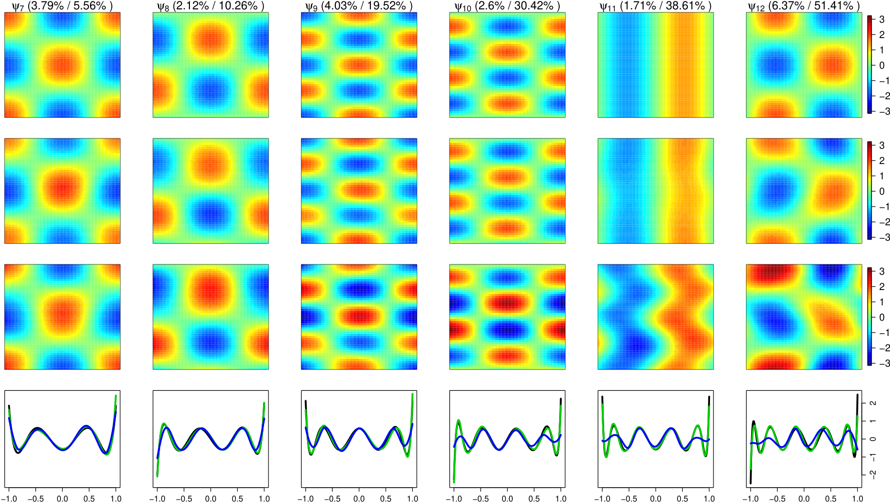
Figure 3: Relative errors for estimated eigenvalues (left) and eigenfunctions (right, log-scale) for simulation setting 3, depending on measurement error and univariate expansions.

The overall results for the first M=12M=12 eigenvalue/eigenvector pairs are given in Fig. 3. Compared to the settings with one-dimensional domain, the errors are slightly higher, in particular for higher order eigenvalues and eigenfunctions. Exemplary results however, show that even in this case, the new approach is still able to capture the important features of the true eigenfunctions well (see online appendix). The results further show that the general approach with spline basis functions performs mostly better than the pure MFPCA approach. Moreover, the truncated Karhunen-Loève representation with M=12M=12 (true M=25M=25) estimated eigenfunctions and scores gives an excellent reconstruction of the original data. The average MRSE\operatorname{MRSE} is 1.382%1.382\%/0.398%0.398\% (PCA/splines) for data without measurement error and 2.233%2.233\%/2.048%2.048\% (PCA/splines) for data with measurement error.

5 Application – ADNI Study

In this section, the new method is applied to data from the Alzheimer’s Disease Neuroimaging Initiative study (ADNI), which aims at identifying biomarkers for accurate diagnosis of Alzheimer’s disease (AD) in an early stage (Mueller et al.,, 2005). We use MFPCA to explore how longitudinal trajectories of a neuropsychological score (ADAS-Cog, a current standard for monitoring AD progression) covary with FDG-PET scans at baseline. The latter are used to assess the glucose metabolism in the brain, which is tightly coupled with neuronal function. As the brain images might be predictive of subsequent cognitive decline, common patterns between these two sources of information would be highly relevant.

Dataset: The dataset considered for MFPCA contains data from all N=483N=483 participants enrolled in ADNI1, having an FDG-PET scan at baseline and at least three ADAS-Cog measurements during follow-up. At baseline, 8484 subjects were diagnosed with AD, 302302 were suffering from mild cognitive impairment (MCI, in many cases an early stage of AD) and 9797 were cognitively healthy elderly controls. The ADAS-Cog trajectories constitute the first element X(1)X^{(1)}, where high values indicate a high level of cognitive impairment. The measurements contain missings, mostly in the second half of the study period and thus are sparse. The second element X(2)X^{(2)} is an axial slice of 93×11793\times 117 pixels (139.5 ×\times 175.5 mm2\text{mm}^{2}) of FDG-PET scans, containing the Precuneus and temporo-parietal regions. Both are believed to show a strong relation between hypometabolism (reduced brain function) and AD (Blennow et al.,, 2006). Exemplary data is shown in Fig. 4.

Figure 4: Left: ADAS-Cog trajectories for all N=483N=483 subjects. Numbers above the x-axis give the total number of measurements for each visit. Right: FDG-PET scans for three randomly chosen male subjects (left to right: AD, MCI, normal; diagnosis at baseline).

Weighted scalar product: As the ADAS-Cog trajectories and FDG-PET scans differ considerably in domain, range and variation (cf. Fig. 4), we use a weighted MFPCA with

wj=(∫𝒯jC^j​j(tj,tj)dtj)−1=(∫𝒯jVar^(X(j)(tj))dtj)−1,j=1,2,w_{j}=\left(\int_{\mathcal{T}_{j}}\hat{C}_{jj}(t_{j},t_{j})\mathrm{d}t_{j}\right)^{-1}=\left(\int_{\mathcal{T}_{j}}\widehat{\operatorname{Var}}\left(X^{(j)}(t_{j})\right)\mathrm{d}t_{j}\right)^{-1},\quad j=1,2,

where C^j​j\hat{C}_{jj} is estimated from the data. Using these weights, the integrated variance equals 11 for the rescaled elements X~(j)=wj1/2​X(j)\tilde{X}^{(j)}=w_{j}^{1/2}X^{(j)}. All elements thus contribute equal amounts of variation to the analysis, similarly to multivariate PCA, where the data is usually standardized before the analysis. We believe that this a sensible choice for many applications, but there may of course be situations, in which other weighting schemes may be preferable. For example, one could think of data that has two image elements, representing brain regions of different size for the same imaging modality. Here variability is naturally on the same scale and it might be better to keep the information of the site of the individual domains by setting both weights to one. On the other hand, if the images stem from different imaging modalities on the same domain, it might be necessary to correct solely for differences in variation. As a general rule, the weights should be chosen in close coordination with practitioners, considering the objective of the analysis and the data at hand.

Results: The results for the first two multivariate functional principal components, that account for 80.7%80.7\% of the total weighted variance, are shown in Fig. 5. For the univariate expansions, we use FPCA for X(1)X^{(1)} with M1=3M_{1}=3 principal components (explaining 99.2%99.2\% of the univariate variance) and 20×1520\times 15 tensor product B-splines for the images X(2)X^{(2)}. Fig. 5 further includes pointwise bootstrap confidence bands for the principal components based on 100100 nonparametric bootstrap iterations on the level of subjects. The coverage of such confidence bands for data consisting of functions and images has been analyzed in a simulation study, which gave good results, even in the presence of measurement error (see online appendix). The entire analysis for the ADNI data took around 1515 minutes on a standard laptop (2.7 GHz, 16 GB RAM) including the calculation of the bootstrap confidence bands and without parallelization.

Almost half of the variability in the data (46.7%46.7\% of the weighted variance) is explained by the first functional principal component. The ADAS-Cog element – and hence the degree of cognitive impairment – is elevated relative to the mean and increases during follow-up. The FDG-PET element exhibits hypometabolism in the Precuneus and the temporo-parietal regions, i.e. this component reflects reduced brain activity in these regions already at baseline. In total, the first eigenfunction seems to be interpretable as an AD related effect, as the pattern for positive scores perfectly agrees with medical knowledge about AD progression. This interpretation is supported by the estimated scores, which are mainly positive for people diagnosed with AD by their last visit, while scores of subjects who remained cognitively normal during follow-up are nearly all negative. Persons with MCI have intermediate score values, which is in line with the hypothesis that this diagnosis can constitute a transitional phase between normal ageing and AD.

For the second functional principal component (explains 33.9%33.9\% of weighted variance), the ADAS-Cog element is nearly constant and has wide bootstrap confidence bands that include zero during the whole follow-up. In contrast, the FDG-PET element differs significantly from zero in almost all voxels (cf. Fig. 5). Hence, this principal component reflects variation in the FDG-PET scans at baseline. Plotting the overall mean plus or minus this component suggests that it can be interpreted as an effect of imperfect registration that manifests in different brain sizes, which are known to correlate with gender (Ruigrok et al.,, 2014). This hypothesis is supported by the boxplots of the estimated scores in Fig. 5, while scores do not differ notably by diagnosis (not shown here).

Discussion: The results show that MFPCA is able to capture important sources of variation in the data that have a meaningful interpretation from a medical and neuroimaging point of view. An important issue not addressed here is that for ADAS-Cog, there may well be an informative dropout of patients with high score values (cf. Fig. 4). While addressing informative missingness goes beyond the scope of this paper, interpretation of results should take this possibility into account. For instance, it is easily conceivable that ψ^1(1)\hat{\psi}_{1}^{(1)} may be underestimating ψ1(1)\psi_{1}^{(1)} towards the end of the study period.

Figure 5: The first two estimated multivariate functional principal components for the ADNI data (1st row: ψ^1\hat{\psi}_{1}, 2nd row: ψ^2\hat{\psi}_{2}). Estimates are given with pointwise 95%95\% and 90%90\% bootstrap confidence bands based on 100100 nonparametric bootstrap iterations (ADAS-Cog, 1st column: Dashed lines; FDG-PET, 2nd and 3rd column: Pixels with pointwise 95%95\% (left) and 90%90\% (right) confidence bands not including zero in color). Boxplots of the scores (4th column) support the interpretation.

6 Discussion and Outlook

This paper introduces methodology and a practical estimation algorithm for multivariate functional principal component analysis. While other methods for MFPCA are restricted to observations on a common, one-dimensional interval, the new approach is suitable for data on different domains, which may also differ in dimension, such as functions and images. The key results are 1. a Karhunen-Loève Theorem, that establishes the theoretical basis for MFPCA (Prop. 4), 2. an explicit relation between multivariate and univariate FPCA, which serves as a starting point for the estimation (Prop. 5) and 3. asymptotic results for the estimators (Prop. 6 and 7). The estimation algorithm can be extended to expansions of the univariate elements in not necessarily orthonormal bases. This allows to flexibly choose an appropriate basis for each element depending on the data structure, in particular also mixtures of univariate FPCA and general bases. The algorithm is applicable to sparse data or data with measurement error, as well as to images. Notably, the proposed method can be used to calculate smooth univariate functional principal components for data on higher dimensional domains and is hence an alternative to existing methods for tensor PCA (Allen,, 2013). The results of MFPCA give insights into simultaneous variation within the data and provide a natural tool for dimension reduction. Moreover, they can be used as a building block for further statistical analyses such as functional clustering methods or functional principal component regression with multiple covariates (cf. Müller and Stadtmüller,, 2005, for the univariate case). If the elements differ in domain, range or variation, the new method can incorporate weights, which should be chosen with respect to the question of interest and the data at hand.

Possible extensions of the approach include normalization methods as an alternative to the weighted scalar product, following the ideas in Jacques and Preda, (2014) or Chiou et al., (2014) for functions observed on a common interval. However, one should take into account that the domains may have different dimensions and sizes. The concept of MFPCA could further be extended to hybrid data, i.e. data consisting of a functional and a vector part (Ramsay and Silverman,, 2005, Chapter 10.3.). A natural starting point would be to extend the scalar product suggested by Ramsay and Silverman, (2005) in this context to multivariate functional data as proposed in Prop. 1. However, transferring the results for MFPCA shown in this paper requires a careful revision of the concept of the covariance operator and related proofs. Finally, one could think of estimating the multivariate covariance operator directly without computing a univariate decomposition for each element. This operator is typically high-dimensional, making smoothing as well as an eigendecomposition hardly feasible, which is avoided in our two-step approach.

Supplementary Material

The online appendix contains detailed proofs for all propositions, some additional simulation results and R code for reproducing the analysis for the ADNI and gait cycle data based on the R packages fundata and MFPCA (Happ, 2016a, ; Happ, 2016b, ).

References

  • Allen, (2013) Allen, G. (2013). Multi-way functional principal components analysis. In IEEE 5th International Workshop on Computational Advances in Multi-Sensor Adaptive Processing (CAMSAP), pages 220–223.
  • Berrendero et al., (2011) Berrendero, J., Justel, A., and Svarc, M. (2011). Principal components for multivariate functional data. Computational Statistics & Data Analysis, 55(9):2619–2634.
  • Blennow et al., (2006) Blennow, K., Leon, M., and Zetterberg, H. (2006). Alzheimer’s disease. Lancet, 368:387–403.
  • Bosq, (2000) Bosq, D. (2000). Linear Processes in Function Spaces. Springer, New York.
  • Carroll and Chang, (1970) Carroll, J. D. and Chang, J. J. (1970). Analysis of individual differences in multidimensional scaling via an n-way generalization of ”Eckart-Young” decomposition. Psychometrika, 35(3):283–319.
  • Cattell, (1966) Cattell, R. (1966). The scree test for the number of factors. Multivariate Behavioral Research, 1(2):245–276.
  • Chiou et al., (2014) Chiou, J.-M., Yang, Y.-F., and Chen, Y.-T. (2014). Multivariate functional principal component analysis: A normalization approach. Statistica Sinica, 24:1571–1596.
  • Coppi and Bolasco, (1989) Coppi, R. and Bolasco, S., editors (1989). Multiway data analysis. North-Holland, Amsterdam.
  • Crainiceanu et al., (2014) Crainiceanu, C., Reiss, P., Goldsmith, J., Huang, L., Huo, L., and Scheipl, F. (2014). refund: Regression with Functional Data. R package version 0.1-14.
  • Eilers and Marx, (1996) Eilers, P. and Marx, B. (1996). Flexible Smoothing with B-splines and Penalties. Statistical Science, 11(2):89–121.
  • Hall and Horowitz, (2007) Hall, P. and Horowitz, J. L. (2007). Methodology and convergence rates for functional linear regression. Annals of Statistics, 35(1):70–91.
  • Hall and Hosseini-Nasab, (2006) Hall, P. and Hosseini-Nasab, M. (2006). On properties of functional principal components analysis. Journal of the Royal Statistical Society: Series B (Statistical Methodology), 68(1):109–126.
  • (13) Happ, C. (2016a). funData: An S4 class for functional data in R. R package version 1.0.
  • (14) Happ, C. (2016b). MFPCA: Multivariate Functional Principal Component Analysis. R package version 1.0-1.
  • Horn and Johnson, (1991) Horn, R. A. and Johnson, C. R. (1991). Topics in matrix analysis. Cambridge Univ. Press, Cambridge.
  • Huang et al., (2009) Huang, J. Z., Shen, H., and Buja, A. (2009). The Analysis of Two-Way Functional Data Using Two-Way Regularized Singular Value Decompositions. Journal of the American Statistical Association, 104(488):1609–1620.
  • Jacques and Preda, (2014) Jacques, J. and Preda, C. (2014). Model-based clustering for multivariate functional data. Computational Statistics & Data Analysis, 71:92–106.
  • Kato, (1976) Kato, T. (1976). Perturbation Theory for Linear Operators. Springer, Berlin, 2. edition.
  • Lu et al., (2013) Lu, H., Plataniotis, K. N., and Venetsanopoulos, A. (2013). Multilinear Subspace Learning: Dimensionality Reduction of Multidimensional Data. CRC press, Boca Raton.
  • Mercer, (1909) Mercer, J. (1909). Functions of Positive and Negative Type, and their Connection with the Theory of Integral Equations. Philosophical Transactions A, 209(441-458):415–446.
  • Mueller et al., (2005) Mueller, S., Weiner, M., Thal, L., Petersen, R., Jack, C., Jagust, W., Trojanowski, J., Toga, A., and Beckett, L. (2005). Ways toward an early diagnosis in Alzheimer’s disease: The Alzheimer’s Disease Neuroimaging Initiative (ADNI). Alzheimer’s & Dementia, 1(1):55–66.
  • Müller and Stadtmüller, (2005) Müller, H. G. and Stadtmüller, U. (2005). Generalized functional linear models. Annals of Statistics, 33(2):774–805.
  • Munkres, (2000) Munkres, J. (2000). Topology. Prentice-Hall, Upper Saddle River, NJ, 2. edition.
  • Ramsay and Silverman, (2005) Ramsay, J. and Silverman, B. (2005). Functional Data Analysis. Springer, New York, 2. edition.
  • Ramsay et al., (2014) Ramsay, J., Wickham, H., Graves, S., and Hooker, G. (2014). fda: Functional Data Analysis. R package version 2.4.4.
  • Reed and Simon, (1980) Reed, M. and Simon, B. (1980). Methods of Modern Mathematical Physics. I: Functional Analysis. Academic Press, San Diego, rev. and enl. edition.
  • Rudin, (1987) Rudin, W. (1987). Real and complex analysis. McGraw-Hill, New York, 3. edition.
  • Ruigrok et al., (2014) Ruigrok, A., Salimi-Khorshidi, G., Lai, M.-C., Baron-Cohen, S., Lombardo, M., Tait, R., and Suckling, J. (2014). A meta-analysis of sex differences in human brain structure. Neuroscience and biobehavioral reviews, 39:34–50.
  • Saporta, (1981) Saporta, G. (1981). Méthodes exploratoires d’analyse de données temporelles. PhD thesis, Université Pierre et Marie Curie, Paris.
  • Tucker, (1966) Tucker, L. R. (1966). Some Mathematical Notes on Three-Mode Factor Analysis. Psychometrika, 31(3):279–311.
  • Werner, (2011) Werner, D. (2011). Funktionalanalysis. Springer, Berlin, 7. edition.
  • Yao et al., (2005) Yao, F., Müller, H.-G., and Wang, J.-L. (2005). Functional data analysis for sparse longitudinal data. Journal of the American Statistical Association, 100(470):577–590.
  • Yu et al., (2015) Yu, Y., Wang, T., and Samworth, R. J. (2015). A useful variant of the Davis-Kahan theorem for statisticians. Biometrika, 102(2):315–323.
  • Zemyan, (2012) Zemyan, S. (2012). The Classical Theory of Integral Equations. Birkhäuser, Basel.

Proofs of Propositions

Proof of Prop. 1.

ℋ\mathcal{H} is a direct sum of the Hilbert spaces L2​(𝒯j),j=1,…,pL^{2}(\mathcal{T}_{j}),\penalty\ j=1,\ldots,p, with natural scalar product ⟨⟨⋅,⋅⟩⟩\langle\kern-1.07639pt\langle\cdot,\cdot\rangle\kern-1.07639pt\rangle (cf. Reed and Simon,, 1980, Chapter II.1.) ∎

Proof of Prop. 2.
  1. 1.

    Γ\Gamma is linear: Follows from the linearity of the scalar product in (3).

  2. 2.

    Γ\Gamma is self-adjoint: Follows from the symmetry Ci​j​(si,tj)=Cj​i​(tj,si)C_{ij}(s_{i},t_{j})=C_{ji}(t_{j},s_{i}).

  3. 3.

    Γ\Gamma is positive: Let f∈ℋf\in\mathcal{H}. Then

    ⟨⟨f,Γ​f⟩⟩\displaystyle\langle\kern-1.07639pt\langle f,\Gamma f\rangle\kern-1.07639pt\rangle =∑j=1p∫𝒯jf(j)​(tj)​∑i=1p∫𝒯i𝔼⁡(X(i)​(si)​X(j)​(tj))​f(i)​(si)​d​si​d​tj\displaystyle=\sum\nolimits_{j=1}^{p}\int_{\mathcal{T}_{j}}f^{(j)}(t_{j})\sum\nolimits_{i=1}^{p}\int_{\mathcal{T}_{i}}\mathbb{E}\left(X^{(i)}(s_{i})X^{(j)}(t_{j})\right)f^{(i)}(s_{i})\mathrm{d}s_{i}\penalty\ \mathrm{d}t_{j}
    =𝔼​(∑j=1p∫𝒯jf(j)​(tj)​X(j)​(tj)​d​tj)2≥0.\displaystyle=\mathbb{E}\left(\sum\nolimits_{j=1}^{p}\int_{\mathcal{T}_{j}}f^{(j)}(t_{j})X^{(j)}(t_{j})\mathrm{d}t_{j}\right)^{2}\geq 0.
  4. 4.

    Γ\Gamma is compact: Let ℬ:={f∈ℋ:‖|f|‖2≤B}\mathcal{B}:=\{f\in\mathcal{H}:{\left|\kern-1.07639pt\left|\kern-1.07639pt\left|f\right|\kern-1.07639pt\right|\kern-1.07639pt\right|}^{2}\leq B\} be a bounded family in ℋ\mathcal{H} for some constant 0<B<∞0<B<\infty. Clearly, ‖f(j)‖22≤B{\left|\kern-1.07639pt\left|f^{(j)}\right|\kern-1.07639pt\right|_{2}}^{2}\leq B for all j=1,…,pj=1,\ldots,p. Define the image of ℬ\mathcal{B} under Γ\Gamma by 𝒵=Γ​ℬ={g∈ℋ:∃f∈ℬ​ such that ​g=Γ​f}\mathcal{Z}=\Gamma\mathcal{B}=\{g\in\mathcal{H}:\exists\penalty\ f\in\mathcal{B}\text{ such that }g=\Gamma f\}, which has the following properties:

    • •

      𝒵\mathcal{Z} is uniformly bounded: Let g∈𝒵g\in\mathcal{Z} and 𝒕∈𝒯\boldsymbol{t}\in\mathcal{T}. Define K:=maxi,j=1,…,p⁡Ki​jK:=\max\nolimits_{i,j=1,\ldots,p}K_{ij} with Ki​jK_{ij} as in (5). Then

      ‖g⁡(𝒕)‖2\displaystyle{\left|\kern-1.07639pt\left|g(\boldsymbol{t})\right|\kern-1.07639pt\right|}^{2} ≤∑j=1p(∑i=1p∫𝒯i|Ci​j​(si,tj)​f(i)​(si)|​d​si)2\displaystyle\leq\sum\nolimits_{j=1}^{p}\left(\sum\nolimits_{i=1}^{p}\int_{\mathcal{T}_{i}}\left|C_{ij}(s_{i},t_{j})f^{(i)}(s_{i})\right|\mathrm{d}s_{i}\right)^{2}
      ≤Hölder∑j=1p(∑i=1p[∫𝒯iCi​j​(si,tj)2​d​si]1/2​[∫𝒯if(i)​(si)2​d​si]1/2)2\displaystyle\stackrel{{\scriptstyle\text{H\"{o}lder}}}{{\leq}}\sum\nolimits_{j=1}^{p}\left(\sum\nolimits_{i=1}^{p}\left[\int_{\mathcal{T}_{i}}C_{ij}(s_{i},t_{j})^{2}\mathrm{d}s_{i}\right]^{1/2}\left[\int_{\mathcal{T}_{i}}f^{(i)}(s_{i})^{2}\mathrm{d}s_{i}\right]^{1/2}\right)^{2}
      ≤∑j=1p(∑i=1pK1/2​B1/2)2=p3​K​B<∞.\displaystyle\leq\sum\nolimits_{j=1}^{p}\left(\sum\nolimits_{i=1}^{p}K^{1/2}B^{1/2}\right)^{2}=p^{3}KB<\infty.
    • •

      𝒵\mathcal{Z} is equicontinuous: Denote by λ⁡(𝒯j)\lambda(\mathcal{T}_{j}) the Lebesgue measure of 𝒯j\mathcal{T}_{j} and let T=maxj=1,…,p⁡λ⁡(𝒯j)T=\max\nolimits_{j=1,\ldots,p}\lambda(\mathcal{T}_{j}). For ε>0\varepsilon>0, define ε~:=εp​(p​T​B)1/2\tilde{\varepsilon}:=\frac{\varepsilon}{p(pTB)^{1/2}}. By the continuity assumption for Ci​j​(si,⋅)C_{ij}(s_{i},\cdot), there exist δi​j>0\delta_{ij}>0 such that

      ‖tj−tj∗‖<δi​j⇒|Ci​j​(si,tj)−Ci​j​(si,tj∗)|<ε~,∀si∈𝒯i.{\left|\kern-1.07639pt\left|t_{j}-t^{\ast}_{j}\right|\kern-1.07639pt\right|}<\delta_{ij}\quad\Rightarrow\quad|C_{ij}(s_{i},t_{j})-C_{ij}(s_{i},t_{j}^{\ast})|<\tilde{\varepsilon},\quad\forall\penalty\ s_{i}\in\mathcal{T}_{i}. (12)

      for all i,j=1,…,pi,j=1,\ldots,p. Set δ:=mini,j=1,…,p⁡δi​j\delta:=\min\nolimits_{i,j=1,\ldots,p}\delta_{ij} and let ‖𝒕−𝒕∗‖𝒯<δ{\left|\kern-1.07639pt\left|\boldsymbol{t}-\boldsymbol{t^{\ast}}\right|\kern-1.07639pt\right|}_{\mathcal{T}}<\delta. Clearly, ‖tj−tj∗‖<δ{\left|\kern-1.07639pt\left|t_{j}-t_{j}^{\ast}\right|\kern-1.07639pt\right|}<\delta for all j=1,…,pj=1,\ldots,p and for g∈𝒵g\in\mathcal{Z} it holds

      ‖g⁡(𝒕)−g⁡(𝒕∗)‖2≤∑j=1p(∑i=1p|∫𝒯i(Ci​j​(si,tj)−Ci​j​(si,tj∗))​f(i)​(si)​d​si|)2\displaystyle{\left|\kern-1.07639pt\left|g(\boldsymbol{t})-g(\boldsymbol{t^{\ast}})\right|\kern-1.07639pt\right|}^{2}\leq\sum\nolimits_{j=1}^{p}\left(\sum\nolimits_{i=1}^{p}\left|\int_{\mathcal{T}_{i}}\left(C_{ij}(s_{i},t_{j})-C_{ij}(s_{i},t_{j}^{\ast})\right)f^{(i)}(s_{i})\mathrm{d}s_{i}\right|\right)^{2}
      ≤Hölder∑j=1p(∑i=1p[∫𝒯i(Ci​j​(si,tj)−Ci​j​(si,tj∗))2​d​si]1/2​[∫𝒯if(i)​(si)2​d​si]1/2)2\displaystyle\quad\penalty\ \penalty\ \stackrel{{\scriptstyle\text{H\"{o}lder}}}{{\leq}}\sum\nolimits_{j=1}^{p}\left(\sum\nolimits_{i=1}^{p}\left[\int_{\mathcal{T}_{i}}\left(C_{ij}(s_{i},t_{j})-C_{ij}(s_{i},t_{j}^{\ast})\right)^{2}\mathrm{d}s_{i}\right]^{1/2}\left[\int_{\mathcal{T}_{i}}f^{(i)}(s_{i})^{2}\mathrm{d}s_{i}\right]^{1/2}\right)^{2}
      <(12)∑j=1p(∑i=1p(∫𝒯iε~2​d​si)1/2​‖f(i)‖2)2≤p3​T​B​ε~2=ε2.\displaystyle\qquad\stackrel{{\scriptstyle\eqref{eq:CovCont}}}{{<}}\sum\nolimits_{j=1}^{p}\left(\sum\nolimits_{i=1}^{p}\left(\int_{\mathcal{T}_{i}}\tilde{\varepsilon}^{2}\mathrm{d}s_{i}\right)^{1/2}{\left|\kern-1.07639pt\left|f^{(i)}\right|\kern-1.07639pt\right|_{2}}\right)^{2}\leq p^{3}TB\tilde{\varepsilon}^{2}=\varepsilon^{2}.

    By the Theorem of Arzelà-Ascoli (Reed and Simon,, 1980, Thm. I.28. and related notes for Chapter I), for each sequence {fn}n∈ℕ\{f_{n}\}_{n\in\mathbb{N}} in ℬ\mathcal{B} there exists a convergent subsequence {gn⁡(i)=Γfn⁡(i)}i∈ℕ\{g_{n(i)}=\Gamma f_{n(i)}\}_{i\in\mathbb{N}} of the corresponding sequence {gn}n∈ℕ\{g_{n}\}_{n\in\mathbb{N}} in 𝒵\mathcal{Z}, which implies that Γ\Gamma is a compact operator (cf. Reed and Simon,, 1980, Chapter VI.5.).

∎

Lemma 1.

For fixed m∈ℕm\in\mathbb{N} and j∈{1,…,p}j\in\{1,\ldots,p\}, the jj-th element ψm(j)\psi_{m}^{(j)} of the eigenfunction ψm\psi_{m} is continuous, if νm>0\nu_{m}>0 and Ci​jC_{ij} is uniformly continuous as in Prop. 2.

Proof.

Let ε>0\varepsilon>0 and ε~:=ε​νm​(2​∑j=1pλ​(𝒯j)1/2)−1\tilde{\varepsilon}:=\varepsilon\nu_{m}\left(2\sum_{j=1}^{p}\lambda(\mathcal{T}_{j})^{1/2}\right)^{-1}. By the uniform continuity assumption for Ci​jC_{ij}, there exist δi​j>0\delta_{ij}>0 such that for all i=1,…,pi=1,\ldots,p (12) holds. Let δj=mini=1,…,p⁡δi​j\delta_{j}=\min\nolimits_{i=1,\ldots,p}\delta_{ij} and ‖tj−tj∗‖<δj{\left|\kern-1.07639pt\left|t_{j}-t_{j}^{\ast}\right|\kern-1.07639pt\right|}<\delta_{j}. Then, as νm>0\nu_{m}>0 and ‖ψm(i)‖2≤‖|ψm|‖=1{\left|\kern-1.07639pt\left|\psi_{m}^{(i)}\right|\kern-1.07639pt\right|_{2}}\leq{\left|\kern-1.07639pt\left|\kern-1.07639pt\left|\psi_{m}\right|\kern-1.07639pt\right|\kern-1.07639pt\right|}=1,

|ψm(j)​(tj)−ψm(j)​(tj∗)|=1νm​|∑i=1p∫𝒯i[Ci​j​(si,tj)−Ci​j​(si,tj∗)]​ψm(i)​(si)​d​si|\displaystyle\left|\psi_{m}^{(j)}(t_{j})-\psi_{m}^{(j)}(t_{j}^{\ast})\right|=\frac{1}{\nu_{m}}\penalty\ \left|\sum\nolimits_{i=1}^{p}\int_{\mathcal{T}_{i}}\left[C_{ij}(s_{i},t_{j})-C_{ij}(s_{i},t_{j}^{\ast})\right]\psi_{m}^{(i)}(s_{i})\mathrm{d}s_{i}\right|
≤1νm​ε~​∑i=1p∫𝒯i|ψm(i)​(si)|​d​si≤Hölderε~νm​∑i=1p‖ψm(i)‖2​λ​(𝒯i)1/2\displaystyle\qquad\leq\frac{1}{\nu_{m}}\tilde{\varepsilon}\penalty\ \sum\nolimits_{i=1}^{p}\int_{\mathcal{T}_{i}}\left|\psi_{m}^{(i)}(s_{i})\right|\mathrm{d}s_{i}\stackrel{{\scriptstyle\text{H\"{o}lder}}}{{\leq}}\frac{\tilde{\varepsilon}}{\nu_{m}}\penalty\ \sum\nolimits_{i=1}^{p}{\left|\kern-1.07639pt\left|\psi_{m}^{(i)}\right|\kern-1.07639pt\right|_{2}}\lambda(\mathcal{T}_{i})^{1/2}
≤ε~νm​∑i=1pλ​(𝒯i)1/2=ε2<ε.\displaystyle\qquad\leq\frac{\tilde{\varepsilon}}{\nu_{m}}\penalty\ \sum\nolimits_{i=1}^{p}\lambda(\mathcal{T}_{i})^{1/2}=\frac{\varepsilon}{2}<\varepsilon.

∎

Proof of Prop. 3.

The proof follows the idea in Werner, (2011, Chapter VI.4.) for the proof of Mercer’s Theorem in the univariate case. From the Spectral Theorem for compact self-adjoint operators (Werner,, 2011, Thm. VI.3.2.), it is known that

Γ​f=∑m=1∞νm​⟨⟨f,ψm⟩⟩​ψm∀f∈ℋ.\Gamma f=\sum\nolimits_{m=1}^{\infty}\nu_{m}\langle\kern-1.07639pt\langle f,\psi_{m}\rangle\kern-1.07639pt\rangle\psi_{m}\quad\forall\penalty\ f\in\mathcal{H}.

For M∈ℕM\in\mathbb{N} define

ΓM​f:=∑m=1Mνm​⟨⟨f,ψm⟩⟩​ψm∀f∈ℋ.\Gamma_{M}f:=\sum\nolimits_{m=1}^{M}\nu_{m}\langle\kern-1.07639pt\langle f,\psi_{m}\rangle\kern-1.07639pt\rangle\psi_{m}\quad\forall\penalty\ f\in\mathcal{H}.

Then for all f∈ℋ:⟨⟨Γ​f,f⟩⟩−⟨⟨ΓM​f,f⟩⟩=∑m=M+1∞νm​⟨⟨f,ψm⟩⟩2≥0f\in\mathcal{H}:\penalty\ \langle\kern-1.07639pt\langle\Gamma f,f\rangle\kern-1.07639pt\rangle-\langle\kern-1.07639pt\langle\Gamma_{M}f,f\rangle\kern-1.07639pt\rangle=\sum\nolimits_{m=M+1}^{\infty}\nu_{m}\langle\kern-1.07639pt\langle f,\psi_{m}\rangle\kern-1.07639pt\rangle^{2}\geq 0. Let j∈{1,…,p}j\in\{1,\ldots,p\} and t∗∈𝒯jt^{\ast}\in\mathcal{T}_{j}. Define f=(0,…,0,f(j),0,…,0)f=\left(0,\ldots,0,f^{(j)},0,\ldots,0\right) with f(j)=λ​(Bt∗​(1n))−1​𝟏Bt∗​(1n)f^{(j)}=\lambda\left(B_{t^{\ast}}\left(\frac{1}{n}\right)\right)^{-1}\boldsymbol{1}_{B_{t^{\ast}}(\frac{1}{n})} for some n∈ℕn\in\mathbb{N}, where Bt∗​(1n)B_{t^{\ast}}(\frac{1}{n}) is a closed ball in 𝒯j\mathcal{T}_{j} with center t∗t^{\ast} and radius 1n\frac{1}{n}, λ⁡(⋅)\lambda(\cdot) denotes the Lebesgue measure and 𝟏\boldsymbol{1} is the indicator function. Clearly, f(j)∈L2​(𝒯j)f^{(j)}\in L^{2}(\mathcal{T}_{j}) and f∈ℋf\in\mathcal{H}. Therefore

0\displaystyle 0 ≤⟨⟨Γ​f,f⟩⟩−⟨⟨ΓM​f,f⟩⟩\displaystyle\leq\langle\kern-1.07639pt\langle\Gamma f,f\rangle\kern-1.07639pt\rangle-\langle\kern-1.07639pt\langle\Gamma_{M}f,f\rangle\kern-1.07639pt\rangle
=λ​(Bt∗​(1n))−2​∫Bt∗​(1n)∫Bt∗​(1n)Cj​j​(sj,tj)−∑m=1Mνm​ψm(j)​(sj)​ψm(j)​(tj)​d​sj​d​tj\displaystyle=\lambda\left(B_{t^{\ast}}\left(\tfrac{1}{n}\right)\right)^{-2}\int_{B_{t^{\ast}}(\frac{1}{n})}\int_{B_{t^{\ast}}(\frac{1}{n})}C_{jj}(s_{j},t_{j})-\sum\nolimits_{m=1}^{M}\nu_{m}\psi_{m}^{(j)}(s_{j})\psi_{m}^{(j)}(t_{j})\mathrm{d}s_{j}\penalty\ \mathrm{d}t_{j}
→Cj​j​(t∗,t∗)−∑m=1Mνm​ψm(j)​(t∗)​ψm(j)​(t∗)for​n→∞\displaystyle\to C_{jj}(t^{\ast},t^{\ast})-\sum\nolimits_{m=1}^{M}\nu_{m}\psi_{m}^{(j)}(t^{\ast})\psi_{m}^{(j)}(t^{\ast})\quad\text{for}\penalty\ n\to\infty

by the Lebesgue Differentiation Theorem (Rudin,, 1987, Thm. 7.10.). As t∗t^{\ast} was arbitrary in 𝒯j\mathcal{T}_{j}, this implies that for all M∈ℕM\in\mathbb{N}

∑m=1Mνm​ψm(j)​(t)2≤Cj​j​(t,t)≤‖Cj​j‖∞<∞∀t∈𝒯j,\sum\nolimits_{m=1}^{M}\nu_{m}\psi_{m}^{(j)}(t)^{2}\leq C_{jj}(t,t)\leq\left\|C_{jj}\right\|_{\infty}<\infty\quad\forall\penalty\ t\in\mathcal{T}_{j},

since Cj​jC_{jj} is continuous and 𝒯j\mathcal{T}_{j} is compact, implying that ‖Cj​j‖∞:=supt∈𝒯j|Cj​j​(t,t)|\left\|C_{jj}\right\|_{\infty}:=\sup_{t\in\mathcal{T}_{j}}\left|C_{jj}(t,t)\right| is finite. Using Hölder’s inequality

∑m=1∞|νm​ψm(j)​(s)​ψm(j)​(t)|≤Cj​j​(s,s)1/2​Cj​j​(t,t)1/2<∞,\sum\nolimits_{m=1}^{\infty}\left|\nu_{m}\psi_{m}^{(j)}(s)\psi_{m}^{(j)}(t)\right|\leq C_{jj}(s,s)^{1/2}C_{jj}(t,t)^{1/2}<\infty,

i.e. the series C~j​(s,t):=∑m=1∞νm​ψm(j)​(s)​ψm(j)​(t)\tilde{C}_{j}(s,t):=\sum\nolimits_{m=1}^{\infty}\nu_{m}\psi_{m}^{(j)}(s)\psi_{m}^{(j)}(t) is absolutely convergent for all s,t∈𝒯js,t\in\mathcal{T}_{j}. In the following, assume t∈𝒯jt\in\mathcal{T}_{j} to be fixed. For ε>0\varepsilon>0 choose M∈ℕM\in\mathbb{N} such that ∑m=M+1∞νm​ψm(j)​(t)2<ε2\sum\nolimits_{m=M+1}^{\infty}\nu_{m}\psi_{m}^{(j)}(t)^{2}<\varepsilon^{2}. Then, again by Hölder’s inequality

∑m=M+1∞|νm​ψm(j)​(s)​ψm(j)​(t)|\displaystyle\sum\nolimits_{m=M+1}^{\infty}\left|\nu_{m}\psi_{m}^{(j)}(s)\psi_{m}^{(j)}(t)\right| ≤Cj​j​(s,s)1/2⋅ε≤‖Cj​j‖∞1/2⋅ε.\displaystyle\leq C_{jj}(s,s)^{1/2}\cdot\varepsilon\leq\left\|C_{jj}\right\|_{\infty}^{1/2}\cdot\varepsilon. (13)

The upper bound in (13) does not depend on ss, hence C~j​(s,t)\tilde{C}_{j}(s,t) converges uniformly for fixed tt. As the eigenfunctions ψm(j)​(s)\psi_{m}^{(j)}(s) are continuous in ss for all m∈ℕm\in\mathbb{N} (Lemma 1), C~j​(s,t)\tilde{C}_{j}(s,t) is also continuous in ss (Uniform Limit Theorem, Munkres,, 2000, Thm. 21.6.). Define

hj​(s):=Cj​j​(s,t)−C~j​(s,t),s∈𝒯j.h_{j}(s):=C_{jj}(s,t)-\tilde{C}_{j}(s,t),\quad s\in\mathcal{T}_{j}.

Let now g(j)∈L2​(𝒯j)g^{(j)}\in L^{2}(\mathcal{T}_{j}) and define g:=(0,…,0,g(j),0,…,0)g:=\left(0,\ldots,0,g^{(j)},0,\ldots,0\right), which is clearly in ℋ\mathcal{H}. Therefore

∫𝒯jhj​(s)​g(j)​(s)​𝑑s=∑i=1p∫𝒯iCi​j​(si,t)​g(i)​(si)​d​si−∑m=1∞νm​∑i=1p∫𝒯iψm(i)​(si)​g(i)​(si)​d​si​ψm(j)​(t)\displaystyle\int_{\mathcal{T}_{j}}h_{j}(s)g^{(j)}(s)\mathrm{d}s=\sum\nolimits_{i=1}^{p}\int_{\mathcal{T}_{i}}C_{ij}(s_{i},t)g^{(i)}(s_{i})\mathrm{d}s_{i}-\sum\nolimits_{m=1}^{\infty}\nu_{m}\sum\nolimits_{i=1}^{p}\int_{\mathcal{T}_{i}}\psi_{m}^{(i)}(s_{i})g^{(i)}(s_{i})\mathrm{d}s_{i}\penalty\ \psi_{m}^{(j)}(t)
=(Γ​g)(j)​(t)−∑m=1∞νm​⟨⟨ψm,g⟩⟩​ψm(j)​(t)\displaystyle\qquad=(\Gamma g)^{(j)}(t)-\sum\nolimits_{m=1}^{\infty}\nu_{m}\langle\kern-1.07639pt\langle\psi_{m},g\rangle\kern-1.07639pt\rangle\psi_{m}^{(j)}(t)
=∑m=1∞νm​⟨⟨g,ψm⟩⟩​ψm(j)​(t)−∑m=1∞νm​⟨⟨ψm,g⟩⟩​ψm(j)​(t)=0\displaystyle\qquad=\sum\nolimits_{m=1}^{\infty}\nu_{m}\langle\kern-1.07639pt\langle g,\psi_{m}\rangle\kern-1.07639pt\rangle\psi_{m}^{(j)}(t)-\sum\nolimits_{m=1}^{\infty}\nu_{m}\langle\kern-1.07639pt\langle\psi_{m},g\rangle\kern-1.07639pt\rangle\psi_{m}^{(j)}(t)=0

according to the Spectral Theorem. Choosing g(j)=hjg^{(j)}=h_{j} implies hj​(s)=0h_{j}(s)=0 for all s∈𝒯js\in\mathcal{T}_{j}, as hjh_{j} is continuous in ss. Therefore,

C~j​(s,t)=∑m=1∞νm​ψm(j)​(s)​ψm(j)​(t)=Cj​j​(s,t)∀s∈𝒯j.\tilde{C}_{j}(s,t)=\sum\nolimits_{m=1}^{\infty}\nu_{m}\psi_{m}^{(j)}(s)\psi_{m}^{(j)}(t)=C_{jj}(s,t)\quad\forall\penalty\ s\in\mathcal{T}_{j}.

By Dini’s Theorem (Werner,, 2011, Thm. VI.4.6.) the series Cj​j​(t,t)=∑m=1∞νm​ψm(j)​(t)2C_{jj}(t,t)=\sum\nolimits_{m=1}^{\infty}\nu_{m}\psi_{m}^{(j)}(t)^{2} converges uniformly. Hence, MM can be chosen independent of tt in (13). This implies that C~j​(s,t)\tilde{C}_{j}(s,t) converges absolutely and uniformly to Cj​j​(s,t)C_{jj}(s,t) for all s,t∈𝒯js,t\in\mathcal{T}_{j}. ∎

Proof of Prop. 4.

By the Hilbert-Schmidt Theorem (Reed and Simon,, 1980, Thm. VI.16.), the (deterministic) eigenfunctions of Γ\Gamma form an orthonormal basis of ℋ\mathcal{H}, i.e. XX can be written in the form X⁡(𝒕)=∑m=1∞ρm​ψm​(𝒕),𝒕∈𝒯X(\boldsymbol{t})=\sum\nolimits_{m=1}^{\infty}\rho_{m}\psi_{m}(\boldsymbol{t}),\penalty\ \boldsymbol{t}\in\mathcal{T} with random variables ρm=⟨⟨X,ψm⟩⟩\rho_{m}=\langle\kern-1.07639pt\langle X,\psi_{m}\rangle\kern-1.07639pt\rangle. Hence for m,n∈ℕm,n\in\mathbb{N}

  1. 1.

    𝔼⁡(ρm)=∑j=1p∫𝒯j𝔼⁡(X(j)​(tj))​ψm(j)​(tj)​d​tj=0,\mathbb{E}\left(\rho_{m}\right)=\displaystyle\sum\nolimits_{j=1}^{p}\displaystyle\int_{\mathcal{T}_{j}}\mathbb{E}\left(X^{(j)}(t_{j})\right)\psi_{m}^{(j)}(t_{j})\mathrm{d}t_{j}=0, since 𝔼⁡(X(j)​(tj))=0\mathbb{E}\left(X^{(j)}(t_{j})\right)=0 for all tj∈𝒯jt_{j}\in\penalty\ \mathcal{T}_{j}, j=1,…,pj=1,\ldots,p by assumption.

  2. 2.

    Cov⁡(ρm,ρn)=𝔼⁡(∑i=1p∫𝒯iX(i)​(si)​ψm(i)​(si)​d​si⋅∑j=1p∫𝒯jX(j)​(tj)​ψn(j)​(tj)​d​tj)=∑j=1p∫𝒯j∑i=1p∫𝒯iCi​j​(si,tj)​ψm(i)​(si)​d​si​ψn(j)​(tj)​d​tj=∑j=1p∫𝒯jνm​ψm(j)​(tj)​ψn(j)​(tj)​d​tj=νm​δm​n.\begin{aligned} &\operatorname{Cov}(\rho_{m},\rho_{n})=\mathbb{E}\left(\sum\nolimits_{i=1}^{p}\int_{\mathcal{T}_{i}}X^{(i)}(s_{i})\psi_{m}^{(i)}(s_{i})\mathrm{d}s_{i}\cdot\sum\nolimits_{j=1}^{p}\int_{\mathcal{T}_{j}}X^{(j)}(t_{j})\psi_{n}^{(j)}(t_{j})\mathrm{d}t_{j}\right)\\ &\qquad=\sum\nolimits_{j=1}^{p}\int_{\mathcal{T}_{j}}\sum\nolimits_{i=1}^{p}\int_{\mathcal{T}_{i}}C_{ij}(s_{i},t_{j})\psi_{m}^{(i)}(s_{i})\mathrm{d}s_{i}\penalty\ \psi_{n}^{(j)}(t_{j})\mathrm{d}t_{j}\\ &\qquad=\sum\nolimits_{j=1}^{p}\int_{\mathcal{T}_{j}}\nu_{m}\psi_{m}^{(j)}(t_{j})\psi_{n}^{(j)}(t_{j})\mathrm{d}t_{j}=\nu_{m}\delta_{mn}.\end{aligned}

  3. 3.

    Let X⌈M⌉​(𝒕):=∑m=1Mρm​ψm​(𝒕)=∑m=1M[∑i=1p∫𝒯iX(i)​(si)​ψm(i)​(si)​d​si]​ψm​(𝒕)X_{\lceil M\rceil}(\boldsymbol{t}):=\displaystyle\sum\nolimits_{m=1}^{M}\rho_{m}\psi_{m}(\boldsymbol{t})=\displaystyle\sum\nolimits_{m=1}^{M}\left[\displaystyle\sum\nolimits_{i=1}^{p}\displaystyle\int_{\mathcal{T}_{i}}X^{(i)}(s_{i})\psi_{m}^{(i)}(s_{i})\mathrm{d}s_{i}\right]\psi_{m}(\boldsymbol{t}) for 𝒕∈𝒯\boldsymbol{t}\in\penalty\ \mathcal{T} be the truncated Karhunen-Loève representation of XX. Then

    𝔼⁡(‖X⁡(𝒕)−X⌈M⌉​(𝒕)‖2)=∑j=1p[𝔼⁡(X(j)​(tj)2)−2​𝔼​(X(j)​(tj)​SM(j)​(tj))+𝔼⁡(SM(j)​(tj)2)]\displaystyle\mathbb{E}\left({\left|\kern-1.07639pt\left|X(\boldsymbol{t})-X_{\lceil M\rceil}(\boldsymbol{t})\right|\kern-1.07639pt\right|}^{2}\right)=\sum\nolimits_{j=1}^{p}\left[\mathbb{E}\left(X^{(j)}(t_{j})^{2}\right)-2\mathbb{E}\left(X^{(j)}(t_{j})S_{M}^{(j)}(t_{j})\right)+\mathbb{E}\left(S_{M}^{(j)}(t_{j})^{2}\right)\right]
    =∑j=1p[Cj​j(tj,tj)−2∑m=1M∑i=1p∫𝒯iCi​j(si,tj)ψm(i)(si)dsiψm(j)(tj)\displaystyle\qquad=\sum\nolimits_{j=1}^{p}\Big[C_{jj}(t_{j},t_{j})-2\sum\nolimits_{m=1}^{M}\sum\nolimits_{i=1}^{p}\int_{\mathcal{T}_{i}}C_{ij}(s_{i},t_{j})\psi_{m}^{(i)}(s_{i})\mathrm{d}s_{i}\penalty\ \psi_{m}^{(j)}(t_{j})
    +∑m=1M∑n=1M∑i=1p∫𝒯i∑k=1p∫𝒯kCk​i(uk,si)ψn(k)(uk)dukψm(i)(si)dsiψm(j)(tj)ψn(j)(tj)]\displaystyle\qquad\penalty\ \penalty\ +\sum\nolimits_{m=1}^{M}\sum\nolimits_{n=1}^{M}\sum\nolimits_{i=1}^{p}\int_{\mathcal{T}_{i}}\sum\nolimits_{k=1}^{p}\int_{\mathcal{T}_{k}}C_{ki}(u_{k},s_{i})\psi_{n}^{(k)}(u_{k})\mathrm{d}u_{k}\penalty\ \psi_{m}^{(i)}(s_{i})\mathrm{d}s_{i}\penalty\ \psi_{m}^{(j)}(t_{j})\psi_{n}^{(j)}(t_{j})\Big]
    =∑j=1p[Cj​j(tj,tj)−2∑m=1Mνmψm(j)(tj)ψm(j)(tj)\displaystyle\qquad=\sum\nolimits_{j=1}^{p}\Big[C_{jj}(t_{j},t_{j})-2\sum\nolimits_{m=1}^{M}\nu_{m}\psi_{m}^{(j)}(t_{j})\psi_{m}^{(j)}(t_{j})
    +∑m=1M∑n=1M∑i=1p∫𝒯iνnψn(i)(si)ψm(i)(si)dsiψm(j)(tj)ψn(j)(tj)]\displaystyle\qquad\penalty\ \penalty\ +\sum\nolimits_{m=1}^{M}\sum\nolimits_{n=1}^{M}\sum\nolimits_{i=1}^{p}\int_{\mathcal{T}_{i}}\nu_{n}\psi_{n}^{(i)}(s_{i})\psi_{m}^{(i)}(s_{i})\mathrm{d}s_{i}\psi_{m}^{(j)}(t_{j})\psi_{n}^{(j)}(t_{j})\Big]
    =∑j=1p[Cj​j​(tj,tj)−∑m=1Mνm​ψm(j)​(tj)2]→0for​M→∞\displaystyle\qquad=\sum\nolimits_{j=1}^{p}\left[C_{jj}(t_{j},t_{j})-\sum\nolimits_{m=1}^{M}\nu_{m}\psi_{m}^{(j)}(t_{j})^{2}\right]\to 0\quad\text{for}\penalty\ M\to\infty

    uniformly for 𝒕∈𝒯\boldsymbol{t}\in\mathcal{T} by Prop. 3.

∎

Proof of Prop. 5.
  1. 1.

    Let XX have a finite Karhunen-Loève representation (7). Then, each element is given by X(j)=∑m=1Mρm​ψm(j)X^{(j)}=\sum\nolimits_{m=1}^{M}\rho_{m}\psi_{m}^{(j)}. For t∈𝒯jt\in\mathcal{T}_{j}

    (Γ(j)​ϕ~(j))​(t)\displaystyle\left(\Gamma^{(j)}\tilde{\phi}^{(j)}\right)(t) =∫𝒯jCov⁡(X(j)​(s),X(j)​(t))​ϕ~(j)​(s)​𝑑s\displaystyle=\int_{\mathcal{T}_{j}}\operatorname{Cov}(X^{(j)}(s),X^{(j)}(t))\tilde{\phi}^{(j)}(s)\mathrm{d}s
    =∫𝒯j∑m=1Mνm​ψm(j)​(s)​ψm(j)​(t)​ϕ~(j)​(s)​𝑑s=!λ(j)​ϕ~(j)​(t),\displaystyle=\int_{\mathcal{T}_{j}}\sum\nolimits_{m=1}^{M}\nu_{m}\psi_{m}^{(j)}(s)\psi_{m}^{(j)}(t)\tilde{\phi}^{(j)}(s)\mathrm{d}s\stackrel{{\scriptstyle!}}{{=}}\lambda^{(j)}\tilde{\phi}^{(j)}(t), (14)

    which is a homogenous Fredholm integral equation of the second kind with separable kernel function K⁡(s,t)=∑m=1Mνm​ψm(j)​(s)​ψm(j)​(t)=∑m=1Mam​(s)​bm​(t)K(s,t)=\sum\nolimits_{m=1}^{M}\nu_{m}\psi_{m}^{(j)}(s)\psi_{m}^{(j)}(t)=\sum\nolimits_{m=1}^{M}a_{m}(s)b_{m}(t) with continuous functions am​(s)=νm1/2​ψm(j)​(s),bm​(t)=νm1/2​ψm(j)​(t)a_{m}(s)=\nu_{m}^{1/2}\psi_{m}^{(j)}(s),\penalty\ b_{m}(t)=\nu_{m}^{1/2}\psi_{m}^{(j)}(t) (cf. Lemma 1). Following the argumentation in Zemyan, (2012, Chapter 1.3.), (14) can be transformed into the matrix eigenequation

    𝑨(𝒋)​𝒖=λ(j)​𝒖\boldsymbol{A^{(j)}u}=\lambda^{(j)}\boldsymbol{u}

    with a symmetric matrix 𝑨(𝒋)∈ℝM×M\boldsymbol{A^{(j)}}\in\mathbb{R}^{M\times M} given by Am​n(j)=⟨am,bn⟩2A_{mn}^{(j)}={\langle a_{m},b_{n}\rangle_{2}}. Positivity of Γ(j)\Gamma^{(j)} implies λ(j)≥0\lambda^{(j)}\geq 0 and therefore 𝑨(𝒋)\boldsymbol{A^{(j)}} is positive semidefinite. Hence it can have at most MM strictly positive eigenvalues λm(j)\lambda_{m}^{(j)} associated with eigenvectors 𝒖𝒎(𝒋)∈ℝM\boldsymbol{u_{m}^{(j)}}\in\mathbb{R}^{M}

    𝑨(𝒋)​𝒖𝒎(𝒋)=λm(j)​𝒖𝒎(𝒋).\boldsymbol{A^{(j)}u_{m}^{(j)}}=\lambda_{m}^{(j)}\boldsymbol{u_{m}^{(j)}}.

    Let λ1(j)≥…≥λMj(j)>0,Mj≤M\lambda_{1}^{(j)}\geq\ldots\geq\lambda_{M_{j}}^{(j)}>0,\penalty\ M_{j}\leq M be the non-zero eigenvalues of 𝑨(𝒋)\boldsymbol{A^{(j)}}. They are at the same time the only non-zero eigenvalues of Γ(j)\Gamma^{(j)}. The associated eigenfunctions ϕ~m(j)\tilde{\phi}_{m}^{(j)} of Γ(j)\Gamma^{(j)} are parametrized by the eigenvectors 𝒖𝒎(𝒋)\boldsymbol{u_{m}^{(j)}} via (Zemyan,, 2012, Chapter 1.3.)

    Γ(j)ϕ~m(j)=∑n=1Mνn1/2ψn(j)[𝒖𝒎(𝒋)]n=λm(j)ϕ~m(j)⇔ϕ~m(j)=(λm(j))−1∑n=1Mνn1/2ψn(j)[𝒖𝒎(𝒋)]n.\Gamma^{(j)}\tilde{\phi}_{m}^{(j)}=\sum\nolimits_{n=1}^{M}\nu_{n}^{1/2}\psi_{n}^{(j)}[\boldsymbol{u_{m}^{(j)}}]_{n}=\lambda_{m}^{(j)}\tilde{\phi}^{(j)}_{m}\quad\Leftrightarrow\quad\tilde{\phi}^{(j)}_{m}=\left({\lambda_{m}^{(j)}}\right)^{-1}\sum\nolimits_{n=1}^{M}\nu_{n}^{1/2}\psi_{n}^{(j)}[\boldsymbol{u_{m}^{(j)}}]_{n}.

    Since

    ⟨ϕ~m(j),ϕ~n(j)⟩2=(λm(j)​λn(j))−1​𝒖𝒎(𝒋)⊤​𝑨(𝒋)​𝒖𝒏(𝒋)=(λm(j))−1​δm​n,{\langle\tilde{\phi}_{m}^{(j)},\tilde{\phi}_{n}^{(j)}\rangle_{2}}=\left(\lambda_{m}^{(j)}\lambda_{n}^{(j)}\right)^{-1}\boldsymbol{{u_{m}^{(j)}}^{\top}A^{(j)}u_{n}^{(j)}}=\left(\lambda_{m}^{(j)}\right)^{-1}\delta_{mn},

    orthonormal eigenfunctions ϕm(j)\phi_{m}^{(j)} are given by

    ϕm(j)=λm(j)1/2ϕ~m(j)=(λm(j))−1/2∑n=1Mνn1/2ψn(j)[𝒖𝒎(𝒋)]n.\phi_{m}^{(j)}={\lambda_{m}^{(j)}}^{1/2}\tilde{\phi}_{m}^{(j)}=\left(\lambda_{m}^{(j)}\right)^{-1/2}\sum\nolimits_{n=1}^{M}\nu_{n}^{1/2}\psi_{n}^{(j)}[\boldsymbol{u_{m}^{(j)}}]_{n}.

    Therefore, X(j)X^{(j)} has a finite Karhunen-Loève representation X(j)=∑m=1Mjξm(j)​ϕm(j)X^{(j)}=\sum\nolimits_{m=1}^{M_{j}}\xi_{m}^{(j)}\phi_{m}^{(j)} with scores

    ξm(j)=⟨X(j),ϕm(j)⟩2=(λm(j))−1/2∑n=1Mνn1/2[𝒖𝒎(𝒋)]n∑k=1Mρk⟨ψn(j),ψk(j)⟩2\xi_{m}^{(j)}={\langle X^{(j)},\phi_{m}^{(j)}\rangle_{2}}=\left(\lambda_{m}^{(j)}\right)^{-1/2}\sum\nolimits_{n=1}^{M}\nu_{n}^{1/2}\left[\boldsymbol{u_{m}^{(j)}}\right]_{n}\sum\nolimits_{k=1}^{M}\rho_{k}{\langle\psi_{n}^{(j)},\psi_{k}^{(j)}\rangle_{2}}

    and 𝔼⁡(ξm(j))=0,Cov⁡(ξm(j),ξn(j))=λm(j)​δm​n\mathbb{E}(\xi_{m}^{(j)})=0,\penalty\ \operatorname{Cov}(\xi_{m}^{(j)},\xi_{n}^{(j)})=\lambda_{m}^{(j)}\delta_{mn}.

  2. 2.

    Assume the functional covariates X(1),…,X(p)X^{(1)},\ldots,X^{(p)} do each have a finite Karhunen-Loève representation, i.e. for each j=1,…,p:X(j)=∑m=1Mjξm(j)​ϕm(j)j=1,\ldots,p:\penalty\ X^{(j)}=\sum\nolimits_{m=1}^{M_{j}}\xi_{m}^{(j)}\phi_{m}^{(j)}. Let Γ​ψ=ν​ψ\Gamma\psi=\nu\psi. Then for all j=1,…,pj=1,\ldots,p and tj∈𝒯jt_{j}\in\mathcal{T}_{j}

    (Γ​ψ)(j)​(tj)\displaystyle\left(\Gamma\psi\right)^{(j)}(t_{j}) =∑k=1p∫𝒯kCov⁡(X(k)​(sk),X(j)​(tj))​ψ(k)​(sk)​d​sk\displaystyle=\sum\nolimits_{k=1}^{p}\int_{\mathcal{T}_{k}}\operatorname{Cov}\left(X^{(k)}(s_{k}),X^{(j)}(t_{j})\right)\psi^{(k)}(s_{k})\mathrm{d}s_{k}
    =∑k=1p∑l=1Mj∑n=1MkCov⁡(ξl(j),ξn(k))⏟=:Zl​n(j​k)ϕl(j)(tj)∫𝒯kϕn(k)​(sk)​ψ(k)​(sk)​d​sk⏟=:cn(k)=!νψ(j)(tj).\displaystyle=\sum\nolimits_{k=1}^{p}\sum\nolimits_{l=1}^{M_{j}}\sum\nolimits_{n=1}^{M_{k}}\underbrace{\operatorname{Cov}\left(\xi_{l}^{(j)},\xi_{n}^{(k)}\right)}_{=:Z_{ln}^{(jk)}}\phi_{l}^{(j)}(t_{j})\underbrace{\int_{\mathcal{T}_{k}}\phi_{n}^{(k)}(s_{k})\psi^{(k)}(s_{k})\mathrm{d}s_{k}}_{=:c_{n}^{(k)}}\stackrel{{\scriptstyle!}}{{=}}\nu\psi^{(j)}(t_{j}).

    With a similar argumentation as in Zemyan, (2012, Chapter 1.3.) it holds

    ∑k=1p∑l=1Mj∑n=1MkZl​n(j​k)​ϕl(j)​(tj)​cn(k)=ν​ψ(j)​(tj)\displaystyle\sum\nolimits_{k=1}^{p}\sum\nolimits_{l=1}^{M_{j}}\sum\nolimits_{n=1}^{M_{k}}Z_{ln}^{(jk)}\phi_{l}^{(j)}(t_{j})c_{n}^{(k)}=\nu\psi^{(j)}(t_{j}) (15)
    ⇒\displaystyle\Rightarrow ∫𝒯jϕm(j)​(tj)⋅∑k=1p∑l=1Mj∑n=1MkZl​n(j​k)​ϕl(j)​(tj)​cn(k)​d​tj=∫𝒯jϕm(j)​(tj)⋅ν​ψ(j)​(tj)​d​tj\displaystyle\int_{\mathcal{T}_{j}}\phi_{m}^{(j)}(t_{j})\cdot\sum\nolimits_{k=1}^{p}\sum\nolimits_{l=1}^{M_{j}}\sum\nolimits_{n=1}^{M_{k}}Z_{ln}^{(jk)}\phi_{l}^{(j)}(t_{j})c_{n}^{(k)}\mathrm{d}t_{j}=\int_{\mathcal{T}_{j}}\phi_{m}^{(j)}(t_{j})\cdot\nu\psi^{(j)}(t_{j})\mathrm{d}t_{j}
    ⇔\displaystyle\Leftrightarrow ∑k=1p∑n=1MkZm​n(j​k)​cn(k)=ν​cm(j)\displaystyle\sum\nolimits_{k=1}^{p}\sum\nolimits_{n=1}^{M_{k}}Z_{mn}^{(jk)}c_{n}^{(k)}=\nu c_{m}^{(j)}

    for m=1,…,Mjm=1,\ldots,M_{j} due to orthonormality of ϕm(j)\phi_{m}^{(j)}. Since mm and jj were arbitrarily chosen, this is equivalent to

    (𝒁(𝟏𝟏)…𝒁(𝟏​𝒑)⋱𝒁(𝒑​𝟏)…𝒁(𝒑​𝒑))⏟=:𝒁(𝒄(𝟏)𝒄(𝒑))⏟=:𝒄=ν(𝒄(𝟏)𝒄(𝒑))\underbrace{\begin{pmatrix}\boldsymbol{Z^{(11)}}&\ldots&\boldsymbol{Z^{(1p)}}\\ \vdots&\ddots&\vdots\\ \boldsymbol{Z^{(p1)}}&\ldots&\boldsymbol{Z^{(pp)}}\end{pmatrix}}_{=:\boldsymbol{Z}}\underbrace{\begin{pmatrix}\boldsymbol{c^{(1)}}\\ \vdots\\ \boldsymbol{c^{(p)}}\end{pmatrix}}_{=:\boldsymbol{c}}=\nu\begin{pmatrix}\boldsymbol{c^{(1)}}\\ \vdots\\ \boldsymbol{c^{(p)}}\end{pmatrix}

    with matrices 𝒁(𝒋​𝒌)∈ℝMj×Mk\boldsymbol{Z^{(jk)}}\in\mathbb{R}^{M_{j}\times M_{k}} and 𝒄(𝒋)∈ℝMj\boldsymbol{c^{(j)}}\in\mathbb{R}^{M_{j}}. The last equation is again an eigenequation for the symmetric (and since ν≥0\nu\geq 0) positive semidefinite block matrix 𝒁∈ℝM+×M+\boldsymbol{Z}\in\mathbb{R}^{M_{+}\times M_{+}}. Let ν1≥…≥νM>0,M≤M+\nu_{1}\geq\ldots\geq\nu_{M}>0,\penalty\ M\leq M_{+} be the non-zero eigenvalues of 𝒁\boldsymbol{Z}. These are also the only non-zero eigenvalues of Γ\Gamma and the elements ψm(j)\psi_{m}^{(j)} of the associated eigenfunctions ψm\psi_{m} are parametrized by the (orthonormal) eigenvectors 𝒄𝟏,…,𝒄𝑴\boldsymbol{c_{1}},\ldots,\boldsymbol{c_{M}} associated with ν1,…,νM\nu_{1},\ldots,\nu_{M}:

    ψm(j)​(tj)=(15)1νm​∑k=1p∑l=1Mj∑n=1MkZl​n(j​k)​[𝒄𝒎]n(k)​ϕl(j)​(tj)=∑l=1Mj[𝒄𝒎]l(j)​ϕl(j)​(tj),tj∈𝒯j\psi_{m}^{(j)}(t_{j})\stackrel{{\scriptstyle\eqref{eq:eVecsMulti}}}{{=}}\frac{1}{\nu_{m}}\sum\nolimits_{k=1}^{p}\sum\nolimits_{l=1}^{M_{j}}\sum\nolimits_{n=1}^{M_{k}}Z_{ln}^{(jk)}[\boldsymbol{c_{m}}]^{(k)}_{n}\phi_{l}^{(j)}(t_{j})=\sum\nolimits_{l=1}^{M_{j}}[\boldsymbol{c_{m}}]_{l}^{(j)}\phi_{l}^{(j)}(t_{j}),\quad t_{j}\in\mathcal{T}_{j}

    for m=1,…,M,j=1,…,p.m=1,\ldots,M,\penalty\ j=1,\ldots,p. The eigenfunctions form an orthonormal system with respect to ⟨⟨⋅,⋅⟩⟩\langle\kern-1.07639pt\langle\cdot,\cdot\rangle\kern-1.07639pt\rangle:

    ⟨⟨ψm,ψn⟩⟩=∑j=1p⟨ψm(j),ψn(j)⟩2=∑j=1p∑l=1Mj[𝒄𝒎]l(j)​[𝒄𝒏]l(j)=𝒄𝒏⊤​𝒄𝒎=δm​n.\langle\kern-1.07639pt\langle\psi_{m},\psi_{n}\rangle\kern-1.07639pt\rangle=\sum\nolimits_{j=1}^{p}{\langle\psi_{m}^{(j)},\psi_{n}^{(j)}\rangle_{2}}=\sum\nolimits_{j=1}^{p}\sum\nolimits_{l=1}^{M_{j}}[\boldsymbol{c_{m}}]^{(j)}_{l}[\boldsymbol{c_{n}}]^{(j)}_{l}=\boldsymbol{c_{n}}^{\top}\boldsymbol{c_{m}}=\delta_{mn}.

    The Karhunen-Loève decomposition of XX is therefore given by X=∑m=1Mρm​ψmX=\sum\nolimits_{m=1}^{M}\rho_{m}\psi_{m} with scores

    ρm=⟨⟨X,ψm⟩⟩=∑j=1p∑n=1Mj[𝒄𝒎]n(j)​ξn(j)\rho_{m}=\langle\kern-1.07639pt\langle X,\psi_{m}\rangle\kern-1.07639pt\rangle=\sum\nolimits_{j=1}^{p}\sum\nolimits_{n=1}^{M_{j}}\left[\boldsymbol{c_{m}}\right]_{n}^{(j)}\xi_{n}^{(j)}

    and 𝔼(ρm)=0,Cov(ρm,ρn)=νmδm​n,m=1,…,M≤M+\mathbb{E}(\rho_{m})=0,\penalty\ \operatorname{Cov}(\rho_{m},\rho_{n})=\nu_{m}\delta_{mn},\penalty\ m=1,\ldots,M\leq M_{+}.

∎

Proof of Prop. 6.

For f∈ℋ,𝒕∈𝒯f\in\mathcal{H},\penalty\ \boldsymbol{t}\in\mathcal{T} and j=1,…,pj=1,\ldots,p, the covariance operator Γ[M]\Gamma^{[M]} associated with X[M]X^{[M]} is given by

(Γ[M]​f)(j)​(tj)=∑i=1p∫𝒯iCov⁡(X[M]​(i)​(si),X[M]​(j)​(tj))​f(i)​(si)​d​si.(\Gamma^{[M]}f)^{(j)}(t_{j})=\sum_{i=1}^{p}\int_{\mathcal{T}_{i}}\operatorname{Cov}(X^{[M](i)}(s_{i}),X^{[M](j)}(t_{j}))f^{(i)}(s_{i})\mathrm{d}s_{i}.

In the following, use Ci​j[M]​(si,tj):=Cov⁡(X[M]​(i)​(si),X[M]​(j)​(tj))C^{[M]}_{ij}(s_{i},t_{j}):=\operatorname{Cov}(X^{[M](i)}(s_{i}),X^{[M](j)}(t_{j})) as short notation for the covariance functions (cf. the definition of Ci​jC_{ij} in (1) in the paper). Next, recall some well-known results for univariate functional data: By Mercer’s Theorem (Mercer,, 1909)

Cj​j[M]​(tj,tj)=∑m=1Mjλm(j)​ϕm(j)​(tj)2↗∑m=1∞λm(j)​ϕm(j)​(tj)2=Cj​j​(tj,tj)​for​Mj→∞,tj∈𝒯j.C^{[M]}_{jj}(t_{j},t_{j})=\sum_{m=1}^{M_{j}}\lambda_{m}^{(j)}\phi_{m}^{(j)}(t_{j})^{2}\nearrow\sum_{m=1}^{\infty}\lambda_{m}^{(j)}\phi_{m}^{(j)}(t_{j})^{2}=C_{jj}(t_{j},t_{j})\penalty\ \text{for}\penalty\ M_{j}\to\infty,\penalty\ t_{j}\in\mathcal{T}_{j}. (16)

The univariate Karhunen-Loève Theorem (e.g. Bosq,, 2000, Thm 1.5.) states that

𝔼⁡[|X(j)​(tj)−∑m=1Mjξm(j)​ϕm(j)​(tj)|2]\mathbb{E}\left[\left|X^{(j)}(t_{j})-\sum\nolimits_{m=1}^{M_{j}}\xi_{m}^{(j)}\phi_{m}^{(j)}(t_{j})\right|^{2}\right]

converges uniformly to 0 for tj∈𝒯jt_{j}\in\mathcal{T}_{j} and Mj→∞M_{j}\to\infty. As both X(j)X^{(j)} and X[M]​(j)X^{[M](j)} have zero mean (X(j)X^{(j)} by assumption and X[M]​(j)X^{[M](j)} since the scores ξm(j)\xi_{m}^{(j)} have zero mean), this implies

Var⁡(X(j)​(tj)−X[M]​(j)​(tj))→0for​Mj→∞.\operatorname{Var}\left(X^{(j)}(t_{j})-X^{[M](j)}(t_{j})\right)\to 0\quad\text{for}\penalty\ M_{j}\to\infty. (17)

With the assumptions of Prop. 2 it further holds (cf. proof of Prop. 3) that

Var⁡(X(j)​(tj))=Cj​j​(tj,tj)≤‖Cj​j‖∞<∞.\operatorname{Var}(X^{(j)}(t_{j}))=C_{jj}(t_{j},t_{j})\leq\left\|C_{jj}\right\|_{\infty}<\infty. (18)

For fixed si∈𝒯i,tj∈𝒯js_{i}\in\mathcal{T}_{i},\penalty\ t_{j}\in\mathcal{T}_{j} with i,j=1,…,pi,j=1,\ldots,p, these three properties give

|Ci​j​(si,tj)−Ci​j[M]​(si,tj)|\displaystyle\left|C_{ij}(s_{i},t_{j})-C^{[M]}_{ij}(s_{i},t_{j})\right|
≤|Cov⁡(X(i)​(si)−X[M]​(i)​(si),X(j)​(tj))|+|Cov⁡(X[M]​(i)​(si),X(j)​(tj)−X[M]​(j)​(tj))|\displaystyle\quad\leq\left|\operatorname{Cov}(X^{(i)}(s_{i})-X^{[M](i)}(s_{i}),X^{(j)}(t_{j}))\right|+\left|\operatorname{Cov}(X^{[M](i)}(s_{i}),X^{(j)}(t_{j})-X^{[M](j)}(t_{j}))\right|
≤(16)Var⁡(X(i)​(si)−X[M]​(i)​(si))1/2⏟→0​for​Mi→∞​(17)​Cj​j​(tj,tj)1/2⏟<∞​(18)+OPENCi​i​(si,si))1/2⏟<∞​(18)​Var⁡(X(j)​(tj)−X[M]​(j)​(tj))1/2⏟→0​for​Mj→∞​(17)\displaystyle\quad\stackrel{{\scriptstyle\eqref{eq:varMtoVar}}}{{\leq}}\underbrace{\operatorname{Var}(X^{(i)}(s_{i})-X^{[M](i)}(s_{i}))^{1/2}}_{\to 0\penalty\ \text{for}\penalty\ M_{i}\to\infty\penalty\ \eqref{eq:varDiffto0}}\underbrace{C_{jj}(t_{j},t_{j})^{1/2}}_{<\infty\penalty\ \eqref{eq:varFinite}}+\underbrace{C_{ii}(s_{i},s_{i}))^{1/2}}_{<\infty\penalty\ \eqref{eq:varFinite}}\underbrace{\operatorname{Var}(X^{(j)}(t_{j})-X^{[M](j)}(t_{j}))^{1/2}}_{\to 0\penalty\ \text{for}\penalty\ M_{j}\to\infty\penalty\ \eqref{eq:varDiffto0}}

Hence it holds that

Ci​j[M]​(si,tj)→Ci​j​(si,tj)for​Mi,Mj→∞.C^{[M]}_{ij}(s_{i},t_{j})\to C_{ij}(s_{i},t_{j})\quad\text{for}\penalty\ M_{i},M_{j}\to\infty. (19)

The main proof is now in three steps:

  1. 1.

    Γ[M]\Gamma^{[M]} converges in norm to Γ\Gamma for M1,…,Mp→∞M_{1},\ldots,M_{p}\to\infty: Let |||⋅|||op{\left|\kern-1.07639pt\left|\kern-1.07639pt\left|\cdot\right|\kern-1.07639pt\right|\kern-1.07639pt\right|}_{\text{op}} be the operator norm induced by |||⋅|||{\left|\kern-1.07639pt\left|\kern-1.07639pt\left|\cdot\right|\kern-1.07639pt\right|\kern-1.07639pt\right|}. Then

    ‖|Γ−Γ[M]|‖op2\displaystyle{\left|\kern-1.07639pt\left|\kern-1.07639pt\left|\Gamma-\Gamma^{[M]}\right|\kern-1.07639pt\right|\kern-1.07639pt\right|}_{\text{op}}^{2} =sup⦀f⦀=1∑j=1p∫𝒯j[∑i=1p∫𝒯i(Ci​j​(si,tj)−Ci​j[M]​(si,tj))​f(i)​(si)​d​si]2​d​tj\displaystyle=\sup_{{\left|\kern-0.75346pt\left|\kern-0.75346pt\left|f\right|\kern-0.75346pt\right|\kern-0.75346pt\right|}=1}\sum_{j=1}^{p}\int_{\mathcal{T}_{j}}\left[\sum_{i=1}^{p}\int_{\mathcal{T}_{i}}\left(C_{ij}(s_{i},t_{j})-C_{ij}^{[M]}(s_{i},t_{j})\right)f^{(i)}(s_{i})\mathrm{d}s_{i}\right]^{2}\mathrm{d}t_{j}
    ≤sup⦀f⦀=1∑j=1p∫𝒯j[∑i=1p∫𝒯i|(Ci​j​(si,tj)−Ci​j[M]​(si,tj))​f(i)​(si)|​d​si]2​d​tj\displaystyle\leq\sup_{{\left|\kern-0.75346pt\left|\kern-0.75346pt\left|f\right|\kern-0.75346pt\right|\kern-0.75346pt\right|}=1}\sum_{j=1}^{p}\int_{\mathcal{T}_{j}}\left[\sum_{i=1}^{p}\int_{\mathcal{T}_{i}}\left|(C_{ij}(s_{i},t_{j})-C_{ij}^{[M]}(s_{i},t_{j}))f^{(i)}(s_{i})\right|\mathrm{d}s_{i}\right]^{2}\mathrm{d}t_{j}
    ≤Höldersup⦀f⦀=1∑j=1p∫𝒯j[∑i=1p‖Ci​j​(⋅,tj)−Ci​j[M]​(⋅,tj)‖2​‖f(i)‖2]2​d​tj\displaystyle\stackrel{{\scriptstyle\text{H{\"{o}}lder}}}{{\leq}}\sup_{{\left|\kern-0.75346pt\left|\kern-0.75346pt\left|f\right|\kern-0.75346pt\right|\kern-0.75346pt\right|}=1}\sum_{j=1}^{p}\int_{\mathcal{T}_{j}}\left[\sum_{i=1}^{p}{\left|\kern-1.07639pt\left|C_{ij}(\cdot,t_{j})-C_{ij}^{[M]}(\cdot,t_{j})\right|\kern-1.07639pt\right|_{2}}{\left|\kern-1.07639pt\left|f^{(i)}\right|\kern-1.07639pt\right|_{2}}\right]^{2}\mathrm{d}t_{j}
    ≤∑j=1p∫𝒯j[∑i=1p‖Ci​j​(⋅,tj)−Ci​j[M]​(⋅,tj)‖2]2​d​tj,\displaystyle\leq\sum_{j=1}^{p}\int_{\mathcal{T}_{j}}\left[\sum_{i=1}^{p}{\left|\kern-1.07639pt\left|C_{ij}(\cdot,t_{j})-C_{ij}^{[M]}(\cdot,t_{j})\right|\kern-1.07639pt\right|_{2}}\right]^{2}\mathrm{d}t_{j}, (20)

    where the last equality holds since ‖f(i)‖2≤1{\left|\kern-1.07639pt\left|f^{(i)}\right|\kern-1.07639pt\right|_{2}}\leq 1 for all f∈ℋf\in\mathcal{H} with ⦀f⦀=1{\left|\kern-1.07639pt\left|\kern-1.07639pt\left|f\right|\kern-1.07639pt\right|\kern-1.07639pt\right|}=1. The final bound for ‖|Γ−Γ[M]|‖op2{\left|\kern-1.07639pt\left|\kern-1.07639pt\left|\Gamma-\Gamma^{[M]}\right|\kern-1.07639pt\right|\kern-1.07639pt\right|}_{\text{op}}^{2} converges to zero for M1,…,Mp→∞M_{1},\ldots,M_{p}\to\infty by (19), applying the dominated convergence theorem twice: For the norm term in (20) consider

    |Ci​j​(si,tj)−Ci​j[M]​(si,tj)|≤|Ci​j​(si,tj)|+|Ci​j[M]​(si,tj)|≤(16)2​Ci​i​(si,si)1/2​Cj​j​(tj,tj)1/2,\left|C_{ij}(s_{i},t_{j})-C^{[M]}_{ij}(s_{i},t_{j})\right|\leq\left|C_{ij}(s_{i},t_{j})\right|+\left|C^{[M]}_{ij}(s_{i},t_{j})\right|\stackrel{{\scriptstyle\eqref{eq:varMtoVar}}}{{\leq}}2C_{ii}(s_{i},s_{i})^{1/2}C_{jj}(t_{j},t_{j})^{1/2},

    thus |Ci​j​(si,tj)−Ci​j[M]​(si,tj)|2≤(18)4​‖Ci​i‖∞​‖Cj​j‖∞<∞\left|C_{ij}(s_{i},t_{j})-C^{[M]}_{ij}(s_{i},t_{j})\right|^{2}\stackrel{{\scriptstyle\eqref{eq:varFinite}}}{{\leq}}4\left\|C_{ii}\right\|_{\infty}\left\|C_{jj}\right\|_{\infty}<\infty. This upper bound is constant and therefore integrable over 𝒯i\mathcal{T}_{i}, which implies

    limMi→∞‖Ci​j​(⋅,tj)−Ci​j[M]​(⋅,tj)‖2=‖Ci​j​(⋅,tj)−limMi→∞Ci​j[M]​(⋅,tj)‖2.\lim_{M_{i}\to\infty}{\left|\kern-1.07639pt\left|C_{ij}(\cdot,t_{j})-C_{ij}^{[M]}(\cdot,t_{j})\right|\kern-1.07639pt\right|_{2}}={\left|\kern-1.07639pt\left|C_{ij}(\cdot,t_{j})-\lim_{M_{i}\to\infty}C_{ij}^{[M]}(\cdot,t_{j})\right|\kern-1.07639pt\right|_{2}}.

    For the outer integral in (20) the results of the norm term give

    (∑i=1p‖Ci​j​(⋅,tj)−Ci​j[M]​(⋅,tj)‖2)2\displaystyle\left(\sum_{i=1}^{p}{\left|\kern-1.07639pt\left|C_{ij}(\cdot,t_{j})-C_{ij}^{[M]}(\cdot,t_{j})\right|\kern-1.07639pt\right|_{2}}\right)^{2} ≤4​‖Cj​j‖∞​(∑i=1p(‖Ci​i‖∞​λ​(𝒯i))1/2)2,\displaystyle\leq 4\left\|C_{jj}\right\|_{\infty}\left(\sum_{i=1}^{p}\left(\left\|C_{ii}\right\|_{\infty}\lambda({\mathcal{T}_{i}})\right)^{1/2}\right)^{2},

    where λ⁡(𝒯i)\lambda({\mathcal{T}_{i}}) is the Lebesuge measure of 𝒯i\mathcal{T}_{i} as in the Proof of Prop. 2. The term on the right hand side is constant and hence integrable over 𝒯j\mathcal{T}_{j}, which gives that for M1,…,Mp→∞M_{1},\ldots,M_{p}\to\infty, the limit Mj→∞M_{j}\to\infty and the integral over 𝒯j\mathcal{T}_{j} in (20) can be interchanged. In summary, these results give that Γ[M]\Gamma^{[M]} converges to Γ\Gamma in norm for M1,…,Mp→∞M_{1},\ldots,M_{p}\to\infty.

  2. 2.

    Γ[M]\Gamma^{[M]} is bounded: Let f∈ℋf\in\mathcal{H}. Clearly, ‖f(i)‖2≤‖|f|‖{\left|\kern-1.07639pt\left|f^{(i)}\right|\kern-1.07639pt\right|_{2}}\leq{\left|\kern-1.07639pt\left|\kern-1.07639pt\left|f\right|\kern-1.07639pt\right|\kern-1.07639pt\right|} for all i=1,…,pi=1,\ldots,p and therefore

    ‖|Γ[M]​f|‖2\displaystyle{\left|\kern-1.07639pt\left|\kern-1.07639pt\left|\Gamma^{[M]}f\right|\kern-1.07639pt\right|\kern-1.07639pt\right|}^{2} =∑j=1p∫𝒯j(∑i=1p∫𝒯iCi​j[M]​(si,tj)​f(i)​(si)​d​si)2​d​tj\displaystyle=\sum_{j=1}^{p}\int_{\mathcal{T}_{j}}\left(\sum_{i=1}^{p}\int_{\mathcal{T}_{i}}C_{ij}^{[M]}(s_{i},t_{j})f^{(i)}(s_{i})\mathrm{d}s_{i}\right)^{2}\mathrm{d}t_{j}
    ≤Hölder∑j=1p∫𝒯j(∑i=1p(∫𝒯i|Ci​j[M]​(si,tj)|2​d​si)1/2​(∫𝒯i|f(i)​(si)|2​d​si)1/2)2​d​tj\displaystyle\stackrel{{\scriptstyle\text{H{\"{o}}lder}}}{{\leq}}\sum_{j=1}^{p}\int_{\mathcal{T}_{j}}\left(\sum_{i=1}^{p}\left(\int_{\mathcal{T}_{i}}\left|C_{ij}^{[M]}(s_{i},t_{j})\right|^{2}\mathrm{d}s_{i}\right)^{1/2}\left(\int_{\mathcal{T}_{i}}\left|f^{(i)}(s_{i})\right|^{2}\mathrm{d}s_{i}\right)^{1/2}\right)^{2}\mathrm{d}t_{j}
    ≤(16)(18)∑j=1p∫𝒯j(∑i=1p‖Ci​i‖∞1/2​‖Cj​j‖∞1/2​λ​(𝒯i)1/2​‖f(i)‖2)2​d​tj\displaystyle\stackrel{{\scriptstyle\eqref{eq:varMtoVar}\eqref{eq:varFinite}}}{{\leq}}\sum_{j=1}^{p}\int_{\mathcal{T}_{j}}\left(\sum_{i=1}^{p}\left\|C_{ii}\right\|_{\infty}^{1/2}\left\|C_{jj}\right\|_{\infty}^{1/2}\lambda(\mathcal{T}_{i})^{1/2}{\left|\kern-1.07639pt\left|f^{(i)}\right|\kern-1.07639pt\right|_{2}}\right)^{2}\mathrm{d}t_{j}
    ≤∑j=1p‖Cj​j‖∞​λ​(𝒯j)​(∑i=1p‖Ci​i‖∞1/2​λ​(𝒯i)1/2)2​‖|f|‖2≤p3​C2​T2​‖|f|‖2,\displaystyle\leq\sum_{j=1}^{p}\left\|C_{jj}\right\|_{\infty}\lambda(\mathcal{T}_{j})\left(\sum_{i=1}^{p}\left\|C_{ii}\right\|_{\infty}^{1/2}\lambda(\mathcal{T}_{i})^{1/2}\right)^{2}{\left|\kern-1.07639pt\left|\kern-1.07639pt\left|f\right|\kern-1.07639pt\right|\kern-1.07639pt\right|}^{2}\leq p^{3}C^{2}T^{2}{\left|\kern-1.07639pt\left|\kern-1.07639pt\left|f\right|\kern-1.07639pt\right|\kern-1.07639pt\right|}^{2},

    for T=maxj=1,…,p⁡λ⁡(𝒯j)T=\max_{j=1,\ldots,p}\lambda(\mathcal{T}_{j}) and C=maxj=1,…,p⁡‖Cj​j‖∞C=\max_{j=1,\ldots,p}\left\|C_{jj}\right\|_{\infty}. The value p3/2​C​Tp^{3/2}CT is constant and finite, hence Γ[M]\Gamma^{[M]} is bounded.

  3. 3.

    Convergence results for νm[M],ψm[M]\nu_{m}^{[M]},\psi_{m}^{[M]} and ρm[M]\rho_{m}^{[M]}: In Prop. 2, it was shown that Γ\Gamma is compact, which implies that this operator is also bounded (Reed and Simon,, 1980, Chapter VI.5.). As Γ\Gamma and Γ[M]\Gamma^{[M]} are both bounded, norm convergence is equivalent to convergence in the generalized sense (Kato,, 1976, Chapter IV, §2.6., Thm. 2.23). This implies that the eigenvalues νm[M]\nu_{m}^{[M]} of Γ[M]\Gamma^{[M]} converge to the eigenvalues νm\nu_{m} of Γ\Gamma including multiplicity (if the multiplicity is finite, which holds for all nonzero eigenvalues, as Γ\Gamma is compact (cf. Reed and Simon,, 1980, Thm. VI.15.)) and the associated total projections converge in norm (Kato,, 1976, Chapter IV, §3.5.). If the mm-th eigenvalue has multiplicity 11, then the projections on the eigenspaces spanned by ψm\psi_{m} and ψm[M]\psi^{[M]}_{m}, respectively, are given by

    Pm​f=⟨⟨ψm,f⟩⟩​ψm,Pm[M]​f=⟨⟨ψm[M],f⟩⟩​ψm[M],f∈ℋ.P_{m}f=\langle\kern-1.07639pt\langle\psi_{m},f\rangle\kern-1.07639pt\rangle\psi_{m},\quad P_{m}^{[M]}f=\langle\kern-1.07639pt\langle\psi_{m}^{[M]},f\rangle\kern-1.07639pt\rangle\psi_{m}^{[M]},\quad f\in\mathcal{H}.

    Without loss of generality one may choose the orientation of ψm\psi_{m} and ψm[M]\psi_{m}^{[M]} such that ⟨⟨ψm,ψm[M]⟩⟩≥0\langle\kern-1.07639pt\langle\psi_{m},\psi_{m}^{[M]}\rangle\kern-1.07639pt\rangle\geq 0. In this case, as ψm,ψm[M]\psi_{m},\psi_{m}^{[M]} both have norm 11,

    ‖|Pm−Pm[M]|‖op2\displaystyle{\left|\kern-1.07639pt\left|\kern-1.07639pt\left|P_{m}-P^{[M]}_{m}\right|\kern-1.07639pt\right|\kern-1.07639pt\right|}_{\text{op}}^{2} ≥‖|⟨⟨ψm,ψm⟩⟩​ψm−⟨⟨ψm[M],ψm⟩⟩​ψm[M]|‖2=‖|ψm−⟨⟨ψm[M],ψm⟩⟩​ψm[M]|‖2\displaystyle\geq{\left|\kern-1.07639pt\left|\kern-1.07639pt\left|\langle\kern-1.07639pt\langle\psi_{m},\psi_{m}\rangle\kern-1.07639pt\rangle\psi_{m}-\langle\kern-1.07639pt\langle\psi_{m}^{[M]},\psi_{m}\rangle\kern-1.07639pt\rangle\psi_{m}^{[M]}\right|\kern-1.07639pt\right|\kern-1.07639pt\right|}^{2}={\left|\kern-1.07639pt\left|\kern-1.07639pt\left|\psi_{m}-\langle\kern-1.07639pt\langle\psi_{m}^{[M]},\psi_{m}\rangle\kern-1.07639pt\rangle\psi_{m}^{[M]}\right|\kern-1.07639pt\right|\kern-1.07639pt\right|}^{2}
    =‖|ψm|‖2−2​⟨⟨ψm,⟨⟨ψm[M],ψm⟩⟩​ψm[M]⟩⟩+⟨⟨ψm[M],ψm⟩⟩2​‖|ψm[M]|‖2\displaystyle={\left|\kern-1.07639pt\left|\kern-1.07639pt\left|\psi_{m}\right|\kern-1.07639pt\right|\kern-1.07639pt\right|}^{2}-2\langle\kern-1.07639pt\langle\psi_{m},\langle\kern-1.07639pt\langle\psi_{m}^{[M]},\psi_{m}\rangle\kern-1.07639pt\rangle\psi_{m}^{[M]}\rangle\kern-1.07639pt\rangle+\langle\kern-1.07639pt\langle\psi_{m}^{[M]},\psi_{m}\rangle\kern-1.07639pt\rangle^{2}{\left|\kern-1.07639pt\left|\kern-1.07639pt\left|\psi_{m}^{[M]}\right|\kern-1.07639pt\right|\kern-1.07639pt\right|}^{2}
    =(1−⟨⟨ψm[M],ψm⟩⟩)​(1+⟨⟨ψm[M],ψm⟩⟩)≥(1−⟨⟨ψm[M],ψm⟩⟩)\displaystyle=(1-\langle\kern-1.07639pt\langle\psi_{m}^{[M]},\psi_{m}\rangle\kern-1.07639pt\rangle)(1+\langle\kern-1.07639pt\langle\psi_{m}^{[M]},\psi_{m}\rangle\kern-1.07639pt\rangle)\geq(1-\langle\kern-1.07639pt\langle\psi_{m}^{[M]},\psi_{m}\rangle\kern-1.07639pt\rangle)
    =12⋅‖|ψm−ψm[M]|‖2.\displaystyle=\frac{1}{2}\cdot{\left|\kern-1.07639pt\left|\kern-1.07639pt\left|\psi_{m}-\psi_{m}^{[M]}\right|\kern-1.07639pt\right|\kern-1.07639pt\right|}^{2}.

    Norm convergence of the total projections hence implies ‖|ψm−ψm[M]|‖→0{\left|\kern-1.07639pt\left|\kern-1.07639pt\left|\psi_{m}-\psi_{m}^{[M]}\right|\kern-1.07639pt\right|\kern-1.07639pt\right|}\to 0 for M1,…,Mp→∞M_{1},\ldots,M_{p}\to\infty.

    To derive convergence of the scores ρm[M]\rho_{m}^{[M]}, note that for ε>0\varepsilon>0 and c:=(2ε​∑j=1p‖Cj​j‖∞​λ​(𝒯j))1/2c:=\left(\frac{2}{\varepsilon}\sum_{j=1}^{p}\left\|C_{jj}\right\|_{\infty}\lambda(\mathcal{T}_{j})\right)^{1/2}

    P⁡(‖|X|‖>c)\displaystyle P\left({\left|\kern-1.07639pt\left|\kern-1.07639pt\left|X\right|\kern-1.07639pt\right|\kern-1.07639pt\right|}>c\right) ≤Markov1c2​𝔼​[‖|X|‖2]=Fubini1c2​∑j=1p∫𝒯j𝔼⁡[X(j)​(tj)2]​d​tj\displaystyle\stackrel{{\scriptstyle\text{Markov}}}{{\leq}}\frac{1}{c^{2}}\mathbb{E}\left[{\left|\kern-1.07639pt\left|\kern-1.07639pt\left|X\right|\kern-1.07639pt\right|\kern-1.07639pt\right|}^{2}\right]\stackrel{{\scriptstyle\text{Fubini}}}{{=}}\frac{1}{c^{2}}\sum_{j=1}^{p}\int_{\mathcal{T}_{j}}\mathbb{E}\left[X^{(j)}(t_{j})^{2}\right]\mathrm{d}t_{j}
    =1c2​∑j=1p∫𝒯jCj​j​(tj,tj)​d​tj≤1c2​∑j=1p‖Cj​j‖∞​λ​(𝒯j)=ε2<ε,\displaystyle=\frac{1}{c^{2}}\sum_{j=1}^{p}\int_{\mathcal{T}_{j}}C_{jj}(t_{j},t_{j})\mathrm{d}t_{j}\leq\frac{1}{c^{2}}\sum_{j=1}^{p}\left\|C_{jj}\right\|_{\infty}\lambda(\mathcal{T}_{j})=\frac{\varepsilon}{2}<\varepsilon, (21)

    i.e. the norm of XX is bounded in probability. Moreover,

    𝔼⁡[‖|X−X[M]|‖2]\displaystyle\mathbb{E}\left[{\left|\kern-1.07639pt\left|\kern-1.07639pt\left|X-X^{[M]}\right|\kern-1.07639pt\right|\kern-1.07639pt\right|}^{2}\right] =Fubini∑j=1p∫𝒯j𝔼⁡[|X(j)​(tj)−X[M]​(j)​(tj)|2]​d​tj→0\displaystyle\stackrel{{\scriptstyle\text{Fubini}}}{{=}}\sum_{j=1}^{p}\int_{\mathcal{T}_{j}}\mathbb{E}\left[\left|X^{(j)}(t_{j})-X^{[M](j)}(t_{j})\right|^{2}\right]\mathrm{d}t_{j}\to 0

    for M1,…,Mp→∞M_{1},\ldots,M_{p}\to\infty, as the expectation in the integral converges uniformly to 00 and is thus bounded (by univariate Karhunen-Loève). As 𝒯j\mathcal{T}_{j} has finite measure, the overall integral converges to 00. Hence ‖|X−X[M]|‖{\left|\kern-1.07639pt\left|\kern-1.07639pt\left|X-X^{[M]}\right|\kern-1.07639pt\right|\kern-1.07639pt\right|} converges in the second mean to 00, thus ‖|X−X[M]|‖=op​(1){\left|\kern-1.07639pt\left|\kern-1.07639pt\left|X-X^{[M]}\right|\kern-1.07639pt\right|\kern-1.07639pt\right|}=o_{p}(1). Finally, this leads to

    |ρm−ρm[M]|\displaystyle\left|\rho_{m}-\rho^{[M]}_{m}\right| =|⟨⟨X,ψm⟩⟩−⟨⟨X[M],ψm[M]⟩⟩|≤|⟨⟨X,ψm−ψm[M]⟩⟩|+|⟨⟨X−X[M],ψm[M]⟩⟩|\displaystyle=\left|\langle\kern-1.07639pt\langle X,\psi_{m}\rangle\kern-1.07639pt\rangle-\langle\kern-1.07639pt\langle X^{[M]},\psi_{m}^{[M]}\rangle\kern-1.07639pt\rangle\right|\leq\left|\langle\kern-1.07639pt\langle X,\psi_{m}-\psi_{m}^{[M]}\rangle\kern-1.07639pt\rangle\right|+\left|\langle\kern-1.07639pt\langle X-X^{[M]},\psi_{m}^{[M]}\rangle\kern-1.07639pt\rangle\right|
    ≤‖|X|‖​‖|ψm−ψm[M]|‖+‖|X−X[M]|‖​‖|ψm[M]|‖=Op​(1)​o​(1)+op​(1)=op​(1).\displaystyle\leq{\left|\kern-1.07639pt\left|\kern-1.07639pt\left|X\right|\kern-1.07639pt\right|\kern-1.07639pt\right|}{\left|\kern-1.07639pt\left|\kern-1.07639pt\left|\psi_{m}-\psi_{m}^{[M]}\right|\kern-1.07639pt\right|\kern-1.07639pt\right|}+{\left|\kern-1.07639pt\left|\kern-1.07639pt\left|X-X^{[M]}\right|\kern-1.07639pt\right|\kern-1.07639pt\right|}{\left|\kern-1.07639pt\left|\kern-1.07639pt\left|\psi_{m}^{[M]}\right|\kern-1.07639pt\right|\kern-1.07639pt\right|}=O_{p}(1)o(1)+o_{p}(1)=o_{p}(1).

    i.e. ρm[M]\rho^{[M]}_{m} converges in probability to ρm\rho_{m}.

∎

Lemma 2.

Under the assumptions of Prop. 7 it holds that

λmax(𝒁−𝒁^)≤Op(Mmaxmax(N−1/2,ΔMrNΓ)).\lambda_{\max}(\boldsymbol{Z}-\boldsymbol{\hat{Z}})\leq O_{p}(M_{\max}\max(N^{-1/2},\Delta_{M}r_{N}^{\Gamma})).

with 𝐙\boldsymbol{Z} as defined in Prop. 5, 𝐙^=(N−1)−1​𝚵⊤​𝚵\boldsymbol{\hat{Z}}=(N-1)^{-1}\boldsymbol{\Xi}^{\top}\boldsymbol{\Xi} as in Section 3.2, Mmax=maxj=1,…,p⁡MjM_{\max}=\max_{j=1,\ldots,p}M_{j} and ΔM:=maxj=1,…,p⁡ΔMj(j)\Delta_{M}:=\max_{j=1,\ldots,p}{\Delta^{(j)}_{M_{j}}}.

Proof of Lemma 2.

For j,k=1,…,pj,k=1,\ldots,p and f∈L2​(𝒯j)f\in L^{2}(\mathcal{T}_{j}) define the bounded operator Γ(j​k):L2​(𝒯j)→L2​(𝒯k)\Gamma^{(jk)}\colon L^{2}(\mathcal{T}_{j})\to L^{2}(\mathcal{T}_{k}) via

(Γ(j​k)​f)​(t):=∫𝒯jCov⁡(X(j)​(s),X(k)​(t))​f​(s)​𝑑s=∫𝒯jCj​k​(s,t)​f​(s)​𝑑s\left(\Gamma^{(jk)}f\right)(t):=\int_{\mathcal{T}_{j}}\operatorname{Cov}\left(X^{(j)}(s),X^{(k)}(t)\right)f(s)\mathrm{d}s=\int_{\mathcal{T}_{j}}C_{jk}(s,t)f(s)\mathrm{d}s

Analogously, define Γ^(j​k):L2​(𝒯j)→L2​(𝒯k)\hat{\Gamma}^{(jk)}\colon L^{2}(\mathcal{T}_{j})\to L^{2}(\mathcal{T}_{k}) by

(Γ^(j​k)​f)​(t):=∫𝒯jCov^​(X(j)​(s),X(k)​(t))​f​(s)​𝑑s=∫𝒯jC^j​k​(s,t)​f​(s)​𝑑s\left(\hat{\Gamma}^{(jk)}f\right)(t):=\int_{\mathcal{T}_{j}}\widehat{\operatorname{Cov}}\left(X^{(j)}(s),X^{(k)}(t)\right)f(s)\mathrm{d}s=\int_{\mathcal{T}_{j}}\hat{C}_{jk}(s,t)f(s)\mathrm{d}s

with C^j​k​(s,t):=Cov^​(X(j)​(s),X(k)​(t))=1N​∑i=1NXi(j)​(s)​Xi(k)​(t)\hat{C}_{jk}(s,t):=\widehat{\operatorname{Cov}}\left(X^{(j)}(s),X^{(k)}(t)\right)=\frac{1}{N}\sum_{i=1}^{N}X_{i}^{(j)}(s)X_{i}^{(k)}(t). If the XiX_{i} are independent copies of the process XX, it holds

𝔼⁡[∫𝒯j∫𝒯k(Cj​k​(s,t)−C^j​k​(s,t))2​𝑑s​𝑑t]\displaystyle\mathbb{E}\left[\int_{\mathcal{T}_{j}}\int_{\mathcal{T}_{k}}\left(C_{jk}(s,t)-\hat{C}_{jk}(s,t)\right)^{2}\mathrm{d}s\penalty\ \mathrm{d}t\right]
=𝔼⁡[1N2​∑i=1N∑l=1N∫𝒯j∫𝒯k(Cj​k​(s,t)−Xi(j)​(s)​Xi(k)​(t))​(Cj​k​(s,t)−Xl(j)​(s)​Xl(k)​(t))​𝑑s​𝑑t]\displaystyle\quad=\mathbb{E}\left[\frac{1}{N^{2}}\sum_{i=1}^{N}\sum_{l=1}^{N}\int_{\mathcal{T}_{j}}\int_{\mathcal{T}_{k}}\left(C_{jk}(s,t)-X_{i}^{(j)}(s)X_{i}^{(k)}(t)\right)\left(C_{jk}(s,t)-X_{l}^{(j)}(s)X_{l}^{(k)}(t)\right)\mathrm{d}s\penalty\ \mathrm{d}t\right]
=1N2​∑i=1N∫𝒯j∫𝒯k𝔼⁡[(Cj​k​(s,t)−Xi(j)​(s)​Xi(k)​(t))2]​𝑑s​𝑑t\displaystyle\quad=\frac{1}{N^{2}}\sum_{i=1}^{N}\int_{\mathcal{T}_{j}}\int_{\mathcal{T}_{k}}\mathbb{E}\left[\left(C_{jk}(s,t)-X_{i}^{(j)}(s)X_{i}^{(k)}(t)\right)^{2}\right]\mathrm{d}s\penalty\ \mathrm{d}t
=1N​∫𝒯j∫𝒯k𝔼⁡[X(j)​(s)2​X(k)​(t)2]−Cj​k​(s,t)2​𝑑s​𝑑t=O⁡(N−1).\displaystyle\quad=\frac{1}{N}\int_{\mathcal{T}_{j}}\int_{\mathcal{T}_{k}}\mathbb{E}\left[X^{(j)}(s)^{2}X^{(k)}(t)^{2}\right]-C_{jk}(s,t)^{2}\mathrm{d}s\penalty\ \mathrm{d}t=O(N^{-1}).

The last step follows from the fact that the integral term does not depend on NN and is finite by assumption (A2) and the conditions in Prop. 2 for Cj​kC_{jk}. This implies

‖Γ(j​k)−Γ^(j​k)‖op≤(∫𝒯j∫𝒯k(Cj​k(s,t)−C^j​k(s,t))2dsdt)1/2=MarkovOp(N−1/2).\left\|\Gamma^{(jk)}-\hat{\Gamma}^{(jk)}\right\|_{\text{op}}\leq\left(\int_{\mathcal{T}_{j}}\int_{\mathcal{T}_{k}}\left(C_{jk}(s,t)-\hat{C}_{jk}(s,t)\right)^{2}\mathrm{d}s\penalty\ \mathrm{d}t\right)^{1/2}\stackrel{{\scriptstyle\text{Markov}}}{{=}}O_{p}(N^{-1/2}).

Recall Zl​n(j​k)=Cov⁡(ξl(j),ξn(k))Z_{ln}^{(jk)}=\operatorname{Cov}(\xi_{l}^{(j)},\xi_{n}^{(k)}) and Z^l​n(j​k)=1N−1​∑i=1Nξ^i,l(j)​ξ^i,n(k)\hat{Z}_{ln}^{(jk)}=\frac{1}{N-1}\sum_{i=1}^{N}\hat{\xi}_{i,l}^{(j)}\hat{\xi}_{i,n}^{(k)} for j,k=1,…,p,l=1,…,Mj,n=1,…,Mk.j,k=1,\ldots,p,\penalty\ l=1,\ldots,M_{j},\penalty\ n=1,\ldots,M_{k}. As 𝒁\boldsymbol{Z} and 𝒁^\boldsymbol{\hat{Z}} are both symmetric matrices in ℝM+×M+\mathbb{R}^{M_{+}\times M_{+}} it holds (cf. Horn and Johnson,, 1991, Chapter 3.7)

λmax​(𝒁−𝒁^)≤maxj=1,…,p⁡maxl=1,…,Mj​∑k=1p∑n=1Mk|Zl​n(j​k)−Z^l​n(j​k)|.\lambda_{\max}(\boldsymbol{Z}-\boldsymbol{\hat{Z}})\leq\max_{j=1,\ldots,p}\max_{l=1,\ldots,M_{j}}\sum_{k=1}^{p}\sum_{n=1}^{M_{k}}\left|Z^{(jk)}_{ln}-\hat{Z}^{(jk)}_{ln}\right|. (22)

Let now j,k=1,…,p,l=1,…,Mj,n=1,…,Mkj,k=1,\ldots,p,\penalty\ l=1,\ldots,M_{j},\penalty\ n=1,\ldots,M_{k} be fixed. Assumption (A5) gives

|Zl​n(j​k)−Z^l​n(j​k)|=|Cov⁡(ξl(j),ξn(k))−1N​∑i=1Nξ^i,l(j)​ξ^i,n(k)−1N⁡(N−1)​∑i=1Nξ^i,l(j)​ξ^i,n(k)|\displaystyle\left|Z^{(jk)}_{ln}-\hat{Z}^{(jk)}_{ln}\right|=\left|\operatorname{Cov}\left(\xi_{l}^{(j)},\xi_{n}^{(k)}\right)-\frac{1}{N}\sum_{i=1}^{N}\hat{\xi}_{i,l}^{(j)}\hat{\xi}_{i,n}^{(k)}-\frac{1}{N(N-1)}\sum_{i=1}^{N}\hat{\xi}_{i,l}^{(j)}\hat{\xi}_{i,n}^{(k)}\right|
≤(A5)|Cov⁡(⟨X(j),ϕl(j)⟩2,⟨X(k),ϕn(k)⟩2)−1N​∑i=1N⟨Xi(j),ϕ^l(j)⟩2⋅⟨Xi(k),ϕ^n(k)⟩2|\displaystyle\quad\stackrel{{\scriptstyle\eqref{ass:scoreCalc}}}{{\leq}}\left|\operatorname{Cov}\left({\langle X^{(j)},\phi_{l}^{(j)}\rangle_{2}},{\langle X^{(k)},\phi_{n}^{(k)}\rangle_{2}}\right)-\frac{1}{N}\sum_{i=1}^{N}{\langle X_{i}^{(j)},\hat{\phi}_{l}^{(j)}\rangle_{2}}\cdot{\langle X_{i}^{(k)},\hat{\phi}_{n}^{(k)}\rangle_{2}}\right|
+1N⁡(N−1)∑i=1N|⟨Xi(j),ϕ^l(j)⟩2||⟨Xi(k),ϕ^n(k)⟩2|\displaystyle\qquad+\frac{1}{N(N-1)}\sum_{i=1}^{N}\left|{\langle X_{i}^{(j)},\hat{\phi}_{l}^{(j)}\rangle_{2}}\right|\left|{\langle X_{i}^{(k)},\hat{\phi}_{n}^{(k)}\rangle_{2}}\right|
≤|∫𝒯j∫𝒯k𝔼⁡(X(j)​(s)​X(k)​(t))​ϕl(j)​(s)​ϕn(k)​(t)​𝑑s​𝑑t−∫𝒯j∫𝒯k1N​∑i=1N(Xi(j)​(s)​Xi(k)​(t))​ϕ^l(j)​(s)​ϕ^n(k)​(t)​𝑑s​𝑑t|\displaystyle\quad\leq\left|\int_{\mathcal{T}_{j}}\int_{\mathcal{T}_{k}}\mathbb{E}\left(X^{(j)}(s)X^{(k)}(t)\right)\phi_{l}^{(j)}(s)\phi_{n}^{(k)}(t)\mathrm{d}s\penalty\ \mathrm{d}t-\int_{\mathcal{T}_{j}}\int_{\mathcal{T}_{k}}\frac{1}{N}\sum_{i=1}^{N}\left(X_{i}^{(j)}(s)X_{i}^{(k)}(t)\right)\hat{\phi}_{l}^{(j)}(s)\hat{\phi}_{n}^{(k)}(t)\mathrm{d}s\penalty\ \mathrm{d}t\right|
+1N⁡(N−1)∑i=1N||Xi(j)||2||ϕ^l(j)||2||Xi(k)||2||ϕ^n(k)||2\displaystyle\qquad+\frac{1}{N(N-1)}\sum_{i=1}^{N}{\left|\kern-1.07639pt\left|X_{i}^{(j)}\right|\kern-1.07639pt\right|_{2}}{\left|\kern-1.07639pt\left|\hat{\phi}_{l}^{(j)}\right|\kern-1.07639pt\right|_{2}}{\left|\kern-1.07639pt\left|X_{i}^{(k)}\right|\kern-1.07639pt\right|_{2}}{\left|\kern-1.07639pt\left|\hat{\phi}_{n}^{(k)}\right|\kern-1.07639pt\right|_{2}}
=(21)|∫𝒯j∫𝒯kCov⁡(X(j)​(s),X(k)​(t))​ϕl(j)​(s)​ϕn(k)​(t)−Cov^​(X(j)​(s),X(k)​(t))​ϕ^l(j)​(s)​ϕ^n(k)​(t)​𝑑s​𝑑t|\displaystyle\quad\stackrel{{\scriptstyle\eqref{eq:XnormBounded}}}{{=}}\left|\int_{\mathcal{T}_{j}}\int_{\mathcal{T}_{k}}\operatorname{Cov}\left(X^{(j)}(s),X^{(k)}(t)\right)\phi_{l}^{(j)}(s)\phi_{n}^{(k)}(t)-\widehat{\operatorname{Cov}}\left(X^{(j)}(s),X^{(k)}(t)\right)\hat{\phi}_{l}^{(j)}(s)\hat{\phi}_{n}^{(k)}(t)\mathrm{d}s\penalty\ \mathrm{d}t\right|
+1N⁡(N−1)∑i=1NOp(1)⋅1⋅Op(1)⋅1\displaystyle\qquad+\frac{1}{N(N-1)}\sum_{i=1}^{N}O_{p}(1)\cdot 1\cdot O_{p}(1)\cdot 1
=|∫𝒯j∫𝒯kCj​k​(s,t)​[ϕl(j)​(s)​ϕn(k)​(t)−ϕ^l(j)​(s)​ϕ^n(k)​(t)]​𝑑s​𝑑t|\displaystyle\quad=\left|\int_{\mathcal{T}_{j}}\int_{\mathcal{T}_{k}}C_{jk}(s,t)\left[\phi_{l}^{(j)}(s)\phi_{n}^{(k)}(t)-\hat{\phi}_{l}^{(j)}(s)\hat{\phi}_{n}^{(k)}(t)\right]\mathrm{d}s\penalty\ \mathrm{d}t\right|
+|∫𝒯j∫𝒯k[Cj​k​(s,t)−C^j​k​(s,t)]​ϕ^l(j)​(s)​ϕ^n(k)​(t)​𝑑s​𝑑t|+Op​(N−1)\displaystyle\qquad+\left|\int_{\mathcal{T}_{j}}\int_{\mathcal{T}_{k}}\left[C_{jk}(s,t)-\hat{C}_{jk}(s,t)\right]\hat{\phi}_{l}^{(j)}(s)\hat{\phi}_{n}^{(k)}(t)\mathrm{d}s\penalty\ \mathrm{d}t\right|+O_{p}(N^{-1})
≤∫𝒯j∫𝒯kCj​j​(s,s)1/2​Ck​k​(t,t)1/2​|ϕl(j)​(s)​ϕn(k)​(t)−ϕ^l(j)​(s)​ϕ^n(k)​(t)|​𝑑s​𝑑t\displaystyle\quad\leq\int_{\mathcal{T}_{j}}\int_{\mathcal{T}_{k}}C_{jj}(s,s)^{1/2}C_{kk}(t,t)^{1/2}\left|\phi_{l}^{(j)}(s)\phi_{n}^{(k)}(t)-\hat{\phi}_{l}^{(j)}(s)\hat{\phi}_{n}^{(k)}(t)\right|\mathrm{d}s\penalty\ \mathrm{d}t
+∫𝒯k|((Γ(j​k)−Γ^(j​k))ϕ^l(j))(t)ϕ^n(k)(t)|dt+Op(N−1)\displaystyle\qquad+\int_{\mathcal{T}_{k}}\left|\left((\Gamma^{(jk)}-\hat{\Gamma}^{(jk)})\hat{\phi}_{l}^{(j)}\right)(t)\hat{\phi}_{n}^{(k)}(t)\right|\mathrm{d}t+O_{p}(N^{-1})
≤‖Cj​j‖∞1/2​‖Ck​k‖∞1/2​(∫𝒯j∫𝒯k|ϕl(j)​(s)|​|ϕn(k)​(t)−ϕ^n(k)​(t)|​𝑑s​𝑑t+∫𝒯j∫𝒯k|ϕl(j)​(s)−ϕ^l(j)​(s)|​|ϕ^n(k)​(t)|​𝑑s​𝑑t)\displaystyle\quad\leq\left\|C_{jj}\right\|_{\infty}^{1/2}\left\|C_{kk}\right\|_{\infty}^{1/2}\left(\int_{\mathcal{T}_{j}}\int_{\mathcal{T}_{k}}\left|\phi_{l}^{(j)}(s)\right|\left|\phi_{n}^{(k)}(t)-\hat{\phi}_{n}^{(k)}(t)\right|\mathrm{d}s\penalty\ \mathrm{d}t+\int_{\mathcal{T}_{j}}\int_{\mathcal{T}_{k}}\left|\phi_{l}^{(j)}(s)-\hat{\phi}_{l}^{(j)}(s)\right|\left|\hat{\phi}_{n}^{(k)}(t)\right|\mathrm{d}s\penalty\ \mathrm{d}t\right)
+‖(Γ(j​k)−Γ^(j​k))​ϕ^l(j)‖2​‖ϕ^n(k)‖2+Op​(N−1)\displaystyle\qquad+{\left|\kern-1.07639pt\left|(\Gamma^{(jk)}-\hat{\Gamma}^{(jk)})\hat{\phi}_{l}^{(j)}\right|\kern-1.07639pt\right|_{2}}{\left|\kern-1.07639pt\left|\hat{\phi}_{n}^{(k)}\right|\kern-1.07639pt\right|_{2}}+O_{p}(N^{-1})
≤(‖Cj​j‖∞​‖Ck​k‖∞​λ​(𝒯j)​λ​(𝒯k))1/2​(‖ϕl(j)‖2​‖ϕn(k)−ϕ^n(k)‖2+‖ϕl(j)−ϕ^l(j)‖2​‖ϕ^n(k)‖2)\displaystyle\quad\leq\left(\left\|C_{jj}\right\|_{\infty}\left\|C_{kk}\right\|_{\infty}\lambda(\mathcal{T}_{j})\lambda(\mathcal{T}_{k})\right)^{1/2}\left({\left|\kern-1.07639pt\left|\phi_{l}^{(j)}\right|\kern-1.07639pt\right|_{2}}{\left|\kern-1.07639pt\left|\phi_{n}^{(k)}-\hat{\phi}_{n}^{(k)}\right|\kern-1.07639pt\right|_{2}}+{\left|\kern-1.07639pt\left|\phi_{l}^{(j)}-\hat{\phi}_{l}^{(j)}\right|\kern-1.07639pt\right|_{2}}{\left|\kern-1.07639pt\left|\hat{\phi}_{n}^{(k)}\right|\kern-1.07639pt\right|_{2}}\right)
+‖Γ(j​k)−Γ^(j​k)‖op​‖ϕ^l(j)‖2​‖ϕ^n(k)‖2+Op​(N−1)\displaystyle\qquad+\left\|\Gamma^{(jk)}-\hat{\Gamma}^{(jk)}\right\|_{\text{op}}{\left|\kern-1.07639pt\left|\hat{\phi}_{l}^{(j)}\right|\kern-1.07639pt\right|_{2}}{\left|\kern-1.07639pt\left|\hat{\phi}_{n}^{(k)}\right|\kern-1.07639pt\right|_{2}}+O_{p}(N^{-1})
=(‖Cj​j‖∞​‖Ck​k‖∞​λ​(𝒯j)​λ​(𝒯k))1/2​(‖ϕn(k)−ϕ^n(k)‖2+‖ϕl(j)−ϕ^l(j)‖2)+‖Γ(j​k)−Γ^(j​k)‖op+Op​(N−1)\displaystyle\quad=\left(\left\|C_{jj}\right\|_{\infty}\left\|C_{kk}\right\|_{\infty}\lambda(\mathcal{T}_{j})\lambda(\mathcal{T}_{k})\right)^{1/2}\left({\left|\kern-1.07639pt\left|\phi_{n}^{(k)}-\hat{\phi}_{n}^{(k)}\right|\kern-1.07639pt\right|_{2}}+{\left|\kern-1.07639pt\left|\phi_{l}^{(j)}-\hat{\phi}_{l}^{(j)}\right|\kern-1.07639pt\right|_{2}}\right)+\left\|\Gamma^{(jk)}-\hat{\Gamma}^{(jk)}\right\|_{\text{op}}+O_{p}(N^{-1})
=Op(ΔMj(j)rNΓ)+Op(ΔMk(k)rNΓ)+Op(N−1/2)+Op(N−1)\displaystyle\quad=O_{p}(\Delta^{(j)}_{M_{j}}r_{N}^{\Gamma})+O_{p}(\Delta^{(k)}_{M_{k}}r_{N}^{\Gamma})+O_{p}(N^{-1/2})+O_{p}(N^{-1})
=Op(max(ΔMj(j)rNΓ,ΔMk(k)rNΓ,N−1/2)).\displaystyle\quad=O_{p}(\max(\Delta^{(j)}_{M_{j}}r_{N}^{\Gamma},\Delta^{(k)}_{M_{k}}r_{N}^{\Gamma},N^{-1/2})).

The rate for ϕn(k)\phi_{n}^{(k)} and ϕl(j)\phi_{l}^{(j)} in the last steps is shown at the beginning of the proof of Prop. 7. In total, equation (22), Mmax=maxj=1,…,p⁡MjM_{\max}=\max_{j=1,\ldots,p}M_{j} and ΔM:=maxj=1,…,p⁡ΔMj(j)\Delta_{M}:=\max_{j=1,\ldots,p}{\Delta^{(j)}_{M_{j}}} give

λmax(𝒁−𝒁^)≤Op(Mmaxmax(N−1/2,ΔMrNΓ)).\lambda_{\max}(\boldsymbol{Z}-\boldsymbol{\hat{Z}})\leq O_{p}(M_{\max}\max(N^{-1/2},\Delta_{M}r_{N}^{\Gamma})).

∎

Proof of Prop. 7.

Under assumption (A4) and using the convention λ0(j):=∞\lambda_{0}^{(j)}:=\infty, Lemma 4.3. in Bosq, (2000) gives for m=1,…,Mjm=1,\ldots,M_{j}

‖ϕm(j)−ϕ^m(j)‖2\displaystyle{\left|\kern-1.07639pt\left|\phi_{m}^{(j)}-\hat{\phi}_{m}^{(j)}\right|\kern-1.07639pt\right|_{2}} ≤81/2​[min⁡(λm(j)−λm+1(j),λm−1(j)−λm(j))]−1​‖Γ(j)−Γ^(j)‖op\displaystyle\leq 8^{1/2}\left[\min\left(\lambda_{m}^{(j)}-\lambda_{m+1}^{(j)},\lambda_{m-1}^{(j)}-\lambda_{m}^{(j)}\right)\right]^{-1}\left\|\Gamma^{(j)}-\hat{\Gamma}^{(j)}\right\|_{\text{op}}
≤81/2​ΔMj(j)​‖Γ(j)−Γ^(j)‖op=Op​(ΔMj(j)​rNΓ).\displaystyle\leq 8^{1/2}\Delta^{(j)}_{M_{j}}\left\|\Gamma^{(j)}-\hat{\Gamma}^{(j)}\right\|_{\text{op}}=O_{p}(\Delta^{(j)}_{M_{j}}r^{\Gamma}_{N}).

Based on this result, Lemma 2 states that λmax(𝒁−𝒁^)≤Op(Mmaxmax(N−1/2,ΔMrNΓ))\lambda_{\max}(\boldsymbol{Z}-\boldsymbol{\hat{Z}})\leq O_{p}(M_{\max}\max(N^{-1/2},\Delta_{M}r_{N}^{\Gamma})) with ΔM:=maxj=1,…,p⁡ΔMj(j)\Delta_{M}:=\max_{j=1,\ldots,p}{\Delta^{(j)}_{M_{j}}} and Mmax=maxj=1,…,p⁡MjM_{\max}=\max_{j=1,\ldots,p}M_{j}.

  1. 1.

    Eigenvalues: Let 𝝃∈ℝM+\boldsymbol{\xi}\in\mathbb{R}^{M_{+}} with entries ξm(j)=⟨X(j),ϕm(j)⟩2=⟨X[M]​(j),ϕm(j)⟩2,m=1,…,Mj,j=1,…,p\xi_{m}^{(j)}={\langle X^{(j)},\phi_{m}^{(j)}\rangle_{2}}={\langle X^{[M](j)},\phi_{m}^{(j)}\rangle_{2}},\penalty\ m=1,\ldots,M_{j},\penalty\ j=1,\ldots,p. For fixed m=1,…,M+m=1,\ldots,M_{+} it holds that

    |νm[M]−ν^m|\displaystyle\left|\nu^{[M]}_{m}-\hat{\nu}_{m}\right| =|Var⁡(⟨⟨Xi[M],ψm[M]⟩⟩)−𝒄^𝒎⊤​𝒁^​𝒄^𝒎|=|𝒄𝒎⊤​Var⁡(𝝃)​𝒄𝒎−𝒄^𝒎⊤​𝒁^​𝒄^𝒎|\displaystyle=\left|\operatorname{Var}(\langle\kern-1.07639pt\langle X_{i}^{[M]},\psi_{m}^{[M]}\rangle\kern-1.07639pt\rangle)-\boldsymbol{\hat{c}_{m}}^{\top}\boldsymbol{\hat{Z}}\boldsymbol{\hat{c}_{m}}\right|=\left|\boldsymbol{c_{m}}^{\top}\operatorname{Var}(\boldsymbol{\xi})\boldsymbol{c_{m}}-\boldsymbol{\hat{c}_{m}}^{\top}\boldsymbol{\hat{Z}}\boldsymbol{\hat{c}_{m}}\right|
    =|(𝒄𝒎−𝒄^𝒎)⊤​𝒁​𝒄𝒎+𝒄^𝒎⊤​𝒁​(𝒄𝒎−𝒄^𝒎)+𝒄^𝒎⊤​(𝒁−𝒁^)​𝒄^𝒎|\displaystyle=\left|(\boldsymbol{c_{m}}-\boldsymbol{\hat{c}_{m}})^{\top}\boldsymbol{Z}\boldsymbol{c_{m}}+\boldsymbol{\hat{c}_{m}}^{\top}\boldsymbol{Z}(\boldsymbol{c_{m}}-\boldsymbol{\hat{c}_{m}})+\boldsymbol{\hat{c}_{m}}^{\top}(\boldsymbol{Z}-\boldsymbol{\hat{Z}})\boldsymbol{\hat{c}_{m}}\right|
    ≤‖𝒄𝒎−𝒄^𝒎‖⋅νm[M]​‖𝒄𝒎‖+λmax​(𝒁)​‖𝒄𝒎−𝒄^𝒎‖+λmax​(𝒁−𝒁^)​‖𝒄^𝒎‖\displaystyle\leq{\left|\kern-1.07639pt\left|\boldsymbol{c_{m}}-\boldsymbol{\hat{c}_{m}}\right|\kern-1.07639pt\right|}\cdot\nu^{[M]}_{m}{\left|\kern-1.07639pt\left|\boldsymbol{c_{m}}\right|\kern-1.07639pt\right|}+\lambda_{\max}(\boldsymbol{Z}){\left|\kern-1.07639pt\left|\boldsymbol{c_{m}}-\boldsymbol{\hat{c}_{m}}\right|\kern-1.07639pt\right|}+\lambda_{\max}(\boldsymbol{Z}-\boldsymbol{\hat{Z}}){\left|\kern-1.07639pt\left|\boldsymbol{\hat{c}_{m}}\right|\kern-1.07639pt\right|}
    =‖𝒄𝒎−𝒄^𝒎‖​(νm[M]+ν1[M])+λmax​(𝒁−𝒁^)\displaystyle={\left|\kern-1.07639pt\left|\boldsymbol{c_{m}}-\boldsymbol{\hat{c}_{m}}\right|\kern-1.07639pt\right|}(\nu^{[M]}_{m}+\nu^{[M]}_{1})+\lambda_{\max}(\boldsymbol{Z}-\boldsymbol{\hat{Z}})
    ≤81/2​λmax​(𝒁−𝒁^)min⁡(νm−1[M]−νm[M],νm[M]−νm+1[M])​2​ν1[M]+λmax​(𝒁−𝒁^)\displaystyle\leq\frac{8^{1/2}\lambda_{\max}(\boldsymbol{Z}-\boldsymbol{\hat{Z})}}{\min(\nu^{[M]}_{m-1}-\nu^{[M]}_{m},\nu^{[M]}_{m}-\nu^{[M]}_{m+1})}2\nu^{[M]}_{1}+\lambda_{\max}(\boldsymbol{Z}-\boldsymbol{\hat{Z}})
    =[25/2​ν1[M]min⁡(νm−1[M]−νm[M],νm[M]−νm+1[M])+1]​λmax​(𝒁−𝒁^)\displaystyle=\left[\frac{2^{5/2}\nu^{[M]}_{1}}{\min(\nu^{[M]}_{m-1}-\nu^{[M]}_{m},\nu^{[M]}_{m}-\nu^{[M]}_{m+1})}+1\right]\lambda_{\max}(\boldsymbol{Z}-\boldsymbol{\hat{Z}})
    =Op(Mmaxmax(N−1/2,ΔMrNΓ)),\displaystyle=O_{p}(M_{\max}\max(N^{-1/2},\Delta_{M}r_{N}^{\Gamma})),

    as the expression in square brackets converges to a constant C<∞C<\infty (cf. Prop. 6 and the fact that νm\nu_{m} is assumed to have multiplicity 11, see p. 18 in the main paper). Here λmax​(𝑨)\lambda_{\max}(\boldsymbol{A}) denotes the maximal eigenvalue of a symmetric matrix 𝑨\boldsymbol{A}. The second inequality follows from Corollary 1 in Yu et al., (2015) and the fact that νm[M]≤ν1[M]\nu^{[M]}_{m}\leq\nu^{[M]}_{1}.

  2. 2.

    Eigenfunctions: Consider the jj-th element of the mm-th eigenfunctions:

    ‖ψm[M]​(j)−ψ^m(j)‖2\displaystyle{\left|\kern-1.07639pt\left|\psi^{[M](j)}_{m}-\hat{\psi}_{m}^{(j)}\right|\kern-1.07639pt\right|_{2}} ≤∑n=1Mj|[𝒄𝒎]n(j)−[𝒄^𝒎]n(j)|​‖ϕn(j)‖2+|[𝒄^𝒎]n(j)|​‖ϕn(j)−ϕ^n(j)‖2\displaystyle\leq\sum_{n=1}^{M_{j}}\left|[\boldsymbol{c_{m}}]_{n}^{(j)}-[\boldsymbol{\hat{c}_{m}}]_{n}^{(j)}\right|{\left|\kern-1.07639pt\left|\phi_{n}^{(j)}\right|\kern-1.07639pt\right|_{2}}+\left|[\boldsymbol{\hat{c}_{m}}]_{n}^{(j)}\right|{\left|\kern-1.07639pt\left|\phi_{n}^{(j)}-\hat{\phi}_{n}^{(j)}\right|\kern-1.07639pt\right|_{2}}
    ≤Mj1/2​‖𝒄𝒎−𝒄^𝒎‖+Mj1/2​‖𝒄^𝒎‖​Op​(ΔMj(j)​rNΓ)\displaystyle\leq M_{j}^{1/2}{\left|\kern-1.07639pt\left|\boldsymbol{c_{m}}-\boldsymbol{\hat{c}_{m}}\right|\kern-1.07639pt\right|}+M_{j}^{1/2}{\left|\kern-1.07639pt\left|\boldsymbol{\hat{c}_{m}}\right|\kern-1.07639pt\right|}O_{p}(\Delta^{(j)}_{M_{j}}r_{N}^{\Gamma})
    ≤Mj1/2​(81/2​λmax​(𝒁−𝒁^)min⁡(νm−1[M]−νm[M],νm[M]−νm+1[M])+Op​(ΔMj(j)​rNΓ))\displaystyle\leq M_{j}^{1/2}\left(\frac{8^{1/2}\lambda_{\max}(\boldsymbol{Z}-\boldsymbol{\hat{Z})}}{\min(\nu^{[M]}_{m-1}-\nu^{[M]}_{m},\nu^{[M]}_{m}-\nu^{[M]}_{m+1})}+O_{p}(\Delta^{(j)}_{M_{j}}r_{N}^{\Gamma})\right)
    =Mj1/2Op(max(MmaxN−1/2,MmaxΔMrNΓ,ΔMj(j)rNΓ)),\displaystyle=M_{j}^{1/2}O_{p}\left(\max(M_{\max}N^{-1/2},M_{\max}\Delta_{M}r_{N}^{\Gamma},\Delta^{(j)}_{M_{j}}r_{N}^{\Gamma})\right),

    where the last inequality uses again Corollary 1 in Yu et al., (2015). By definition of the norm, the result for the single elements implies

    |||ψm[M]−ψ^m|||=Op(Mmax3/2max(N−1/2,ΔMrNΓ)).{\left|\kern-1.07639pt\left|\kern-1.07639pt\left|\psi^{[M]}_{m}-\hat{\psi}_{m}\right|\kern-1.07639pt\right|\kern-1.07639pt\right|}=O_{p}\left(M_{\max}^{3/2}\max(N^{-1/2},\Delta_{M}r_{N}^{\Gamma})\right).
  3. 3.

    Scores and reconstructed X^\hat{X}: For ρ^i,m=𝚵𝒊,⋅​𝒄^𝒎=⟨⟨X^i[M],ψ^m⟩⟩\hat{\rho}_{i,m}=\boldsymbol{\Xi_{i,\cdot}\hat{c}_{m}}=\langle\kern-1.07639pt\langle\hat{X}_{i}^{[M]},\hat{\psi}_{m}\rangle\kern-1.07639pt\rangle as in Section 3.2 with X^i[M]​(j)=∑m=1Mjξ^i,m(j)​ϕ^m(j)\hat{X}_{i}^{[M](j)}=\sum_{m=1}^{M_{j}}\hat{\xi}_{i,m}^{(j)}\hat{\phi}_{m}^{(j)},

    |ρi,m[M]−ρ^i,m|\displaystyle\left|\rho_{i,m}^{[M]}-\hat{\rho}_{i,m}\right| =|⟨⟨Xi[M],ψm[M]−ψ^m⟩⟩+⟨⟨Xi[M]−X^i[M],ψ^m⟩⟩|\displaystyle=\left|\langle\kern-1.07639pt\langle X_{i}^{[M]},\psi_{m}^{[M]}-\hat{\psi}_{m}\rangle\kern-1.07639pt\rangle+\langle\kern-1.07639pt\langle X_{i}^{[M]}-\hat{X}_{i}^{[M]},\hat{\psi}_{m}\rangle\kern-1.07639pt\rangle\right|
    ≤‖|Xi[M]|‖⋅‖|ψm[M]−ψ^m|‖+‖|Xi[M]−X^i[M]|‖⋅‖|ψ^m|‖.\displaystyle\leq{\left|\kern-1.07639pt\left|\kern-1.07639pt\left|X_{i}^{[M]}\right|\kern-1.07639pt\right|\kern-1.07639pt\right|}\cdot{\left|\kern-1.07639pt\left|\kern-1.07639pt\left|\psi_{m}^{[M]}-\hat{\psi}_{m}\right|\kern-1.07639pt\right|\kern-1.07639pt\right|}+{\left|\kern-1.07639pt\left|\kern-1.07639pt\left|X_{i}^{[M]}-\hat{X}_{i}^{[M]}\right|\kern-1.07639pt\right|\kern-1.07639pt\right|}\cdot{\left|\kern-1.07639pt\left|\kern-1.07639pt\left|\hat{\psi}_{m}\right|\kern-1.07639pt\right|\kern-1.07639pt\right|}.

    ‖|Xi[M]|‖{\left|\kern-1.07639pt\left|\kern-1.07639pt\left|X_{i}^{[M]}\right|\kern-1.07639pt\right|\kern-1.07639pt\right|} is bounded in probability using equation (16) and analogous arguments as for ⦀X⦀{\left|\kern-1.07639pt\left|\kern-1.07639pt\left|X\right|\kern-1.07639pt\right|\kern-1.07639pt\right|} in the proof of Prop. 6 (convergence of ρm[M]\rho_{m}^{[M]}). For the second term, note that

    ‖Xi[M]​(j)−X^i[M]​(j)‖2\displaystyle{\left|\kern-1.07639pt\left|X_{i}^{[M](j)}-\hat{X}_{i}^{[M](j)}\right|\kern-1.07639pt\right|_{2}} =‖∑m=1Mjξi,m(j)​ϕm(j)−ξ^i,m(j)​ϕ^m(j)‖2≤∑m=1Mj|ξi,m(j)|​‖ϕm(j)−ϕ^m(j)‖2+|ξi,m(j)−ξ^i,m(j)|​‖ϕ^m(j)‖2\displaystyle={\left|\kern-1.07639pt\left|\sum_{m=1}^{M_{j}}\xi_{i,m}^{(j)}\phi_{m}^{(j)}-\hat{\xi}_{i,m}^{(j)}\hat{\phi}_{m}^{(j)}\right|\kern-1.07639pt\right|_{2}}\leq\sum_{m=1}^{M_{j}}\left|\xi_{i,m}^{(j)}\right|{\left|\kern-1.07639pt\left|\phi_{m}^{(j)}-\hat{\phi}_{m}^{(j)}\right|\kern-1.07639pt\right|_{2}}+\left|\xi_{i,m}^{(j)}-\hat{\xi}_{i,m}^{(j)}\right|{\left|\kern-1.07639pt\left|\hat{\phi}_{m}^{(j)}\right|\kern-1.07639pt\right|_{2}}
    ≤∑m=1Mj|ξi,m(j)|​‖ϕm(j)−ϕ^m(j)‖2+|⟨Xi(j),ϕm(j)⟩2−⟨Xi(j),ϕ^m(j)⟩2|\displaystyle\leq\sum_{m=1}^{M_{j}}\left|\xi_{i,m}^{(j)}\right|{\left|\kern-1.07639pt\left|\phi_{m}^{(j)}-\hat{\phi}_{m}^{(j)}\right|\kern-1.07639pt\right|_{2}}+\left|{\langle X_{i}^{(j)},\phi_{m}^{(j)}\rangle_{2}}-{\langle X_{i}^{(j)},\hat{\phi}_{m}^{(j)}\rangle_{2}}\right|
    ≤∑m=1Mj(|ξi,m(j)|+‖Xi(j)‖2)​‖ϕm(j)−ϕ^m(j)‖2.\displaystyle\leq\sum_{m=1}^{M_{j}}\left(\left|\xi_{i,m}^{(j)}\right|+{\left|\kern-1.07639pt\left|X_{i}^{(j)}\right|\kern-1.07639pt\right|_{2}}\right){\left|\kern-1.07639pt\left|\phi_{m}^{(j)}-\hat{\phi}_{m}^{(j)}\right|\kern-1.07639pt\right|_{2}}.

    The univariate scores are uniformly bounded in probability: For m=1,…,Mjm=1,\ldots,M_{j}, let ε>0\varepsilon>0 and c:=(2​λ1(j)ε)1/2<∞c:=(\frac{2\lambda_{1}^{(j)}}{\varepsilon})^{1/2}<\infty. Then

    P⁡(|ξi,m(j)|>c)≤Markov1c2​𝔼​[|ξi,m(j)|2]=1c2​Var⁡(ξi,m(j))=λm(j)c2<ε.P(|\xi_{i,m}^{(j)}|>c)\stackrel{{\scriptstyle\text{Markov}}}{{\leq}}\frac{1}{c^{2}}\mathbb{E}[|\xi_{i,m}^{(j)}|^{2}]=\frac{1}{c^{2}}\operatorname{Var}(\xi_{i,m}^{(j)})=\frac{\lambda_{m}^{(j)}}{c^{2}}<\varepsilon.

    Hence ‖Xi[M]​(j)−X^i[M]​(j)‖2=Mj​Op​(1)​Op​(ΔMj(j)​rNΓ){\left|\kern-1.07639pt\left|X_{i}^{[M](j)}-\hat{X}_{i}^{[M](j)}\right|\kern-1.07639pt\right|_{2}}=M_{j}O_{p}(1)O_{p}(\Delta^{(j)}_{M_{j}}r_{N}^{\Gamma}) and

    ‖|Xi[M]−X^i[M]|‖=Op​(Mmax​ΔM​rNΓ).\displaystyle{\left|\kern-1.07639pt\left|\kern-1.07639pt\left|X_{i}^{[M]}-\hat{X}_{i}^{[M]}\right|\kern-1.07639pt\right|\kern-1.07639pt\right|}=O_{p}(M_{\max}\Delta_{M}r_{N}^{\Gamma}).

    In total,

    |ρi,m[M]−ρ^i,m|\displaystyle\left|\rho_{i,m}^{[M]}-\hat{\rho}_{i,m}\right| ≤‖|Xi[M]|‖​‖|ψm[M]−ψ^m|‖+‖|Xi[M]−X^i[M]|‖\displaystyle\leq{\left|\kern-1.07639pt\left|\kern-1.07639pt\left|X_{i}^{[M]}\right|\kern-1.07639pt\right|\kern-1.07639pt\right|}{\left|\kern-1.07639pt\left|\kern-1.07639pt\left|\psi_{m}^{[M]}-\hat{\psi}_{m}\right|\kern-1.07639pt\right|\kern-1.07639pt\right|}+{\left|\kern-1.07639pt\left|\kern-1.07639pt\left|X_{i}^{[M]}-\hat{X}_{i}^{[M]}\right|\kern-1.07639pt\right|\kern-1.07639pt\right|}
    =Op(1)Op(Mmax3/2max(N−1/2,ΔMrNΓ))+Op(MmaxΔMrNΓ)\displaystyle=O_{p}(1)O_{p}(M_{\max}^{3/2}\max(N^{-1/2},\Delta_{M}r_{N}^{\Gamma}))+O_{p}(M_{\max}\Delta_{M}r_{N}^{\Gamma})
    =Op(Mmax3/2max(N−1/2,ΔMrNΓ)).\displaystyle=O_{p}(M_{\max}^{3/2}\max(N^{-1/2},\Delta_{M}r_{N}^{\Gamma})).

∎

Simulation – Additional Results

Construction of Eigenfunctions (Technical Details)

Setting 1 and 2: The first two settings of the simulation study consider multivariate functional data where each element has a one-dimensional domain (cf. Section 4.1). As a starting point for the construction of the multivariate eigenfunctions ψm\psi_{m} with pp elements, we use Fourier basis functions f1,…,fMf_{1},\ldots,f_{M} on the interval [0,2][0,2]. Next, choose split points 0=T1<T2<…<Tp<Tp+1=20=T_{1}<T_{2}<\ldots<T_{p}<T_{p+1}=2 and shift values η1,…,ηp∈ℝ\eta_{1},\ldots,\eta_{p}\in\mathbb{R} such that 𝒯j=[Tj+ηj,Tj+1+ηj]\mathcal{T}_{j}=[T_{j}+\eta_{j},T_{j+1}+\eta_{j}]. In the first setting with p=2p=2, one has T1=0,T2=1,T3=2T_{1}=0,T_{2}=1,T_{3}=2 and η1=0,η2=1\eta_{1}=0,\eta_{2}=1, i.e. the functions are cut at T2=1T_{2}=1, and the second part is shifted to the left by 11 such that 𝒯1=𝒯2=[0,1]\mathcal{T}_{1}=\mathcal{T}_{2}=[0,1]. Given random signs σ1,…,σp∈{−1,1}\sigma_{1},\ldots,\sigma_{p}\in\{-1,1\}, the multivariate eigenfunctions are given by their elements

ψm(j)​(tj)\displaystyle\psi_{m}^{(j)}(t_{j}) =σj⋅fm|[Tj,Tj+1](tj−ηj),m=1,…,M.\displaystyle=\sigma_{j}\cdot f_{m}|_{[T_{j},T_{j+1}]}(t_{j}-\eta_{j}),\quad m=1,\ldots,M.

The constuction process is illustrated in Fig. 6. Clearly, {ψm,m=1,…,M}\{\psi_{m},\penalty\ m=1,\ldots,M\} is an orthonormal system in ℋ=L2​(𝒯1)×…×L2​(𝒯p)\mathcal{H}=L^{2}(\mathcal{T}_{1})\times\ldots\times L^{2}(\mathcal{T}_{p}). The observations xix_{i} for the simulation are constructed as a truncated Karhunen-Loève expansion, cf. the introduction of Section 4. Exemplary data for the second simulation setting including sparse data and data with measurement error is given in Fig. 7

Figure 6: Illustration of the construction of the multivariate eigenfunctions ψm\psi_{m} for the first setting. Left: The first M=3M=3 functions of the Fourier basis on [0,2][0,2] with one split point. Right: The shifted pieces multiplied with random signs form the first three bivariate eigenfunctions.
Figure 7: Three examples for simulated data in simulation setting 2 based on the leading M=8M=8 Fourier basis functions and exponential eigenvalue decay. Left: xi(1)x_{i}^{(1)}, Middle: xi(2)x_{i}^{(2)}, Right: xi(3)x_{i}^{(3)}. Solid lines show the realizations xix_{i}, small points are the corresponding data with measurement error, big points mark measurements of the artificially sparsified data (high sparsity level).

Setting 3: The data in the third setting consists of images and functions, hence multivariate functional data with elements having different dimensional domains (cf. Sectrion 4.2). The basic idea here is to find orthonormal bases for each of the domains and to construct the eigenfunctions as weighted combinations of those bases. Specifically, we use five Fourier basis functions fm1(1,1),fm2(1,2)f_{m_{1}}^{(1,1)},\penalty\ f_{m_{2}}^{(1,2)} on [0,1][0,1] or [0,0.5][0,0.5], respectively, to form M=25M=25 tensor product functions fm(1)f_{m}^{(1)} on [0,1]×[0,0.5][0,1]\times[0,0.5] and M=25M=25 Legendre Polynomials fm(2)f_{m}^{(2)} on [−1,1][-1,1]. The eigenfunctions are defined via

ψm(1)​(s,t)\displaystyle\psi_{m}^{(1)}(s,t) =α​fm1(1,1)​(s)⋅fm2(1,2)​(t),(s,t)∈𝒯1:=[0,1]×[0,0.5],\displaystyle=\sqrt{\alpha}f_{m_{1}}^{(1,1)}(s)\cdot f_{m_{2}}^{(1,2)}(t),\quad(s,t)\in\mathcal{T}_{1}:=[0,1]\times[0,0.5],
ψm(2)​(t)\displaystyle\psi_{m}^{(2)}(t) =1−α​fm(2)​(t),t∈𝒯2:=[−1,1]\displaystyle=\sqrt{1-\alpha}f_{m}^{(2)}(t),\quad t\in\mathcal{T}_{2}:=[-1,1]

with a random weight α∈(0,1)\alpha\in(0,1). This choice implies that ψm\psi_{m} forms an orthonormal system in ℋ=L2​(𝒯1)×L2​(𝒯2)\mathcal{H}=L^{2}(\mathcal{T}_{1})\times L^{2}(\mathcal{T}_{2}). In order to avoid extreme weights, α\alpha is set to u1/(u1+u2)u_{1}/(u_{1}+u_{2}) with u1,u2∼U⁡(0.2,0.8)u_{1},u_{2}\sim U(0.2,0.8). This construction restricts α∈(0.2,0.8)\alpha\in(0.2,0.8) and can easily be generalized to the simulation of multivariate functional data with pp elements. Example data based on this type of eigenfunctions is shown in Fig. 8.

Figure 8: Examples for simulated data in the third simulation setting (cf. Section 4.2) consisting of images (xi(1)x_{i}^{(1)}, left) and functions (xi(2)x_{i}^{(2)}, right) without (1st row) and with measurement error (2nd row).

Example Fits

Table 2: True and estimated eigenvalues for the first simulation setting (exponential eigenvalue decay, eigenfunctions based on the first M=8M=8 Fourier basis functions) for one replication with N=250N=250 observations. The reconstruction errors are (in %\%) 0.0070.007 (MFPCA,σ2=0\text{MFPCA},\penalty\ \sigma^{2}=0; simulation median: 0.0080.008), 0.7340.734 (MFPCA,σ2=0.25\text{MFPCA},\penalty\ \sigma^{2}=0.25; simulation median: 0.4970.497), <10−3<10^{-3} (MFPCARS,σ2=0\text{MFPCA}_{\text{RS}},\penalty\ \sigma^{2}=0; simulation median: <10−3<10^{-3}) and 0.7100.710 (MFPCARS,σ2=0.25\text{MFPCA}_{\text{RS}},\penalty\ \sigma^{2}=0.25; simulation median: 0.4800.480). The results for the corresponding eigenfunctions are given in Fig. 9.
m=m= 11 22 33 44 55 66 77 88
True Eigenvalues 1.000 0.607 0.368 0.223 0.135 0.082 0.050 0.030
MFPCA​(σ2=0)\text{MFPCA}\penalty\ (\sigma^{2}=0) 1.144 0.502 0.316 0.249 0.128 0.090 0.048 0.034
MFPCA​(σ2=0.25)\text{MFPCA}\penalty\ (\sigma^{2}=0.25) 1.140 0.501 0.316 0.249 0.128 0.087 0.046 0.031
MFPCARS​(σ2=0)\text{MFPCA}_{\text{RS}}\penalty\ (\sigma^{2}=0) 1.140 0.500 0.315 0.248 0.127 0.090 0.048 0.034
MFPCARS​(σ2=0.25)\text{MFPCA}_{\text{RS}}\penalty\ (\sigma^{2}=0.25) 1.139 0.504 0.317 0.252 0.130 0.091 0.048 0.035
Figure 9: True and estimated eigenfunctions for the first setting based on one example replication with N=250N=250 observations. The results for the corresponding eigenfunctions are given in Table 2.
Refer to caption
Figure 10: Exemplary result for one replication in simulation setting 3 and MFPCA based on univariate spline expansions (results for the eigenfunctions ψ1,…,ψ6\psi_{1},\ldots,\psi_{6}). The first row shows the true first elements ψm(1)\psi_{m}^{(1)}, the second/third row gives the results of ψ^m(1)\hat{\psi}_{m}^{(1)} for data without/with measurement error. In the fourth row, the second elements ψm(2)\psi_{m}^{(2)} of the true eigenfunctions are shown in black and the corresponding estimates for data without/with measurement error are shown in green/blue. Percentages in the titles give the relative errors Err⁡(ψ^m)\operatorname{Err}(\hat{\psi}_{m}) for the estimates based on data without/with measurement error. The reconstruction error MRSE\operatorname{MRSE} is 0.40%/2.25%0.40\%/2.25\% for data without/with measurement error (simulation median: 0.40%/2.05%0.40\%/2.05\%). Results for the eigenfunctions ψ7,…,ψ12\psi_{7},\ldots,\psi_{12} are shown in Fig. 11.
Refer to caption
Figure 11: Exemplary result for one replication in simulation setting 3 (results for the eigenfunctions ψ7,…,ψ12\psi_{7},\ldots,\psi_{12}). Please refer to Fig. 10 for details.

Sensitivity Analysis

As discussed in Section 3.2, the number MjM_{j} of univariate eigenfunctions used for MFPCA clearly has an impact on the results, as they control how much of the information in the univariate elements is used for calculating the multivariate FPCA. A standard approach in functional data analysis for quantifying the amount of information contributed by single eigenfunctions ϕm(j)\phi^{(j)}_{m} is the percentage of variance explained (pve), which is the ratio of the associated eigenvalue λm(j)\lambda^{(j)}_{m} and the sum of all eigenvalues. The following simulation systematically examines the sensitivity of the MFPCA result based on the pve of the univariate eigenfunctions.

Simulation Setup: The simulation is based on 100100 replications with N=250N=250 observations of bivariate data on the unit interval (cf. setting 1 in Section 4.1), with M=8M=8 Fourier basis functions and exponentially decreasing eigenvalues for simulating the data. The number of univariate eigenfunctions M1,M2M_{1},M_{2} for MFPCA is chosen based on pve∈{0.75,0.90,0.95,0.99}\text{pve}\in\{0.75,0.90,0.95,0.99\} for both elements and M1=M2=M=8M_{1}=M_{2}=M=8 for comparison. The number of multivariate principal component functions is then set to min⁡{M1+M2,M}\min\{M_{1}+M_{2},M\}.

Results: The results of the sensitivity analysis are shown in Fig. 12 and Table 3. The number of estimated multivariate eigenvalues/eigenfunctions is for all 100100 datasets M^=4\hat{M}=4 for pve=0.75\text{pve}=0.75, M^=6\hat{M}=6 for pve=0.90\text{pve}=0.90 and M^=8\hat{M}=8 in all other cases. The results are as expected: Increasing the pve, and hence the information in the univariate FPCA, improves the estimation accuracy for both, multivariate eigenvalues and eigenfunctions. As a consequence, the reconstruction error reduces with increasing pve. Moreover, for a fixed mm, the results show that there is a critical amount of information in univariate FPCA that is needed to describe the multivariate eigenvalues and eigenfunctions well. If this is reached (e.g. pve=0.95\text{pve}=0.95 for m=5m=5, cf. Fig. 12), the additional benefit of using more univariate eigenfunctions (pve>0.95\text{pve}>0.95) becomes negligible. If, in contrast, the univariate FPCA does not contain enough information (pve<0.95\text{pve}<0.95), the error rates for the MFPCA estimates are considerably increased. For fixed pve, the error rates rise abruptly for the last pair of eigenfunctions (m∈{M^+−1,M^+}m\in\{\hat{M}_{+}-1,\hat{M}_{+}\}). This is due to the fact that in this simulation, the multivariate functional principal components are derived from a Fourier basis. The last two eigenfunctions are hence sine and cosine functions with highest frequency and cannot be represented well by the univariate functions used, as they contain only functions with lower frequency, in other words, they do not contain enough information.

Figure 12: Relative errors for estimated eigenvalues (left) and eigenfunctions (right, log-scale) for the sensitivity analysis. Extreme values cut off for better comparability.
Table 3: Average MRSE\operatorname{MRSE} (in %\%) in the sensitivity analysis.
Choice of MjM_{j} (pve) True MM
0.750.75 0.900.90 0.950.95 0.990.99
σ2=0\sigma^{2}=0 23.756 9.075 2.924 0.165 0.006
σ2=0.25\sigma^{2}=0.25 24.099 9.583 3.593 0.842 0.740

Coverage Analysis of Pointwise Bootstrap Confidence Bands

In Section 5, pointwise bootstrap confidence bands were calculated for the multivariate functional principal components estimated from the ADNI data to quantify the variability in the estimates. The following simulation study examines the coverage properties of such confidence bands.

Simulation Setup: The data generating process is the same as in the simulation in Section 4.2, mimicking the ADNI data that consists of functions on a one-dimensional domain and images. In total, the simulation is based on 100 datasets, all having N=250N=250 observations. Each dataset is considered with and without measurement error. Both elements are represented in terms of B-spline basis functions with appropriate smoothness penalties in the presence of measurement error (cf. Section 4.2). For each dataset and each estimated eigenfunction, a pointwise 95%95\% bootstrap confidence band is calculated based on 100100 bootstrap samples on the level of subjects (cf. Section 5). The coefficients of the spline basis decompositions can efficiently be reused when bootstrapping, as the basis is fixed and does not depend on the bootstrap sample. In contrast, the univariate functional principal components for the ADAS-Cog trajectories in the ADNI application have to be re-estimated for each bootstrap sample. This computational aspect is taken into account in the bootstrap implementation in the MFPCA package (Happ, 2016b, ). Finally, the confidence bands are calculated separately for each element as pointwise percentile bootstrap confidence intervals.
For each eigenfunction and each observation point, the estimated coverage at one point tj∈𝒯jt_{j}\in\mathcal{T}_{j} is the percentage of datasets for which the true eigenfunction ψm(j)\psi_{m}^{(j)} evaluated at tjt_{j} is enclosed in the bootstrap confidence band (up to a sign change of the whole function). Fig. 13 shows the estimated coverages of the elements of the eigenfunctions for data with and without measurement error aggregated over the observation points.

Results: If the data is observed without measurement error, the pointwise confidence bands enclose the true functions fairly precisely in 95%95\% of all cases with very little variation between the observation points. For the leading eigenfunctions, the same holds true if the data is observed with measurement error. For higher order eigenfunctions, that explain hardly any variation in the data, the estimated coverage decreases, especially for the second element (ψm(2)\psi_{m}^{(2)}, one-dimensional domain) and shows a much higher variation between the observation points. On the one hand this may be caused by the fact that the true eigenfunctions ψm(2)\psi_{m}^{(2)} have a stronger curvature for growing mm (cf. Fig. 11). Severe undercoverage for higher-order eigenfunctions occurs mainly in regions of high curvature and slope of the eigenfunctions, where the low signal-to-noise level leads to oversmoothing (cf. Fig. 14). On the other hand, the results of Section 4.2 show that the estimates for higher order eigenfunction elements become more inaccurate due to interchanging of eigenfunctions, hence the bootstrap confidence bands can be centered incorrectly. For the image elements ψm(1)\psi_{m}^{(1)}, the bootstrapped confidence bands give much better results, except for some outliers that form spatially smooth outlying regions (see e.g. Fig. 14). This reflects that the pointwise coverages are not independent, as the true eigenfunctions as well as the confidence bands are smooth: If the function ψm(j)\psi_{m}^{(j)} lies within the bootstrap confidence band at a point tjt_{j}, it is very likely that it will also be inside the confidence band at the neighbouring observation points (analogously for points outside the CI). This relation is highlighted in Fig. 14, which illustrates the coverage rates for ψ3\psi_{3} (having a good coverage) and ψ9\psi_{9} (having a rather poor coverage) in the case of measurement error. In summary, the results of the simulation show that the bootstrapped confidence bands give reliable results, in particular for the leading eigenfunctions that explain most of the variation in the data. Moreover, smooth eigenfunctions will have a stabilizing effect for the coverage. However, when interpreting such pointwise confidence bands, one should keep in mind the dependence across neighbouring observation points due to the smoothness of the eigenfunctions.

Figure 13: Empirical coverages from the bootstrap simulation study for data without (σ2=0\sigma^{2}=0) and with (σ2=0.25\sigma^{2}=0.25) measurement error. The boxplots show the pointwise coverage of the bootstrap confidence bands aggregated over the corresponding domains for both elements of the true eigenfunctions ψm,m=1,…,12\psi_{m},\penalty\ m=1,\ldots,12 (1st row: Image element ψm(1)\psi_{m}^{(1)}, 2nd row: Element ψm(2)\psi_{m}^{(2)} with one-dimensional domain). The dashed line marks a coverage of 95%95\%.
Figure 14: Exemplary results from the bootstrap simulation study for data observed with measurement error. The first row shows the estimated coverages for the third eigenfunction, the second row shows the estimated coverages for the eigenfunction of order 99 (see also Fig. 13). The first column corresponds to the estimated elements ψ^m(1)\hat{\psi}_{m}^{(1)} and the second column corresponds to the estimated elements ψ^m(2)\hat{\psi}_{m}^{(2)}. For the latter, the dashed lines correspond to the nominal level of 95%95\%.

Applications – Gait Cycle Data

For comparison to an existing method in the special case of densely sampled bivariate data on the same one-dimensional interval, the new MFPCA approach is applied to the gait cycle data (cf. Fig. 1 in the main document) and compared to the method of Ramsay and Silverman, (2005) as implemented in the R-package fda (Ramsay et al.,, 2014). The results are shown in Fig. 15. For the new approach, the multivariate principal components are calculated based on univariate FPCA with M1=M2=5M_{1}=M_{2}=5 principal components. For MFPCARS\text{MFPCA}_{\text{RS}}, the observed functions are pre-smoothed using K=15K=15 cubic spline basis functions as in the simulation study (cf. Section 4.1). As for synthetic data, the two methods give nearly identical results.

Figure 15: The first three estimated bivariate eigenfunctions for the gait data set. Solid lines show the results of the new MFPCA approach, dashed lines correspond to the approach of Ramsay and Silverman, (2005). The functions have been reflected, if necessary, for comparison purposes.