Minimum Spectral Connectivity Projection Pursuit
Abstract
We study the problem of determining the optimal low dimensional projection for maximising the separability of a binary partition of an unlabelled dataset, as measured by spectral graph theory. This is achieved by finding projections which minimise the second eigenvalue of the graph Laplacian of the projected data, which corresponds to a non-convex, non-smooth optimisation problem. We show that the optimal univariate projection based on spectral connectivity converges to the vector normal to the maximum margin hyperplane through the data, as the scaling parameter is reduced to zero. This establishes a connection between connectivity as measured by spectral graph theory and maximal Euclidean separation. The computational cost associated with each eigen-problem is quadratic in the number of data. To mitigate this issue, we propose an approximation method using microclusters with provable approximation error bounds. Combining multiple binary partitions within a divisive hierarchical model allows us to construct clustering solutions admitting clusters with varying scales and lying within different subspaces. We evaluate the performance of the proposed method on a large collection of benchmark datasets and find that it compares favourably with existing methods for projection pursuit and dimension reduction for data clustering.
keywords: Spectral clustering dimension reduction projection pursuit maximum margin
1 Introduction
Identifying distinct groups, or clusters, in unlabelled data is a fundamental task in exploratory data analysis, with applications in diverse disciplines ranging from computer science and biology to sociology and marketing. Spectral clustering methods have gained considerable attention because of their simplicity, versatility and strong performance in numerous applications (Shi and Malik, 2000; Weiss, 1999; Ning et al., 2010; Chi et al., 2009). One of the appealing properties of spectral clustering is its ability to identify highly non-convex clusters, which may lie on or close to highly non-linear manifolds. It is, however, sensitive to choices of scaling and to irrelevant or noisy features which may be present in the data (Bach and Jordan, 2006; Niu et al., 2011).
In spectral clustering, clusters are defined as strongly connected components
of a graph whose vertices correspond to data points, and edge weights represent
pairwise similarities between them (von Luxburg, 2007).
The minimum-cut problem seeks the partition of the graph that minimises the sum
of edge weights connecting different components of the partition. In other
words, the partition which minimises the total similarity between data assigned
to different clusters.
Although intuitive this formulation frequently produces partitions in which
some components contain very few vertices (data), which may not constitute complete clusters.
To avoid this, normalisations of the minimum-cut problem that favour balanced
partitions are used.
Normalisation, however, renders the problem NP-hard (Wagner and Wagner, 1993), and so a
continuous relaxation is solved instead.
The solution of the relaxed problem is given by the eigenvectors of the
graph Laplacian matrix.
This spectral decomposition of the graph Laplacian gives rise to the term
spectral clustering.
The successful application of any clustering method critically depends on the extent to which the true group structure in the data is captured by spatial similarities between points. However, the presence of irrelevant and noisy features, which abound in modern applications, can distort this spatial structure. This has been shown to have particularly adverse effects on the performance of spectral clustering, even in problems of moderate dimensionality (Bach and Jordan, 2006; Niu et al., 2011). Dimension reduction techniques attempt to mitigate the effects of noisy and irrelevant features by identifying low dimensional representations of a dataset that preserve the maximum amount of relevant information. Commonly these low dimensional representations are defined by the projection of the data into a linear subspace. Classical techniques, like principal component analysis (PCA), although widely used in clustering, are not guaranteed to identify subspaces that preserve cluster structure. More recently a number of dimension reduction methods that explicitly aim to reveal cluster structure have been developed (Krause and Liebscher, 2005; Pavlidis et al., 2016; Hofmeyr and Pavlidis, 2015; Peña and Prieto, 2001; Niu et al., 2011).
Peña and Prieto (2001) show that under certain conditions the one-dimensional projection of the data with minimum kurtosis
maximises bimodality. Such a projection can thus be used
to separate high-density clusters,
defined as contiguous regions of high probability density around modes
of the (assumed) underlying probability density function.
For the same purpose, Krause and Liebscher (2005) propose maximising
the dip statistic (Hartigan and Hartigan, 1985), a measure of departure from
unimodality of a univariate dataset.
More recently Pavlidis et al. (2016) proposed an approach that aims
to identify regions of low probability density that separate
high-density clusters. This is achieved by identifying the univariate subspace normal to the hyperplane
that has the minimum integrated density
along it, called the minimum density hyperplane. Hofmeyr and Pavlidis (2015)
proposed a method to identify projections that maximise the variance-ratio
clusterability measure (Zhang, 2001).
This measure is a normalisation of the -means objective,
which is invariant to changes in scale and is thus less susceptible to projections
which exhibit high variance but little cluster structure.
The problem of dimensionality reduction for spectral clustering was first
considered by Niu et al. (2011).
A detailed description of this method and its relation to our work is
provided in Section 2 after the presentation of
necessary background material.
The main problem we consider in this paper is the identification of the optimal projection to bi-partition a dataset through spectral clustering. This is achieved by minimising the second smallest eigenvalue of the graph Laplacian, which measures the spectral connectivity between the two clusters. We consider the graph Laplacians arising from the two most widely used normalisations of the minimum-cut objective, namely Ratio Cut (Hagen and Kahng, 1992) and Normalised Cut (Shi and Malik, 2000). Although both formulations can lead to high quality clustering models, our experience suggests that for our purposes the Normalised Cut formulation yields overall superior performance. Applying this bi-partitioning approach recursively produces a divisive spectral clustering algorithm capable of identifying clusters with varying scales and defined in different subspaces. The minimisation of the sum of the smallest eigenvalues of the normalised graph Laplacian with respect to a projection of the data was first proposed by Niu et al. (2011) to perform dimension reduction for spectral clustering.
In this paper we develop an improved methodology for finding optimal projections based on the spectral clustering objective, and provide new theoretical perspectives on the problem. We perform a rigorous investigation into the continuity and differentiability properties of eigenvalues of graph Laplacians as functions of the projection, and find that they are Lipschitz continuous (and hence differentiable almost everywhere), and everywhere directionally differentiable. We derive expressions for the derivative of an eigenvalue with respect to the projection when the eigenvalue is simple, thereby allowing us to minimise the objective directly using generalised gradient descent methods. This approach is guaranteed to converge to a local minimum, whereas existing methodology for this problem does not directly minimise the overall objective and may fail to find an optimal projection. In addition, we provide a formulation of the directional derivative which allows us to easily derive optimality conditions for the proposed method. Although our focus is on minimising the second smallest eigenvalue our analysis applies to an arbitrary eigenvalue of the Laplacian, and so the proposed methodology can easily be extended to minimising sums of eigenvalues of graph Laplacians.
Each eigenvalue computation requires operations, where is the size of the dataset. This can be prohibitive for large datasets. We show how preprocessing the dataset using microclusters provides an approximation of the optimisation surface which enables a speed-up of up to two orders of magnitude without an appreciable degradation in empirical clustering accuracy. We also derive theoretical worst case error bounds for this approximation.
We establish an asymptotic connection between optimal univariate
projections for spectral bi-partitioning and maximum margin hyperplanes.
Formally, we show that as the scaling parameter defining pairwise similarities
is reduced to zero, the optimal one-dimensional
projection for spectral bi-partitioning converges to the vector normal to the
largest margin hyperplane through the data. This establishes a theoretical
connection between connectivity as measured by spectral graph theory and
Euclidean separation, which underlies maximum margin clustering (Xu et al., 2004; Zhang et al., 2009),
an increasingly popular and effective approach to clustering.
The remainder of the paper is organised as follows. In Section 2 we provide a brief introduction to spectral clustering, and existing dimension reduction based on the spectral clustering objective. Section 3 presents our methodology for finding optimal projections based on spectral connectivity. Section 4 describes the theoretical connection between the optimal one-dimensional projection for spectral bi-partitioning and maximum margin hyperplanes. In Section 5 we discuss an approximation technique which allows for a substantial improvement in computation time of the method, and derive theoretical worst case error bounds. Experimental results and sensitivity analyses are presented in Section 6.
2 Background
In this section we provide a brief introduction to spectral clustering, with particular attention to binary partitioning, and discuss existing methodology for dimension reduction based on the spectral clustering objective. Let denote a dataset in . Then define the graph , where vertices correspond to elements in , and the undirected edges assume weights equal to the pairwise similarities between data. The information in can be represented by the adjacency, or affinity matrix, , with . The degree of the -th vertex is defined as , and the degree matrix is defined as . For a subset , the size of can be measured either by its cardinality, , or by its volume, .
Definition 1
The normalised minimum-cut of a graph is the solution to the optimisation problem
| (1) |
When size the above objective is referred to as Ratio Cut (Hagen and Kahng, 1992), whereas when size it is known as Normalised Cut (Shi and Malik, 2000). Hagen and Kahng (1992) and Shi and Malik (2000) have shown that the normalised minimum-cut problems arising from these two definitions of size can be formulated in terms of the graph Laplacian matrices,
| (2) | ||||
| (3) |
as follows. For define to be the vector with -th entry,
| (4) |
For size, the optimisation problem in (1) can be written as,
| (5) |
If instead size vol then (1) is equivalent to,
| (6) |
Both problems in (5) and (6) are
NP-hard (Wagner and Wagner, 1993). However continuous relaxations, in which the
discreteness condition on , Eq. (4), is removed,
can be solved in quadratic time (Hagen and Kahng, 1992; Shi and Malik, 2000). The solutions to the relaxed
problems are given by the second eigenvector of , and the second eigenvector
of the generalised eigen-equation respectively. The latter
is thus equivalently solved by , where is the second eigenvector of
.
The above approach readily extends to the problem of obtaining a -partition
of the dataset. In this case the
solution is obtained from the eigenvectors corresponding to the smallest eigenvalues of or (von Luxburg, 2007), respectively.
Dimension reduction based on the spectral clustering objective using the normalised graph Laplacian was first considered by Niu et al. (2011). The objective considered by the authors is equivalent to the objective we consider, and can be formulated as follows,
| (7a) | |||||
| (7b) | |||||
| (7c) | |||||
| (7d) | |||||
Note that since , the trace maximisation in (7a) is equivalent to . The elements of the affinity matrix, , are determined by a function, , of the pairwise distances of the points projected into the subspace defined by the projection matrix ; and is the corresponding degree matrix. It is clear that for a given the matrix that maximises the trace in (7a) has columns given by the eigenvectors associated with the largest eigenvalues of (or equivalently the smallest eigenvalues of ). To solve the problem in (7), Niu et al. (2011) propose an algorithm that alternates between two stages: (i) for a fixed a spectral decomposition of determines the optimal ; and (ii) fixing and a gradient ascent method is used to maximise with respect to , where the dependence of this objective on the projection matrix is through Eq. (7c). This process is then iterated. However, this approach does not account for the fact that the degree matrix is a function of and therefore it is itself a function of . An ascent direction for the objective assuming a fixed is thus not necessarily an ascent direction for the overall objective. We have further observed that in practice this algorithm is not guaranteed to lead to an increase in the overall objective across iterations and may thus fail to converge. In the following section we derive expressions for the gradient of the overall objective as a function of the projection, allowing us to optimise it directly.
3 Projection Pursuit for Spectral Connectivity
In this section we study the problem of minimising the second eigenvalue of the graph Laplacian of the projected data. If the projected data are bi-partitioned through spectral clustering, then the projection that minimises the second eigenvalue of the graph Laplacian minimises the connectivity between the two clusters, as measured by spectral graph theory.
Let be a dataset in . We define the projection matrix as a matrix, with , whose columns , have unit norm. With this formulation it is convenient to express in polar coordinates. Let , then for , the projection matrix is given by,
| (8) |
The -dimensional projected data set is denoted by . We also define the data matrix, , and the projected data matrix , as matrices whose columns contain the original and projected data, respectively.
We define (resp. ) as the Laplacian (resp. normalised Laplacian) of the graph constructed from the projected data set . Throughout we use to denote the -th smallest eigenvalue of its real symmetric matrix argument, and we assume that all eigenvectors are normalised. Edge weights in the graph of are determined by a Lipschitz continuous and continuously differentiable similarity function , in that the affinity matrix is given by,
| (9) |
where is a smooth decreasing function,
is a metric and is the scaling parameter.
It is common to use the Euclidean metric, however our
experience has shown that projection pursuit for spectral clustering can be
sensitive to outliers when this metric is used. This is especially the case
when using the standard Laplacian. To mitigate against this we define a metric which encourages cluster boundaries to intersect a chosen convex set, , which depends on the projection . This is achieved by defining so that the resulting similarities between points outside , which may be outliers, and other points, are increased. A detailed discussion is provided in
Appendix A.
A common requirement in linear dimension reduction methods is that the projection matrix is orthonormal, that is . Niu et al. (2011) directly enforce this constraint by generating the columns of sequentially and optimising each column over the null space of previously determined columns. By restricting the domain of the optimisation problem to the manifold of orthonormal matrices, known as the Stiefel manifold, it is possible to optimise over the entire matrix (Edelman et al., 1998; Boumal et al., 2014). However, optimisation algorithms operating over the Stiefel manifold have only been shown to have guaranteed convergence when the objective function is everywhere continuously differentiable. As we discuss in the next section this requirement is not necessarily met by the eigenvalues of graph Laplacians. We instead introduce a penalty term into the objective function which leads to approximately orthogonal projection matrices. Specifically, we consider the objective,
| (10) |
or replacing with in the normalised case. As in the case of optimising over the Stiefel manifold, this formulation enables us to update the entire matrix at each iteration. This is an important advantage because the expensive computation of the eigenvalue of the graph Laplacian is performed once rather than times for each complete update of .
3.1 Continuity and Differentiability
In this subsection we investigate the continuity and differentiability properties of and , which are required to establish global convergence of the optimisation algorithm discussed in Section 3.2.
To begin with, simple applications of the inequalities of Weyl (1912) and Schur (1911) give us,
By assumption the similarity function, , is Lipschitz continuous in for fixed . The elements of are therefore Lipschitz continuous as compositions of Lipschitz functions ( is Lipschitz in as a collection of finite products of Lipschitz functions). Thus the objective is Lipschitz continuous in . An analogous argument can be used to show that is Lipschitz continuous. Rademacher’s theorem therefore tells us that and are almost everywhere differentiable (Polak, 1987). Generalised gradient descent methods therefore provide a natural framework for finding locally optimal projections for spectral bi-partitioning (Polak, 1987).
Eigenvalue optimisation is made challenging by the fact that eigenvalues are only guaranteed to be differentiable when they are simple, i.e., are not repeated. However, minimising the smallest eigenvalue tends to separate it from other eigenvalues, and therefore the issue of non-differentiability becomes less of a concern (Lewis and Overton, 1996). A basic property of graph Laplacian matrices is that both and are always equal to zero (von Luxburg, 2007). If the similarity function, , is strictly positive, then and are bounded away from zero. Therefore minimising tends to separate it from other eigenvalues, guiding the search to regions of the domain where the objective function is differentiable. Nonetheless, we cannot guarantee that and are simple throughout the optimisation procedure. We next provide expressions for the derivatives of and as functions of , when they are simple. Using these we then establish that these eigenvalue objectives are in fact continuously differentiable when they are simple.
A useful formulation of eigenvalue derivatives is found in (Magnus, 1985, Th. 1); if is a simple eigenvalue of a real symmetric matrix , then is infinitely differentiable on a neighbourhood of , and the differential at is given by,
| (11) |
where is the corresponding eigenvector. As previously mentioned is assumed to be continuously differentiable in for fixed . The derivative is given by the matrix with -th column , which can be obtained through the chain rule decomposition,
where is the differential operator. Since only the -th column of depends on , and only the -th row of depends on , this product can be simplified as
where is used to denote the -th row of , while and are, as usual, the -th columns of and respectively. By definition , while is obtained by differentiating Eq. (8), and is given by,
| (12) |
Finally, in the case of the standard Laplacian, we find,
| (13) |
and for the normalised Laplacian we instead have,
| (14) |
Complete derivations of Eqs. (13) and (14) can be found in Appendix B. The elements of the eigenvector, , are continuous since we have assumed the corresponding eigenvalue to be simple (Magnus, 1985). In addition we have assumed that is continuously differentiable. Therefore, the product is continuous in , as desired.
If is not simple at the derivative may not be defined. Gradient sampling (Burke et al., 2006) can be applied to minimising objectives which are not differentiable everywhere. The method works by sampling points within a shrinking radius, , of the current iterate. The convex hull of the gradients at these sampled points acts as an approximation for the Clarke -subdifferential, and the minimum norm element of this convex hull provides an approximate steepest descent direction. This approach is appealing for its broad applicability and almost sure convergence to a local minimum on objectives which are locally Lipschitz and almost everywhere continuously differentiable. However to obtain a search direction at each iteration a quadratic program has to be solved, the formulation of which requires gradient computations. This makes the method computationally expensive for large problems. We consider a simple modification which exploits the properties of eigenvalues of graph Laplacians, and uses directional derivatives to derive optimality conditions.
The eigenvalues of a real symmetric matrix can be expressed as the difference between two convex matrix functions (Fan, 1949). Therefore and are directionally differentiable everywhere. Overton and Womersley (1993) provide an expression for the directional derivative of the sum of the largest eigenvalues of a matrix whose elements are continuous functions of a parameter, at a point of non-simplicity of the -th largest eigenvalue. We discuss the case of , where is analogous. Consider the function which takes as input a square matrix and returns the sum of its largest eigenvalues. Then,
Now consider a such that,
That is, the -th largest eigenvalue has multiplicity and of the repeated eigenvalues are included in the sum . Overton and Womersley (1993) have shown that the directional derivative of in the direction , , is equal to,
where , the -th column of the matrix is equal to the eigenvector associated with the -th largest eigenvalue of , and the -th column of the matrix is equal to the eigenvector associated with the -th largest eigenvalue of . The directional derivative of in the direction is thus,
| (15) |
where the columns of are given by the complete set of eigenvectors for the eigenvalue .
3.2 Minimising and .
Applying standard gradient descent methods to functions which are almost everywhere differentiable can result in convergence to sub-optimal points (Wolfe, 1972). This occurs when the method for determining the gradient is applied at a point of non-differentiability and produces a non-descent direction. In this case the algorithm cannot reduce the objective function value and terminates at a point that is not necessarily a local minimum. The second eigenvalues of the graph Laplacian matrices, while not necessarily differentiable everywhere, benefit from the fact that their minimisation tends to separate them from other eigenvalues. Thus a standard gradient descent algorithm performs well on these objectives, very often converging to locally optimal solutions. Our approach for minimising and , therefore assumes them to be continuously differentiable until there is evidence that this assumption fails. Only then is it necessary to use the computationally more expensive gradient sampling algorithm to identify a descent direction.
Our approach is summarised in Algorithm 1. Once again we discuss only explicitly, noting that the methodology for minimising is equivalent, with the only difference being in the computation of the gradients and directional derivatives.
At each iteration a standard gradient-based algorithm with inexact line-search is used to minimise the objective function using the formulation for the gradient presented in Section 3.1. When this algorithm terminates, say with solution , either the magnitude of the computed gradient is below a threshold, or a sufficient decrease in the objective function value was not feasible. We then need to verify whether is a local minimum. If is simple then is continuously differentiable at , and therefore is close to a local minimiser. In this case the algorithm terminates. On the other hand, if is not simple, then may or may not be a local minimiser. The directional derivative formulation in Eq. (15) provides a computationally efficient way to determine if a descent direction from exists. In particular, if at , for all pairs, , then the directional derivative is approximately zero for all directions . In this case the algorithm terminates as is sufficiently close to a local minimiser. If this condition is not met a descent directions exists, that is s.t. . At this point a single step of the gradient sampling algorithm is performed. As in the standard gradient sampling algorithm (Burke et al., 2006) the magnitude of the sampling radius is progressively reduced until a valid descent direction is identified, or the radius is reduced beyond a user-specified threshold . In the latter case the current solution is considered sufficiently close to a local minimiser and the algorithm terminates. In the former case, once a valid descent direction is identified is updated using an inexact line-search algorithm.
Termination under any of the above criteria indicates the identification of a local minimiser. Moreover, the convergence of the method is guaranteed under the same analyses as for gradient descent on smooth functions (Nocedal and Wright, 2006) and gradient sampling (Burke et al., 2006).
A brief derivation of the computational complexity of each iteration of the method is provided in Appendix C. Each step in the standard gradient descent algorithm requires operations. The gradient sampling step requires gradient computations, therefore having complexity . The complexity of computing the optimality conditions using directional derivatives is similar, requiring operations, where is the multiplicity of the eigenvalue . Our experience with this method indicates that the algorithm almost always terminates with being simple, without the need for any gradient sampling or directional derivative computations.
Figure 1 shows two dimensional plots of a subset of the datasets used in our experiments in Section 6. The left plots show projections of the data onto the first two principal components. The right plots show the optimal projections of the data obtained by minimising the objective in (10) by applying Algorithm 1, and using the normalised Laplacian. Figures 1(a) and 1(b) show examples where the principal components do not show a clear identification of any of the clusters, whereas the optimal projections for spectral clustering clearly admit a strong separation of clusters. In Figure 1(c) the principal component projection does show some separation of clusters. In this case optimisation of the spectral connectivity serves to enhance this separation, and make the individual clusters more compact.
4 Connection to Maximum Margin Hyperplanes
Maximum margin hyperplanes have become a unifying principle in data classification tasks. Starting with the fully supervised problem using support vector machines (Vapnik and Kotz, 1982), the methodology has been extended to semi-supervised classification (Joachims, 1999), and more recently to the problem of maximum margin clustering (Xu et al., 2004; Zhang et al., 2009).
In this section, we establish a connection between the optimal univariate projection for spectral clustering and maximum margin hyperplanes for clustering. In particular, we show that under suitable conditions, as the scaling parameter, , tends to zero, the optimal univariate projection for spectral bi-partitioning converges to the vector normal to the largest margin hyperplane through the data. This establishes a theoretical connection between separability measured by spectral graph theory, and standard notions of separation in terms of the Euclidean metric. Connections between maximum margin hyperplanes and Bayes optimal hyperplanes (Tong and Koller, 2000) as well as minimum density hyperplanes (Pavlidis et al., 2016) have previously been established. The result we discuss herein therefore connects spectral connectivity to these objectives as well.
In this section we use the notation instead of to stress that the we are concerned with univariate projections. A hyperplane is a translated subspace of co-dimension 1, and can be parameterised by a vector and a scalar as the set . No generality is lost if is assumed to have unit norm, thus the same parameterisation by can be used. For a finite set of points in , the margin of hyperplane w.r.t. is the minimal Euclidean distance between and ,
| (16) |
The set again plays an important role as in many cases the largest margin hyperplane through a set of data separates only a few points from the rest, making it meaningless for the purpose of clustering. For the theory presented herein we consider an arbitrary convex and compact set and define to be the projection of onto . What we in fact show in this section is that there exists a set satisfying , such that, as the scaling parameter tends to zero, the optimal projections for and converge to the vector admitting the largest margin hyperplane that intersects . The distinction between the largest margin hyperplane intersecting and that intersecting is scarcely of practical relevance, but plays an important role theoretically. It accounts for situations when the largest margin hyperplane intersecting lies close to its boundary and the distance between the hyperplane and the nearest point outside is larger than to the nearest point inside . Aside from this very specific case, the two solutions in fact coincide.
The following theorem is the main result of this section. The proof and supporting results are provided in Appendix D. The result holds for all similarities in which the function , in Eq. (9), satisfies the tail condition for all . This condition is satisfied by functions with exponentially decaying tails, including the popular Gaussian and Laplace kernels, but not those with polynomially decaying tails.
The proof of the result relies on obtaining upper and lower bounds on the magnitude of and which depend essentially on , where is the largest gap between consecutive points in . Notice that is equal to twice the maximum margin of all hyperplanes orthogonal to . These bounds show immediately that as approaches zero, if (or ) then the maximum margin of all hyperplanes orthogonal to is greater than the maximum margin of all hyperplanes orthogonal to . The convergence of the optimal projection itself to the vector normal to the maximum margin hyperplane uses a property of the maximum margin hyperplane established by Pavlidis et al. (2016).
Theorem 2
Let be a finite set of points in and suppose that there is a unique hyperplane, which can be parameterised by , intersecting and attaining maximal margin on . Let be decreasing, positive and satisfy for all . For define
where there is now an explicit dependence on the scaling parameter, . Then,
We note that the same result holds when using the Euclidean metric. In this case the optimal projection based on spectral connectivity converges to the vector normal to the maximum margin hyperplane through the data. The importance of constraining the maximum margin hyperplane to avoid separating only outliers was also observed by Xu et al. (2004) and Zhang et al. (2009).
While the above result is only established for univariate projections, we have observed empirically that if a decreasing sequence of scaling parameters is employed for a multivariate projection, then the projected data, , tend to exhibit large Euclidean separation. This is illustrated in Figure 2 which shows two dimensional plots of the 72 dimensional yeast cell cycle analysis dataset (Bache and Lichman, 2013). The left plots show the true clusters, while the right plots show the cluster assignments made by the algorithm. In Figure 2(a) the horizontal axis corresponds to the optimal projection obtained by minimising for a decreasing sequence of scaling parameters, while the vertical axis is the direction of maximum variance orthogonal to this vector. Figure 2(b) instead shows the result of two dimensional projection pursuit for a decreasing sequence of scaling parameters.
5 Speeding up Computation
Each step in the projection pursuit algorithm involves the solution of an eigen problem which requires operations. In this section we discuss how preprocessing a dataset using microclusters (Zhang et al., 1996) can reduce this cost significantly, and derive theoretical bounds on the approximation error. Microclusters are small clusters of data which can in turn be clustered to obtain a complete clustering of a data set. A microcluster based approach to reduce the computational cost of the standard spectral clustering algorithm has been previously proposed by Yan et al. (2009). In this work we use microclusters to obtain an approximation of the optimisation surface for projection pursuit which is significantly less expensive to explore.
In the microcluster approach, the data set is replaced by points which represent the centres of a -way clustering of . By projecting these microcluster centres during projection pursuit rather than the data the computational cost associated with each eigen problem is reduced to . If we define the radius, , of a cluster to be the largest distance between any one of its members and its centre,
| (17) |
then we expect the approximation error to be small whenever the microcluster radii are small. This relationship is shown in the following lemma. The proof of the lemma, which is given in Appendix D, relies on a result from matrix perturbation theory for diagonally dominant matrices (Ye, 2009, Th. 3.3)
Lemma 3
Let be a -way clustering of with centres , radii and counts . For define where is the diagonal matrix with,
and
where are the projected microcluster centres and the similarities are given by , and is positive and non-increasing for . Then,
where and .
The bound in the above lemma depends on via the quantity . Uniform bounds can be derived for specific functions, . For example, if using the Gaussian kernel, , then we can show that
If is the Laplace kernel, , then we instead have
Clearly if the radii of the microclusters are small relative to the scale parameter, , then these bounds are close to zero. However the uniform bounds are pessimistic, and to obtain a reasonable bound on the approximation surface, as many as might be needed, leading to only a threefold speed up. We have observed empirically, however, that even for (and sometimes lower) one still obtains a close approximation of the optimisation surface. This renders the projection pursuit of the order of 100 times faster.
While bounds of the above type are not verifiable for since this matrix is not diagonally dominant, a similar degree of agreement between the true and approximate eigenvalues has been observed.
Once an optimal projection has been determined, the corresponding bi-partition needs to be established. We again use the microclusters to determine this partition. Let , where each is repeated times. therefore represents an approximation of the projected data set, where each datum is replaced by its assigned microcluster. It is straightforward to verify that if is the second eigenvector of , then the vector , with for all s.t. is in microcluster , is the second eigenvector of the Laplacian of . The vector therefore represents an approximation of the second eigenvector of . In case of the normalised Laplacian the matrix is given by the normalised Laplacian of the graph of with similarities given by . This matrix has the same structure as the original normalised Laplacian, the only difference being the introduction of the factors . The approximation of the second eigenvector of is again given by whenever is in microcluster . This approximate eigenvector is then used to determined the partition of the data.
6 Practical Implementation and Experimental Results
We have found that projection pursuit based on both and
leads to high quality clustering results. However, we have observed empirically
that the
minimisation of is more robust to varying parameter settings,
and we recommend using this objective. Our complete clustering
algorithm, which we will refer to as Spectral Clustering Projection Pursuit (SCPP),
is summarised in Algorithm 211
1
An R implementation of the SCPP algorithm is available at https://github.com/DavidHofmeyr/SCPP. Starting with all the data in a single cluster,
we recursively bi-partition the data until we have the desired number of clusters. At each iteration we simply split the largest cluster in the current partition.
To split a cluster, we first obtain microclusters from it, for which we use the -means algorithm. We then apply Algorithm 1 to
obtain the optimal projection, , based on Eq. (10). Recall that the normalised Laplacian
based on (weighted) projected microcluster centers is given by , where
and .
To obtain a bi-partition of the cluster we use the method recommended by Ng et al. (2002).
For this we obtain the first two eigenvectors of as the matrix .
From these we obtain the approximate eigenvectors of the Laplacian of the complete set of projected points
as the matrix , with -th row equal to the -th row of divided by for each in
microcluster . We then normalise the rows of and apply -means for .
For the sake of easier interpretability we make our algorithm completely deterministic by initialising
all implementations of -means as follows. We select the first center to be the point furthest from the mean of the
data. We then iteratively add to the set of initial centroids the furthest point from the current set.
The clustering model obtained by the SCPP algorithm has a binary tree structure, as illustrated in Figure 3. The figure shows a divisive hierarchical clustering of the 256 dimensional phoneme dataset (Hastie et al., 2009). Each scatter plot shows the data assigned to the corresponding node in the model projected into the optimal subspace based on the minimisation of the second eigenvalue of the Laplacian matrix. In Figure 3(a) the colours indicate the binary partitions made by the SCPP algorithm, while in Figure 3(b) the colours show the true cluster labels of the data. The model has accurately partitioned the clusters; indicated by the fact that the leaf nodes each contain primarily data of a single cluster, and aside from the two clusters arising in the bottom most level in the hierarchy no cluster is split among multiple leaves.
6.1 Parameter Settings for SCPP
For the experiments herein, we use the following settings. In all cases the data dependent settings are determined for each partition using the subset of the data being split. We set , the dimension of the projection to 2 as this is the lowest number of dimensions which admits non-linear separation of clusters. We initialise the projection pursuit using the first two principal components. We have found that this often leads to higher quality solutions compared to random initialisations. Experiments with higher dimensional projections have not shown substantially improved performance. Similarities between projected points are determined using the Gaussian kernel. The scale parameter, , is set as follows. We approximate , the intrinsic dimensionality of the data, using Kaiser’s criterion (Kaiser, 1960). We then set , where is the average of the first eigenvalues of the covariance matrix of the data. The factor captures the scale of the data, while is borrowed from kernel density bandwidth estimation, and we have found it to work well for our problem as well.
Recall that we use to mitigate the influence of outliers. We define , where ; and are the mean and standard deviation of the -th component of the projected data respectively; and controls the size of . Rather than attempting to define a single value of which is appropriate for all datasets, we initialise to a large value, , and decrease until the induced bi-partition is sufficiently balanced. For this we define a minimum cluster size, the average cluster size in the complete clustering solution divided by 5. That is, we decrease until the smaller of the two clusters contains at least points, where is the number of data in the complete dataset being clustered. Note that in general we do not have to execute the optimisation of to convergence for each value of , since a few iterations generally suffice to determine if the optimisation is focusing on outliers. We therefore terminate the optimisation as soon as the induced partition does not meet the desired balance, reduce , and reinitialise.
The setting of the parameter , which controls the penalisation of non-orthogonal projections, does not affect the result substantially provided it is relatively larger than the eigenvalues being optimised. Since is bounded above by 1, we set .
Finally, for our experiments we use a small number of microclusters, . A sensitivity study presented in Section 6.4 using simulated data shows that even for data sets of up to 10 000 points and in 50 dimensions, 200 microclusters are sufficient to obtain high quality clustering results.
6.2 Competing Approaches
We compare our approach against existing dimension reduction methods for clustering, where the final clustering result is determined using spectral clustering. We use SC to refer to spectral clustering applied to the original data, and SCPC and SCIC to refer to spectral clustering applied to Principal and Independent Component projections of the data respectively. DRSC refers to dimensionality reduction for spectral clustering, proposed by Niu et al. (2011). For SCPC, SCIC and DRSC we consider dimensional projections, as suggested by Niu et al. (2011). These approaches all directly seek a way partition of the data.
For these competing approaches we compute clustering results for all values of in , and select the solution which gives the lowest cluster distortion measure. This selection criterion is recommended by Ng et al. (2002) and Niu et al. (2011). We also compute the clustering result for the local scaling approach of Zelnik-Manor and Perona (2004). We report the highest performance of these two in each case. We also provide DRSC with a warm start via PCA as this improved performance over a random initialisation, and provides a fair comparison.
The connection between optimal projections for spectral clustering and maximum margin clustering, established in Section 4, also leads us to compare our method with the iterative support vector regression approach of Zhang et al. (2009), a state-of-the-art maximum margin clustering algorithm. We use iSVRG to refer to this method, where the subscript G indicates that we use the Gaussian kernel. We set the balancing parameter equal to as suggested by Zhang et al. (2009) when the cluster sizes are not balanced. The unbalanced setting led to superior performance compared with the balanced setting in the examples considered. The iSVR approach generates only a bi-partition, and to generate multiple clusters we apply the same divisive approach as in our method.
6.3 Clustering Results
We compare the different methods based on two popular evaluation metrics for clustering, namely Purity (Zhao and Karypis, 2004), and Normalised Mutual Information (NMI) (Strehl and Ghosh, 2002). These metrics compare the cluster assignments with the true labels of the data. Both take values in , with larger values indicating better performance.
The following benchmark datasets were used for comparison. Optical recognition of handwritten digits (Opt. Digits)22 2 https://archive.ics.uci.edu/ml/datasets.html, Pen based recognition of handwritten digits (Pen Digits)1, Multiple feature digits (M.F. Digits)1, Satellite1, Statlog image segmentation (Image Seg.)1, Breast cancer Wisconsin (Br. Cancer)1, Synthetic control chart (Chart)1, Isolet1, Dermatology1, Yeast cell cycle analysis (Yeast)33 3 http://genome-www.stanford.edu/cellcycle/, Smartphone based activity recognition (Smartphone)1, Yale faces dataset B 30 40 (Faces)44 4 https://cervisia.org/machine_learning_data.php/, Phoneme55 5 http://statweb.stanford.edu/tibs/ElemStatLearn/. Before applying the clustering algorithms, data were rescaled so that every feature had unit variance.
Clustering results for all methods considered are given in Table 1. SCPP achieves the highest performance in more than half the cases considered, and very importantly is competitive with the best performing method in every case. All other methods achieve substantially lower performance than SCPP in multiple examples.
The vastly different natures of the datasets considered means that the associated clustering tasks differ in difficulty. This is evidenced by the range of performance values achieved by the clustering algorithms on different datasets. To combine the results from the different datasets we standardise them as follows. For each dataset we compute for each method the relative deviation from the average performance of all methods when applied to . That is, for each method, , we compute the relative purity,
| (18) |
and similarly for NMI. We can then compare the distributions of the relative performance measures from all datasets and for all methods. It is clear from Table 1 that the DRSC method is not competitive with other methods in the examples considered, due to its substantially inferior performance on multiple datasets. Moreover, the performance of DRSC is sufficiently low to obscure the comparisons between other methods. We therefore remove DRSC from this comparison and in computing the relative performance measures. Figure 4 shows boxplots of the relative performance measures. These plots show clearly that SCPP achieves substantially higher performance overall than all other methods considered.
| SCPP | DRSC | SCPC | SCIC | SC | iSVRG | ||
|---|---|---|---|---|---|---|---|
| Opt. Digits | Purity | 0.89 | 0.10 | 0.66 | 0.69 | 0.66 | 0.73 |
| (N = 5620, d = 64, K = 10) | NMI | 0.83 | 0.03 | 0.63 | 0.67 | 0.63 | 0.65 |
| Pen Digits | Purity | 0.81 | 0.44 | 0.77 | 0.77 | 0.87 | 0.74 |
| (N = 10992, d = 16, K = 10) | NMI | 0.79 | 0.41 | 0.76 | 0.75 | 0.82 | 0.68 |
| M.F. Digits | Purity | 0.76 | 0.66 | 0.75 | 0.72 | 0.77 | 0.78 |
| (N = 2000, d = 216, K = 10) | NMI | 0.73 | 0.67 | 0.70 | 0.68 | 0.72 | 0.65 |
| Satellite | Purity | 0.80 | 0.53 | 0.73 | 0.74 | 0.76 | 0.61 |
| (N = 6435, d = 36, K = 6) | NMI | 0.67 | 0.22 | 0.61 | 0.62 | 0.62 | 0.48 |
| Image Seg. | Purity | 0.56 | 0.38 | 0.56 | 0.76 | 0.50 | 0.64 |
| (N = 2310, d = 19, K = 7) | NMI | 0.56 | 0.40 | 0.55 | 0.69 | 0.48 | 0.59 |
| Br. Cancer | Purity | 0.97 | 0.89 | 0.97 | 0.97 | 0.96 | 0.95 |
| (N = 699, d = 9, K = 2) | NMI | 0.78 | 0.51 | 0.81 | 0.82 | 0.76 | 0.72 |
| Chart | Purity | 0.89 | 0.24 | 0.67 | 0.73 | 0.67 | 0.80 |
| (N = 600, d = 60, K = 6) | NMI | 0.87 | 0.01 | 0.81 | 0.76 | 0.74 | 0.72 |
| Isolet | Purity | 0.58 | - | 0.59 | 0.60 | 0.60 | 0.50 |
| (N = 6238, d = 617, K = 26) | NMI | 0.72 | - | 0.69 | 0.67 | 0.69 | 0.61 |
| Dermatology | Purity | 0.87 | 0.59 | 0.92 | 0.91 | 0.95 | 0.82 |
| (N = 366, d = 34, K = 6) | NMI | 0.90 | 0.40 | 0.87 | 0.83 | 0.91 | 0.78 |
| Yeast | Purity | 0.73 | 0.42 | 0.68 | 0.60 | 0.78 | 0.76 |
| (N = 698, d = 72, K = 5) | NMI | 0.53 | 0.05 | 0.51 | 0.34 | 0.57 | 0.57 |
| Smartphone | Purity | 0.70 | - | 0.61 | 0.70 | 0.67 | 0.65 |
| (N = 10929, d = 561, K = 12) | NMI | 0.61 | - | 0.52 | 0.58 | 0.55 | 0.52 |
| Faces | Purity | 0.71 | - | 0.68 | 0.69 | 0.73 | 0.63 |
| (N = 5850, d = 1200, K = 10) | NMI | 0.76 | - | 0.77 | 0.82 | 0.76 | 0.64 |
| Phoneme | Purity | 0.85 | 0.56 | 0.83 | 0.84 | 0.80 | 0.82 |
| (N = 4509, d = 256, K = 5) | NMI | 0.82 | 0.45 | 0.84 | 0.76 | 0.71 | 0.70 |
‘-’ indicates that a clustering solution could not be obtained in a reasonable amount of time.
Among the competing methods, it is evident that spectral clustering tends to outperform maximum margin clustering in general. Among competing spectral clustering variants, we see that both principal and independent component projections are capable of improving the performance of spectral clustering, but across multiple datasets the overall performance is not appreciably higher.
Overall the proposed approach for projection pursuit based on spectral connectivity is highly competitive with existing dimension reduction methods. Furthermore, a simple data driven heuristic can be used to select the important scaling parameter without tuning it for each dataset.
6.4 The Effect of Microclusters on Performance
To investigate the effect of microclusters on clustering accuracy we simulated datasets from Gaussian mixtures containing 5 components (clusters) in 50 dimensions. This allows us to generate datasets of any desired size. For these experiments 30 sets of parameters for the Gaussian mixtures were generated randomly. In the first case a single dataset of size 1000 was simulated from each set of parameters, and clustering solutions obtained for a number of microclusters, , ranging from 100 to 1000, the final value therefore applying no approximation. Figure 6(a) shows the median and interquartile range of both performance measures for 10 values of . It is evident that aside from , performance is similar for all other values, and so using a small value, say , should be sufficient to obtain a good approximation of the underlying optimisation surface.
In the second case, we fix the number of microclusters, , and for each set of parameters simulate datasets with between 1000 and 10 000 observations. In the most extreme case, therefore, the number of microclusters is only 2% of the total number of data. Figure 6(b) shows the corresponding performance plots, again containing the medians and interquartile ranges. Even for datasets of size 10 000, the coarse approximation of the dataset through 200 microclusters is sufficient to obtain a high quality projection using the proposed approach.
Purity (––), NMI (––)
7 Conclusions
We proposed an approach to identify optimal projections to bi-partition a dataset through spectral clustering, based on the minimisation of the second smallest eigenvalue of the graph Laplacian (which measures the connectivity of the two clusters) with respect to the projection. We provided a rigorous analysis of this optimisation problem and proposed a globally convergent algorithm, which directly minimises the overall objective. Using this approach to perform binary partitioning recursively gives rise to a divisive clustering algorithm capable of identifying clusters defined in different subspaces.
The computational cost of the proposed projection pursuit method per iteration is , where is the number of observations, which can become prohibitive for large datasets. To mitigate this an approximation method using microclusters, with provable error bounds is proposed. This reduces the complexity to , where is the number of microclusters. We found that in practice using even a small number of microclusters, , our method is capable of generating high quality clustering models. This results in a speed up of up to two orders of magnitude for the examples considered in this paper.
Finally, we established an asymptotic connection between optimal univariate projections for spectral bi-partitioning and maximum margin hyperplanes. In particular we showed that as the scaling parameter of the similarity function is reduced towards zero, the optimal vector to bi-partition the data using spectral clustering also achieves the maximum Euclidean distance between the two clusters. In other words, the optimal projection vector for spectral bi-partitioning converges to the normal vector to the maximum margin separating hyperplane.
Experimental results on a large collection of datasets indicate that the proposed approach is highly competitive with spectral clustering applied on the full dimensional data, and with existing dimension reduction methods for spectral clustering.
It is interesting to note that while we discuss only the linear projection of Euclidean embedded data, the methodology we present can be generalised to apply to any differentiable transformation of a collection of data objects admitting a similarity measure. Extensions to structured data such as time series, graphical and image data represent interesting future directions for this work.
Appendix A Avoiding Outliers
It has been documented that spectral clustering can be sensitive to outliers (Rahimi and Recht, 2004). Our experience has shown that this problem becomes more pronounced when performing dimension reduction based on the spectral clustering objective, especially in high dimensional applications. Consider the extreme case where : since the linear system is underdetermined, for any there exists s.t. . The projected data can therefore be made to have any distribution (up to a scaling constant). In other words there will always be projections that contain outliers. We have found that even in problems of moderate dimensionality, there often exist projections which induce large separation of a small group of points from the remainder of the data. These projections frequently achieve the minimum spectral connectivity for both Ratio Cut and Normalised Cut.
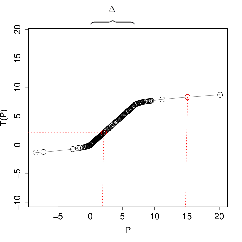
We have found that by defining a metric which encourages the induced cluster boundaries to intersect a compact set, , around the mean of the projected data, the problem of outliers can be mitigated. This is achieved by reducing the distance, relative to the usual Euclidean metric, to points lying outside . Points lying outside , which may be outliers, therefore have increased similarity to all others. We define , where ; and are the mean and standard deviation of the -th component of the projected data; and controls the size of . The modified distance metric, , is defined with respect to a continuously differentiable transformation, , of the projected data,
| (19) | ||||
| (20) | ||||
where is the distance reducing parameter, and and are equalt to and respectively. By construction for any , with strict inequality when either or both .
Figure 6 illustrates the impact of on pairwise distances in the univariate case. As shown, distance increases linearly in the interval , but outside it increases much more slowly, with the rate being determined by . In the limit as approaches zero, all points outside are mapped to the boundary of . As a result distances between points outside and all other points are much smaller after being transformed through , and points which can be characterised as outliers in terms of the original projections, , do not appear as such in terms of .
An illustration of the usefulness of this modified metric is provided in Figure 7. The figure shows two dimensional projections of the 64 dimensional optical recognition of handwritten digits dataset (Bache and Lichman, 2013). The left plots show the true clusters while the right plots show the clustering assignments based on spectral clustering using the normalised Laplacian (Shi and Malik, 2000). Figure 8(a) shows the projection onto the first two principal components, which are also used as initialisation for our method. There are clearly a few points outlying from the remainder of the data, which are separated by the spectral clustering algorithm. Figure 8(b) shows the optimal projection from minimising using the Euclidean metric. The result is that the outlying points have been further separated from the remainder of the data, thereby exacerbating the outlier problem. Finally, Figure 8(c) shows the same result but using the modified metric discussed above, and with . In this case the projection pursuit is able to find a projection which separates two of the true clusters clearly from the remainder.
Appendix B Derivatives
B.1 Evaluating
We first consider the standard Laplacian , and use and to denote the second eigenvalue and corresponding eigenvector. By Eq. (11) we have . Now,
and so,
For the normalised Laplacian, , consider first
We again use and to denote the second eigenvalue and corresponding eigenvector. Using ,
Where in the third step we made use of the fact that
.
Therefore,
B.2 Derivatives of the Approximate Eigenvalue Functions based on Microclusters
In the general case we may consider a set of microclusters with centers and counts . The derivations we provide are valid for , and so apply to the exact formulation of the problem as well. Let . We find it practically convenient to associate the transformation in Eq. (20), which incorporates the set , with the projection of the microclusters rather than with the computation of similarities. Specifically, we now let be the transformed projected microcluster centers, i.e.,
where each is repeated times. The reason for this is that with this formulation the majority of terms in the above sums corresponding to (which are now partial derivatives w.r.t. the elements of , and not as before) are zero. Specifically, with this expression for , and letting be the matrix with columns corresponding to elements in , we have
| (24) |
and similarly for the normalised Laplacian.
In Section 3 we expressed via the chain rule decomposition , which we can now simply restructure as . The compression of to the size non-repeated set, , requires a slight restructuring, as described in Section 5. We begin with the standard Laplacian, letting be the matrix corresponding to , and define and as in Lemma 3. That is, is the diagonal matrix with -th diagonal element equal to and . The derivative of the second eigenvalue of the Laplacian relies on the corresponding eigenvector, . However, this vector is not explicitly available as we only solve the eigen-problem of . Let be the second eigenvector of . As in the proof of Lemma 3 if are such that the -th element of corresponds to the -th microcluster, then . The derivative of with respect to the -th column of , and thus equivalently of the second eigenvalue of the Laplacian is therefore given by
| (25) |
where is given in Eq. (12) and is expressed below. We provide expressions for the case where , as in our implementation, where we have again assumed that the data have been centered, i.e., have zero mean. Then is the matrix with -th row equal to,
if ,
if , and
if . Here is the covariance matrix of the data.
For the normalised Laplacian, the reduced eigenproblem has precisely the same form as the original problem, with the only difference being the introduction of the factors . Specifically, with the derivation in Section 3 we can see that the corresponding derivative is as for the standard Laplacian above, except that the coefficients in Eq. (25) are replaced with , where is the second eigenvalue of the normalised Laplacian, is the corresponding eigenvector and is the degree of the -th element of .
Appendix C Computational Complexity
Here we give a very brief discussion of the computational complexity of the proposed method. At each iteration in the gradient descent, computing the projected data matrix, , requires operations. Computing all pairwise similarities from elements of the -dimensional has computational complexity , and determining both Laplacian matrices, and their associated eigenvalue/vector pairs adds a further computational cost . Each evaluation of the objectives or therefore requires operations. In order to compute the gradients of these objectives, the partial derivatives with respect to each element of the projected data matrix need to be calculated. As we discussed in relation to the derivatives above, the majority of the terms in the sums in Eqs. (13) and (14) are zero, and in fact each partial derivative can be computed in time, and so all such partial derivatives can be computed in time. The matrix derivatives , in (12) can each be computed with operations. Finally, determining the gradients with respect to each column of involves computing the matrix product , where and . This has complexity . The complete gradient calculation therefore requires operations. We have found that the optimality conditions based on directional derivatives and gradient sampling steps are seldom, if ever required, and moreover that these do not constitute the bottleneck in the running time of the method in practice. The complexity of the optimality condition check may be computed along similar lines, and be found to be , where is the multiplicity of the eigenvalue . The gradient sampling is simply times the cost of computing a single gradient. The total complexity of the projection pursuit optimisation depends on the number of iterations in the gradient descent method, where in general this number is bounded for a given accuracy level. For our experiments we use the BFGS (Broyden-Fletcher-Goldfarb-Shanno) algorithm as this has been found to perform well on non-smooth functions (Lewis and Overton, 2013).
Appendix D Proofs
D.1 Proof of Theorem 2
Before proving Theorem 2, we require some supporting theory which we present below. We will use the notation , and for a set and we write, for example, for . Recall that for scaling parameter we define , where is as from before, but with an explicit dependence on the scaling parameter. That is, defines the projection generating the minimal spectral connectivity of for a given value of . We define similarly for the normalised Laplacian.
Recall that we are interested in those hyperplanes which intersect an arbitrary convex set . This is because very often the maximum marging hyperplane will separate only a few points from the remainder, as data tend to be more sparse in the tails of the underlying distribution. To account for the potential for hyperplanes with very large margins lying in the tails of the distribution, we make the additional assumption that the distance reducing parameter, , tends to zero along with .
Lemmas 4 and 5 provide lower bounds on the second eigenvalue of the graph Laplacians of a one dimensional data set in terms of the largest Euclidean separation of adjacent points which lie within the interval , used to represent in the context of a projection of . These lemmas also show how we construct the set . Lemmas 6 and 7 use these results to show that a projection angle leads to lower spectral connectivity than all projections admitting smaller maximal margin hyperplanes intersecting for all pairs sufficiently close to zero.
Lemma 4
Let be a non-increasing, positive function and let . Let be a univariate data set and let for . Suppose that and . Define , where , and . Let . Define to be the Laplacian of the graph with vertices and similarities according to , where is the matrix with -th column equal to . Then , where .
Proof: We can assume that is sorted in increasing order, i.e. , since this does not affect the eigenvalues of . We first show that for all . To this end observe that for .
- •
If then by the definition of and using the above inequality, since is non-increasing. The case is similar.
- •
If then since is the largest margin in .
- •
If none the above hold, then we lose no generality in assuming , since the case , is analogous. We must have and so . If then , a contradiction since and is the largest margin in . Therefore . In all
Now, let be the second eigenvector of . Then and and therefore s.t. . We thus know that there exists s.t. . By (von Luxburg, 2007, Proposition 1), we know that since all consecutive pairs have similarity at least , by above.
Therefore as required.
Lemma 5
Let the conditions of Lemma 4 hold and let be the normalised Laplacian of the graph with vertices and similarities . Then
Proof: The proof is similar to that of Lemma 4, but requires a few simple modifications. Let be the second eigenvector of . Since s.t. . Suppose w/o loss of generality that . Now consider that for all we have and and so for all . Therefore we have . Furthermore, since we have for some . Therefore, . We thus know that s.t. By (von Luxburg, 2007, Proposition 3), we know that
where the bound on is taken from the proof of Lemma 5. Therefore as required.
In the above we have assumed that is contained within the convex hull of the points , however the results of this section can easily be modified to allow for cases where this does not hold. In particular, if an unconstrained large margin hyperplane is sought, then setting to be arbitrarily large allows for this. We have merely stated the results in the most convenient context for our practical implementation.
The set in the above is defined in terms of the one dimensional interval . We define the full dimensional set along the same lines by,
| (26) | ||||
| (27) |
Here we assume that is contained within the convex hull of the -dimensional data set . Notice that since is convex, we have . In what follows we show that as is reduced to zero the optimal projection for spectral partitioning converges to the projection admitting the largest margin hyperplane intersecting . If it is the case that the largest margin hyperplane intersecting also intersects , as is often the case, although this fact will not be known, then it is actually not necessary that tend towards zero. In such cases it only needs to satisfy for the corresponding values of and over all possible projections. In particular, choosing instead of is appropriate for all projections.
Lemma 6
Let and let be non-increasing, positive, and satisfy
for all . Then for any there exists s.t. if and
then .
Proof: Let and . We assume that , since otherwise there is nothing to show. Now, since spectral clustering solves a relaxation of the minimum normalised cut problem we have,
The final inequality holds since for any s.t. and we must have . Now, for any , let . By Lemma 4 we know that , where . Therefore,
Since as , this gives the result.
Lemma 7
Proof: Using a similar approach to that in the proof of Lemma 6, we can arrive at the following.
where the final inequality comes from the fact that for all , and hence vol, and similarly for . The final step in the proof is equivalent to that of Lemma 6, except that is replaced with .
Lemmas 6 and 7 show almost immediately that the margin admitted by the optimal projection for spectral bi-partitioning converges to the largest margin through as goes to zero. Theorem 2, which we are now in
a position to prove, shows the stronger result that the optimal projection itself converges to the projection admitting the largest margin.
Proof of Theorem 2:
Take any . Pavlidis et al. (2016) have shown that s.t. for , margin margin. By Lemma 6 we know , s.t. if then s.t. margin margin, since is optimal for . Thus, by above, . But for any . Since was arbitrary, we therefore have as . The proof for is analogous.
D.2 Proof of Lemma 3
The proof of Lemma 3 uses the following result from matrix perturbation theory.
Theorem 8 (Ye (2009))
Let and be two symmetric positive semidefinite diagonally dominant matrices, and let and be their respective eigenvalues. If, for some , , and where , and similarly for , then
An inspection of the proof of Theorem 8 reveals that
is necessary only to ensure that the signs of are the
same as those of . In the case of Laplacian matrices this
equivalence of signs holds by design, and so in this context the requirement
that can be relaxed.
Now, for brevity we drop the notational dependence on . Let , where each is repeated times, and let be the corresponding matrix of repeated projected centroids. Let be the Laplacian of the graph with vertices and edges given by . We begin by showing that . Take , then,
and so is positive semi-definite. In addition, it is straightforward to verify that , and hence is the smallest eigenvalue of with eigenvector . Now, let be the second eigenvector of . Then for pairs of indices aligned with the same in . Define s.t. where index is aligned with in . Then where index is aligned with in for each . Therefore and hence since is the smallest eigenvector of and so . Similarly . Thus and and so is a candidate for the second eigenvector of . In addition it is straightforward to show that . Now, suppose by way of contradiction that with s.t. . Then let where each is repeated times. Then , and , a contradiction since is the second eigenvector of .
Now, let be such that and . We temporarily drop the notational dependence on . Then,
since contracts distances and and are the radii of and . Since is non-increasing we therefore have,
| and | |||
Therefore
Now, we lose no generality by assume that is ordered such that for each the elements of cluster are aligned with in , since this does not affect the eigenvalues of the Laplacian of , . By the design of the Laplacian matrix the “” of Theorem 8 are exactly zero. For off diagonal terms with corresponding as above, consider
Theorem 8 thus gives the result.
References
- Bach and Jordan (2006) Bach, F.R., Jordan, M.I.: Learning spectral clustering, with application to speech separation. Journal of Machine Learning Research 7, 1963–2001 (2006)
- Bache and Lichman (2013)
Bache, K., Lichman, M.: UCI machine learning repository (2013).
http://archive.ics.uci.edu/ml - Boumal et al. (2014)
Boumal, N., Mishra, B., Absil, P.A., Sepulchre, R.: Manopt, a matlab toolbox
for optimization on manifolds.
Journal of Machine Learning Research 15, 1455–1459 (2014).
http://jmlr.org/papers/v15/boumal14a.html - Burke et al. (2006) Burke, J.V., Lewis, A.S., Overton, M.L.: A robust gradient sampling algorithm for nonsmooth, nonconvex optimization. SIAM Journal on Optimization 15(3), 751–779 (2006)
- Chi et al. (2009)
Chi, Y., Song, X., Zhou, D., Hino, K., Tseng, B.L.: On evolutionary spectral
clustering.
ACM Transactions on Knowledge Discovery from Data 3(4),
17:1–17:30 (2009).
doi: 10.1145/1631162.1631165.
http://doi.acm.org/10.1145/1631162.1631165 - Edelman et al. (1998) Edelman, A., Arias, T., Smith, S.T.: The geometry of algorithms with orthogonality constraints. SIAM Journal on Matrix Analysis and Applications 20(2), 303–353 (1998)
- Fan (1949) Fan, K.: On a theorem of weyl concerning eigenvalues of linear transformations i. Proceedings of the National Academy of Sciences of the United States of America 35(11), 652 (1949)
- Hagen and Kahng (1992) Hagen, L., Kahng, A.B.: New spectral methods for ratio cut partitioning and clustering. IEEE transactions on computer-aided design of integrated circuits and systems 11(9), 1074–1085 (1992)
- Hartigan and Hartigan (1985) Hartigan, J.A., Hartigan, P.M.: The dip test of unimodality. The Annals of Statistics 13(1), 70–84 (1985)
- Hastie et al. (2009) Hastie, T., Tibshirani, R., Friedman, J.: The Elements of Statistical Learning: Data Mining, Inference, and Prediction. Springer Texts in Statistics. Springer, 2 ed. (2009)
- Hofmeyr and Pavlidis (2015) Hofmeyr, D., Pavlidis, N.: Maximum clusterability divisive clustering. In: Computational Intelligence, 2015 IEEE Symposium Series on, pp. 780–786. IEEE (2015)
- Joachims (1999) Joachims, T.: Transductive inference for text classification using support vector machines. In: Proceedings of International Conference on Machine Learning (ICML), vol. 99, pp. 200–209. Bled, Slowenien (1999)
- Kaiser (1960) Kaiser, H.F.: The application of electronic computers to factor analysis. Educational and psychological measurement 20(1), 141–151 (1960)
- Krause and Liebscher (2005) Krause, A., Liebscher, V.: Multimodal projection pursuit using the dip statistic. Preprint-Reihe Mathematik 13 (2005)
- Lewis and Overton (2013) Lewis, A., Overton, M.: Nonsmooth optimization via quasi-Newton methods. Mathematical Programming 141, 135–163 (2013)
- Lewis and Overton (1996) Lewis, A.S., Overton, M.L.: Eigenvalue optimization. Acta numerica 5, 149–190 (1996)
- Magnus (1985) Magnus, J.R.: On differentiating eigenvalues and eigenvectors. Econometric Theory 1(02), 179–191 (1985)
- Ng et al. (2002) Ng, A., Jordan, M.I., Weiss, Y.: On spectral clustering: analysis and an algorithm. In: Dietterich, T., Becker, S., Ghahramani, Z. (eds.) Advances in Neural Information Processing Systems 14, pp. 849 –856. MIT Press, Cambridge (2002)
- Ning et al. (2010) Ning, H., Xu, W., Chi, Y., Gong, Y., Huang, T.S.: Incremental spectral clustering by efficiently updating the eigen-system. Pattern Recognition 43(1), 113–127 (2010). doi: http://dx.doi.org/10.1016/j.patcog.2009.06.001
- Niu et al. (2011) Niu, D., Dy, J.G., Jordan, M.I.: Dimensionality reduction for spectral clustering. In: International Conference on Artificial Intelligence and Statistics, pp. 552–560 (2011)
- Nocedal and Wright (2006) Nocedal, J., Wright, S.: Numerical optimization. Springer Science & Business Media (2006)
- Overton and Womersley (1993) Overton, M.L., Womersley, R.S.: Optimality conditions and duality theory for minimizing sums of the largest eigenvalues of symmetric matrices. Mathematical Programming 62(1-3), 321–357 (1993)
- Pavlidis et al. (2016) Pavlidis, N., Hofmeyr, D., Tasoulis, S.: Minimum density hyperplanes. arXiv preprint arXiv:1507.04201v2 (2016)
- Peña and Prieto (2001) Peña, D., Prieto, F.J.: Cluster identification using projections. Journal of the American Statistical Association (2001)
- Polak (1987) Polak, E.: On the mathematical foundations of nondifferentiable optimization in engineering design. SIAM Review 29(1), 21–89 (1987). doi: 10.1137/1029002
- Rahimi and Recht (2004) Rahimi, A., Recht, B.: Clustering with normalized cuts is clustering with a hyperplane. Statistical Learning in Computer Vision 56 (2004)
- Schur (1911) Schur, J.: Bemerkungen zur theorie der beschränkten bilinearformen mit unendlich vielen veränderlichen. Journal für die reine und Angewandte Mathematik 140, 1–28 (1911)
- Shi and Malik (2000) Shi, J., Malik, J.: Normalized cuts and image segmentation. Pattern Analysis and Machine Intelligence, IEEE Transactions on 22(8), 888–905 (2000)
- Strehl and Ghosh (2002) Strehl, A., Ghosh, J.: Cluster ensembles—a knowledge reuse framework for combining multiple partitions. Journal of machine learning research 3(Dec), 583–617 (2002)
- Tong and Koller (2000) Tong, S., Koller, D.: Restricted bayes optimal classifiers. In: AAAI/IAAI, pp. 658–664 (2000)
- Vapnik and Kotz (1982) Vapnik, V.N., Kotz, S.: Estimation of dependences based on empirical data, vol. 40. Springer-verlag New York (1982)
- von Luxburg (2007) von Luxburg, U.: A tutorial on spectral clustering. Statistics and Computing 17(4), 395–416 (2007). doi: 10.1007/s11222-007-9033-z
- Wagner and Wagner (1993) Wagner, D., Wagner, F.: Between min cut and graph bisection. Springer (1993)
- Weiss (1999) Weiss, Y.: Segmentation using eigenvectors: a unifying view. In: Proceedings of the 7th IEEE International Conference on Computer Vision, vol. 2, pp. 975–982 (1999)
- Weyl (1912) Weyl, H.: Das asymptotische verteilungsgesetz der eigenwerte linearer partieller differentialgleichungen (mit einer anwendung auf die theorie der hohlraumstrahlung). Mathematische Annalen 71(4), 441–479 (1912)
- Wolfe (1972) Wolfe, P.: On the convergence of gradient methods under constraint. IBM Journal of Research and Development 16(4), 407–411 (1972)
- Xu et al. (2004) Xu, L., Neufeld, J., Larson, B., Schuurmans, D.: Maximum margin clustering. In: Advances in neural information processing systems, pp. 1537–1544 (2004)
- Yan et al. (2009) Yan, D., Huang, L., Jordan, M.I.: Fast approximate spectral clustering. In: Proceedings of the 15th ACM SIGKDD international conference on Knowledge discovery and data mining, pp. 907–916. ACM (2009)
- Ye (2009) Ye, Q.: Relative perturbation bounds for eigenvalues of symmetric positive definite diagonally dominant matrices. SIAM Journal on Matrix Analysis and Applications 31(1), 11–17 (2009)
- Zelnik-Manor and Perona (2004) Zelnik-Manor, L., Perona, P.: Self-tuning spectral clustering. In: Advances in neural information processing systems, pp. 1601–1608 (2004)
- Zhang (2001) Zhang, B. Dependence of clustering algorithm performance on clustered-ness of data. Tech. rep., Technical Report, 20010417. Hewlett-Packard Labs (2001)
- Zhang et al. (2009) Zhang, K., Tsang, I.W., Kwok, J.T.: Maximum margin clustering made practical. Neural Networks, IEEE Transactions on 20(4), 583–596 (2009)
- Zhang et al. (1996) Zhang, T., Ramakrishnan, R., Livny, M.: Birch: an efficient data clustering method for very large databases. In: ACM SIGMOD Record, vol. 25, pp. 103–114. ACM (1996)
- Zhao and Karypis (2004) Zhao, Y., Karypis, G.: Empirical and theoretical comparisons of selected criterion functions for document clustering. Machine Learning 55(3), 311–331 (2004)