Heavy quark potential from QCD-related effective coupling
Abstract
We implement our past investigations in the quark-antiquark interaction through a non-perturbative running coupling defined in terms of a gluon mass function, similar to that used in some Schwinger-Dyson approaches. This coupling leads to a quark-antiquark potential, which satisfies not only asymptotic freedom but also describes linear confinement correctly. From this potential, we calculate the bottomonium and charmonium spectra below the first open flavor meson-meson thresholds and show that for a small range of values of the free parameter determining the gluon mass function an excellent agreement with data is attained.
pacs
12.38.Aw, 12.39.Pn, 12.38.Lg, 14.40.PqI Introduction
The use of perturbation theory in quantum chromodynamics (QCD) [1] provides a useful tool to study high energy processes as confirmed by the accurate description of deep inelastic lepton-nucleon and nucleon-nucleon collision processes [2, 3, 4].
Asymptotic freedom [5, 6] is the fundamental property of QCD that justifies the use of perturbation methods to describe the interaction among the constituents at high momentum transfers (short distances).
In order to describe low energy (large distance) physics, for example the hadron spectrum, perturbation theory cannot be used. The reason being that the interaction among the constituents is dominated by another fundamental property of QCD, the confinement of quarks and gluons [7], which is highly non-perturbative. Efforts have been made and techniques developed to study this low momentum transfer regime, e.g. lattice QCD [9, 8], phenomenological quark potential models [10, 11, 12], studies on the nontrivial vacuum [13], effective theories [14], dispersive extensions of the beta function [15, 16], and the solution of the Schwinger-Dyson equations [17, 18]. Another development which has led to very succesful results in the study of the spectrum and the behavior of the strong coupling in the infrared (IR) is AdS/CFT [19, 20].
The resolution of Schwinger-Dyson equations (SDE) leads to the freezing of the QCD running coupling (effective charge) in the infrared which can be conveniently understood as a dynamical generation of a gluon mass function, giving rise to a momentum dependence which is free from IR divergences [17, 18, 21, 22, 23] . It was shown that the interquark static potential for heavy mesons described by a massive one gluon exchange interaction obtained from the propagator of the truncated Schwinger-Dyson equations does not reproduce the expected Cornell potential [24]. This was attributed to the lack of a mechanisms for confinement [24] by explicit comparison with lattice QCD calculations [25].
To solve this problem an ad hoc effective mechanism was proposed based on a singular nonperturbative coupling [26], which generates a Gribov singularity in the potential while keeping the propagator infrared finite. We show here that the proposal leads to a potential with linear confinement and the correct asymptotic behavior of QCD. The resulting potential is Cornell like for intermediate distances ( fm) and for a small range of values of the free parameter determining the gluon mass function it provides a good spectral description of heavy quarkonia.
Other authors have also used non-perturbative effective couplings which reproduce asymptotic freedom in the UV and have behavior in the IR to study the spectrum and other physical observables [27, 28, 29, 30, 31, 32]. These couplings have been justified from QCD under certain requirements [33, 34, 35]. However, it must be noted that many succesful phenomenological studies of the IR coupling point to a finite value [36].
The contents of this paper are organized as follows. In Section II we establish the prescription to get the static quark-antiquark potential from the running coupling. A possibility to generate a linear confining potential is through a strong Gribov singularity for small momenta. We propose a functional form resulting from a modification of the Schwinger-Dyson solution for the coupling, which has the desired singularity structure at small momenta and satisfies asymptotic freedom at large momenta. The presence of the singularity requires, in order to get the potential, a regularization scheme which is described in detail in Section III. Then, in Section IV, the results obtained are presented. The potential is compared to the Cornell one. The calculated heavy quarkonia masses are compared with data and with the ones resulting from “equivalent” Cornell potentials. Finally, in Section V, the main conclusions of this work are summarized.
II Quark-Antiquark Potential from the non-perturbative running coupling
The history of the theoretical description of the quark-antiquark potential and its relation to QCD has been motivated by the tremendous phenomenological success of the Cornell potential [10, 11]
| (1) |
where , the Coulomb strength, and , the string tension, are constants to be fitted from data. It is amazing that this simple potential reproduces quite accurately the experimental heavy quark meson spectra below the open flavor meson-meson threshold energies (see Section IV).
Two limits characterize this potential. The short distance limit which satisfies asymptotic freedom, and the long distance limit which describes the IR behavior, i.e. confinement of heavy static sources.
In general, a quark-antiquark potential in configuration space, reads (note that the angular variables have been integrated)
| (2) |
where is the potential in momentum space.
By assuming one gluon exchange dominance, can be derived from QCD as
| (3) |
with and standing for the running coupling and the gluon propagator respectively.
It is now well established from lattice QCD, and confirmed by Schwinger-Dyson calculations, that the finite character of the propagator (at ) reads [17, 18]
| (4) |
where is an effective gluon mass (see below). Other points of view to parametrize the gluon propagator have been developed, like flux tubes [12] and effective potentials [20], in which the connection to the concept of massive gluon exchange is not currently known.
Regarding the coupling, a truncated solution of a gauge invariant subset of the Schwinger-Dyson equations for QCD gives rise to a functional form showing a freezing in the IR which can be cast as [18] :
| (5) |
where is the first -function coefficient for QCD, being the number of active quarks, is the scale parameter in QCD and is a gluon mass given by [37]
| (6) |
with , and constants. Other parametrizations for both coupling and gluon mass can be found in ref. [36]. The coupling (5) is to first order the one proposed in [21] obtained from the gluon propagator using the pinch technique. Note that the dynamical gluon mass varies with the number of flavors () [22, 23] and therefore is determined by the initial and the QCD scale .
The combination (3), (4), (5) and (6) is renormalization group invariant since the ghost contribution has been incorporated into the definition of the coupling [24]. Therefore one can construct a potential. The result is a non linearly rising potential [24] contrary to the expectation from the quenched approximation followed to derive the propagator and the coupling. Actually a linearly rising Cornell-like behavior has been obtained in quenched lattice QCD [9, 25]. One possible reason for this anomaly might be that confinement is more than a one gluon exchange effect. An alternative possibility, suggested in reference [26], is that the Schwinger-Dyson coupling contains the physics at intermediate and large but it lacks some vertex corrections at low . We shall examine this alternative next.
For this purpose we realize that in order to lead to linear confinement the mass singularity of the propagator must be eliminated and instead a Gribov singularity should appear. An easy way to do this from (5) is through the modified coupling
| (7) |
so that the factor cancels the singularity of the propagator whereas the factor gives rise altogether with to a Gribov singularity. In this way the low behavior of has been corrected as required while the intermediate and long distance dependencies are preserved since is a quickly decreasing function with When our potential becomes in the IR limit, , that of Richardson [27], signaling that it is defined in the scheme. Moreover, reproduces in the asymptotic limit the well known one-loop perturbative QCD result
Additional terms of the order , where , have to be added to this result but hey are negiglible and arise from the IR behavior [38].
In order to check whether this modified coupling proposal is physically meaningful or not we shall study, from the potential deriving from it, heavy quarkonia, using as a criterion of meaningfulness the accurate description of the spectra. More precisely, we shall choose for the evolution mass parameters and their estimated values in the Schwinger Dyson context [37]
while leaving () as the free parameter of the potential. Then, an accurate spectral description for a reasonable value of might be an indication that the proposed coupling parametrizes efficiently and conveniently the phenomenology.
It must be stressed at this point that we have incorporated the Gribov singularity guided by lattice QCD and simplicity and in so doing we have departed from the SDE approach. Nevertheless the effective way of introducing the coupling mantains the behavior of the SDE result for large and intermediate energies and therefore a good fit of the spectrum is strong support of the SDE calculation.
III Regularization procedure
| (8) |
The integral in (8) is divergent since the integrand behaves as at the origin . To extract its physical content we have to regularize it. To understand how the regularization procedure works let us consider the simpler case of the potential (with the same singular behavior at the origin)
where is an dimensionless constant. Its Fourier transform, from (2), is given by
By introducing a regulator we can rewrite it as
so that the integral can be solved analytically in the complex plane giving
The divergent term does not depend on . As the potential is defined up to an arbitrary constant we may simply remove such spurious divergence from the potential. To do this in a more systematic way, let us realize that the divergent term comes out from the behavior of the integrand at . Then, by making an expansion of the integrand around ,
we can easily identify the first term as causing the divergence of the integral at . Indeed, if we integrate this term with the same regularization procedure we get
Therefore we can redefine the potential by subtracting this non physical divergence as
Back to (8) it is more convenient to regularize it through a cutoff in the form
To subtract the spurious divergence we expand the integrand around
and keep only the terms giving rise after integration to a singular behavior at (they correspond, for , to the explicitly written ones). By integrating these terms with the chosen cutoff regularization we get
so that the physical potential reads
| (9) |
which is evaluated numerically.
IV Results
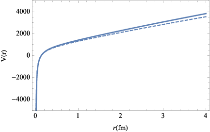
In order to fix , the only free parameter of the potential, we require (9) to provide a reasonable description of the heavy quarkonia (bottomonium and charmonium) spectra. As will be justified later on, for bottomonium, one has to use and for charmonium . To calculate the spectrum we solve the Schrödinger equation. For any value of , we choose the quark masses, and , to get the best spectral fit. In this regard, as (9) represents a quenched potential we restrict the comparison with data to energies below the corresponding open flavor meson-meson thresholds.
It turns out that only for a quite restricted range of values of ( MeV) a good spectral description for bottomonium and charmonium is obtained. The corresponding potentials for MeV are shown in Fig. 1.
As can be seen, the potential (9) shows a soft flavor dependence in the slope for intermediate and large distances. However, if we use also for bottomonium the calculated spectral masses will only change slightly.
In Tables 1 and 2 we list the calculated masses for bottomonium and charmonium for MeV as compared to data. To denote the states we use the spectroscopic notation in terms of the radial, and orbital angular momentum, quantum numbers of the quark-antiquark system. As we are dealing with a spin-independent potential we compare as usual the calculated wave state masses with spin-triplet data, the wave state masses with the centroids obtained from data and the wave states with the few existing experimental candidates.
A very good spectral description is attained. Note that the only significant difference ( MeV) between the calculated masses and data is for the charmonium state and it may be explained through configuration mixing with the one.
For further comparison the spectra from “equivalent” Cornell potentials have also been quoted. This equivalence is based on the observation that for intermediate distances ( fm) the potentials (9) can be very well approximated by the Cornell types
| (10) |
with
| (11) | ||||
and
| (12) |
with
| (13) | ||||
where the fitted Coulomb strengths are in agreement with the values derived from QCD from the hyperfine splitting of states in bottomonium [40] and from the fine structure splitting of states in charmonium [41].
As a matter of fact, in the mentioned region, they can not be distinguished from those in Fig. 1. However, below and above this region they become different as shown in Figs. 2 and 3 for bottomonium.
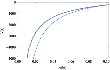
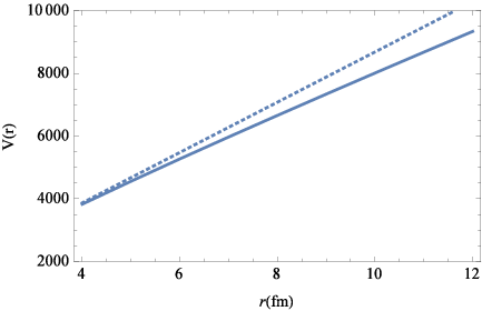
These differences have not much effect on the calculated masses, as can be seen in Tables 1 and 2. However, in order to get a more accurate fit to the spectra from a Cornell potential the string tensions have to be slightly increased with respect to those of (10) and (12).
It is interesting to check a posteriori our initial assumption about the number of active quarks ( for charmonium and for bottomonium). The momentum determines the active number of flavors in the coupling, thus if
where is the three-momentum of the quark (charm or bottom) in the center-of-mass system, then is to be used in the coupling. This can be conveniently rewritten as
where is the relative quark-antiquark velocity. By using the values calculated from the wave functions, and we can see that in charmonium , for strangeness, and therefore , while in bottomonium, and therefore .
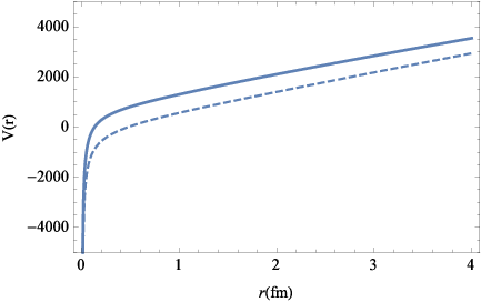
It is illustrative to compare the potential (9) fitting the charmonium spectrum (with MeV, see Table 2) with the potential of Richardson [27] obtained from (3) with and
| (14) |
This comparison is shown in Fig. 4. Although generated from different approaches, both potentials give a similar quality fits to the spectrum. It must be recalled that both potentials are defined in the scheme. The value of required by equation (9) ( MeV) is in better agreement with QCD than Richardson’s ( MeV) [27], since in the scheme, (4 Loops, ) MeV and (4 Loops, ) MeV [42, 43, 44].
V Conclusions
This work has been motivated by previous studies aiming at describing the phenomenological successful potentials from QCD [24, 26]. Our aim here has been to describe the heavy quark spectra from a potential derivable from non-perturbative QCD studies. Our research has led to a simple description of linear confinement in quenched QCD in terms of a gluon mass function describing the non-perturbative coupling.
There are several issues which have arisen in our investigation that merit attention and which we next recall.
Confinement can be described by a one-gluon-exchange picture if some of the long-distance physics is folded in an effectively generated gluon mass. In that context asymptotic freedom of the coupling and phenomenology require that the gluon mass function goes rapidly to zero, faster than . This result is in complete agreement with lattice QCD and the SDE solutions.
In that context, a Gribov type singularity is the least requirement for linear confinement. This IR singular behavior is an ad hoc assumption, which many phenomenological studies of the IR coupling do not support [36], and implies that the SDE formulation of the gluon mass function must be restricted to . If , linear confinement will soften to a Yukawa type behavior. In the present non-relativistic dynamical scheme this type of potentials are non confining, however this is not so in other formulations [20].
A main result of our analysis is that we are led to Cornell type potentials in the region relevant to describe the spectra ( fm). In this way we support the phenomenological success associated with Cornell type potential as a consequence of QCD.
Our fit of the spectra is excellent. Note that we have used only one free parameter, which comes out at a very reasonable value ( MeV). Moreover, we justify the slight difference between the bottomonium and charmonium potentials in terms of the number of flavors entering the coupling.
Therefore we have shown that by incorporating the infrared Gribov singularity in a manner that respects the behavior of the massive SDE coupling with fixed parameters at large we obtain an excellent potential capable of reproducing the heavy hadron spectrum with only one parameter, , which moreover comes at a wishful value GeV close to the value determined from other phenomenology in the scheme. Moreover, the flavor dependence of the SDE coupling controls the flavor dependence of the potential. While our potential is very close to the Cornell potential in the physical range it differs from it outside the range and has a perfect asymptotic QCD behavior. Moreover this coupling not only can be used to explain the spectrum but can be used in many other processes where we are dealing with large to moderate energies.
We conclude by stating that we have found an explanation for the phenomenological successful potentials in terms of a non-perturbative effective mechanism describing the strong coupling. This mechanism is defined by means of a gluon mass function with properties closely related to lattice QCD and SDE studies to which we have incorporated in a gentle way the Gribov singularity. We have supported the successful Cornell type potentials as arising from specific mechanisms in non-perturbative QCD.
Acknowledgements.
We acknowledge useful comments by G. Cvetič. This work has been supported in part by MINECO (Spain) Grants. Nos. FPA2013-47443-C2-1-P and FPA2014-53631-C2-1-P, GVA-PROMETEOII/2014/066, SEV-2014-0398 and CA also by CONICYT “Becas Chile” Grant No.74150052 .References
- [1] H. Fritzsch, M. Gell-Mann and H. Leutwyler, Phys. Lett. B 47, 365 (1973).
- [2] Y. L. Dokshitzer, Sov. Phys. JETP 46 (1977) 641 [Zh. Eksp. Teor. Fiz. 73 (1977) 1216].
- [3] V. N. Gribov and L. N. Lipatov, Sov. J. Nucl. Phys. 15 (1972) 438 [Yad. Fiz. 15 (1972) 781].
- [4] G. Altarelli and G. Parisi, Nucl. Phys. B 126 (1977) 298.
- [5] D. J. Gross and F. Wilczek, Phys. Rev. Lett. 30, 1343 (1973).
- [6] H. D. Politzer, Phys. Rev. Lett. 30, 1346 (1973).
- [7] K. G. Wilson, Phys. Rev. D 10 (1974) 2445.
- [8] P. Hagler, Prog. Theor. Phys. Suppl. 187 (2011) 221.
- [9] G. S. Bali, Phys. Rept. 343, 1 (2001) [hep-ph/0001312].
- [10] E. Eichten, K. Gottfried, T. Kinoshita, K. D. Lane and T. M. Yan, Phys. Rev. D 17, 3090 (1978) [Phys. Rev. D 21, 313 (1980)].
- [11] C. Quigg and J. L. Rosner, Phys. Rept. 56, 167 (1979).
- [12] S. Godfrey and N. Isgur, Phys. Rev. D 32, 189 (1985).
- [13] N. I. Kochelev, Sov. J. Nucl. Phys. 41 (1985) 291 [Yad. Fiz. 41 (1985) 456].
- [14] N. Brambilla and A. Vairo, In *Newport News 1998, Strong interactions at low and intermediate energies* 151-220 [hep-ph/9904330].
- [15] A. V. Nesterenko, Phys. Rev. D 64 (2001) 116009 [hep-ph/0102124].
- [16] A. V. Nesterenko, Int. J. Mod. Phys. A 18 (2003) 5475 [hep-ph/0308288].
- [17] J. M. Cornwall, Phys. Rev. D 26, 1453 (1982).
- [18] A. C. Aguilar and J. Papavassiliou, JHEP 0612, 012 (2006).
- [19] J. Erlich, E. Katz, D. T. Son and M. A. Stephanov, Phys. Rev. Lett. 95 (2005) 261602 doi:10.1103/PhysRevLett.95.261602 [hep-ph/0501128].
- [20] S. J. Brodsky, G. F. de Teramond, H. G. Dosch and J. Erlich, Phys. Rept. 584 (2015) 1 doi:10.1016/j.physrep.2015.05.001 [arXiv:1407.8131 [hep-ph]].
- [21] A. C. Aguilar, D. Binosi, J. Papavassiliou and J. Rodriguez-Quintero, Phys. Rev. D 80 (2009) 085018 [arXiv:0906.2633 [hep-ph]].
- [22] A. Ayala, A. Bashir, D. Binosi, M. Cristoforetti and J. Rodriguez-Quintero, Phys. Rev. D 86 (2012) 074512 doi:10.1103/PhysRevD.86.074512 [arXiv:1208.0795 [hep-ph]].
- [23] A. C. Aguilar, D. Binosi and J. Papavassiliou, Phys. Rev. D 88 (2013) 074010 doi:10.1103/PhysRevD.88.074010 [arXiv:1304.5936 [hep-ph]].
- [24] P. Gonzalez, V. Mathieu and V. Vento, Phys. Rev. D 84, 114008 (2011) [arXiv:1108.2347 [hep-ph]].
- [25] J. Greensite, S. Olejnik, Phys. Rev. D67 (2003) 094503. [hep-lat/0302018].
- [26] V. Vento, Eur. Phys. J. A 49 (2013) 71 [arXiv:1205.2002 [hep-ph]].
- [27] J. L. Richardson, Phys. Lett. B 82, 272 (1979).
- [28] W. Buchmuller and S. H. H. Tye, Phys. Rev. D 24 (1981) 132.
- [29] A. V. Nesterenko, Phys. Rev. D 62, 094028 (2000) [hep-ph/9912351].
- [30] L. N. Epele, H. Fanchiotti, C. A. Garcia Canal and M. Marucho, Phys. Lett. B 523 (2001) 102 [hep-ph/0103186].
- [31] E. G. S. Luna, A. L. dos Santos and A. A. Natale, Phys. Lett. B 698 (2011) 52 [arXiv:1012.4443 [hep-ph]].
- [32] J. D. Gomez and A. A. Natale, arXiv:1509.04798 [hep-ph].
- [33] V. N. Gribov, Eur. Phys. J. C 10 (1999) 91 [hep-ph/9902279].
- [34] Y. A. Simonov, hep-ph/9911237.
- [35] F. J. Yndurain, Nucl. Phys. Proc. Suppl. 93 (2001) 196 [hep-ph/0008007].
- [36] A. Deur, S. J. Brodsky and G. F. de Teramond, Prog. Part. Nucl. Phys. 90 (2016) 1 doi:10.1016/j.ppnp.2016.04.003 [arXiv:1604.08082 [hep-ph]].
- [37] A. C. Aguilar, D. Binosi and J. Papavassiliou, Phys. Rev. D 89, 085032 (2014) [arXiv:1401.3631 [hep-ph]].
- [38] M. A. Shifman, A. I. Vainshtein and V. I. Zakharov, Nucl. Phys. B 147, 385 (1979).
- [39] K. A. Olive et al. [Particle Data Group (PDG)], Chin. Phys. C 38, 090001 (2014).
- [40] S. Titard and F. J. Ynduráin, Phys. Lett. B 351, 541 (1995); Phys. Rev. D 51, 6348 (1995).
- [41] A. M. Badalian and V. L. Morgunov, Phys. Rev. D 60, 116008 (1999).
- [42] F. J. Yndurain, The theory of quark and gluon interactions, Berlin, Germany: Springer (2006).
- [43] A. L. Kataev, G. Parente and A. V. Sidorov, Phys. Part. Nucl. 34 (2003) 20 [Fiz. Elem. Chast. Atom. Yadra 34 (2003) 43] [Phys. Part. Nucl. 38 (2007) 6, 827] [hep-ph/0106221].
- [44] A. L. Kataev and V. S. Molokoedov, Phys. Rev. D 92, 054008 [arXiv:1507.03547 [hep-ph]].