跳到论文正文
W Papers独立论文阅读器 arXiv:1509.01348 论文正文 计算阅读时间 · 0%
引用这篇论文根据当前论文元数据生成,正式投稿前建议核对。


License: arXiv.org perpetual non-exclusive license
arXiv:1509.01348v1 [math.PR] 04 Sep 2015

Computation of sensitivities for the invariant measure of a parameter dependent diffusion

Roland Assaraf Note: Laboratoire de Chimie Théorique, CNRS-UMR 7616 et Université Pierre et Marie Curie, 75252 Paris Cedex, France, assaraf@lct.jussieu.fr    Benjamin Jourdain Note: Université Paris-Est, CERMICS (ENPC), INRIA, F-77455 Marne-la-Vallée, France, jourdain@cermics.enpc.fr    Tony Lelièvre Note: Université Paris-Est, CERMICS (ENPC), INRIA, F-77455 Marne-la-Vallée, France, lelievre@cermics.enpc.fr    Raphaël Roux Note: Laboratoire de Probabilités et Modèles Aléatoires, UMR 7599, UPMC, Case 188, 4 pl. Jussieu, F-75252 Paris Cedex 5, France, raphael.roux@upmc.fr
Abstract

We consider the solution to a stochastic differential equation with a drift function which depends smoothly on some real parameter λ\lambda, and admitting a unique invariant measure for any value of λ\lambda around λ=0\lambda=0. Our aim is to compute the derivative with respect to λ\lambda of averages with respect to the invariant measure, at λ=0\lambda=0. We analyze a numerical method which consists in simulating the process at λ=0\lambda=0 together with its derivative with respect to λ\lambda on long time horizon. We give sufficient conditions implying uniform-in-time square integrability of this derivative. This allows in particular to compute efficiently the derivative with respect to λ\lambda of the mean of an observable through Monte Carlo simulations.

Keywords: Stochastic differential equations, invariant measure, variance reduction, Feynman-Kac formulae.

1 Introduction

We are interested in methods to compute the response of a Brownian dynamics to an infinitesimal change of a parameter λ∈ℝ\lambda\in\mathbb{R}. More precisely, we consider the dynamics in ℝd\mathbb{R}^{d}:

{d​Xtλ=Fλ​(Xtλ)​d​t+2​d​Wt,X0λ=X0,\left\{\begin{aligned} \mathrm{d}X_{t}^{\lambda}&=F_{\lambda}(X_{t}^{\lambda})\mathrm{d}t+\sqrt{2}\mathrm{d}W_{t},\\ X_{0}^{\lambda}&=X_{0},\end{aligned}\right. (1)

for λ∈ℝ\lambda\in\mathbb{R} close to 00, where (Wt)t≥0(W_{t})_{t\geq 0} is a standard dd-dimensional Brownian motion independent of X0∈ℝdX_{0}\in\mathbb{R}^{d}. Note that neither the initial condition X0X_{0} nor the Brownian motion depend on λ\lambda. The family of vector fields Fλ:ℝd→ℝdF_{\lambda}:\mathbb{R}^{d}\to\mathbb{R}^{d} is indexed by a real parameter λ\lambda. We assume that when λ=0\lambda=0, the vector field derives from some potential energy V:ℝd→ℝV:\mathbb{R}^{d}\to\mathbb{R}, namely

F0=−∇V,F_{0}=-\nabla V,

where ∇\nabla denotes the gradient operator with respect to the space variables. For λ\lambda close to zero, one can think of (Xtλ)t≥0(X_{t}^{\lambda})_{t\geq 0} as a physical system undergoing a potential energy VV to which one applies an external force λ​∂λ0Fλ\lambda\partial_{\lambda}^{0}F_{\lambda}. Here and in all the following, the notation ∂λ0\partial_{\lambda}^{0} denotes the derivative with respect to λ\lambda computed at λ=0\lambda=0.

Concerning the potential VV, we assume that the following assumption holds.

Assumption (Pot).

The function VV satisfies the following assumptions:

  1. (i)

    V:ℝd→ℝV:\mathbb{R}^{d}\to\mathbb{R} is a 𝒞2\mathcal{C}^{2} function such that x↦∇2V​(x)x\mapsto\nabla^{2}V(x) is locally Lipschitz.

  2. (ii)

    ∫ℝde−V⁡(x)​𝑑x=1\displaystyle{\int_{\mathbb{R}^{d}}e^{-V(x)}\mathrm{d}x=1} and ∫ℝd|∇V|2​(x)​e−V⁡(x)​𝑑x<∞\displaystyle{\int_{\mathbb{R}^{d}}|\nabla V|^{2}(x)e^{-V(x)}\mathrm{d}x<\infty}.

  3. (iii)

    Pathwise existence and uniqueness hold for the process (Xt0)t≥0(X_{t}^{0})_{t\geq 0}.

Since ∇V\nabla V is assumed to be locally Lipschitz, pathwise uniqueness is automatically ensured. Pathwise existence is ensured for instance as soon as there exists a finite constant CC such that for all x∈ℝd,x\in\mathbb{R}^{d}, ∇V​(x)⋅x≤C⁡(1+|x|2)\nabla V(x)\cdot x\leq C(1+|x|^{2}).

At λ=0\lambda=0, the dynamics (1) is of the following gradient form

d​Xt0=−∇V​(Xt0)​d​t+2​d​Wt.\mathrm{d}X_{t}^{0}=-\nabla V(X_{t}^{0})\mathrm{d}t+\sqrt{2}\mathrm{d}W_{t}. (2)

Under the above assumptions, it can be checked that e−V⁡(x)​d​xe^{-V(x)}\mathrm{d}x is the unique invariant probability measure (see Lemma 18 below) denoted in the following:

d​π0=e−V⁡(x)​d​x.\mathrm{d}\pi_{0}=e^{-V(x)}\mathrm{d}x.

Then, from classical results in ergodic theory, for any ff in 𝕃1​(π0)\mathbb{L}^{1}(\pi_{0}), almost surely,

limt→∞1t​∫0tf⁡(Xs0)​𝑑s=∫ℝdf​d​π0.\lim_{t\to\infty}\frac{1}{t}\int_{0}^{t}f(X^{0}_{s})\mathrm{d}s=\int_{\mathbb{R}^{d}}f\mathrm{d}\pi_{0}. (3)

Let us now introduce the assumptions we need on the drift (Fλ)λ∈ℝ(F_{\lambda})_{\lambda\in\mathbb{R}}.

Assumption (Drift).

There exists λ0>0\lambda_{0}>0 such that, for all λ∈[0,λ0]\lambda\in[0,\lambda_{0}],

  1. (i)

    The function Fλ−F0F_{\lambda}-F_{0} is bounded by C​λC\lambda for some constant CC not depending on xx. Moreover, as λ→0+\lambda\to 0^{+}, Fλ​(x)−F0​(x)λ\frac{F_{\lambda}(x)-F_{0}(x)}{\lambda} converges locally uniformly for x∈ℝdx\in\mathbb{R}^{d} to some limit ∂λ0Fλ\partial_{\lambda}^{0}F_{\lambda}. Note that ∂λ0Fλ\partial_{\lambda}^{0}F_{\lambda} is bounded by CC.

  2. (ii)

    The function x↦Fλ​(x)x\mapsto F_{\lambda}(x) is locally Lipschitz. The function x↦∂λ0Fλ​(x)x\mapsto\partial_{\lambda}^{0}F_{\lambda}(x) is differentiable on ℝd{\mathbb{R}^{d}} and ∇⋅∂λ0Fλ\nabla\cdot\partial_{\lambda}^{0}F_{\lambda} is in 𝕃2​(π0)\mathbb{L}^{2}(\pi_{0}).

Under these assumptions, we will show (see Lemma 18 below) that the dynamics (1) is ergodic with respect to a probability measure πλ\pi_{\lambda}: for any f∈𝕃1​(πλ)f\in\mathbb{L}^{1}(\pi_{\lambda}), almost surely,

limt→∞1t​∫0tf⁡(Xsλ)​𝑑s=∫ℝdf​d​πλ.\lim_{t\to\infty}\frac{1}{t}\int_{0}^{t}f(X^{\lambda}_{s})\mathrm{d}s=\int_{\mathbb{R}^{d}}f\mathrm{d}\pi_{\lambda}. (4)

The aim of this paper is to study the quantity: for a given observable ff,

limλ→0∫ℝdf​d​πλ−∫ℝdf​d​π0λ=∂λ0(∫ℝdf​d​πλ).\lim_{\lambda\rightarrow 0}\frac{\int_{\mathbb{R}^{d}}f\mathrm{d}\pi_{\lambda}-\int_{\mathbb{R}^{d}}f\mathrm{d}\pi_{0}}{\lambda}=\partial_{\lambda}^{0}\left(\int_{\mathbb{R}^{d}}f\mathrm{d}\pi_{\lambda}\right). (5)

In particular, we will exhibit sufficient conditions for the existence of this derivative, derive various explicit formulae for this quantity, and discuss numerical techniques in order to approximate it.

The estimation of derivatives of the form (5) is useful in various applications, in particular in molecular simulations (see for example the recent work [34]): optimization procedure to fit a force field to some observations, study of phase transitions, estimate of forces in Variational Monte Carlo methods (see [2]), or computation of transport coefficients. Transport coefficients are computed as the ratio of the magnitude of the response of the system submitted to a perturbation in its steady-state to the magnitude of the perturbation. These coefficients are related to macroscopic properties of the system through fluctuation dissipation theorems [6, 14]. Examples include the mobility or the thermal conductivity.

It is well-known that it is possible to approximate ∂λ0(∫ℝdf​d​πλ)\partial_{\lambda}^{0}\left(\int_{\mathbb{R}^{d}}f\mathrm{d}\pi_{\lambda}\right) by considering a simulation at λ=0\lambda=0. For example, the celebrated Green-Kubo formula [6, 14] writes (see Theorem 37 in Section 4 for a proof in our specific context):

∂λ0∫ℝdf​d​πλ=∫0∞𝔼π0​[f⁡(X0)​(∇V⋅∂λ0Fλ−∇⋅∂λ0Fλ)​(Xs0)]​𝑑s\partial_{\lambda}^{0}\int_{\mathbb{R}^{d}}f\mathrm{d}\pi_{\lambda}=\int_{0}^{\infty}\mathbb{E}_{\pi_{0}}\left[f(X_{0})\left(\nabla V\cdot\partial_{\lambda}^{0}F_{\lambda}-\nabla\cdot\partial_{\lambda}^{0}F_{\lambda}\right)(X_{s}^{0})\right]\mathrm{d}s

where the subscript π0\pi_{0} indicates that the initial condition X0X_{0} is distributed according to π0\pi_{0}. The derivative ∂λ0(∫ℝdf​d​πλ)\partial_{\lambda}^{0}\left(\int_{\mathbb{R}^{d}}f\mathrm{d}\pi_{\lambda}\right) can thus be approximated by considering infinite-time integrals of auto-correlation functions for the stationary process at λ=0\lambda=0. This formula can be used to approximate ∂λ0(∫ℝdf​d​πλ)\partial_{\lambda}^{0}\left(\int_{\mathbb{R}^{d}}f\mathrm{d}\pi_{\lambda}\right) numerically, which requires at least in some cases to be careful when choosing the truncation time in the integral, see for example [7]. Let us also mention another technique discussed in [34], based on the use of Malliavin weights and the Bismut Elworthy Li formula (see [3, 19, 13]).

In this work, we are interested in so-called non-equilibrium molecular dynamics (NEMD) methods which consists in simulating two trajectories with λ=0\lambda=0 and λ=ε\lambda=\varepsilon small, and then considering the finite difference when ε→0\varepsilon\to 0 (see for example [8, 9]):

∂λ0(∫ℝdf​d​πλ)≃1t​∫0tf⁡(Xsε)​𝑑s−1t​∫0tf⁡(Xs0)​𝑑sε​ when ε→0 and t→∞.\partial_{\lambda}^{0}\left(\int_{\mathbb{R}^{d}}f\mathrm{d}\pi_{\lambda}\right)\simeq\frac{\frac{1}{t}\int_{0}^{t}f(X^{\varepsilon}_{s})\,ds-\frac{1}{t}\int_{0}^{t}f(X^{0}_{s})\,ds}{\varepsilon}\text{ when $\varepsilon\to 0$ and $t\to\infty$.}

Note that the consistency of this estimate is based on the ergodic properties (3) and (4). To reduce the variance of the computation, it is natural to use the same driving Brownian motion for the two processes (Xsε)s≥0(X^{\varepsilon}_{s})_{s\geq 0} and (Xs0)s≥0(X^{0}_{s})_{s\geq 0} (see [8]) and we therefore end up with the natural following estimate:

∂λ0(∫ℝdf​d​πλ)≃1t​∫0t∂λ0(f⁡(Xsλ))​𝑑s​ when t→∞.\partial_{\lambda}^{0}\left(\int_{\mathbb{R}^{d}}f\mathrm{d}\pi_{\lambda}\right)\simeq\frac{1}{t}\int_{0}^{t}\partial_{\lambda}^{0}(f(X_{s}^{\lambda}))\mathrm{d}s\text{ when $t\to\infty$.} (6)

As will be shown below (see Proposition 19), it is easy to simulate ∂λ0(f⁡(Xtλ))\partial_{\lambda}^{0}(f(X_{t}^{\lambda})) by using the formula

∂λ0(f⁡(Xtλ))=Tt⋅∇f​(Xt0)\partial_{\lambda}^{0}(f(X_{t}^{\lambda}))=T_{t}\cdot\nabla f(X^{0}_{t})

where the so-called tangent vector Tt∈ℝdT_{t}\in{\mathbb{R}^{d}} is defined by

Tt=∂λ0Xtλ.T_{t}=\partial_{\lambda}^{0}X^{\lambda}_{t}.

Indeed, the couple (Xt0,Tt)(X^{0}_{t},T_{t}) is a Markov process which satisfies the following extended version of the stochastic differential equation (2):

{d​Xt0=−∇V​(Xt0)​d​t+2​d​Wt,d​Tt=(∂λ0Fλ​(Xt0)−∇2V​(Xt0)​Tt)​d​t,\left\{\begin{aligned} \mathrm{d}X_{t}^{0}&=-\nabla V(X_{t}^{0})\mathrm{d}t+\sqrt{2}\mathrm{d}W_{t}\,,\\ \mathrm{d}T_{t}&=\left(\partial_{\lambda}^{0}F_{\lambda}(X_{t}^{0})-\nabla^{2}V(X_{t}^{0})T_{t}\right)\mathrm{d}t\,,\end{aligned}\right. (7)

with initial conditions X00=X0X^{0}_{0}=X_{0} and T0=0T_{0}=0 (since, we recall, X0X_{0} does not depend on λ\lambda). The estimate (6) thus leads to a practical numerical method to evaluate the derivative ∂λ0(∫ℝdf​d​πλ)\partial_{\lambda}^{0}\left(\int_{\mathbb{R}^{d}}f\mathrm{d}\pi_{\lambda}\right).

The main theoretical result of this paper consists in exhibiting sufficient conditions such that the following equalities hold true (see Theorem 40):

∂λ0(∫ℝdf​d​πλ)=limt→∞1t​∫0t∂λ0(f⁡(Xsλ))​𝑑s a.s.\partial_{\lambda}^{0}\left(\int_{\mathbb{R}^{d}}f\mathrm{d}\pi_{\lambda}\right)=\lim_{t\rightarrow\infty}\frac{1}{t}\int_{0}^{t}\partial_{\lambda}^{0}(f(X_{s}^{\lambda}))\mathrm{d}s\penalty\ \penalty\ \penalty\ \mbox{ a.s.} (8)

and

∂λ0(∫ℝdf​d​πλ)=limt→∞𝔼⁡[∂λ0(f⁡(Xtλ))].\partial_{\lambda}^{0}\left(\int_{\mathbb{R}^{d}}f\mathrm{d}\pi_{\lambda}\right)=\lim_{t\rightarrow\infty}\mathbb{E}\left[\partial_{\lambda}^{0}(f(X_{t}^{\lambda}))\right]. (9)

Therefore, two natural estimators of ∂λ0(∫ℝdf​d​πλ)\partial_{\lambda}^{0}\left(\int_{\mathbb{R}^{d}}f\mathrm{d}\pi_{\lambda}\right) are

1t​∫0t∂λ0(f⁡(Xsλ))​𝑑s\frac{1}{t}\int_{0}^{t}\partial_{\lambda}^{0}(f(X_{s}^{\lambda}))\mathrm{d}s (10)

and

𝔼⁡[∂λ0(f⁡(Xtλ))].\mathbb{E}\left[\partial_{\lambda}^{0}(f(X_{t}^{\lambda}))\right]. (11)

The second estimator is derived from the expected ergodic property on the time marginals: limt→∞𝔼⁡(f⁡(Xtλ))=∫ℝdf​d​πλ\lim_{t\to\infty}\mathbb{E}(f(X^{\lambda}_{t}))=\int_{\mathbb{R}^{d}}f\mathrm{d}\pi_{\lambda}. For both estimators, Theorem 40 can be seen as a rigorous justification of the interversion of the derivative ∂λ0\partial_{\lambda}^{0} with the limit limt→∞\lim_{t\to\infty} and an average in time for the first estimator and over the underlying probability space for the second one, since ∂λ0(∫ℝdf​d​πλ)=∂λ0(limt→∞1t​∫0tf⁡(Xsλ)​𝑑s)\partial_{\lambda}^{0}\left(\int_{\mathbb{R}^{d}}f\mathrm{d}\pi_{\lambda}\right)=\partial_{\lambda}^{0}\left(\lim_{t\rightarrow\infty}\frac{1}{t}\int_{0}^{t}f(X_{s}^{\lambda})\mathrm{d}s\right) and ∂λ0(∫ℝdf​d​πλ)=∂λ0(limt→∞𝔼⁡[f⁡(Xtλ)])\partial_{\lambda}^{0}\left(\int_{\mathbb{R}^{d}}f\mathrm{d}\pi_{\lambda}\right)=\partial_{\lambda}^{0}\left(\lim_{t\to\infty}\mathbb{E}\left[f(X_{t}^{\lambda})\right]\right). In addition, we also study the variance of the random variable ∂λ0(f⁡(Xt0))=Tt⋅∇f​(Xt0)\partial_{\lambda}^{0}(f(X^{0}_{t}))=T_{t}\cdot\nabla f(X^{0}_{t}) which influences the statistical errors associated with the two estimators (10) and (11).

The proof of (8) and (9) is based on two main ideas. First, the long-time limit (in law) of the couple (Xt0,Tt)(X^{0}_{t},T_{t}) is identified using a time-reversal argument (see Lemma 42) in the spirit of the argument used in [15] to study the long-time behavior of two interacting stochastic vortices. We are then able to identify the long-time limit of the estimators using the Green-Kubo formula which we prove in our setting in Section 4. Second, the justification of the interversion of the derivative with the long-time limit and the integrals requires some integrability results, which are based on the study of the long-time behaviour of 𝔼[e−∫0tφ(Ysx)ds]\mathbb{E}\left[e^{-\int_{0}^{t}\varphi(Y_{s}^{x})\mathrm{d}s}\right] for φ=min⁡Spec⁡(∇2V)\varphi=\min{\rm Spec}(\nabla^{2}V), where (Ysx)s≥0(Y^{x}_{s})_{s\geq 0} satisfies (2) with xx as an initial condition:

{d​Ytx=−∇V​(Ytx)​d​t+2​d​Wt,Y0x=x.\left\{\begin{aligned} \mathrm{d}Y_{t}^{x}&=-\nabla V(Y_{t}^{x})\,\mathrm{d}t+\sqrt{2}\mathrm{d}W_{t},\\ Y_{0}^{x}&=x.\\ \end{aligned}\right. (12)

Let us emphasize that we prove all these results in a rather general setting: the state space is non compact (namely ℝd{\mathbb{R}^{d}}), the coefficients are only assumed to be locally Lipschitz and the potential VV is not necessarily strictly convex. The study of the long-time behaviour of the couple (Xt0,Tt)(X^{0}_{t},T_{t}) is very much related to the study of the long-time behaviour of the couple (Ytx,D​Ytx)(Y^{x}_{t},DY^{x}_{t}), (see Lemma 21) which may be also useful to analyze other related numerical methods, see [30].

The paper is organized as follows. In Section 2, we give preliminary results on the stochastic differential equations (1) and (2), in particular on their ergodic properties and the long-time behaviour of the associated Kolmogorov equations. In Section 3, we then introduce the tangent vector TtT_{t} and study its integrability. In Section 4, we derive and prove finite-time and infinite-time Green-Kubo formulae. We are then in position to prove the long-time convergence of the estimators (10) and (11) in Section 5. Finally, the theoretical results are illustrated through various numerical experiments in Section 6.

In all the following, we assume that Assumptions (Pot) and (Drift) hold, and we do not mention them explicitly in the statements of the mathematical results.

2 Preliminary results on (1) and (2) and the associated Kolmogorov equations

In this section, we introduce partial differential equations related to the stochastic differential equations (1) and (2), and study their long-time behaviors. These preliminary results will be crucial to analyze the numerical methods aimed at evaluating ∂λ0(∫ℝdf​d​πλ)\partial_{\lambda}^{0}\left(\int_{\mathbb{R}^{d}}f\mathrm{d}\pi_{\lambda}\right) that we study.

Let us introduce a few notations. For any positive Borel measure μ\mu on ℝd\mathbb{R}^{d}, we denote by 𝕃2​(μ)\mathbb{L}^{2}(\mu) the space of real valued measurable functions on ℝd\mathbb{R}^{d} which are square integrable with respect to μ\mu. We denote by 𝕃02​(e−V⁡(x)​d​x)\mathbb{L}_{0}^{2}(e^{-V(x)}\mathrm{d}x) the space of zero-mean square integrable functions:

𝕃02(e−V⁡(x)dx)={f∈𝕃2(e−V⁡(x)dx),∫ℝdf(x)e−V⁡(x)dx=0},\mathbb{L}^{2}_{0}\left(e^{-V(x)}\mathrm{d}x\right)=\left\{f\in\mathbb{L}^{2}\left(e^{-V(x)}\mathrm{d}x\right),\penalty\ \int_{\mathbb{R}^{d}}f(x)e^{-V(x)}\mathrm{d}x=0\right\}, (13)

and by ℍ1​(e−V⁡(x)​d​x)\mathbb{H}^{1}(e^{-V(x)}\mathrm{d}x) the first order Sobolev space associated with the measure e−V⁡(x)​d​xe^{-V(x)}\mathrm{d}x:

ℍ1​(e−V⁡(x)​d​x)={f∈𝕃2​(e−V⁡(x)​d​x),∇f∈𝕃2​(e−V⁡(x)​d​x)},\mathbb{H}^{1}\left(e^{-V(x)}\mathrm{d}x\right)=\left\{f\in\mathbb{L}^{2}\left(e^{-V(x)}\mathrm{d}x\right),\penalty\ \nabla f\in\mathbb{L}^{2}\left(e^{-V(x)}\mathrm{d}x\right)\right\},

where ∇f\nabla f is to be understood in the distributional sense.

2.1 About the solution to (1) and the regularity of the law of XtλX^{\lambda}_{t}

Let us first start by an existence and uniqueness result for the process (Xtλ)t≥0(X^{\lambda}_{t})_{t\geq 0} solution to (1).

Lemma 1.

There exists a unique strong solution to (1).

Proof.

The proof is rather standard. The existence of a weak solution to (1) is obtained thanks to the Girsanov theorem and the existence assumption for the process (Xt0)t≥0(X^{0}_{t})_{t\geq 0} (see Assumption (Pot)-(iii)). Indeed,

d​Xt0\displaystyle\mathrm{d}X^{0}_{t} =−∇V​(Xt0)​d​t+2​d​Wt\displaystyle=-\nabla V(X^{0}_{t})\,\mathrm{d}t+\sqrt{2}\,\mathrm{d}W_{t}
=Fλ​(Xt0)​𝑑t+2​d​(∫0t12​(F0−Fλ)​(Xs0)​𝑑s+Wt).\displaystyle=F_{\lambda}(X^{0}_{t})\,\mathrm{d}t+\sqrt{2}\,\mathrm{d}\left(\int_{0}^{t}\frac{1}{\sqrt{2}}(F_{0}-F_{\lambda})(X^{0}_{s})\,\mathrm{d}s+W_{t}\right).

Indeed, under the probability ℚ\mathbb{Q} such that, for all t≥0t\geq 0, ((ℱt)t≥0({\mathcal{F}}_{t})_{t\geq 0} being the natural filtration for (Wt)t≥0(W_{t})_{t\geq 0}),

d​ℚd​ℙ|ℱt=exp(−∫0t12(F0−Fλ)(Xs0)dWs−14∫0t|F0−Fλ|2(Xs0)ds)\frac{\mathrm{d}\mathbb{Q}}{\mathrm{d}\mathbb{P}}\Big|_{{\mathcal{F}}_{t}}=\exp\left(-\int_{0}^{t}\frac{1}{\sqrt{2}}(F_{0}-F_{\lambda})(X^{0}_{s})\mathrm{d}W_{s}-\frac{1}{4}\int_{0}^{t}|F_{0}-F_{\lambda}|^{2}(X^{0}_{s})\,\mathrm{d}s\right)

the process W~t=∫0t12​(F0−Fλ)​(Xs0)​𝑑s+Wt\widetilde{W}_{t}=\int_{0}^{t}\frac{1}{\sqrt{2}}(F_{0}-F_{\lambda})(X^{0}_{s})\,\mathrm{d}s+W_{t} is a Brownian motion and therefore the triple (Xt0,W~t,ℚ)(X^{0}_{t},\widetilde{W}_{t},\mathbb{Q}) is a weak solution to (1). Note that thanks to the Assumption (Drift)-(i), the Novikov conditions are satisfied which justifies the use of the Girsanov theorem [21, Section 3.5-D].

Moreover, it is standard to check that trajectorial uniqueness holds for the stochastic differential equation (1), since from Assumption (Drift)-(ii), x↦Fλ​(x)x\mapsto F_{\lambda}(x) is locally Lipschitz (see [21, Section 5.2-B, Theorem 2.5]). As a consequence, by the Yamada-Watanabe theorem (see for example [21, Section 5.3-D]), the stochastic differential equation (1) admits a unique strong solution. ∎

In the sequel, we will need some results about the Radon-Nikodym density of the distribution of the process with respect to the equilibrium measure. These properties are given in the two following Lemmas.

Lemma 2.

Whatever the choice of X0X_{0}, for each λ∈[0,λ0]\lambda\in[0,\lambda_{0}] and t>0t>0, XtλX^{\lambda}_{t} admits a positive density with respect to the Lebesgue measure on ℝd\mathbb{R}^{d}.

Let us now consider λ=0\lambda=0 and (Ytx)t≥0(Y_{t}^{x})_{t\geq 0} solution to (12). For all t>0t>0, the law of YtxY_{t}^{x} admits a density y↦p⁡(t,x,y)y\mapsto p(t,x,y) with respect to the Lebesgue measure which satisfies the reversibility property:

∀t>0,e−V⁡(x)p(t,x,y)=e−V⁡(y)p(t,y,x),d​x⊗d​y-a.e..\forall t>0,e^{-V(x)}p(t,x,y)=e^{-V(y)}p(t,y,x),\text{$\mathrm{d}x\otimes\mathrm{d}y$-a.e.}. (14)
Remark 3.

A well-known corollary of (14) is that if X0X_{0} is distributed according to π0\pi_{0}, then the process (Xt0)t≥0(X^{0}_{t})_{t\geq 0} solution to (2) is reversible: for any t>0t>0,

(Xs0)s∈[0,t]​ has the same law as ​(Xt−s0)s∈[0,t].(X^{0}_{s})_{s\in[0,t]}\text{ has the same law as }(X^{0}_{t-s})_{s\in[0,t]}.
Proof.

Let ψ:ℝd→ℝ\psi:\mathbb{R}^{d}\to\mathbb{R} be a bounded measurable function. By the Girsanov theorem,

𝔼⁡[ψ⁡(Xtλ)]=𝔼⁡[ψ⁡(X0+2​Wt)​e12​∫0tFλ​(X0+2​Ws)​d​Ws−14​∫0t|Fλ​(X0+2​Ws)|2​𝑑s].\mathbb{E}[\psi(X_{t}^{\lambda})]=\mathbb{E}\left[\psi(X_{0}+\sqrt{2}W_{t})e^{\frac{1}{\sqrt{2}}\int_{0}^{t}F_{\lambda}(X_{0}+\sqrt{2}W_{s})\mathrm{d}W_{s}-\frac{1}{4}\int_{0}^{t}|F_{\lambda}(X_{0}+\sqrt{2}W_{s})|^{2}\mathrm{d}s}\right].

Here, the assumptions of the Girsanov theorem are satisfied. Indeed, according to [29, Theorem 2.1] these assumptions are satisfied if global-in-time existence and uniqueness in law hold for both Equation (1) (see Lemma 1) and its driftless counterpart

d​Yt=2​d​Wt,\mathrm{d}Y_{t}=\sqrt{2}\mathrm{d}W_{t},

which is a mere Brownian motion. The first assertion of Lemma 2 is thus proved. For λ=0\lambda=0, we follow [16, page 91] to deduce that

𝔼⁡[ψ⁡(Xt0)]\displaystyle\mathbb{E}[\psi(X_{t}^{0})] =𝔼⁡[ψ⁡(X0+2​Wt)​e−12​V​(X0+2​Wt)​e12​V​(X0)​e14​∫0t(2​Δ​V−|∇V|2)​(X0+2​Ws)​𝑑s].\displaystyle=\mathbb{E}\left[\psi(X_{0}+\sqrt{2}W_{t})e^{-\frac{1}{2}V(X_{0}+\sqrt{2}W_{t})}e^{\frac{1}{2}V(X_{0})}e^{\frac{1}{4}\int_{0}^{t}\left(2\Delta V-|\nabla V|^{2}\right)(X_{0}+\sqrt{2}W_{s})\mathrm{d}s}\right]. (15)

Now, if one considers the Brownian bridge:

∀s∈[0,t],Bsx,y=x+2​Ws+st​(y−x−2​Wt)\forall s\in[0,t],\,B_{s}^{x,y}=x+\sqrt{2}W_{s}+\frac{s}{t}\left(y-x-\sqrt{2}W_{t}\right)

one obtains by conditioning with respect to WtW_{t}:

𝔼⁡(ψ⁡(Ytx))=𝔼⁡(ψ⁡(x+2​Wt)​e−12​V​(x+2​Wt)​e12​V​(x)​g​(x,x+2​Wt))\mathbb{E}(\psi(Y_{t}^{x}))=\mathbb{E}\left(\psi(x+\sqrt{2}W_{t})e^{-\frac{1}{2}V(x+\sqrt{2}W_{t})}e^{\frac{1}{2}V(x)}g(x,x+\sqrt{2}W_{t})\right)

where g⁡(x,y)=𝔼⁡(e14​∫0t(2​Δ​V−|∇V|2)​(Bsx,y)​𝑑s)g(x,y)=\mathbb{E}\left(e^{\frac{1}{4}\int_{0}^{t}\left(2\Delta V-|\nabla V|^{2}\right)(B^{x,y}_{s})\mathrm{d}s}\right). This shows that YtxY_{t}^{x} admits a density with respect to the Lebesgue measure:

p⁡(t,x,y)=e−12​V​(y)​e12​V​(x)​g​(x,y)​e−|x−y|24​t(4​π​t)d/2.p(t,x,y)=e^{-\frac{1}{2}V(y)}e^{\frac{1}{2}V(x)}g(x,y)\frac{e^{-\frac{|x-y|^{2}}{4t}}}{(4\pi t)^{d/2}}. (16)

From the formula (16), it is straightforward to check that

e−V⁡(x)​p​(t,x,y)=e−V⁡(y)​p​(t,y,x)e^{-V(x)}p(t,x,y)=e^{-V(y)}p(t,y,x) (17)

by using the fact that g⁡(x,y)=g⁡(y,x)g(x,y)=g(y,x) which is a direct consequence of the fact that (Bsx,y)s∈[0,t](B^{x,y}_{s})_{s\in[0,t]} has the same law as (Bt−sy,x)s∈[0,t](B^{y,x}_{t-s})_{s\in[0,t]}. This concludes the proof of Lemma 2. ∎

Let us now state a few additional results on the dynamics when λ=0\lambda=0 and when (Xt0)t≥0(X^{0}_{t})_{t\geq 0} starts from a general random variable instead of a deterministic point.

Lemma 4.

Let X0X_{0} be distributed according to some probability measure μ0\mu_{0}, and let (Xt0)t≥0(X_{t}^{0})_{t\geq 0} evolve according to Equation (2). Denote by μt\mu_{t} the distribution of the random variable Xt0X_{t}^{0}.

For all t>0t>0, μt\mu_{t} has a density r⁡(t,⋅)r(t,\cdot) with respect to d​π0=e−V⁡(x)​d​xd\pi_{0}=e^{-V(x)}\,\mathrm{d}x:

μt​(d​x)=r⁡(t,x)​e−V⁡(x)​d​x.\mu_{t}(\mathrm{d}x)=r(t,x)e^{-V(x)}\,\mathrm{d}x.

Moreover, for 0<s≤t0<s\leq t, for d​x\mathrm{d}x-a.e. x∈ℝdx\in\mathbb{R}^{d},

r⁡(t,x)=𝔼⁡(r⁡(s,Yt−sx))r(t,x)=\mathbb{E}(r(s,Y_{t-s}^{x})) (18)

where YtxY_{t}^{x} satisfies (12). Equation (18) holds for s=0s=0 if μ0\mu_{0} has a density r⁡(0,⋅)r(0,\cdot) with respect to d​π0=e−V⁡(x)​d​xd\pi_{0}=e^{-V(x)}\,\mathrm{d}x.

If there exists s≥0s\geq 0 such that ‖r⁡(s,⋅)‖𝕃∞<∞\|r(s,\cdot)\|_{\mathbb{L}^{\infty}}<\infty, then, for all t≥st\geq s,

ess​infx∈ℝd​r​(s,x)≤ess​infx∈ℝd​r​(t,x)≤ess​supx∈ℝd​r​(t,x)≤ess​supx∈ℝd​r​(s,x).{\rm ess\,inf}_{x\in{\mathbb{R}^{d}}}r(s,x)\ \leq{\rm ess\,inf}_{x\in{\mathbb{R}^{d}}}r(t,x)\leq{\rm ess\,sup}_{x\in{\mathbb{R}^{d}}}r(t,x)\leq{\rm ess\,sup}_{x\in{\mathbb{R}^{d}}}r(s,x). (19)

Finally, for any q∈[1,∞)q\in[1,\infty), if there exists s≥0s\geq 0 such that r⁡(s,⋅)∈𝕃q​(e−V⁡(x)​d​x)r(s,\cdot)\in\mathbb{L}^{q}(e^{-V(x)}\mathrm{d}x), then for all t≥st\geq s, r⁡(t,⋅)∈𝕃q​(e−V⁡(x)​d​x)r(t,\cdot)\in\mathbb{L}^{q}(e^{-V(x)}\mathrm{d}x) and

∀t≥s,‖r⁡(t,⋅)‖𝕃q​(e−V⁡(x)​d​x)≤‖r⁡(s,⋅)‖𝕃q​(e−V⁡(x)​d​x).\forall t\geq s,\,\|r(t,\cdot)\|_{\mathbb{L}^{q}(e^{-V(x)}\mathrm{d}x)}\leq\|r(s,\cdot)\|_{\mathbb{L}^{q}(e^{-V(x)}\mathrm{d}x)}. (20)
Proof.

Let ψ:ℝd→ℝ\psi:\mathbb{R}^{d}\to\mathbb{R} be a bounded measurable function. By conditioning with respect to X0X_{0}, and using the function p⁡(t,x,y)p(t,x,y) introduced in Lemma 2

𝔼⁡(ψ⁡(Xt0))\displaystyle\mathbb{E}(\psi(X^{0}_{t})) =∫∫⁡ψ⁡(y)​p​(t,x,y)​𝑑y​d​μ0​(x)\displaystyle=\int\int\psi(y)p(t,x,y)\,\mathrm{d}y\,{\mathrm{d}}\mu_{0}(x) (21)
=∫ψ⁡(y)​e−V⁡(y)​eV⁡(y)​∫p⁡(t,x,y)​d​μ0​(x)​𝑑y.\displaystyle=\int\psi(y)e^{-V(y)}e^{V(y)}\int p(t,x,y){\mathrm{d}}\mu_{0}(x)\,\mathrm{d}y.

This shows that the law μt\mu_{t} of Xt0X^{0}_{t} is r⁡(t,y)​e−V⁡(y)​d​yr(t,y)e^{-V(y)}\,\mathrm{d}y with

r⁡(t,y)=eV⁡(y)​∫p⁡(t,x,y)​d​μ0​(x).r(t,y)=e^{V(y)}\int p(t,x,y){\mathrm{d}}\mu_{0}(x).

Likewise, for any s∈[0,t]s\in[0,t], by conditioning with respect to Xs0X^{0}_{s}, it is easy to check that 𝔼⁡(ψ⁡(Xt0))=∫ψ⁡(y)​e−V⁡(y)​eV⁡(y)​∫p⁡(t−s,x,y)​d​μs​(x)​𝑑y\mathbb{E}(\psi(X^{0}_{t}))=\int\psi(y)e^{-V(y)}e^{V(y)}\int p(t-s,x,y){\mathrm{d}}\mu_{s}(x)\,\mathrm{d}y. Now by taking 0<s≤t0<s\leq t and using the reversibility property (14), we get

𝔼⁡(ψ⁡(Xt0))\displaystyle\mathbb{E}(\psi(X^{0}_{t})) =∫ψ⁡(y)​e−V⁡(y)​∫eV⁡(y)​p​(t−s,x,y)​d​μs​(x)​𝑑y\displaystyle=\int\psi(y)e^{-V(y)}\int e^{V(y)}p(t-s,x,y){\mathrm{d}}\mu_{s}(x)\,\mathrm{d}y
=∫ψ⁡(y)​e−V⁡(y)​∫eV⁡(x)​p​(t−s,y,x)​r​(s,x)​e−V⁡(x)​𝑑x​𝑑y.\displaystyle=\int\psi(y)e^{-V(y)}\int e^{V(x)}p(t-s,y,x)r(s,x)e^{-V(x)}\mathrm{d}x\,\mathrm{d}y.

Since the law of Xt0X^{0}_{t} is r⁡(t,y)​e−V⁡(y)​d​yr(t,y)e^{-V(y)}\,\mathrm{d}y, this shows that,

d​y​-a.e.,r⁡(t,y)=∫p⁡(t−s,y,x)​r​(s,x)​𝑑x=𝔼⁡(r⁡(s,Yt−sy)).\mathrm{d}y\text{-a.e.},\,r(t,y)=\int p(t-s,y,x)r(s,x)\,\mathrm{d}x=\mathbb{E}(r(s,Y_{t-s}^{y})). (22)

This integral is well defined since x↦p⁡(t−s,y,x)x\mapsto p(t-s,y,x) and x↦r⁡(s,x)x\mapsto r(s,x) are non negative measurable functions. This shows formula (18).

The maximum principle (19) is then a direct consequence from this representation formula (22).

Finally, if r⁡(s,⋅)∈𝕃q​(e−V⁡(x)​d​x)r(s,\cdot)\in\mathbb{L}^{q}(e^{-V(x)}\mathrm{d}x), then, for t>st>s, r⁡(t,⋅)∈𝕃q​(e−V⁡(x)​d​x)r(t,\cdot)\in\mathbb{L}^{q}(e^{-V(x)}\mathrm{d}x) since (using the fact that x↦p⁡(t−s,y,x)x\mapsto p(t-s,y,x) is a probability density function and the reversibility property (14))

∫|r⁡(t,y)|q​e−V⁡(y)​𝑑y\displaystyle\int|r(t,y)|^{q}e^{-V(y)}\,\mathrm{d}y =∫|∫p⁡(t−s,y,x)​r​(s,x)​𝑑x|q​e−V⁡(y)​𝑑y\displaystyle=\int\left|\int p(t-s,y,x)r(s,x)\,\mathrm{d}x\right|^{q}e^{-V(y)}\,\mathrm{d}y
≤∫∫⁡p⁡(t−s,y,x)​|r⁡(s,x)|q​𝑑x​e−V⁡(y)​𝑑y\displaystyle\leq\int\int p(t-s,y,x)|r(s,x)|^{q}\,\mathrm{d}x\,e^{-V(y)}\,\mathrm{d}y
=∫∫⁡p⁡(t−s,x,y)​e−V⁡(x)​|r⁡(s,x)|q​𝑑x​𝑑y\displaystyle=\int\int p(t-s,x,y)e^{-V(x)}|r(s,x)|^{q}\,\mathrm{d}x\,\mathrm{d}y
=∫e−V⁡(x)​|r⁡(s,x)|q​𝑑x<∞.\displaystyle=\int e^{-V(x)}|r(s,x)|^{q}\,\mathrm{d}x<\infty.

∎

Remark 5.

In Appendix A, we discuss a stronger assumption on VV under which we are able to get more precise bounds on p⁡(t,x,y)p(t,x,y).

2.2 A Feynman-Kac formula and the Fokker-Planck equation

For two measurable functions f:ℝd→ℝf:\mathbb{R}^{d}\to\mathbb{R} and φ:ℝd→ℝ\varphi:\mathbb{R}^{d}\to\mathbb{R}, with φ\varphi locally integrable with respect to the Lebesgue measure, consider the Kolmogorov equation associated with the infinitesimal generator of the stochastic differential equation (1):

{∂tu⁡(t,x)=Δu(t,x)+Fλ(x)⋅∇u(t,x)−φ(x)u(t,x),t>0,x∈ℝd,u⁡(0,x)=f(x),x∈ℝd.\left\{\begin{aligned} \partial_{t}u(t,x)&=\Delta u(t,x)+F_{\lambda}(x)\cdot\nabla u(t,x)-\varphi(x)u(t,x),\quad t>0,\,x\in{\mathbb{R}^{d}},\\ u(0,x)&=f(x),\quad x\in{\mathbb{R}^{d}}.\end{aligned}\right. (23)

In all this section, λ\lambda is a fixed parameter in the interval [0,λ0][0,\lambda_{0}].

In the following, we will consider solutions to Equation (23) in the following weak sense:

Definition 6.

Let uu be a function in the space

𝕃∞​([0,T],𝕃2​(e−V⁡(x)​d​x))∩𝕃2​([0,T],𝕃2​(|φ⁡(x)|​e−V⁡(x)​d​x))∩𝕃2​([0,T],ℍ1​(e−V⁡(x)​d​x))\mathbb{L}^{\infty}\left([0,T],\mathbb{L}^{2}(e^{-V(x)}\mathrm{d}x)\right)\cap\mathbb{L}^{2}\left([0,T],\mathbb{L}^{2}(|\varphi(x)|e^{-V(x)}\mathrm{d}x)\right)\cap\mathbb{L}^{2}\left([0,T],\mathbb{H}^{1}(e^{-V(x)}\mathrm{d}x)\right)

for any T>0T>0. For f∈𝕃2​(e−V⁡(x)​d​x)f\in\mathbb{L}^{2}(e^{-V(x)}\mathrm{d}x), we say that uu is a weak solution to (23) if u⁡(0,⋅)=fu(0,\cdot)=f and for any function vv in ℍ1​(e−V⁡(x)​d​x)∩𝕃2​(|φ⁡(x)|​e−V⁡(x)​d​x)\mathbb{H}^{1}\left(e^{-V(x)}\mathrm{d}x\right)\cap\mathbb{L}^{2}\left(|\varphi(x)|e^{-V(x)}\mathrm{d}x\right),

dd​t​∫ℝdu⁡(t,x)​v​(x)​e−V⁡(x)​𝑑x\displaystyle\frac{\mathrm{d}}{\mathrm{d}t}\int_{\mathbb{R}^{d}}u(t,x)v(x)e^{-V(x)}\mathrm{d}x =−∫ℝd∇u(t,x)⋅∇v(x)e−V⁡(x)dx−∫ℝdφ(x)u(t,x)v(x)e−V⁡(x)dx\displaystyle=-\int_{\mathbb{R}^{d}}\nabla u(t,x)\cdot\nabla v(x)e^{-V(x)}\mathrm{d}x-\int_{\mathbb{R}^{d}}\varphi(x)u(t,x)v(x)e^{-V(x)}\mathrm{d}x (24)
+∫ℝd(Fλ(x)−F0(x))⋅∇u(t,x)v(x)e−V⁡(x)dx\displaystyle+\int_{\mathbb{R}^{d}}(F_{\lambda}(x)-F_{0}(x))\cdot\nabla u(t,x)v(x)e^{-V(x)}\mathrm{d}x

in distributional sense.

Note that the last term in (24) is well defined since for λ∈[0,λ0]\lambda\in[0,\lambda_{0}], from Assumption (Drift)-(i)(i), ‖Fλ−F0‖𝕃∞​(ℝd)≤C​λ\|F_{\lambda}-F_{0}\|_{\mathbb{L}^{\infty}(\mathbb{R}^{d})}\leq C\lambda. Moreover, note that the condition u⁡(0,⋅)=fu(0,\cdot)=f makes sense, since a function uu satisfying

u∈𝕃2​([0,T],ℍ1​(e−V⁡(x)​d​x))​ and ​∂tu∈𝕃2​([0,T],ℍ−1​(e−V⁡(x)​d​x))u\in\mathbb{L}^{2}([0,T],\mathbb{H}^{1}(e^{-V(x)}\mathrm{d}x))\mbox{ and }\partial_{t}u\in\mathbb{L}^{2}([0,T],\mathbb{H}^{-1}(e^{-V(x)}\mathrm{d}x))

actually lies in 𝒞⁡([0,T],𝕃2​(e−V⁡(x)​d​x))\mathcal{C}([0,T],\mathbb{L}^{2}(e^{-V(x)}\mathrm{d}x)) (see for example [31, Lemma 1.21.2 p. 261261]).

Proposition 7.

Assume f∈𝕃2​(e−V⁡(x)​d​x)f\in\mathbb{L}^{2}(e^{-V(x)}\mathrm{d}x) and that the function φ\varphi is locally integrable with respect to the Lebesgue measure and bounded from below. Then, Equation (23) admits a unique solution in the sense of Definition 6. Moreover, this solution is in 𝒞([0,+∞),𝕃2(e−V⁡(x)dx)){\mathcal{C}}([0,+\infty),\mathbb{L}^{2}(e^{-V(x)}\mathrm{d}x)).

In addition, if f∈ℍ1​(e−V⁡(x)​d​x)∩𝕃2​(|φ⁡(x)|​e−V⁡(x)​d​x)f\in\mathbb{H}^{1}\left(e^{-V(x)}\mathrm{d}x\right)\cap\mathbb{L}^{2}\left(|\varphi(x)|e^{-V(x)}\mathrm{d}x\right), the solution uu is more regular: for any T>0T>0,

u∈𝕃∞​([0,T],ℍ1​(e−V⁡(x)​d​x)∩𝕃2​(|φ⁡(x)|​e−V⁡(x)​d​x))∩ℍ1​([0,T],𝕃2​(e−V⁡(x)​d​x)).u\in\mathbb{L}^{\infty}\left([0,T],\mathbb{H}^{1}(e^{-V(x)}\mathrm{d}x)\cap\mathbb{L}^{2}(|\varphi(x)|e^{-V(x)}\mathrm{d}x)\right)\cap\mathbb{H}^{1}\left([0,T],\mathbb{L}^{2}(e^{-V(x)}\mathrm{d}x)\right).
Proof.

By Assumption (Drift)-(i)(i), there exists C0>0C_{0}>0 such that ‖Fλ−F0‖𝕃∞​(ℝd)≤C0\|F_{\lambda}-F_{0}\|_{\mathbb{L}^{\infty}(\mathbb{R}^{d})}\leq C_{0}. Let CC be a positive constant such that φ+C−C022\varphi+C-\frac{C_{0}^{2}}{2} is nonnegative. From [31, Lemma 1.21.2 p. 261261], one can take e−C​t​u​(t,x)e^{-Ct}u(t,x) as a test function in (24) and obtain the following estimate

dd​t​(e−C​t2​∫ℝd|u⁡(t,x)|2​e−V⁡(x)​dx)\displaystyle\frac{\mathrm{d}}{\mathrm{d}t}\left(\frac{e^{-Ct}}{2}\int_{\mathbb{R}^{d}}|u(t,x)|^{2}e^{-V(x)}\mathrm{d}x\right)
=−e−C​t∫ℝd|∇u(t,x)|2e−V⁡(x)dx−e−C​t∫ℝd|u(t,x)|2(φ(x)+C)e−V⁡(x)dx\displaystyle=-e^{-Ct}\int_{\mathbb{R}^{d}}|\nabla u(t,x)|^{2}e^{-V(x)}\mathrm{d}x-e^{-Ct}\int_{\mathbb{R}^{d}}|u(t,x)|^{2}(\varphi(x)+C)e^{-V(x)}\mathrm{d}x
+e−C​t∫ℝd(Fλ−F0)⋅∇u(t,x)u(t,x)e−V⁡(x)dx\displaystyle+e^{-Ct}\int_{{\mathbb{R}^{d}}}(F_{\lambda}-F_{0})\cdot\nabla u(t,x)u(t,x)e^{-V(x)}\mathrm{d}x
≤−e−C​t∫ℝd|∇u(t,x)|2e−V⁡(x)dx−e−C​t∫ℝd|u(t,x)|2(φ(x)+C)e−V⁡(x)dx\displaystyle\leq-e^{-Ct}\int_{\mathbb{R}^{d}}|\nabla u(t,x)|^{2}e^{-V(x)}\mathrm{d}x-e^{-Ct}\int_{\mathbb{R}^{d}}|u(t,x)|^{2}(\varphi(x)+C)e^{-V(x)}\mathrm{d}x
+e−C​t2∫ℝd|∇u(t,x)|2e−V⁡(x)dx+e−C​t2C02∫ℝd|u(t,x)|2e−V⁡(x)dx\displaystyle+\frac{e^{-Ct}}{2}\int_{{\mathbb{R}^{d}}}|\nabla u(t,x)|^{2}e^{-V(x)}\mathrm{d}x+\frac{e^{-Ct}}{2}C_{0}^{2}\int_{{\mathbb{R}^{d}}}|u(t,x)|^{2}e^{-V(x)}\mathrm{d}x
≤−e−C​t2∫ℝd|∇u(t,x)|2e−V⁡(x)dx−∫ℝde−C​t|u(t,x)|2(φ(x)+C−C022)e−V⁡(x)dx.\displaystyle\leq-\frac{e^{-Ct}}{2}\int_{\mathbb{R}^{d}}|\nabla u(t,x)|^{2}e^{-V(x)}\mathrm{d}x-\int_{\mathbb{R}^{d}}e^{-Ct}|u(t,x)|^{2}\left(\varphi(x)+C-\frac{C_{0}^{2}}{2}\right)e^{-V(x)}\mathrm{d}x.

Therefore, by integrating in time, one obtains the following estimate:

e−C​t2​∫ℝd|u⁡(t,x)|2​e−V⁡(x)​𝑑x+12​∫0t∫ℝde−C​s​|∇u​(s,x)|2​e−V⁡(x)​𝑑x​𝑑s\displaystyle\frac{e^{-Ct}}{2}\int_{\mathbb{R}^{d}}|u(t,x)|^{2}e^{-V(x)}\mathrm{d}x+\frac{1}{2}\int_{0}^{t}\int_{\mathbb{R}^{d}}e^{-Cs}|\nabla u(s,x)|^{2}e^{-V(x)}\mathrm{d}x\,\mathrm{d}s (25)
+∫0t∫ℝde−C​s|u(s,x)|2(φ(x)+C−C022)e−V⁡(x)dxds=12∫ℝd|f(x)|2e−V⁡(x)dx.\displaystyle+\int_{0}^{t}\int_{\mathbb{R}^{d}}e^{-Cs}|u(s,x)|^{2}\left(\varphi(x)+C-\frac{C_{0}^{2}}{2}\right)e^{-V(x)}\mathrm{d}x\,\mathrm{d}s=\frac{1}{2}\int_{\mathbb{R}^{d}}|f(x)|^{2}e^{-V(x)}\mathrm{d}x.

From this estimate, the uniqueness result follows from linearity by taking f=0f=0 in (25). And thanks to this a priori estimate, existence can be proved by using a Galerkin method on a countable family of smooth functions dense in ℍ1​(e−V⁡(x)​d​x)∩𝕃2​(|φ⁡(x)|​e−V⁡(x)​d​x)\mathbb{H}^{1}(e^{-V(x)}\mathrm{d}x)\cap\mathbb{L}^{2}(|\varphi(x)|e^{-V(x)}\mathrm{d}x), which exists since the measure |φ⁡(x)|​e−V⁡(x)​d​x|\varphi(x)|e^{-V(x)}\mathrm{d}x is finite on compact sets (see for example [25, chapter II, Theorem 3.5]). As explained above, the fact that u∈𝒞⁡([0,T],𝕃2​(e−V⁡(x)​d​x))u\in{\mathcal{C}}([0,T],\mathbb{L}^{2}(e^{-V(x)}\mathrm{d}x)) is then a standard result, see for example [31, Lemma 1.21.2 p. 261261].

In order to obtain the additional regularity, let us take ∂tu⁡(t,x)\partial_{t}u(t,x) as a test function in (24):

∫ℝd|∂tu⁡(t,x)|2​e−V⁡(x)​𝑑x\displaystyle\int_{\mathbb{R}^{d}}|\partial_{t}u(t,x)|^{2}e^{-V(x)}\mathrm{d}x =−12dd​t∫ℝd|∇u(t,x)|2e−V⁡(x)dx−12dd​t∫ℝd|u(t,x)|2φ(x)e−V⁡(x)dx\displaystyle=-\frac{1}{2}\frac{\mathrm{d}}{\mathrm{d}t}\int_{\mathbb{R}^{d}}|\nabla u(t,x)|^{2}e^{-V(x)}\mathrm{d}x-\frac{1}{2}\frac{\mathrm{d}}{\mathrm{d}t}\int_{\mathbb{R}^{d}}|u(t,x)|^{2}\varphi(x)e^{-V(x)}\mathrm{d}x
+∫ℝd(Fλ−F0)⋅∇u(t,x)∂tu(t,x)e−V⁡(x)dx\displaystyle+\int_{{\mathbb{R}^{d}}}(F_{\lambda}-F_{0})\cdot\nabla u(t,x)\partial_{t}u(t,x)e^{-V(x)}\mathrm{d}x
≤−12dd​t∫ℝd|∇u(t,x)|2e−V⁡(x)dx−12dd​t∫ℝd|u(t,x)|2φ(x)e−V⁡(x)dx\displaystyle\leq-\frac{1}{2}\frac{\mathrm{d}}{\mathrm{d}t}\int_{\mathbb{R}^{d}}|\nabla u(t,x)|^{2}e^{-V(x)}\mathrm{d}x-\frac{1}{2}\frac{\mathrm{d}}{\mathrm{d}t}\int_{\mathbb{R}^{d}}|u(t,x)|^{2}\varphi(x)e^{-V(x)}\mathrm{d}x
+C02∫ℝd|∇u(t,x)|2e−V⁡(x)dx+14∫ℝd|∂tu(t,x)|2e−V⁡(x)dx.\displaystyle+C_{0}^{2}\int_{{\mathbb{R}^{d}}}|\nabla u(t,x)|^{2}e^{-V(x)}\mathrm{d}x+\frac{1}{4}\int_{{\mathbb{R}^{d}}}|\partial_{t}u(t,x)|^{2}e^{-V(x)}\mathrm{d}x.

Therefore, for a constant C1>0C_{1}>0 such that φ+C1\varphi+C_{1} is nonnegative,

12​dd​t​∫ℝd|∇u​(t,x)|2​e−V⁡(x)​𝑑x+12​dd​t​∫ℝd|u⁡(t,x)|2​(φ⁡(x)+C1)​e−V⁡(x)​𝑑x+34​∫ℝd|∂tu⁡(t,x)|2​e−V⁡(x)​𝑑x\displaystyle\frac{1}{2}\frac{\mathrm{d}}{\mathrm{d}t}\int_{\mathbb{R}^{d}}|\nabla u(t,x)|^{2}e^{-V(x)}\mathrm{d}x+\frac{1}{2}\frac{\mathrm{d}}{\mathrm{d}t}\int_{\mathbb{R}^{d}}|u(t,x)|^{2}(\varphi(x)+C_{1})e^{-V(x)}\mathrm{d}x+\frac{3}{4}\int_{\mathbb{R}^{d}}|\partial_{t}u(t,x)|^{2}e^{-V(x)}\mathrm{d}x
≤C02​∫ℝd|∇u​(t,x)|2+C1​∫ℝdu⁡(t,x)​∂tu⁡(t,x)​e−V⁡(x)​𝑑x\displaystyle\leq C_{0}^{2}\int_{{\mathbb{R}^{d}}}|\nabla u(t,x)|^{2}+C_{1}\int_{\mathbb{R}^{d}}u(t,x)\partial_{t}u(t,x)e^{-V(x)}\mathrm{d}x
≤C02​∫ℝd|∇u​(t,x)|2+C12​∫ℝd|u⁡(t,x)|2​e−V⁡(x)​𝑑x+14​∫ℝd|∂tu⁡(t,x)|2​e−V⁡(x)​𝑑x.\displaystyle\leq C_{0}^{2}\int_{{\mathbb{R}^{d}}}|\nabla u(t,x)|^{2}+C_{1}^{2}\int_{\mathbb{R}^{d}}|u(t,x)|^{2}e^{-V(x)}\mathrm{d}x+\frac{1}{4}\int_{\mathbb{R}^{d}}|\partial_{t}u(t,x)|^{2}e^{-V(x)}\mathrm{d}x.

Using Grönwall’s Lemma, one obtains the estimate after integration in time:

e−2​C02​t​∫ℝd|∇u​(t,x)|2​e−V⁡(x)​𝑑x+e−2​C02​t​∫ℝd|u⁡(t,x)|2​(φ⁡(x)+C1)​e−V⁡(x)​𝑑x\displaystyle e^{-2C_{0}^{2}t}\int_{\mathbb{R}^{d}}|\nabla u(t,x)|^{2}e^{-V(x)}\mathrm{d}x+e^{-2C_{0}^{2}t}\int_{\mathbb{R}^{d}}|u(t,x)|^{2}(\varphi(x)+C_{1})e^{-V(x)}\mathrm{d}x
+∫0t∫ℝde−2​C02​s|∂tu(s,x)|2e−V⁡(x)dxds≤∫ℝd|∇f(x)|2e−V⁡(x)dx\displaystyle+\int_{0}^{t}\int_{\mathbb{R}^{d}}e^{-2C_{0}^{2}s}|\partial_{t}u(s,x)|^{2}e^{-V(x)}\mathrm{d}x\,\mathrm{d}s\leq\int_{\mathbb{R}^{d}}|\nabla f(x)|^{2}e^{-V(x)}\mathrm{d}x
+∫ℝd|f(x)|2(φ(x)+C1)e−V⁡(x)dx+2C12∫0t∫ℝde−2​C02​s|u(s,x)|2e−V⁡(x)dxds.\displaystyle+\int_{\mathbb{R}^{d}}|f(x)|^{2}(\varphi(x)+C_{1})e^{-V(x)}\mathrm{d}x+2C_{1}^{2}\int_{0}^{t}\int_{\mathbb{R}^{d}}e^{-2C_{0}^{2}s}|u(s,x)|^{2}e^{-V(x)}\mathrm{d}x\,\mathrm{d}s.

The last term is bounded from above over finite time intervals by a constant times ∫ℝd|f⁡(x)|2​e−V⁡(x)​𝑑x\int_{\mathbb{R}^{d}}|f(x)|^{2}e^{-V(x)}\mathrm{d}x thanks to (25). Again, this a priori estimate can be made rigorous through a Galerkin procedure, and yields the additional regularity stated in the Proposition (see for example [26, Proposition 11.1.1] for a similar reasoning). ∎

Proposition 8.

Let uu be a solution to the partial differential equation (23) in the sense of Definition 6, and assume that the initial condition ff is of class 𝒞2\mathcal{C}^{2} with locally Lipschitz second order derivatives. If φ\varphi is locally Lipschitz, then uu, ∂tu\partial_{t}u, ∇u\nabla u and ∇2u\nabla^{2}u are continuous functions and uu is a classical solution to (23).

Proof.

We use a bootstrap argument based on 𝕃tp​𝕃xq\mathbb{L}^{p}_{t}\mathbb{L}^{q}_{x} regularity results for parabolic partial differential equations. In order to apply standard results which require 00 as an initial condition, we consider v=u−fv=u-f, which satisfies (in the weak sense, see Definition 6) the partial differential equation:

{∂tv⁡(t,x)=Δv(t,x)+Fλ(x)⋅∇v(t,x)−φ(x)v(t,x)+g(x),t>0,x∈ℝd,v⁡(0,x)=0,x∈ℝd,\left\{\begin{aligned} \partial_{t}v(t,x)&=\Delta v(t,x)+F_{\lambda}(x)\cdot\nabla v(t,x)-\varphi(x)v(t,x)+g(x),\quad t>0,\,x\in{\mathbb{R}^{d}},\\ v(0,x)&=0,\quad x\in{\mathbb{R}^{d}},\end{aligned}\right. (26)

where

g⁡(x)=Δ​f​(x)+Fλ​(x)⋅∇f​(x)−φ⁡(x)​f​(x)g(x)=\Delta f(x)+F_{\lambda}(x)\cdot\nabla f(x)-\varphi(x)f(x)

is a locally Lipschitz function.

In this proof, we use the following notation

𝕃tp​𝕃xq=⋂T>0𝕃p​([0,T],𝕃q​(ℝd)),\mathbb{L}^{p}_{t}\mathbb{L}^{q}_{x}=\bigcap_{T>0}\mathbb{L}^{p}([0,T],\mathbb{L}^{q}({\mathbb{R}^{d}})),

where 𝕃q​(ℝd)\mathbb{L}^{q}({\mathbb{R}^{d}}) is the 𝕃q\mathbb{L}^{q} space associated with the Lebesgue measure. We will also use the notations 𝕃tp​𝕎xs,p\mathbb{L}_{t}^{p}\mathbb{W}_{x}^{s,p} where 𝕎\mathbb{W} stands for the usual Sobolev space. We moreover introduce the notation

𝕃∞−=⋂2≤q<∞𝕃q.\mathbb{L}^{\infty-}=\bigcap_{2\leq q<\infty}\mathbb{L}^{q}.

Last, we set

𝕎t1,p𝕃xq={u∈𝕃tp𝕃xq,∂tu∈𝕃tp𝕃xq}.\mathbb{W}^{1,p}_{t}\mathbb{L}_{x}^{q}=\{u\in\mathbb{L}^{p}_{t}\mathbb{L}_{x}^{q},\penalty\ \partial_{t}u\in\mathbb{L}^{p}_{t}\mathbb{L}_{x}^{q}\}.

Let χ\chi be some function in the space 𝒞0∞\mathcal{C}^{\infty}_{0} of smooth, compactly supported functions on ℝd{\mathbb{R}^{d}}. The function χ​v\chi v satisfies, in the weak sense, the equation

{∂t(χ​v)−Δ⁡(χ​v)=Φχ​ on ​(0,+∞)×ℝd,(χ​v)​(0,x)=0,x∈ℝd,\left\{\begin{aligned} \partial_{t}(\chi v)-\Delta(\chi v)&=\Phi^{\chi}\mbox{ on }(0,+\infty)\times\mathbb{R}^{d},\\ (\chi v)(0,x)&=0,\quad x\in{\mathbb{R}^{d}},\end{aligned}\right.

where

Φχ=(χFλ−2∇χ)⋅∇v−(Δχ+χφ)v+χg.\Phi^{\chi}=(\chi F_{\lambda}-2\nabla\chi)\cdot\nabla v-(\Delta\chi+\chi\varphi)v+\chi g.

From parabolic regularity results, see for example [33, Theorem III.1], one has the implication:

(Φχ∈𝕃t2​𝕃xp)⇒(χ​v∈𝕃t2​𝕎x2,p∩𝕎t1,2​𝕃xp).(\Phi^{\chi}\in\mathbb{L}^{2}_{t}\mathbb{L}^{p}_{x})\Rightarrow(\chi v\in\mathbb{L}^{2}_{t}\mathbb{W}^{2,p}_{x}\cap\mathbb{W}^{1,2}_{t}\mathbb{L}^{p}_{x}). (27)

In addition, from the definition of Φχ\Phi^{\chi}, one has

(∀χ∈𝒞0∞,χv∈𝕃t2𝕎x2,p)⇒(∀χ∈𝒞0∞,Φχ∈𝕃t2𝕎x1,p)(\forall\chi\in\mathcal{C}^{\infty}_{0},\penalty\ \chi v\in\mathbb{L}^{2}_{t}\mathbb{W}^{2,p}_{x})\Rightarrow(\forall\chi\in\mathcal{C}^{\infty}_{0},\penalty\ \Phi^{\chi}\in\mathbb{L}^{2}_{t}\mathbb{W}^{1,p}_{x}) (28)

since φ\varphi and FλF_{\lambda} are locally Lipschitz functions (see Assumption (Drift)-(ii)).

Now, by Definition 6, the function vv lies in 𝕃∞​([0,T],𝕃2​(e−V⁡(x)​d​x))∩𝕃2​([0,T],ℍ1​(e−V⁡(x)​d​x))\mathbb{L}^{\infty}([0,T],\mathbb{L}^{2}(e^{-V(x)}\mathrm{d}x))\cap\mathbb{L}^{2}([0,T],\mathbb{H}^{1}(e^{-V(x)}\mathrm{d}x)), so that Φχ\Phi^{\chi} lies in 𝕃t2​𝕃x2\mathbb{L}^{2}_{t}\mathbb{L}^{2}_{x}, for any function χ∈𝒞0∞\chi\in\mathcal{C}^{\infty}_{0}. First assume d>1d>1, and let p¯\bar{p} be the supremum of all those pp such that Φχ\Phi^{\chi} lies in 𝕃t2​𝕃xp\mathbb{L}^{2}_{t}\mathbb{L}^{p}_{x} for all χ\chi. Assume p¯<∞\bar{p}<\infty. Since

d​p¯d+p¯<min⁡(p¯,d),\frac{d\bar{p}}{d+\bar{p}}<\min(\bar{p},d),

one can find some p∈(d​p¯d+p¯,d)p\in\left(\frac{d\bar{p}}{d+\bar{p}},d\right), such that Φχ\Phi^{\chi} belongs to 𝕃t2​𝕃xp\mathbb{L}^{2}_{t}\mathbb{L}^{p}_{x} for any χ\chi (note that d​p¯d+p¯≥1\frac{d\bar{p}}{d+\bar{p}}\geq 1, since 1d+1p¯≤12+12=1\frac{1}{d}+\frac{1}{\bar{p}}\leq\frac{1}{2}+\frac{1}{2}=1). From (27) χ​v\chi v lies in 𝕃t2​𝕎x2,p\mathbb{L}^{2}_{t}\mathbb{W}^{2,p}_{x}, and hence from (28), Φχ\Phi^{\chi} lies in 𝕃t2​𝕎x1,p\mathbb{L}^{2}_{t}\mathbb{W}^{1,p}_{x}. However, Sobolev embeddings yield

Φχ∈𝕃2t𝕎1,px⊂𝕃2t𝕃d​pd−px, where d​pd−p>p¯ since p>d​p¯d+p¯,\Phi^{\chi}\in\mathbb{L}^{2}_{t}\mathbb{W}^{1,p}_{x}\subset\mathbb{L}^{2}_{t}\mathbb{L}^{\frac{dp}{d-p}}_{x},\mbox{ where }\frac{dp}{d-p}>\bar{p}\mbox{ since }p>\frac{d\bar{p}}{d+\bar{p}},

which contradicts the definition of p¯\bar{p}. As a conclusion, Φχ\Phi^{\chi} lies in 𝕃t2​𝕃x∞−\mathbb{L}^{2}_{t}\mathbb{L}^{\infty-}_{x} for any χ\chi. In the case d=1d=1, one can directly deduce from Φχ∈𝕃t2​𝕃x2\Phi^{\chi}\in\mathbb{L}^{2}_{t}\mathbb{L}^{2}_{x} that χ​v\chi v is in 𝕃t2​𝕎x2,2⊂𝕃t2​𝕎x1,∞−\mathbb{L}^{2}_{t}\mathbb{W}^{2,2}_{x}\subset\mathbb{L}^{2}_{t}\mathbb{W}^{1,\infty-}_{x} for any χ\chi, and thus Φχ∈𝕃t2​𝕃x∞−\Phi^{\chi}\in\mathbb{L}^{2}_{t}\mathbb{L}^{\infty-}_{x} for any χ\chi. In any case, χ​v\chi v lies in 𝕃t2​𝕎x2,∞−\mathbb{L}^{2}_{t}\mathbb{W}^{2,\infty-}_{x} for any χ\chi.

Now consider the equation satisfied by χ​∂iv\chi\partial_{i}v, for any coordinate ii. One obtains

{∂t(χ​∂iv)−Δ⁡(χ​∂iv)=Ψχ​ on ​(0,+∞)×ℝd,(χ​∂iv)​(0,x)=0,x∈ℝd,\left\{\begin{aligned} \partial_{t}(\chi\partial_{i}v)-\Delta(\chi\partial_{i}v)&=\Psi^{\chi}\mbox{ on }(0,+\infty)\times\mathbb{R}^{d},\\ (\chi\partial_{i}v)(0,x)&=0,\quad x\in{\mathbb{R}^{d}},\end{aligned}\right. (29)

where

Ψχ\displaystyle\Psi^{\chi} =(χFλ−2∇χ)⋅∇(∂iv)+(χ∂iFλ−(Δχ+χφ)ei)⋅∇v−(χ∂iφ)v+χ∂ig.\displaystyle=(\chi F_{\lambda}-2\nabla\chi)\cdot\nabla(\partial_{i}v)+\left(\chi\partial_{i}F_{\lambda}-(\Delta\chi+\chi\varphi)e_{i}\right)\cdot\nabla v-(\chi\partial_{i}\varphi)v+\chi\partial_{i}g.

Since χ​v\chi v lies in 𝕃t2​𝕎x2,∞−\mathbb{L}^{2}_{t}\mathbb{W}^{2,\infty-}_{x} for any χ∈𝒞0∞\chi\in\mathcal{C}^{\infty}_{0}, the function Ψχ\Psi^{\chi} is in 𝕃t2​𝕃x∞−\mathbb{L}^{2}_{t}\mathbb{L}^{\infty-}_{x}, from the boundedness of χ​∂iφ\chi\partial_{i}\varphi, χ​∂ig\chi\partial_{i}g and χ​∂iFλ\chi\partial_{i}F_{\lambda}. Then, parabolic regularity (27) for the heat equation (29) implies

∀i,∀χ∈𝒞0∞,χ​∂iv∈𝕃t2​𝕎x2,∞−∩𝕎t1,2​𝕃x∞−.\forall i,\penalty\ \forall\chi\in\mathcal{C}^{\infty}_{0},\penalty\ \chi\partial_{i}v\in\mathbb{L}^{2}_{t}\mathbb{W}^{2,\infty-}_{x}\cap\mathbb{W}^{1,2}_{t}\mathbb{L}^{\infty-}_{x}.

In particular, for any χ∈𝒞0∞\chi\in\mathcal{C}^{\infty}_{0}, χ​v\chi v is in 𝕎t1,2​𝕎x1,∞−\mathbb{W}^{1,2}_{t}\mathbb{W}_{x}^{1,\infty-}. From Sobolev embeddings, we deduce that χ​v\chi v lies in 𝒞t1/2​𝒞x1−ε\mathcal{C}^{1/2}_{t}\mathcal{C}^{1-\varepsilon}_{x}, for any ε\varepsilon in (0,1)(0,1) (𝒞s\mathcal{C}^{s} stand for Hölder spaces). From the Hölder regularity of the initial condition, Hölder regularity theory for the heat equation now yields the desired regularity on vv (and thus on uu), see for example [22, Theorem 10.3.3]. ∎

Proposition 9.

Assume f∈𝕃2​(e−V⁡(x)​d​x)f\in\mathbb{L}^{2}(e^{-V(x)}\mathrm{d}x) and that φ\varphi is locally Lipschitz and bounded from below. Then the solution u⁡(t,x)u(t,x) to the partial differential equation (23) given by Proposition 7 admits the following probabilistic representation formula: for all t≥0t\geq 0,

dx-a.e.,u(t,x)=𝔼[f(Ytλ,x)e−∫0tφ(Ysλ,x)ds]\mathrm{d}x\text{-a.e.},\,u(t,x)=\mathbb{E}\left[f(Y_{t}^{\lambda,x})e^{-\int_{0}^{t}\varphi(Y_{s}^{\lambda,x})\mathrm{d}s}\right] (30)

where (Ytλ,x)t≥0(Y_{t}^{\lambda,x})_{t\geq 0} is defined by (notice that (Yt0,x)t≥0=(Ytx)t≥0(Y_{t}^{0,x})_{t\geq 0}=(Y_{t}^{x})_{t\geq 0} is defined by (12))

{d​Ytλ,x=Fλ​(Ytλ,x)​d​t+2​d​Wt,Y0λ,x=x.\left\{\begin{aligned} \mathrm{d}Y_{t}^{\lambda,x}&=F_{\lambda}(Y_{t}^{\lambda,x})\,\mathrm{d}t+\sqrt{2}\mathrm{d}W_{t},\\ Y_{0}^{\lambda,x}&=x.\\ \end{aligned}\right. (31)
Proof.

Step 1: Let us first prove a maximum principle for solutions to Equation (23) in the sense of Definition 6. Assume that the initial condition ff of Equation (23) is bounded from above by some nonnegative constant MM. Let CC be a constant such that φ+C\varphi+C is nonnegative. From [31, Lemma 1.21.2 p. 261261], and [17, Lemma 7.6], one can take e−C​t​(e−C​t​u​(t,x)−M)+e^{-Ct}(e^{-Ct}u(t,x)-M)^{+} as the test function in the weak formulation (24), and obtain (using the fact that from Assumption (Drift)-(i)(i), ‖Fλ−F0‖𝕃∞​(ℝd)≤C0\|F_{\lambda}-F_{0}\|_{\mathbb{L}^{\infty}(\mathbb{R}^{d})}\leq C_{0} for some C0>0C_{0}>0)

12​dd​t​∫ℝd|(e−C​t​u​(t,x)−M)+|2​e−V⁡(x)​𝑑x\displaystyle\frac{1}{2}\frac{\mathrm{d}}{\mathrm{d}t}\int_{\mathbb{R}^{d}}|(e^{-Ct}u(t,x)-M)^{+}|^{2}e^{-V(x)}\mathrm{d}x
=−∫ℝd|∇(e−C​tu(t,x)−M)+|2e−V⁡(x)dx\displaystyle=-\int_{\mathbb{R}^{d}}|\nabla(e^{-Ct}u(t,x)-M)^{+}|^{2}e^{-V(x)}\mathrm{d}x
−∫ℝd(φ(x)+C)e−C​tu(t,x)(e−C​tu(t,x)−M)+e−V⁡(x)dx\displaystyle\quad-\int_{\mathbb{R}^{d}}(\varphi(x)+C)e^{-Ct}u(t,x)(e^{-Ct}u(t,x)-M)^{+}e^{-V(x)}\mathrm{d}x
+∫ℝd(Fλ(x)−F0(x))⋅∇(e−C​tu(t,x)−M)+(e−C​tu(t,x)−M)+e−V⁡(x)dx\displaystyle\quad+\int_{\mathbb{R}^{d}}(F_{\lambda}(x)-F_{0}(x))\cdot\nabla(e^{-Ct}u(t,x)-M)^{+}(e^{-Ct}u(t,x)-M)^{+}e^{-V(x)}\mathrm{d}x
≤−12∫ℝd|∇(e−C​tu(t,x)−M)+|2e−V⁡(x)dx\displaystyle\leq-\frac{1}{2}\int_{\mathbb{R}^{d}}|\nabla(e^{-Ct}u(t,x)-M)^{+}|^{2}e^{-V(x)}\mathrm{d}x
−∫ℝd(φ(x)+C)e−C​tu(t,x)(e−C​tu(t,x)−M)+e−V⁡(x)dx\displaystyle\quad-\int_{\mathbb{R}^{d}}(\varphi(x)+C)e^{-Ct}u(t,x)(e^{-Ct}u(t,x)-M)^{+}e^{-V(x)}\mathrm{d}x
+C022∫ℝd|(e−C​tu(t,x)−M)+|2e−V⁡(x)dx.\displaystyle\quad+\frac{C_{0}^{2}}{2}\int_{\mathbb{R}^{d}}|(e^{-Ct}u(t,x)-M)^{+}|^{2}e^{-V(x)}\mathrm{d}x.

By using Grönwall’s Lemma, one therefore obtain after integration in time:

e−C02​t2​∫ℝd|(e−C​t​u​(t,x)−M)+|2​e−V⁡(x)​𝑑x\displaystyle\frac{e^{-C_{0}^{2}t}}{2}\int_{\mathbb{R}^{d}}|(e^{-Ct}u(t,x)-M)^{+}|^{2}e^{-V(x)}\mathrm{d}x
≤−12∫0t∫ℝde−C02​s|∇(e−C​su(s,x)−M)+|2e−V⁡(x)dxds\displaystyle\leq-\frac{1}{2}\int_{0}^{t}\int_{\mathbb{R}^{d}}e^{-C_{0}^{2}s}|\nabla(e^{-Cs}u(s,x)-M)^{+}|^{2}e^{-V(x)}\mathrm{d}x\,\mathrm{d}s
−∫0t∫ℝde−C02​s(φ(x)+C)e−C​su(s,x)(e−C​su(s,x)−M)+e−V⁡(x)dxds\displaystyle\quad-\int_{0}^{t}\int_{\mathbb{R}^{d}}e^{-C_{0}^{2}s}(\varphi(x)+C)e^{-Cs}u(s,x)(e^{-Cs}u(s,x)-M)^{+}e^{-V(x)}\mathrm{d}x\,\mathrm{d}s
+12∫ℝd|(f(x)−M)+|2e−V⁡(x)dx≤0\displaystyle\quad+\frac{1}{2}\int_{\mathbb{R}^{d}}|(f(x)-M)^{+}|^{2}e^{-V(x)}\mathrm{d}x\leq 0

so that the function u⁡(t,⋅)u(t,\cdot) is bounded from above by M​eC​tMe^{Ct}, for any positive tt. By a similar argument, if ff is bounded from below by −M-M, with MM nonnegative, then u⁡(t,⋅)u(t,\cdot) is bounded from below by −e−C​t​M-e^{-Ct}M for any positive tt.

Step 2: Let us now prove the Feynman-Kac formula (30) under the assumption f∈𝒞∞∩𝕃∞​(ℝd)f\in\mathcal{C}^{\infty}\cap\mathbb{L}^{\infty}(\mathbb{R}^{d}). Let x∈ℝdx\in{\mathbb{R}^{d}}, t>0t>0 and M>0M>0. Let τM\tau_{M} be the first exit time from B⁡(x,M)B(x,M) (namely the ball centered at xx and of radius MM) for the process (Ysλ,x)s≥0(Y_{s}^{\lambda,x})_{s\geq 0}. Since s↦Ysλ,xs\mapsto Y_{s}^{\lambda,x} is continuous, τM\tau_{M} goes to ∞\infty as MM goes to ∞\infty. Let us consider the solution (t,x)↦u⁡(t,x)(t,x)\mapsto u(t,x) to (23), which is 𝒞1{\mathcal{C}}^{1} with respect to tt and 𝒞2{\mathcal{C}}^{2} with respect to xx thanks to Proposition 8. Applying Itō’s formula to u⁡(t−s,Ysλ,x)u(t-s,Y_{s}^{\lambda,x}) in the time interval [0,t∧τM][0,t\wedge\tau_{M}], one obtains

u((t−τM)+,Yt∧τMλ,x)e−∫0t∧τMφ(Ysλ,x)ds=u(t,x)+2∫0t∧τM∇u(t−s,Ysλ,x)e−∫0sφ(Yuλ,x)dudWs.u((t-\tau_{M})^{+},Y_{t\wedge\tau_{M}}^{\lambda,x})e^{-\int_{0}^{t\wedge\tau_{M}}\varphi(Y_{s}^{\lambda,x})\mathrm{d}s}=u(t,x)+\sqrt{2}\int_{0}^{t\wedge\tau_{M}}\nabla u(t-s,Y_{s}^{\lambda,x})e^{-\int_{0}^{s}\varphi(Y_{u}^{\lambda,x})\mathrm{d}u}\mathrm{d}W_{s}.

On the interval [0,t∧τM][0,t\wedge\tau_{M}], the integrand in the stochastic integral remains bounded, so that this integral has zero mean. Taking the expectation, one obtains

u(t,x)=𝔼[u((t−τM)+,Yt∧τMλ,x)e−∫0t∧τMφ(Ysλ,x)ds].u(t,x)=\mathbb{E}\left[u((t-\tau_{M})^{+},Y_{t\wedge\tau_{M}}^{\lambda,x})e^{-\int_{0}^{t\wedge\tau_{M}}\varphi(Y_{s}^{\lambda,x})\mathrm{d}s}\right].

By the above maximum principle the function uu is bounded on [0,t]×ℝd[0,t]\times{\mathbb{R}^{d}}. With the lower bound on φ\varphi, the dominated convergence theorem yields, letting M→∞M\to\infty,

u(t,x)=𝔼[f(Ytλ,x)e−∫0tφ(Ysλ,x)ds].u(t,x)=\mathbb{E}\left[f(Y_{t}^{\lambda,x})e^{-\int_{0}^{t}\varphi(Y_{s}^{\lambda,x})\mathrm{d}s}\right].

Step 3: Let us now assume that ff is in 𝕃∞​(ℝd)\mathbb{L}^{\infty}(\mathbb{R}^{d}). Let fnf_{n} be a sequence of 𝒞∞\mathcal{C}^{\infty} functions such that supn≥1‖fn‖𝕃∞​(ℝd)≤‖f‖𝕃∞​(ℝd)\sup_{n\geq 1}\|f_{n}\|_{\mathbb{L}^{\infty}(\mathbb{R}^{d})}\leq\|f\|_{\mathbb{L}^{\infty}(\mathbb{R}^{d})}, and converging to ff almost everywhere. In particular, fnf_{n} converges to ff in 𝕃2​(e−V⁡(x)​d​x)\mathbb{L}^{2}(e^{-V(x)}\mathrm{d}x) by Lebesgue’s theorem. Therefore, the solution unu_{n} to Equation (23) starting from fnf_{n} is such that un​(t,⋅)u_{n}(t,\cdot) converges to u⁡(t,⋅)u(t,\cdot) as n→∞n\to\infty in 𝕃2​(e−V⁡(x)​d​x)\mathbb{L}^{2}(e^{-V(x)}\mathrm{d}x), from the a priori estimate (25). Moreover, one has

∀x∈ℝd,un(t,x)=𝔼[fn(Ytλ,x)e−∫0tφ(Ysλ,x)ds]=𝔼[fn(Ytλ,x)Γ(Ytλ,x)],\forall x\in{\mathbb{R}^{d}},\penalty\ u_{n}(t,x)=\mathbb{E}\left[f_{n}(Y_{t}^{\lambda,x})e^{-\int_{0}^{t}\varphi(Y_{s}^{\lambda,x})\mathrm{d}s}\right]=\mathbb{E}[f_{n}(Y_{t}^{\lambda,x})\Gamma(Y_{t}^{\lambda,x})],

where Γ\Gamma is a bounded function satisfying Γ(Ytλ,x)=𝔼[e−∫0tφ(Ysλ,x)ds|Ytλ,x]\Gamma(Y_{t}^{\lambda,x})=\mathbb{E}\left[e^{-\int_{0}^{t}\varphi(Y_{s}^{\lambda,x})\mathrm{d}s}\Big|Y_{t}^{\lambda,x}\right]. For the remaining of the proof, we assume that t>0t>0 (the formula (30) clearly holds for t=0t=0). From Lemma 2, the distribution of Ytλ,xY_{t}^{\lambda,x} admits a density pλ​(t,x,y)p^{\lambda}(t,x,y) with respect to the Lebesgue measure. Therefore, by the Lebesgue theorem, 𝔼⁡[fn​(Ytλ,y)​Γ​(Ytλ,y)]\mathbb{E}[f_{n}(Y_{t}^{\lambda,y})\Gamma(Y_{t}^{\lambda,y})] converges to 𝔼⁡[f⁡(Ytλ,y)​Γ​(Ytλ,y)]\mathbb{E}[f(Y_{t}^{\lambda,y})\Gamma(Y_{t}^{\lambda,y})] as n→∞n\to\infty. This shows the equality u(t,x)=𝔼[f(Ytλ,x)e−∫0tφ(Ysλ,x)ds]u(t,x)=\mathbb{E}\left[f(Y_{t}^{\lambda,x})e^{-\int_{0}^{t}\varphi(Y_{s}^{\lambda,x})\mathrm{d}s}\right] for d​x\mathrm{d}x-a.e. xx.

Step 4: Let us now assume that ff is in 𝕃2​(e−V⁡(x)​d​x)\mathbb{L}^{2}(e^{-V(x)}\mathrm{d}x) and let us write f=f+−f−f=f^{+}-f^{-} where f+=max⁡(f,0)f^{+}=\max(f,0) and f−=max⁡(−f,0)f^{-}=\max(-f,0). For n∈ℕn\in\mathbb{N}, the functions fn+=min⁡(f+,n)f^{+}_{n}=\min(f^{+},n) (resp. fn−=min⁡(f−,n)f^{-}_{n}=\min(f^{-},n)) are in 𝕃∞​(ℝd)\mathbb{L}^{\infty}(\mathbb{R}^{d}) and converge in 𝕃2​(e−V⁡(x)​d​x)\mathbb{L}^{2}(e^{-V(x)}\mathrm{d}x) to f+f^{+} (resp. f−f^{-}). Let us consider the solution un+u^{+}_{n} (resp. un−u^{-}_{n}) to Equation (23) starting from fn+f^{+}_{n} (resp. fn−f^{-}_{n}). Since fn+−fn−f^{+}_{n}-f^{-}_{n} converges as n→∞n\to\infty to ff in 𝕃2​(e−V⁡(x)​d​x)\mathbb{L}^{2}(e^{-V(x)}\mathrm{d}x), for every t≥0t\geq 0, un+​(t,⋅)−un−​(t,⋅)u^{+}_{n}(t,\cdot)-u^{-}_{n}(t,\cdot) converges in 𝕃2​(e−V⁡(x)​d​x)\mathbb{L}^{2}(e^{-V(x)}\mathrm{d}x) to u⁡(t,⋅)u(t,\cdot), where uu is the solution to Equation (23) starting from ff. Moreover, one has

dx-a.e.,un±(t,x)=𝔼[fn±(Ytλ,x)e−∫0tφ(Ysλ,x)ds]=𝔼[fn±(Ytλ,x)Γ(Ytλ,x)],\mathrm{d}x\text{-a.e.},\penalty\ u^{\pm}_{n}(t,x)=\mathbb{E}\left[f^{\pm}_{n}(Y_{t}^{\lambda,x})e^{-\int_{0}^{t}\varphi(Y_{s}^{\lambda,x})\mathrm{d}s}\right]=\mathbb{E}[f^{\pm}_{n}(Y_{t}^{\lambda,x})\Gamma(Y_{t}^{\lambda,x})],

where Γ\Gamma is the bounded function defined above. By the monotone convergence theorem, 𝔼⁡[fn±​(Ytλ,x)​Γ​(Ytλ,x)]\mathbb{E}[f^{\pm}_{n}(Y_{t}^{\lambda,x})\Gamma(Y_{t}^{\lambda,x})] converges to 𝔼⁡[f±​(Ytλ,x)​Γ​(Ytλ,x)]\mathbb{E}[f^{\pm}(Y_{t}^{\lambda,x})\Gamma(Y_{t}^{\lambda,x})]. This shows the equality u(t,x)=𝔼[f(Ytλ,x)e−∫0tφ(Ysλ,x)ds]u(t,x)=\mathbb{E}\left[f(Y_{t}^{\lambda,x})e^{-\int_{0}^{t}\varphi(Y_{s}^{\lambda,x})\mathrm{d}s}\right] for d​x\mathrm{d}x-a.e. xx. ∎

As a corollary of the previous result, we obtain that the law of Xt0X^{0}_{t} satisfies a partial differential equation (the Fokker-Planck equation).

Corollary 10.

Let X0X_{0} be distributed according to some probability measure μ0\mu_{0}, and let (Xt0)t≥0(X_{t}^{0})_{t\geq 0} evolve according to Equation (2). Let us assume that μ0\mu_{0} has a density r0r_{0} with respect to d​π0=e−V⁡(x)​d​xd\pi_{0}=e^{-V(x)}\,\mathrm{d}x such that r0∈𝕃2​(e−V⁡(x)​d​x)r_{0}\in\mathbb{L}^{2}(e^{-V(x)}\mathrm{d}x). Denote by μt\mu_{t} the distribution of the random variable Xt0X_{t}^{0}, and by x↦r⁡(t,x)x\mapsto r(t,x) the density of μt\mu_{t} with respect to d​π0=e−V⁡(x)​d​xd\pi_{0}=e^{-V(x)}\,\mathrm{d}x which exists by Lemma 4.

Then, r⁡(t,x)r(t,x) is the unique solution to the partial differential equation

{∂tr⁡(t,x)=Δr(t,x)−∇V(x)⋅∇r(t,x),t>0,x∈ℝd,r⁡(0,x)=r0(x),x∈ℝd,\left\{\begin{aligned} \partial_{t}r(t,x)&=\Delta r(t,x)-\nabla V(x)\cdot\nabla r(t,x),\quad t>0,x\in{\mathbb{R}^{d}},\\ r(0,x)&=r_{0}(x),\quad x\in{\mathbb{R}^{d}},\end{aligned}\right. (32)

in the sense of Definition 6.

Proof.

From Lemma 4, we know that

∀t≥0,d​x​-a.e.,r⁡(t,x)=𝔼⁡(r0​(Ytx)).\forall t\geq 0,\mathrm{d}x\text{-a.e.},\,r(t,x)=\mathbb{E}(r_{0}(Y_{t}^{x})).

The conclusion is then a consequence of the Feynman-Kac representation formula (30). ∎

2.3 Long-time behavior of the partial differential equation (23) when λ=0\lambda=0

In this section, we are interested in the long-time behavior of the partial differential equation (23) when λ=0\lambda=0, which is related to the stochastic differential equation (2) through the Feynman-Kac formula (30).

2.3.1 The case φ=0\varphi=0

To study the long-time behavior of the solution to (23) with λ=φ=0\lambda=\varphi=0, we introduce the following hypothesis (defined for any η>0\eta>0).

Assumption (Poinc(η\eta)).

The measure e−Ve^{-V} satisfies a Poincaré inequality with constant η>0\eta>0: for any function vv in 𝕃02​(e−V⁡(x)​d​x)∩ℍ1​(e−V⁡(x)​d​x)\mathbb{L}^{2}_{0}(e^{-V(x)}\mathrm{d}x)\cap\mathbb{H}^{1}(e^{-V(x)}\mathrm{d}x),

η​∫ℝd|v|2​(x)​e−V⁡(x)​𝑑x≤∫ℝd|∇v|2​(x)​e−V⁡(x)​𝑑x.\eta\int_{\mathbb{R}^{d}}|v|^{2}(x)e^{-V(x)}\mathrm{d}x\leq\int_{\mathbb{R}^{d}}|\nabla v|^{2}(x)e^{-V(x)}\mathrm{d}x. (33)

Recall that 𝕃02​(e−V⁡(x)​d​x)\mathbb{L}^{2}_{0}(e^{-V(x)}\mathrm{d}x) denotes the functions in 𝕃2​(e−V⁡(x)​d​x)\mathbb{L}^{2}(e^{-V(x)}\mathrm{d}x) with zero mean with respect to π0\pi_{0} (see (13)).

Proposition 11.

Let Assumption (Poinc(η\eta)) be satisfied for some positive η\eta, and let uu be a solution to (23) in the sense of Definition 6, in the case λ=φ=0\lambda=\varphi=0, with an initial condition f∈𝕃2​(e−V⁡(x)​d​x)f\in\mathbb{L}^{2}(e^{-V(x)}\mathrm{d}x). Then uu converges exponentially fast to the constant function ∫ℝdf⁡(x)​e−V⁡(x)​𝑑x\int_{\mathbb{R}^{d}}f(x)e^{-V(x)}\mathrm{d}x in the following sense:

∀t≥0,‖u⁡(t,⋅)−∫ℝdf⁡(x)​e−V⁡(x)​𝑑x‖𝕃2​(e−V⁡(x)​d​x)≤e−η​t​‖f−∫ℝdf⁡(x)​e−V⁡(x)​𝑑x‖𝕃2​(e−V⁡(x)​d​x).\forall t\geq 0,\,\left\|u(t,\cdot)-\int_{\mathbb{R}^{d}}f(x)e^{-V(x)}\mathrm{d}x\right\|_{\mathbb{L}^{2}(e^{-V(x)}\mathrm{d}x)}\leq e^{-\eta t}\left\|f-\int_{\mathbb{R}^{d}}f(x)e^{-V(x)}\mathrm{d}x\right\|_{\mathbb{L}^{2}(e^{-V(x)}\mathrm{d}x)}.
Proof.

Taking the constant function 𝟏\mathbf{1} as the test function in (24), one obtains that ∫ℝdu⁡(t,x)​e−V⁡(x)​𝑑x=∫ℝdf⁡(x)​e−V⁡(x)​𝑑x\int_{\mathbb{R}^{d}}u(t,x)e^{-V(x)}\mathrm{d}x=\int_{\mathbb{R}^{d}}f(x)e^{-V(x)}\mathrm{d}x for any t≥0t\geq 0. In particular, u⁡(t,⋅)−∫ℝdf⁡(x)​e−V⁡(x)​𝑑x∈𝕃02​(e−V⁡(x)​𝑑x)u(t,\cdot)-\int_{\mathbb{R}^{d}}f(x)e^{-V(x)}\mathrm{d}x\in\mathbb{L}_{0}^{2}(e^{-V(x)}\mathrm{d}x). In addition, from [31, Lemma 1.21.2 p. 261261], one can take u⁡(t,⋅)−∫ℝdf⁡(x)​e−V⁡(x)​𝑑xu(t,\cdot)-\int_{\mathbb{R}^{d}}f(x)e^{-V(x)}\mathrm{d}x as the test function in (24), which yields, using the Poincaré inequality,

12​dd​t​∫ℝd|u⁡(t,x)−∫ℝdf⁡(x)​e−V⁡(x)​𝑑x|2​e−V⁡(x)​𝑑x\displaystyle\frac{1}{2}\frac{\mathrm{d}}{\mathrm{d}t}\int_{\mathbb{R}^{d}}\left|u(t,x)-\int_{\mathbb{R}^{d}}f(x)e^{-V(x)}\mathrm{d}x\right|^{2}e^{-V(x)}\mathrm{d}x =−∫ℝd|∇u(t,x)|2e−V⁡(x)dx\displaystyle=-\int_{\mathbb{R}^{d}}|\nabla u(t,x)|^{2}e^{-V(x)}\mathrm{d}x
≤−η∫ℝd|u(t,x)−∫ℝdf(x)e−V⁡(x)dx|2e−V⁡(x)dx.\displaystyle\leq-\eta\int_{\mathbb{R}^{d}}\left|u(t,x)-\int_{\mathbb{R}^{d}}f(x)e^{-V(x)}\mathrm{d}x\right|^{2}e^{-V(x)}\mathrm{d}x.

One concludes from Grönwall’s lemma. ∎

This Proposition shows that, under the assumption of Corollary 10 (namely d​μ0=r⁡(0,x)​e−V⁡(x)​d​x{\mathrm{d}}\mu_{0}=r(0,x)e^{-V(x)}\mathrm{d}x with r⁡(0,⋅)∈𝕃2​(e−V⁡(x)​d​x)r(0,\cdot)\in\mathbb{L}^{2}(e^{-V(x)}\mathrm{d}x)), the density r⁡(t,x)r(t,x) of Xt0X^{0}_{t} with respect to π0\pi_{0} converges exponentially fast to 11 if (Poinc(η\eta)) is satisfied for some positive η\eta. Actually, the convergence of d​μt\mathrm{d}\mu_{t} to e−V⁡(x)​d​xe^{-V(x)}\mathrm{d}x holds in total variation norm for any initial condition μ0\mu_{0}.

Corollary 12.

Let Assumption (Poinc(η\eta)) be satisfied for some positive η\eta, and let (Xt0)t≥0(X_{t}^{0})_{t\geq 0} evolve according to Equation (2). Let us assume that X0X_{0} is distributed according to some probability measure μ0\mu_{0}. Denote by μt\mu_{t} the distribution of the random variable Xt0X_{t}^{0}, and for all t>0t>0, denote by q⁡(t,x)q(t,x) the density of μt\mu_{t} with respect to the Lebesgue measure (which exists according to Lemma 2). Then

limt→∞‖q⁡(t,⋅)−e−V‖𝕃1​(d​x)=0.\lim_{t\to\infty}\|q(t,\cdot)-e^{-V}\|_{\mathbb{L}^{1}(\mathrm{d}x)}=0.
Proof.

From Equation (21), for all t>0t>0, one has

d​y​-a.e.,​q​(t,y)=∫p⁡(t,x,y)​μ0​(𝑑x).\mathrm{d}y\text{-a.e.,}\,q(t,y)=\int p(t,x,y)\mu_{0}(\mathrm{d}x).

Let us fix a positive ε\varepsilon. Let us consider t0>0t_{0}>0 (to be fixed later on) and qε​(t0,x)q^{\varepsilon}(t_{0},x) a function in 𝕃∞​(ℝd)\mathbb{L}^{\infty}(\mathbb{R}^{d}) which is non-negative, with compact support, such that ∫qε​(t0,x)​𝑑x=1\int q^{\varepsilon}(t_{0},x)\,\mathrm{d}x=1 and

∫ℝd|q⁡(t0,x)−qε​(t0,x)|​𝑑x≤ε.\int_{\mathbb{R}^{d}}|q(t_{0},x)-q^{\varepsilon}(t_{0},x)|\,\mathrm{d}x\leq\varepsilon.

To build such a function qε​(t0,⋅)q^{\varepsilon}(t_{0},\cdot), one could for example consider for nn large enough min⁡(q⁡(t0,x),n)​1|x|≤n∫min⁡(q⁡(t0,x),n)​1|x|≤n\frac{\min(q(t_{0},x),n)1_{|x|\leq n}}{\int\min(q(t_{0},x),n)1_{|x|\leq n}} which indeed converges to q⁡(t,x)q(t,x) in 𝕃1​(d​x)\mathbb{L}^{1}(\mathrm{d}x) when n→∞n\to\infty. Let us define the function

qε​(t,y)=∫p⁡(t−t0,x,y)​qε​(t0,x)​𝑑x∀t≥t0,∀y∈ℝd.\,q^{\varepsilon}(t,y)=\int p(t-t_{0},x,y)q^{\varepsilon}(t_{0},x)\mathrm{d}x\qquad\forall t\geq t_{0},\forall y\in\mathbb{R}^{d}.

For t≥t0t\geq t_{0}, qε​(t,⋅)q^{\varepsilon}(t,\cdot) is the density at time tt of the process (Xt0,ε)t≥t0(X_{t}^{0,\varepsilon})_{t\geq t_{0}} solution to (2), with Xt00,εX_{t_{0}}^{0,\varepsilon} distributed according to qε​(t0,x)​d​xq^{\varepsilon}(t_{0},x)\mathrm{d}x. Let us now set rε​(t,x)=eV⁡(x)​qε​(t,x)r^{\varepsilon}(t,x)=e^{V(x)}q^{\varepsilon}(t,x), the density of Xt0,εX_{t}^{0,\varepsilon} with respect to e−V⁡(x)​d​xe^{-V(x)}\mathrm{d}x. Since rε​(t0,x)=eV⁡(x)​qε​(t0,x)∈𝕃2​(e−V⁡(x)​d​x)r^{\varepsilon}(t_{0},x)=e^{V(x)}q^{\varepsilon}(t_{0},x)\in\mathbb{L}^{2}(e^{-V(x)}\mathrm{d}x), from Corollary 10, (s,x)↦rε​(t0+s,x)(s,x)\mapsto r^{\varepsilon}(t_{0}+s,x) satisfies the following partial differential equation (with unknown rr)

{∂tr⁡(s,x)=Δr(s,x)−∇V(x)⋅∇r(s,x),s≥0,x∈ℝd,r⁡(0,x)=rε(t0,x),x∈ℝd,\left\{\begin{aligned} \partial_{t}r(s,x)&=\Delta r(s,x)-\nabla V(x)\cdot\nabla r(s,x),\quad s\geq 0,x\in{\mathbb{R}^{d}},\\ r(0,x)&=r^{\varepsilon}(t_{0},x),\quad x\in{\mathbb{R}^{d}},\end{aligned}\right.

in the sense of Definition 6. In particular, from Proposition 11, since ∫rε​(t0,x)​e−V⁡(x)​𝑑x=1\int r^{\varepsilon}(t_{0},x)e^{-V(x)}\mathrm{d}x=1,

∀t≥t0,‖rε​(t,⋅)−1‖𝕃2​(e−V⁡(x)​d​x)≤e−η⁡(t−t0)​‖rε​(t0,⋅)−1‖𝕃2​(e−V⁡(x)​d​x)\forall t\geq t_{0},\,\|r^{\varepsilon}(t,\cdot)-1\|_{\mathbb{L}^{2}(e^{-V(x)}\mathrm{d}x)}\leq e^{-\eta(t-t_{0})}\|r^{\varepsilon}(t_{0},\cdot)-1\|_{\mathbb{L}^{2}(e^{-V(x)}\mathrm{d}x)}

which is equivalent to

∀t≥t0,‖qε​(t,⋅)−e−V‖𝕃2​(eV⁡(x)​d​x)≤e−η⁡(t−t0)​‖qε​(t0,⋅)−e−V‖𝕃2​(eV⁡(x)​d​x).\forall t\geq t_{0},\,\|q^{\varepsilon}(t,\cdot)-e^{-V}\|_{\mathbb{L}^{2}(e^{V(x)}\,\mathrm{d}x)}\leq e^{-\eta(t-t_{0})}\|q^{\varepsilon}(t_{0},\cdot)-e^{-V}\|_{\mathbb{L}^{2}(e^{V(x)}\,\mathrm{d}x)}.

By Cauchy-Schwarz inequality, we deduce that ∀t≥t0\forall t\geq t_{0}

‖qε​(t,⋅)−e−V‖𝕃1​(d​x)\displaystyle\|q^{\varepsilon}(t,\cdot)-e^{-V}\|_{\mathbb{L}^{1}(\mathrm{d}x)} =∫ℝd|qε(t,x)−e−V⁡(x)|eV⁡(x)/2×e−V(x)/2dx\displaystyle=\int_{\mathbb{R}^{d}}\left|q^{\varepsilon}(t,x)-e^{-V(x)}\right|e^{V(x)/2}\times e^{-V(x)/2}\,\mathrm{d}x
≤‖qε​(t,⋅)−e−V‖𝕃2​(eV⁡(x)​d​x)≤e−η⁡(t−t0)​‖qε​(t0,⋅)−e−V‖𝕃2​(eV⁡(x)​d​x).\displaystyle\leq\|q^{\varepsilon}(t,\cdot)-e^{-V}\|_{\mathbb{L}^{2}(e^{V(x)}\,\mathrm{d}x)}\leq e^{-\eta(t-t_{0})}\|q^{\varepsilon}(t_{0},\cdot)-e^{-V}\|_{\mathbb{L}^{2}(e^{V(x)}\,\mathrm{d}x)}.

Moreover, we also have: ∀t≥t0\forall t\geq t_{0}

‖q⁡(t,⋅)−qε​(t,⋅)‖𝕃1​(d​x)\displaystyle\|q(t,\cdot)-q^{\varepsilon}(t,\cdot)\|_{\mathbb{L}^{1}(\mathrm{d}x)} =∫ℝd|∫ℝd(q⁡(t0,x)−qε​(t0,x))​p​(t−t0,x,y)​𝑑x|​𝑑y\displaystyle=\int_{\mathbb{R}^{d}}\left|\int_{\mathbb{R}^{d}}(q(t_{0},x)-q^{\varepsilon}(t_{0},x))p(t-t_{0},x,y)\,\mathrm{d}x\right|\,\mathrm{d}y
≤∫ℝd∫ℝd|q⁡(t0,x)−qε​(t0,x)|​p​(t−t0,x,y)​𝑑x​𝑑y\displaystyle\leq\int_{\mathbb{R}^{d}}\int_{\mathbb{R}^{d}}\left|q(t_{0},x)-q^{\varepsilon}(t_{0},x)\right|p(t-t_{0},x,y)\,\mathrm{d}x\,\mathrm{d}y
=∫ℝd|q⁡(t0,x)−qε​(t0,x)|​𝑑x≤ε.\displaystyle=\int_{\mathbb{R}^{d}}\left|q(t_{0},x)-q^{\varepsilon}(t_{0},x)\right|\,\mathrm{d}x\leq\varepsilon.

We thus obtain: ∀t≥t0\forall t\geq t_{0},

‖q⁡(t,⋅)−e−V‖𝕃1​(d​x)\displaystyle\|q(t,\cdot)-e^{-V}\|_{\mathbb{L}^{1}(\mathrm{d}x)} ≤‖q⁡(t,⋅)−qε​(t,⋅)‖𝕃1​(d​x)+‖qε​(t,⋅)−e−V‖𝕃1​(d​x)\displaystyle\leq\|q(t,\cdot)-q^{\varepsilon}(t,\cdot)\|_{\mathbb{L}^{1}(\mathrm{d}x)}+\|q^{\varepsilon}(t,\cdot)-e^{-V}\|_{\mathbb{L}^{1}(\mathrm{d}x)}
≤ε+e−η⁡(t−t0)​‖qε​(t0,⋅)−e−V‖𝕃2​(eV⁡(x)​d​x)\displaystyle\leq\varepsilon+e^{-\eta(t-t_{0})}\|q^{\varepsilon}(t_{0},\cdot)-e^{-V}\|_{\mathbb{L}^{2}(e^{V(x)}\,\mathrm{d}x)}

and the right-hand side is smaller than 2​ε2\varepsilon for tt sufficiently large. This concludes the proof. ∎

2.3.2 The case φ≠0\varphi\neq 0

In this section, we are going to investigate the long-time behavior of the function uu defined by

u(t,x)=𝔼[e−∫0tφ(Ysx)ds],u(t,x)=\mathbb{E}\left[e^{-\int_{0}^{t}\varphi(Y_{s}^{x})\mathrm{d}s}\right], (34)

for a generic function φ\varphi where, we recall, (Ysx)s≥0(Y^{x}_{s})_{s\geq 0} satisfies (12). When φ≥α\varphi\geq\alpha for some positive constant α\alpha, uu converges to 00 exponentially fast as t→∞t\to\infty. We now look for hypotheses on φ\varphi under which this convergence is preserved in the case infφ≤0\inf\varphi\leq 0.

Notice that by ergodicity, almost surely, limt→∞1t​∫0tφ⁡(Ysx)​𝑑s=∫φ​e−V⁡(x)​𝑑x\lim_{t\to\infty}\frac{1}{t}\int_{0}^{t}\varphi(Y^{x}_{s})\,ds=\int\varphi e^{-V(x)}\mathrm{d}x and therefore, the almost sure exponential decay to zero is ensured if ∫ℝdφ⁡(x)​e−V⁡(x)​𝑑x>0\int_{\mathbb{R}^{d}}\varphi(x)e^{-V(x)}\mathrm{d}x>0, at any rate in (0,∫ℝdφ⁡(x)​e−V⁡(x)​𝑑x)(0,\int_{\mathbb{R}^{d}}\varphi(x)e^{-V(x)}\mathrm{d}x). The exponential decay to zero in L1L^{1} is more complicated to establish. In Proposition 13 below, we prove this exponential decay under a sufficient condition which contains the assumption ∫ℝdφ⁡(x)​e−V⁡(x)​𝑑x>0\int_{\mathbb{R}^{d}}\varphi(x)e^{-V(x)}\mathrm{d}x>0.

When φ\varphi is bounded from below and locally Lipschitz, from Proposition 9, the function uu defined by (34) is solution (in the sense of Definition 6) to the partial differential equation (23) with f=1f=1 and λ=0\lambda=0. As a consequence, the long-time behavior of (34) is related to the spectrum of the operator Δ−∇V⋅∇−φ\Delta-\nabla V\cdot\nabla-\varphi which is self-adjoint in 𝕃2​(e−V⁡(x)​d​x)\mathbb{L}^{2}(e^{-V(x)}\mathrm{d}x).

One way to study this spectrum is to perform the change of variable v⁡(t,x)=e−12​V​(x)​u​(t,x)v(t,x)=e^{-\frac{1}{2}V(x)}u(t,x), making Equation (23) become

∂tv=Δ​v+14​(2​Δ​V−|∇V|2−4​φ)​v.\partial_{t}v=\Delta v+\frac{1}{4}\left(2\Delta V-|\nabla V|^{2}-4\varphi\right)v.

As a consequence, the long-time behavior of vv is characterized by the spectrum of the Schrödigner operator Δ+14​(2​Δ​V−|∇V|2−4​φ)\Delta+\frac{1}{4}\left(2\Delta V-|\nabla V|^{2}-4\varphi\right), which can be controlled by the Cwikel-Lieb-Rozenblum bound (see for example [10, 24, 28]). Indeed, for d≥3d\geq 3, this bound states that the number NN of nonnegative eigenvalues of Δ+W\Delta+W satisfies

N≤Ld​∫ℝdmax⁡(W⁡(x),0)d/2​𝑑x,N\leq L_{d}\int_{\mathbb{R}^{d}}\max(W(x),0)^{d/2}\mathrm{d}x,

where LdL_{d} is some constant independent of WW. In particular, if there exists ε>0\varepsilon>0 such that

∫ℝdmax⁡(ε+12​Δ​V​(x)−14​|∇V​(x)|2−φ⁡(x),0)d/2​𝑑x<1Ld,\int_{\mathbb{R}^{d}}\max\left(\varepsilon+\frac{1}{2}\Delta V(x)-\frac{1}{4}|\nabla V(x)|^{2}-\varphi(x),0\right)^{d/2}\mathrm{d}x<\frac{1}{L_{d}}, (35)

then the spectrum of Δ+14​(2​Δ​V−|∇V|2−4​φ)\Delta+\frac{1}{4}\left(2\Delta V-|\nabla V|^{2}-4\varphi\right) is included in (−∞,−ε)(-\infty,-\varepsilon).

There are two main concerns with this approach. First, the constant LdL_{d} is unknown, so that the criterion is not quantitative. Moreover, by Jensen’s inequality, the exponential convergence to 00 of

𝔼[e−δ∫0tφ(Xs0)ds]\mathbb{E}\left[e^{-\delta\int_{0}^{t}\varphi(X_{s}^{0})\mathrm{d}s}\right]

for δ>1\delta>1 implies the exponential convergence of the function u⁡(t,x)u(t,x) in (34). However, in some cases, the criterion (35) may apply to δ​φ\delta\varphi for some δ>1\delta>1 and not to φ\varphi. We are going to present another criterion which does not present these flaws.

Proposition 13.

Assume that (Poinc(η\eta)) holds for some positive η\eta, and that

−∞<infφ≤0,∫ℝdφ⁡(x)​e−V⁡(x)​𝑑x>0,∫ℝdφ​(x)2​e−V⁡(x)​𝑑x<∞,\displaystyle-\infty<\inf\varphi\leq 0,\;\;\int_{\mathbb{R}^{d}}\varphi(x)e^{-V(x)}\mathrm{d}x>0,\;\;\int_{\mathbb{R}^{d}}\varphi(x)^{2}e^{-V(x)}\mathrm{d}x<\infty, (36)
and −(infφ)​∫ℝdφ2​(x)​e−V⁡(x)​𝑑x(∫ℝdφ⁡(x)​e−V⁡(x)​𝑑x)2<η.\displaystyle-(\inf\varphi)\frac{\int_{\mathbb{R}^{d}}\varphi^{2}(x)e^{-V(x)}\mathrm{d}x}{\left(\int_{\mathbb{R}^{d}}\varphi(x)e^{-V(x)}\mathrm{d}x\right)^{2}}<\eta. (37)

Let 𝐄=∫ℝdφ⁡(x)​e−V⁡(x)​𝑑x\mathbf{E}=\int_{\mathbb{R}^{d}}\varphi(x)e^{-V(x)}\mathrm{d}x, 𝐕=∫ℝd(φ⁡(x)−𝐄)2​e−V⁡(x)​𝑑x\mathbf{V}=\int_{\mathbb{R}^{d}}\left(\varphi(x)-\mathbf{E}\right)^{2}e^{-V(x)}\mathrm{d}x and let uu be the weak solution to Equation (23) in the sense of Definition 6 for λ=0\lambda=0, with an initial condition f∈𝕃2​(e−V⁡(x)​d​x)f\in\mathbb{L}^{2}(e^{-V(x)}\mathrm{d}x). The quantity ∫ℝdu2​e−V\int_{\mathbb{R}^{d}}u^{2}e^{-V} converges exponentially fast to 00 as t→∞t\to\infty:

∃C>0,∀t>0,∫ℝdu2​(t,x)​e−V⁡(x)​𝑑x≤C​e−β​t,\exists C>0,\penalty\ \forall t>0,\penalty\ \int_{\mathbb{R}^{d}}u^{2}(t,x)e^{-V(x)}\mathrm{d}x\leq Ce^{-\beta t},

with a rate β\beta given by

β=(η+infφ+𝐄2+𝐕2​𝐄)−(η+infφ−𝐄2+𝐕2​𝐄)2+2​η​𝐕𝐄>0.\beta=\left(\eta+\inf\varphi+\frac{\mathbf{E}^{2}+\mathbf{V}}{2\mathbf{E}}\right)-\sqrt{\left(\eta+\inf\varphi-\frac{\mathbf{E}^{2}+\mathbf{V}}{2\mathbf{E}}\right)^{2}+2\frac{\eta\mathbf{V}}{\mathbf{E}}}>0. (38)

Note that the positivity of the rate (38) is equivalent to the condition (37). Moreover, note that the left-hand side in condition (37) is homogeneous of order 11 in φ\varphi, unlike the criterion (35) obtained using the Cwikel-Lieb-Rozenblum bound. As a consequence, if the criterion (37) applies to δ​φ\delta\varphi for some real number δ>1\delta>1, then it applies to φ\varphi, as expected.

Proof of Proposition 13.

In this proof, for notational simplicity, we omit the time and space variables in the integrals, which are all considered with respect to the Lebesgue measure on ℝd{\mathbb{R}^{d}}.

From [31, Lemma 1.21.2 p. 261261], one can take uu as the test function in (24), obtaining

12​dd​t​∫ℝdu2​e−V\displaystyle\frac{1}{2}\frac{\mathrm{d}}{\mathrm{d}t}\int_{\mathbb{R}^{d}}u^{2}e^{-V} =−∫ℝd|∇u|2e−V−∫ℝdφu2e−V\displaystyle=-\int_{\mathbb{R}^{d}}|\nabla u|^{2}e^{-V}-\int_{\mathbb{R}^{d}}\varphi u^{2}e^{-V}
≤−∫ℝd|∇u|2e−V−infφ∫ℝdu2e−V.\displaystyle\leq-\int_{\mathbb{R}^{d}}|\nabla u|^{2}e^{-V}-\inf\varphi\int_{\mathbb{R}^{d}}u^{2}e^{-V}.

Using (33), one deduces that

12dd​t∫ℝdu2e−V≤−(η+infφ)∫ℝdu2e−V+η(∫ℝdue−V)2.\frac{1}{2}\frac{\mathrm{d}}{\mathrm{d}t}\int_{\mathbb{R}^{d}}u^{2}e^{-V}\leq-(\eta+\inf\varphi)\int_{\mathbb{R}^{d}}u^{2}e^{-V}+\eta\left(\int_{\mathbb{R}^{d}}ue^{-V}\right)^{2}. (39)

On the other hand, taking the constant function 𝟏\mathbf{1} as the test function in (24),

12​dd​t​(∫ℝdu​e−V)2\displaystyle\frac{1}{2}\frac{\mathrm{d}}{\mathrm{d}t}\left(\int_{\mathbb{R}^{d}}ue^{-V}\right)^{2} =−∫ℝdue−V∫ℝdφue−V\displaystyle=-\int_{\mathbb{R}^{d}}ue^{-V}\int_{\mathbb{R}^{d}}\varphi ue^{-V}
=−∫ℝdφe−V(∫ℝdue−V)2+∫ℝdue−V(∫ℝdφe−V∫ℝdue−V−∫ℝdφue−V).\displaystyle=-\int_{\mathbb{R}^{d}}\varphi e^{-V}\left(\int_{\mathbb{R}^{d}}ue^{-V}\right)^{2}+\int_{\mathbb{R}^{d}}ue^{-V}\left(\int_{\mathbb{R}^{d}}\varphi e^{-V}\int_{\mathbb{R}^{d}}ue^{-V}-\int_{\mathbb{R}^{d}}\varphi ue^{-V}\right).

By Cauchy-Schwarz inequality,

|∫ℝdφ​e−V​∫ℝdu​e−V−∫ℝdφ​u​e−V|\displaystyle\left|\int_{\mathbb{R}^{d}}\varphi e^{-V}\int_{\mathbb{R}^{d}}ue^{-V}-\int_{\mathbb{R}^{d}}\varphi ue^{-V}\right| =|∫ℝd(φ−∫ℝdφ​e−V)​(u−∫ℝdu​e−V)​e−V|\displaystyle=\left|\int_{\mathbb{R}^{d}}\left(\varphi-\int_{\mathbb{R}^{d}}\varphi e^{-V}\right)\left(u-\int_{\mathbb{R}^{d}}ue^{-V}\right)e^{-V}\right|
≤𝐕1/2​(∫ℝd(u−∫ℝdu​e−V)2​e−V)1/2.\displaystyle\leq\mathbf{V}^{1/2}\left(\int_{\mathbb{R}^{d}}\left(u-\int_{\mathbb{R}^{d}}ue^{-V}\right)^{2}e^{-V}\right)^{1/2}. (40)

Therefore, from the inequality 2​a​b≤a2+b22ab\leq a^{2}+b^{2},

12​dd​t​(∫ℝdu​e−V)2\displaystyle\frac{1}{2}\frac{\mathrm{d}}{\mathrm{d}t}\left(\int_{\mathbb{R}^{d}}ue^{-V}\right)^{2} ≤−𝐄2​(∫ℝdu​e−V)2+𝐕2​𝐄​(∫ℝd(u−∫ℝdu​e−V)2​e−V)\displaystyle\leq-\frac{\mathbf{E}}{2}\left(\int_{\mathbb{R}^{d}}ue^{-V}\right)^{2}+\frac{\mathbf{V}}{2\mathbf{E}}\left(\int_{\mathbb{R}^{d}}\left(u-\int_{\mathbb{R}^{d}}ue^{-V}\right)^{2}e^{-V}\right)
=−𝐄2+𝐕2​𝐄​(∫ℝdu​e−V)2+𝐕2​𝐄​∫ℝdu2​e−V.\displaystyle=-\frac{\mathbf{E}^{2}+\mathbf{V}}{2\mathbf{E}}\left(\int_{\mathbb{R}^{d}}ue^{-V}\right)^{2}+\frac{\mathbf{V}}{2\mathbf{E}}\int_{\mathbb{R}^{d}}u^{2}e^{-V}. (41)

By combining (39) and (41), one obtains for δ≥0\delta\geq 0,

12dd​t(∫ℝdu2e−V+δ(∫ℝdue−V)2)≤−c1(δ)∫ℝdu2e−V−c2(δ)(∫ℝdue−V)2\displaystyle\frac{1}{2}\frac{\mathrm{d}}{\mathrm{d}t}\left(\int_{\mathbb{R}^{d}}u^{2}e^{-V}+\delta\left(\int_{\mathbb{R}^{d}}ue^{-V}\right)^{2}\right)\leq-c_{1}(\delta)\int_{\mathbb{R}^{d}}u^{2}e^{-V}-c_{2}(\delta)\left(\int_{\mathbb{R}^{d}}ue^{-V}\right)^{2} (42)

with

c1​(δ)=η+infφ−δ​𝐕2​𝐄​ and ​c2​(δ)=−η+δ2​𝐕+𝐄2𝐄.c_{1}(\delta)=\eta+\inf\varphi-\frac{\delta\mathbf{V}}{2\mathbf{E}}\mbox{ and }c_{2}(\delta)=-\eta+\frac{\delta}{2}\frac{\mathbf{V}+\mathbf{E}^{2}}{\mathbf{E}}. (43)

We want to find δ≥0\delta\geq 0 such that (42) ensures exponential convergence to 00 of ∫ℝdu2​e−V\int_{\mathbb{R}^{d}}u^{2}e^{-V} as t→+∞t\to+\infty. If δ=0\delta=0, one has c2​(0)=−η<0c_{2}(0)=-\eta<0, so we need δ>0\delta>0. We look for δ>0\delta>0 such that both c1​(δ)c_{1}(\delta) and c2​(δ)c_{2}(\delta) are positive.

From (43), c1​(δ)c_{1}(\delta) is positive if and only if

δ2​𝐄<η+infφ𝐕\frac{\delta}{2\mathbf{E}}<\frac{\eta+\inf\varphi}{\mathbf{V}}

and c2​(δ)c_{2}(\delta) is positive if and only if

δ2​𝐄>η𝐕+𝐄2.\frac{\delta}{2\mathbf{E}}>\frac{\eta}{\mathbf{V}+\mathbf{E}^{2}}.

One concludes by checking that condition (37) is necessary and sufficient for the interval (η𝐕+𝐄2,η+infφ𝐕)\left(\frac{\eta}{\mathbf{V}+\mathbf{E}^{2}},\frac{\eta+\inf\varphi}{\mathbf{V}}\right) to be nonempty.

For a given δ>0\delta>0, Equation (42) gives a convergence rate of 2​min⁡(c1​(δ),c2​(δ)δ)2\min(c_{1}(\delta),\frac{c_{2}(\delta)}{\delta}). From the definition of c1c_{1} and c2c_{2}, one can see that c1​(δ)c_{1}(\delta) is nonincreasing and, under (37), c2​(δ)δ\frac{c_{2}(\delta)}{\delta} is nondecreasing in δ\delta. As a consequence, min⁡(c1​(δ),c2​(δ)δ)\min(c_{1}(\delta),\frac{c_{2}(\delta)}{\delta}) is maximized for δ​c1​(δ)=c2​(δ)\delta c_{1}(\delta)=c_{2}(\delta). This last equation is quadratic, and one can check that its unique positive solution is

δ=𝐄𝐕​(η+infφ−𝐕+𝐄22​𝐄+(η+infφ−𝐕+𝐄22​𝐄)2+2​η​𝐕𝐄),\delta=\frac{\mathbf{E}}{\mathbf{V}}\left(\eta+\inf\varphi-\frac{\mathbf{V}+\mathbf{E}^{2}}{2\mathbf{E}}+\sqrt{\left(\eta+\inf\varphi-\frac{\mathbf{V}+\mathbf{E}^{2}}{2\mathbf{E}}\right)^{2}+2\frac{\eta\mathbf{V}}{\mathbf{E}}}\right),

giving the rate (38).

∎

One can see that Equation (37) is necessary and sufficient for the existence of δ>0\delta>0 such that c1​(δ)>0c_{1}(\delta)>0 and c2​(δ)>0c_{2}(\delta)>0. One can naturally wonder whether introducing more flexibility in the inequalities used in the proof of Proposition 13 could lead to a weaker condition. Actually, keeping track of the positive term ∫ℝd|∇u|2​e−V\int_{\mathbb{R}^{d}}|\nabla u|^{2}e^{-V} in (39), using inequality (33) in (40), and using the inequality 2​a​b≤γ​a2+1γ​b22ab\leq\gamma a^{2}+\frac{1}{\gamma}b^{2} in (41) leads to the exact same necessary and sufficient condition to ensure exponential convergence to 00.

Remark 14.

One can use the theory of large deviations to prove that the long-time behavior of quantities of the form (34) is necessarily exponential, with a rate given by a variational formula.

Let (Xt)t≥0(X_{t})_{t\geq 0} evolve according to Equation (2). According to Donsker-Varadhan’s lemma, the random probability measure μt\mu_{t} defined by the formula

μt​(A)=1t​∫0t𝟏Xs∈A​𝑑s,\mu_{t}(A)=\frac{1}{t}\int_{0}^{t}\mathbf{1}_{X_{s}\in A}\mathrm{d}s,

satisfies a large deviation principle with rate function

I(ν)={∫ℝd|∇f|2​e−V⁡(x)​𝑑x if ∃f:ℝd→ℝ,ν=f(x)e−V⁡(x)dx,∞ otherwise,I(\nu)=\begin{cases}\displaystyle\int_{\mathbb{R}^{d}}\left|\nabla\sqrt{f}\right|^{2}e^{-V(x)}\mathrm{d}x&\mbox{ if }\exists f:\mathbb{R}^{d}\to\mathbb{R},\,\nu=f(x)e^{-V(x)}\mathrm{d}x,\\ \infty&\mbox{ otherwise,}\end{cases}

see for example [11, Chapter IV.4]. As a consequence, in the long-time limit,

−1tlog(𝔼[e−∫0tφ(Xs)ds])=−1tlog(𝔼[e−t​⟨φ,μt⟩])-\frac{1}{t}\log\left(\mathbb{E}\left[e^{-\int_{0}^{t}\varphi(X_{s})\mathrm{d}s}\right]\right)=-\frac{1}{t}\log\left(\mathbb{E}\left[e^{-t\left<\varphi,\mu_{t}\right>}\right]\right)

converges to the constant α\alpha defined by

α=inff∫ℝd|∇f|2​(x)​e−V⁡(x)​𝑑x+∫ℝdφ⁡(x)​f​(x)​e−V⁡(x)​𝑑x\alpha=\inf_{f}\int_{\mathbb{R}^{d}}\left|\nabla\sqrt{f}\right|^{2}(x)e^{-V(x)}\mathrm{d}x+\int_{\mathbb{R}^{d}}\varphi(x)f(x)e^{-V(x)}\mathrm{d}x

where the infimum is taken over all probability densities with respect to the measure e−V⁡(x)​d​xe^{-V(x)}\mathrm{d}x, from Varadhan’s lemma in large deviations theory. By the change of variables g2=fg^{2}=f, α\alpha is equal to

infg∫ℝd|∇g|2​(x)​e−V⁡(x)​𝑑x+∫ℝdφ⁡(x)​g2​(x)​e−V⁡(x)​𝑑x∫ℝdg2​(x)​e−V⁡(x)​𝑑x,\inf_{g}\frac{\int_{\mathbb{R}^{d}}\left|\nabla g\right|^{2}(x)e^{-V(x)}\mathrm{d}x+\int_{\mathbb{R}^{d}}\varphi(x)g^{2}(x)e^{-V(x)}\mathrm{d}x}{\int_{\mathbb{R}^{d}}g^{2}(x)e^{-V(x)}\mathrm{d}x},

which is the bottom of the spectrum of the operator −Δ+∇V⋅∇+φ-\Delta+\nabla V\cdot\nabla+\varphi which is self-adjoint in 𝕃2​(e−V⁡(x)​d​x)\mathbb{L}^{2}(e^{-V(x)}\mathrm{d}x), already discussed at the beginning of this section.

Let us give two examples where the result from Proposition 13 applies.

Example 15.

A first example is given by the double-well potential in dimension 11, defined by

Vγ​(x)=x4−γ​x2+Cγ,V_{\gamma}(x)=x^{4}-\gamma x^{2}+C_{\gamma},

where γ>0\gamma>0 and Cγ=ln⁡(∫ℝexp⁡(−x4+γ​x2)​𝑑x)C_{\gamma}=\ln\left(\int_{\mathbb{R}}\exp(-x^{4}+\gamma x^{2})\,\mathrm{d}x\right). We want to apply Proposition 13 to the case where the function φ\varphi is a multiple of min⁡Spec​∇2Vγ​(x)\min{\rm Spec}\nabla^{2}V_{\gamma}(x) (see Section 3.3 for a justification of this choice for φ\varphi). In the present case, this writes φγ,δ​(x)=δ⁡(12​x2−2​γ)\varphi_{\gamma,\delta}(x)=\delta(12x^{2}-2\gamma), where δ\delta is the positive multiplicative factor.

Denote by ηγ\eta_{\gamma} the optimal Poincaré constant associated to the potential VγV_{\gamma}. As γ\gamma goes to 00, the limit potential x4x^{4} satisfies a Poincaré inequality with constant η0>0\eta_{0}>0, owing to its convexity. As a consequence, the Poincaré constants ηγ\eta_{\gamma} converge to a positive limit. On the other hand, as γ\gamma goes to 00, the quantity

−(infφγ,δ)​∫ℝφγ,δ2​(x)​e−Vγ​(x)​𝑑x(∫ℝφγ,δ​(x)​e−Vγ​(x)​𝑑x)2-(\inf\varphi_{\gamma,\delta})\frac{\int_{\mathbb{R}}\varphi_{\gamma,\delta}^{2}(x)e^{-V_{\gamma}(x)}\mathrm{d}x}{\left(\int_{\mathbb{R}}\varphi_{\gamma,\delta}(x)e^{-V_{\gamma}(x)}\mathrm{d}x\right)^{2}}

goes to 00, since infφγ,δ\inf\varphi_{\gamma,\delta} goes to 00 while ∫ℝφγ,δ2​(x)​e−Vγ​(x)​𝑑x(∫ℝφγ,δ​(x)​e−Vγ​(x)​𝑑x)2\frac{\int_{\mathbb{R}}\varphi_{\gamma,\delta}^{2}(x)e^{-V_{\gamma}(x)}\mathrm{d}x}{\left(\int_{\mathbb{R}}\varphi_{\gamma,\delta}(x)e^{-V_{\gamma}(x)}\mathrm{d}x\right)^{2}} converges to some positive constant. As a consequence, for any δ>0\delta>0 the inequality (37) is satisfied for γ\gamma smaller than some critical value depending on δ\delta. Notice that the inequalities (36) are satisfied for any γ>0\gamma>0 since, for any smooth potential V:ℝ↦ℝV:\mathbb{R}\mapsto\mathbb{R}, ∫ℝV′′​(x)​e−V⁡(x)​𝑑x>0\int_{\mathbb{R}}V^{\prime\prime}(x)e^{-V(x)}\mathrm{d}x>0 holds from a mere integration by parts.

Example 16.

The second example is given by an identically vanishing potential V⁡(x)=0V(x)=0, with the equation considered on the one-dimensional torus, identified with the segment [0,2​π][0,2\pi] with periodic boundary conditions. The invariant measure is then the uniform measure on the torus. Consider the function φ⁡(x)=sin⁡(x)+α\varphi(x)=\sin(x)+\alpha with α≥0\alpha\geq 0. In that cases, the mean value of φ\varphi is given by α\alpha, and φ⁡(x)\varphi(x) is not nonnegative for all values of xx as soon as α<1\alpha<1.

In that case, the Poincaré constant is given by η=1\eta=1 and infφ\inf\varphi is given by α−1\alpha-1. As a consequence, Equation (37) writes

(1−α)​1+2​α22​α2<1(1-\alpha)\frac{1+2\alpha^{2}}{2\alpha^{2}}<1

The condition is thus satisfied if α>α0\alpha>\alpha_{0} where α0\alpha_{0} is the unique real root of the equation

α3+12​α−12=0,\alpha^{3}+\frac{1}{2}\alpha-\frac{1}{2}=0,

given by α0≃0.590\alpha_{0}\simeq 0.590. As a consequence, for α∈(α0,1)\alpha\in(\alpha_{0},1), one has exponential convergence of (34) to zero while the function φ\varphi is not uniformly positive.

2.4 Existence and uniqueness of an invariant measure πλ\pi_{\lambda} for (1)

In all this section, we assume that Assumption (Poinc(η\eta)) holds for some positive η\eta. We would like to show that the stochastic differential equation (1) admits a unique invariant probability measure that we denote in the following πλ\pi_{\lambda}, and to give an explicit formula for this measure. Of course, for λ=0\lambda=0, we have

d​π0=e−V⁡(x)​d​x\mathrm{d}\pi_{0}=e^{-V(x)}\mathrm{d}x

and one result of this section is that it is the unique invariant measure for (2). We will use π0\pi_{0} as a reference measure to build functional spaces, and to construct the invariant measure πλ\pi_{\lambda} by perturbative arguments, using the crucial assumption on the boundedness of Fλ+∇V=Fλ−F0F_{\lambda}+\nabla V=F_{\lambda}-F_{0} (see Assumption(Drift)-(i)(i)): for λ∈[0,λ0],\lambda\in[0,\lambda_{0}],

‖Fλ−F0‖𝕃∞​(ℝd)≤C​λ.\|F_{\lambda}-F_{0}\|_{\mathbb{L}^{\infty}({\mathbb{R}^{d}})}\leq C\lambda.

Let us begin with some notation. We denote by ℒλ=Fλ⋅∇+Δ\mathcal{L}_{\lambda}=F_{\lambda}\cdot\nabla+\Delta the generator of the process (Xtλ)t≥0(X_{t}^{\lambda})_{t\geq 0}. In particular, ℒ0=−∇V⋅∇+Δ\mathcal{L}_{0}=-\nabla V\cdot\nabla+\Delta. Also denote

𝒯λ=ℒλ−ℒ0=(Fλ+∇V)⋅∇\mathcal{T}_{\lambda}=\mathcal{L}_{\lambda}-\mathcal{L}_{0}=(F_{\lambda}+\nabla V)\cdot\nabla (44)

The space 𝕃02​(e−V⁡(x)​d​x)∩ℍ1​(e−V⁡(x)​d​x)\mathbb{L}_{0}^{2}(e^{-V(x)}\mathrm{d}x)\cap\mathbb{H}^{1}(e^{-V(x)}\mathrm{d}x) endowed with the symmetric bilinear form

(u,v)↦∫ℝd∇u​(x)⋅∇v​(x)​e−V⁡(x)​𝑑x(u,v)\mapsto\int_{\mathbb{R}^{d}}\nabla u(x)\cdot\nabla v(x)e^{-V(x)}\mathrm{d}x (45)

is a Hilbert space by Assumption (Poinc(η\eta)). A consequence of the Riesz theorem is that for any u∈𝕃2​(e−V⁡(x)​d​x)u\in\mathbb{L}^{2}(e^{-V(x)}\mathrm{d}x), there exists a unique function vv in 𝕃02​(e−V⁡(x)​d​x)∩ℍ1​(e−V⁡(x)​d​x)\mathbb{L}^{2}_{0}(e^{-V(x)}\mathrm{d}x)\cap\mathbb{H}^{1}(e^{-V(x)}\mathrm{d}x) such that

∀w∈𝕃02​(e−V⁡(x)​𝑑x)∩ℍ1​(e−V⁡(x)​𝑑x),∫ℝd∇v​(x)⋅∇w​(x)​e−V⁡(x)​𝑑x=∫ℝdu⁡(x)​w​(x)​e−V⁡(x)​𝑑x.\forall w\in\mathbb{L}^{2}_{0}(e^{-V(x)}\mathrm{d}x)\cap\mathbb{H}^{1}(e^{-V(x)}\mathrm{d}x),\penalty\ \int_{\mathbb{R}^{d}}\nabla v(x)\cdot\nabla w(x)e^{-V(x)}\mathrm{d}x=\int_{\mathbb{R}^{d}}u(x)w(x)e^{-V(x)}\mathrm{d}x.

This function is denoted v=−ℒ0−1​uv=-\mathcal{L}_{0}^{-1}u since when vv is smooth, ∫ℝd∇v(x)⋅∇w(x)e−V⁡(x)dx=−∫ℝdℒ0v(x)w(x)e−V⁡(x)dx\int_{\mathbb{R}^{d}}\nabla v(x)\cdot\nabla w(x)e^{-V(x)}\mathrm{d}x=-\int_{\mathbb{R}^{d}}\mathcal{L}_{0}v(x)w(x)e^{-V(x)}\mathrm{d}x. We denote by 𝒟⁡(ℒ0)\mathcal{D}(\mathcal{L}_{0}) the domain of ℒ0\mathcal{L}_{0}, defined by

𝒟⁡(ℒ0)={v∈𝕃02​(e−V⁡(x)​d​x)∩ℍ1​(e−V⁡(x)​d​x),ℒ0​v∈𝕃02​(e−V⁡(x)​d​x)}.\mathcal{D}(\mathcal{L}_{0})=\left\{v\in\mathbb{L}^{2}_{0}(e^{-V(x)}\mathrm{d}x)\cap\mathbb{H}^{1}(e^{-V(x)}\mathrm{d}x),\,\mathcal{L}_{0}v\in\mathbb{L}_{0}^{2}(e^{-V(x)}\mathrm{d}x)\right\}.

For a function u∈𝕃2​(e−V⁡(x)​d​x)u\in\mathbb{L}^{2}(e^{-V(x)}\mathrm{d}x), from the Poincaré inequality, one has

η​‖ℒ0−1​u‖𝕃2​(e−V⁡(x)​d​x)2≤∫ℝd|∇(ℒ0−1​u)​(x)|2​e−V⁡(x)​𝑑x\displaystyle\eta\|\mathcal{L}_{0}^{-1}u\|^{2}_{\mathbb{L}^{2}(e^{-V(x)}\mathrm{d}x)}\leq\int_{\mathbb{R}^{d}}|\nabla(\mathcal{L}_{0}^{-1}u)(x)|^{2}e^{-V(x)}\mathrm{d}x =−∫ℝd(ℒ0−1u)(x)u(x)e−V⁡(x)dx,\displaystyle=-\int_{\mathbb{R}^{d}}(\mathcal{L}_{0}^{-1}u)(x)u(x)e^{-V(x)}\mathrm{d}x,
≤‖ℒ0−1​u‖𝕃2​(e−V⁡(x)​d​x)​‖u‖𝕃2​(e−V⁡(x)​d​x)\displaystyle\leq\|\mathcal{L}_{0}^{-1}u\|_{\mathbb{L}^{2}(e^{-V(x)}\mathrm{d}x)}\|u\|_{\mathbb{L}^{2}(e^{-V(x)}\mathrm{d}x)}

which implies

η​‖ℒ0−1​u‖𝕃2​(e−V⁡(x)​d​x)≤‖u‖𝕃2​(e−V⁡(x)​d​x).\eta\|\mathcal{L}_{0}^{-1}u\|_{\mathbb{L}^{2}(e^{-V(x)}\mathrm{d}x)}\leq\|u\|_{\mathbb{L}^{2}(e^{-V(x)}\mathrm{d}x)}. (46)

In the following, we will use the orthogonal projection operator Π0\Pi_{0} from 𝕃2​(e−V⁡(x)​d​x)\mathbb{L}^{2}(e^{-V(x)}\mathrm{d}x) onto 𝕃02​(e−V⁡(x)​d​x)\mathbb{L}^{2}_{0}(e^{-V(x)}\mathrm{d}x) defined by:

∀f∈𝕃2​(e−V⁡(x)​𝑑x),Π0​f=f−∫ℝdf⁡(x)​e−V⁡(x)​𝑑x.\forall f\in\mathbb{L}^{2}(e^{-V(x)}\mathrm{d}x),\penalty\ \Pi_{0}f=f-\int_{\mathbb{R}^{d}}f(x)e^{-V(x)}\mathrm{d}x. (47)

Let us now explain formally how we obtain an explicit formula for the invariant measure πλ\pi_{\lambda} of (1). For any test function φ\varphi and since ℒλ​1=0{\mathcal{L}}_{\lambda}1=0, ∫ℝdℒλ​Π0​(φ)​d​πλ=0\int_{{\mathbb{R}^{d}}}{\mathcal{L}}_{\lambda}\Pi_{0}(\varphi)\,\mathrm{d}\pi_{\lambda}=0. Thus, by considering f=ℒ0​Π0​(φ)f={\mathcal{L}}_{0}\Pi_{0}(\varphi), for any test function ff, ∫ℝdℒλ​ℒ0−1​Π0​f​d​πλ=0\int_{{\mathbb{R}^{d}}}{\mathcal{L}}_{\lambda}{\mathcal{L}}_{0}^{-1}\Pi_{0}f\,\mathrm{d}\pi_{\lambda}=0 which also writes ∫ℝd(I+𝒯λ​ℒ0−1​Π0)​Π0​f​d​πλ=0\int_{{\mathbb{R}^{d}}}(I+{\mathcal{T}}_{\lambda}{\mathcal{L}}_{0}^{-1}\Pi_{0})\Pi_{0}f\,\mathrm{d}\pi_{\lambda}=0 where II denotes the identity operator. This is equivalent to: for any test function ff, ∫ℝd(I+𝒯λ​ℒ0−1​Π0)​f​d​πλd​π0​d​π0=∫ℝdf​d​π0\int_{{\mathbb{R}^{d}}}(I+{\mathcal{T}}_{\lambda}{\mathcal{L}}_{0}^{-1}\Pi_{0})f\,\frac{\mathrm{d}\pi_{\lambda}}{\mathrm{d}\pi_{0}}\mathrm{d}\pi_{0}=\int_{{\mathbb{R}^{d}}}f\mathrm{d}\pi_{0} which yields (I+𝒯λ​ℒ0−1​Π0)∗​d​πλd​π0=1(I+{\mathcal{T}}_{\lambda}{\mathcal{L}}_{0}^{-1}\Pi_{0})^{*}\frac{\mathrm{d}\pi_{\lambda}}{\mathrm{d}\pi_{0}}=1, where ∗* denotes the dual operator on the Hilbert space 𝕃2​(e−V⁡(x)​d​x)\mathbb{L}^{2}(e^{-V(x)}\mathrm{d}x). As a consequence, we are naturally led to study the operator 𝒯λ​ℒ0−1​Π0\mathcal{T}_{\lambda}\mathcal{L}_{0}^{-1}\Pi_{0} defined from 𝕃2​(e−V⁡(x)​d​x)\mathbb{L}^{2}(e^{-V(x)}\mathrm{d}x) to 𝕃2​(e−V⁡(x)​d​x)\mathbb{L}^{2}(e^{-V(x)}\mathrm{d}x). The aim of the next Lemma is to show rigorously that we can define an invariant measure πλ\pi_{\lambda} of (1) by defining its Radon-Nikodym derivative with respect to π0\pi_{0} as (I+(𝒯λ​ℒ0−1​Π0)∗)−1​1(I+({\mathcal{T}}_{\lambda}{\mathcal{L}}_{0}^{-1}\Pi_{0})^{*})^{-1}1.

We can now state the result concerning the existence of an invariant measure for (1).

Lemma 17.

Let us assume that Assumption (Poinc(η\eta)) holds for some positive η\eta. Then there exists λ1∈(0,λ0]\lambda_{1}\in(0,\lambda_{0}] such that for λ∈[0,λ1]\lambda\in[0,\lambda_{1}], the dual operator I+(𝒯λ​ℒ0−1​Π0)∗I+(\mathcal{T}_{\lambda}\mathcal{L}_{0}^{-1}\Pi_{0})^{*} on the Hilbert space 𝕃2​(e−V⁡(x)​d​x)\mathbb{L}^{2}(e^{-V(x)}\mathrm{d}x) of the operator I+𝒯λ​ℒ0−1​Π0I+\mathcal{T}_{\lambda}\mathcal{L}_{0}^{-1}\Pi_{0} is invertible and has a bounded inverse.

Let us then introduce, for λ∈[0,λ1]\lambda\in[0,\lambda_{1}], the function gλ∈𝕃2​(e−V⁡(x)​d​x)g_{\lambda}\in\mathbb{L}^{2}(e^{-V(x)}\mathrm{d}x) and the associated measure πλ\pi_{\lambda} such that

d​πλ=gλ​d​π0​ where ​gλ=(I+(𝒯λ​ℒ0−1​Π0)∗)−1​𝟏.\mathrm{d}\pi_{\lambda}=g_{\lambda}{\mathrm{d}\pi_{0}}\text{ where }g_{\lambda}=(I+(\mathcal{T}_{\lambda}\mathcal{L}_{0}^{-1}\Pi_{0})^{*})^{-1}\mathbf{1}\,. (48)

The measure πλ\pi_{\lambda} is a probability measure which is invariant for the process (Xtλ)t≥0(X_{t}^{\lambda})_{t\geq 0} solution to (1).

Proof.

Step 1: Let us first study the operator 𝒯λ​ℒ0−1​Π0\mathcal{T}_{\lambda}\mathcal{L}_{0}^{-1}\Pi_{0}. From the boundedness assumption on ∇V+Fλ=Fλ−F0\nabla V+F_{\lambda}=F_{\lambda}-F_{0} (see Assumption(Drift)-(i)(i)), the definition of ℒ0−1{\mathcal{L}}_{0}^{-1} and (46), for any u∈𝕃02​(e−V⁡(x)​d​x)u\in\mathcal{\mathbb{L}}^{2}_{0}(e^{-V(x)}\mathrm{d}x),

‖𝒯λ​ℒ0−1​u‖𝕃2​(e−V⁡(x)​d​x)2\displaystyle\|\mathcal{T}_{\lambda}\mathcal{L}_{0}^{-1}u\|_{\mathbb{L}^{2}(e^{-V(x)}\mathrm{d}x)}^{2} =∫ℝd|(Fλ+∇V)​(x)⋅∇(ℒ0−1​u)​(x)|2​e−V⁡(x)​𝑑x\displaystyle=\int_{\mathbb{R}^{d}}|(F_{\lambda}+\nabla V)(x)\cdot\nabla(\mathcal{L}_{0}^{-1}u)(x)|^{2}e^{-V(x)}\mathrm{d}x
≤C​λ2​∫ℝd|∇(ℒ0−1​u)​(x)|2​e−V⁡(x)​𝑑x\displaystyle\leq C\lambda^{2}\int_{\mathbb{R}^{d}}|\nabla(\mathcal{L}_{0}^{-1}u)(x)|^{2}e^{-V(x)}\mathrm{d}x
=−Cλ2∫ℝd(ℒ0−1u)(x)u(x)e−V⁡(x)dx\displaystyle=-C\lambda^{2}\int_{\mathbb{R}^{d}}(\mathcal{L}_{0}^{-1}u)(x)u(x)e^{-V(x)}\mathrm{d}x
≤C​λ2​‖ℒ0−1​u‖𝕃2​(e−V⁡(x)​d​x)​‖u‖𝕃2​(e−V⁡(x)​d​x)≤C​λ2η​‖u‖𝕃2​(e−V⁡(x)​d​x)2.\displaystyle\leq C\lambda^{2}\|\mathcal{L}_{0}^{-1}u\|_{\mathbb{L}^{2}(e^{-V(x)}\mathrm{d}x)}\|u\|_{\mathbb{L}^{2}(e^{-V(x)}\mathrm{d}x)}\leq C\frac{\lambda^{2}}{\eta}\|u\|^{2}_{\mathbb{L}^{2}(e^{-V(x)}\mathrm{d}x)}.

As a consequence, the operator 𝒯λ​ℒ0−1\mathcal{T}_{\lambda}\mathcal{L}_{0}^{-1} is bounded from 𝕃02​(e−V⁡(x)​d​x)\mathbb{L}^{2}_{0}(e^{-V(x)}\mathrm{d}x) to 𝕃2​(e−V⁡(x)​d​x)\mathbb{L}^{2}(e^{-V(x)}\mathrm{d}x), with:

‖𝒯λ​ℒ0−1‖ℒ⁡(𝕃02​(e−V⁡(x)​d​x),𝕃2​(e−V⁡(x)​d​x))≤Cη​λ.\|\mathcal{T}_{\lambda}\mathcal{L}_{0}^{-1}\|_{\mathcal{L}(\mathbb{L}^{2}_{0}(e^{-V(x)}\mathrm{d}x),\mathbb{L}^{2}(e^{-V(x)}\mathrm{d}x))}\leq\sqrt{\frac{C}{\eta}}\lambda. (49)

By composition, 𝒯λ​ℒ0−1​Π0\mathcal{T}_{\lambda}\mathcal{L}_{0}^{-1}\Pi_{0} is thus a bounded operator from 𝕃2​(e−V⁡(x)​d​x)\mathbb{L}^{2}(e^{-V(x)}\mathrm{d}x) to itself, with a norm of order 𝒪⁡(λ)\mathcal{O}(\lambda), and so is (𝒯λ​ℒ0−1​Π0)∗(\mathcal{T}_{\lambda}\mathcal{L}_{0}^{-1}\Pi_{0})^{*}. As a consequence, for λ\lambda small enough, the operator I+(𝒯λ​ℒ0−1​Π0)∗I+(\mathcal{T}_{\lambda}\mathcal{L}_{0}^{-1}\Pi_{0})^{*} is invertible from 𝕃2​(e−V⁡(x)​d​x)\mathbb{L}^{2}(e^{-V(x)}\mathrm{d}x) to itself.

Step 2: Let us now introduce the function gλ∈𝕃2​(e−V⁡(x)​d​x)g_{\lambda}\in\mathbb{L}^{2}(e^{-V(x)}\mathrm{d}x) defined by

gλ=(I+(𝒯λ​ℒ0−1​Π0)∗)−1​𝟏g_{\lambda}=(I+(\mathcal{T}_{\lambda}\mathcal{L}_{0}^{-1}\Pi_{0})^{*})^{-1}\mathbf{1}

and let us prove that d​πλ=gλ​d​π0\mathrm{d}\pi_{\lambda}=g_{\lambda}\mathrm{d}\pi_{0} is invariant for the stochastic differential equation (1). Let (Ytλ,x)t≥(Y^{\lambda,x}_{t})_{t\geq} be the solution to (1) with initial condition Y0λ,x=xY^{\lambda,x}_{0}=x (see (31)). Using the Markov property, the aim is to prove that, for any 𝒞∞{\mathcal{C}}^{\infty} bounded test function f:ℝd→ℝf:{\mathbb{R}^{d}}\to\mathbb{R},

∫ℝd𝔼⁡(f⁡(Ytλ,x))​gλ​(x)​e−V⁡(x)​𝑑x=∫ℝdf⁡(x)​gλ​(x)​e−V⁡(x)​𝑑x.\int_{{\mathbb{R}^{d}}}\mathbb{E}(f(Y^{\lambda,x}_{t}))g_{\lambda}(x)e^{-V(x)}\mathrm{d}x=\int_{{\mathbb{R}^{d}}}f(x)g_{\lambda}(x)e^{-V(x)}\mathrm{d}x. (50)

From Proposition 9, we know that u⁡(t,x)=𝔼⁡(f⁡(Ytλ,x))u(t,x)=\mathbb{E}(f(Y^{\lambda,x}_{t})) is the solution to (23) (with φ=0\varphi=0), and from Proposition 7, we have for any T>0T>0,

u∈𝕃∞​([0,T],ℍ1​(e−V⁡(x)​d​x))∩ℍ1​([0,T],𝕃2​(e−V⁡(x)​d​x)).u\in\mathbb{L}^{\infty}\left([0,T],\mathbb{H}^{1}(e^{-V(x)}\mathrm{d}x)\right)\cap\mathbb{H}^{1}\left([0,T],\mathbb{L}^{2}(e^{-V(x)}\mathrm{d}x)\right).

Moreover, from Proposition 8, uu is a classical solution to (23). Therefore,

dd​t​∫ℝd𝔼⁡(f⁡(Ytλ,x))​gλ​(x)​e−V⁡(x)​𝑑x\displaystyle\frac{d}{dt}\int_{{\mathbb{R}^{d}}}\mathbb{E}(f(Y^{\lambda,x}_{t}))g_{\lambda}(x)e^{-V(x)}\mathrm{d}x =dd​t​∫ℝdu⁡(t,x)​gλ​(x)​e−V⁡(x)​𝑑x\displaystyle=\frac{d}{dt}\int_{{\mathbb{R}^{d}}}u(t,x)g_{\lambda}(x)e^{-V(x)}\mathrm{d}x
=∫ℝd∂tu⁡(t,x)​gλ​(x)​e−V⁡(x)​𝑑x\displaystyle=\int_{{\mathbb{R}^{d}}}\partial_{t}u(t,x)g_{\lambda}(x)e^{-V(x)}\mathrm{d}x
=∫ℝdℒλ​u​(t,x)​gλ​(x)​e−V⁡(x)​𝑑x,\displaystyle=\int_{{\mathbb{R}^{d}}}{\mathcal{L}}_{\lambda}u(t,x)g_{\lambda}(x)e^{-V(x)}\mathrm{d}x,

and ℒλ​u=∂tu∈𝕃2​(e−V⁡(x)​d​x){\mathcal{L}}_{\lambda}u=\partial_{t}u\in\mathbb{L}^{2}(e^{-V(x)}\mathrm{d}x). Now, notice that for any function ψ\psi which is the sum of a 𝒞∞{\mathcal{C}}^{\infty} function with compact support and a constant,

𝒯λ​ψ=𝒯λ​ℒ0−1​Π0​ℒ0​ψ\mathcal{T}_{\lambda}\psi=\mathcal{T}_{\lambda}\mathcal{L}_{0}^{-1}\Pi_{0}\mathcal{L}_{0}\psi

holds true since 𝒯λ\mathcal{T}_{\lambda} sends constant functions to 00. Therefore, for any such function ψ\psi, one has

∫ℝdℒλ​ψ​gλ​d​π0=∫ℝd[(ℒ0+𝒯λ)​ψ]​gλ​d​π0\displaystyle\int_{\mathbb{R}^{d}}\mathcal{L}_{\lambda}\psi g_{\lambda}\mathrm{d}\pi_{0}=\int_{\mathbb{R}^{d}}\left[(\mathcal{L}_{0}+\mathcal{T}_{\lambda})\psi\right]g_{\lambda}\mathrm{d}\pi_{0} =∫ℝd[(I+𝒯λ​ℒ0−1​Π0)​ℒ0​ψ]​gλ​d​π0\displaystyle=\int_{\mathbb{R}^{d}}\left[(I+\mathcal{T}_{\lambda}\mathcal{L}_{0}^{-1}\Pi_{0})\mathcal{L}_{0}\psi\right]g_{\lambda}\mathrm{d}\pi_{0}
=∫ℝd[ℒ0​ψ]​(I+(𝒯λ​ℒ0−1​Π0)∗)​gλ​d​π0\displaystyle=\int_{\mathbb{R}^{d}}\left[\mathcal{L}_{0}\psi\right](I+(\mathcal{T}_{\lambda}\mathcal{L}_{0}^{-1}\Pi_{0})^{*})g_{\lambda}\mathrm{d}\pi_{0}
=∫ℝdℒ0​ψ​d​π0.\displaystyle=\int_{\mathbb{R}^{d}}\mathcal{L}_{0}\psi\,\mathrm{d}\pi_{0}.

Since π0\pi_{0} is invariant for the dynamics (2) with infinitesimal generator ℒ0{\mathcal{L}}_{0}, the right-hand side is zero. By density, the equality ∫ℝdℒλ​ψ​gλ​d​π0=0\int_{\mathbb{R}^{d}}\mathcal{L}_{\lambda}\psi g_{\lambda}\mathrm{d}\pi_{0}=0 holds for any function ψ\psi such that ℒλ​ψ∈𝕃2​(e−V⁡(x)​d​x)\mathcal{L}_{\lambda}\psi\in\mathbb{L}^{2}(e^{-V(x)}\mathrm{d}x). Therefore, dd​t​∫ℝd𝔼⁡(f⁡(Ytλ,x))​gλ​(x)​e−V⁡(x)​𝑑x=0\frac{d}{dt}\int_{{\mathbb{R}^{d}}}\mathbb{E}(f(Y^{\lambda,x}_{t}))g_{\lambda}(x)e^{-V(x)}\mathrm{d}x=0 which yields (50) after integration in time over [0,t][0,t].

Step 3: Let us finally check that πλ\pi_{\lambda} is a probability measure. First, one has

∫ℝdgλ​d​π0=∫ℝd(I+(𝒯λ​ℒ0−1​Π0)∗)−1​𝟏​(I+(𝒯λ​ℒ0−1​Π0))​𝟏​d​π0=∫ℝdd​π0=1.\displaystyle\int_{\mathbb{R}^{d}}g_{\lambda}\mathrm{d}\pi_{0}=\int_{\mathbb{R}^{d}}(I+(\mathcal{T}_{\lambda}\mathcal{L}_{0}^{-1}\Pi_{0})^{*})^{-1}\mathbf{1}(I+(\mathcal{T}_{\lambda}\mathcal{L}_{0}^{-1}\Pi_{0}))\mathbf{1}\mathrm{d}\pi_{0}=\int_{\mathbb{R}^{d}}\mathrm{d}\pi_{0}=1.

Second, one can prove that gλ≥0g_{\lambda}\geq 0. Indeed, from (50) and the fact that Ytλ,xY^{\lambda,x}_{t} admits a density pλ​(t,x,y)p^{\lambda}(t,x,y) with respect to the Lebesgue measure (see Lemma 2), we have

∫ℝd∫ℝdf⁡(y)​pλ​(t,x,y)​𝑑y​gλ​(x)​e−V⁡(x)​𝑑x=∫ℝdf⁡(x)​gλ​(x)​e−V⁡(x)​𝑑x.\int_{{\mathbb{R}^{d}}}\int_{{\mathbb{R}^{d}}}f(y)p^{\lambda}(t,x,y)\,\mathrm{d}yg_{\lambda}(x)e^{-V(x)}\mathrm{d}x=\int_{{\mathbb{R}^{d}}}f(x)g_{\lambda}(x)e^{-V(x)}\mathrm{d}x.

This equality holds for any smooth test function ff and, by a density argument, one can apply it to the bounded function f⁡(x)=sgn​(gλ​(x))f(x)=\textrm{sgn}(g_{\lambda}(x)), where sgn​(y)=1y≥0−1y<0\textrm{sgn}(y)=1_{y\geq 0}-1_{y<0} denotes the sign function. One thus obtains

∫ℝd∫ℝd(sgn​(gλ​(y))​sgn​(gλ​(x))−1)​pλ​(t,x,y)​𝑑y​|gλ|​(x)​e−V⁡(x)​𝑑x=0.\int_{{\mathbb{R}^{d}}}\int_{{\mathbb{R}^{d}}}\big(\textrm{sgn}(g_{\lambda}(y))\textrm{sgn}(g_{\lambda}(x))-1\big)p^{\lambda}(t,x,y)\,\mathrm{d}y|g_{\lambda}|(x)e^{-V(x)}\mathrm{d}x=0.

Thus, (sgn​(gλ​(y))​sgn​(gλ​(x))−1)​pλ​(t,x,y)​|gλ|​(x)=0\big(\textrm{sgn}(g_{\lambda}(y))\textrm{sgn}(g_{\lambda}(x))-1\big)p^{\lambda}(t,x,y)|g_{\lambda}|(x)=0 d​x⊗d​y\mathrm{d}x\otimes\mathrm{d}y-a.e.. Since pλ​(t,x,y)>0p^{\lambda}(t,x,y)>0 d​x⊗d​y\mathrm{d}x\otimes\mathrm{d}y-a.e. (see Lemma 2) and ∫ℝd|gλ|(x)​𝑑x>0\int_{{\mathbb{R}^{d}}}|g_{\lambda}|(x)\,\mathrm{d}x>0, this implies that d​y\mathrm{d}y-a.e., sgn​(gλ​(y))=1\textrm{sgn}(g_{\lambda}(y))=1 or d​y\mathrm{d}y-a.e sgn​(gλ​(y))=−1\textrm{sgn}(g_{\lambda}(y))=-1. The conclusion then follows from the fact that ∫ℝdgλ​d​π0=1\int_{\mathbb{R}^{d}}g_{\lambda}\mathrm{d}\pi_{0}=1. ∎

Notice that in the case λ=0\lambda=0, we indeed have g0=1g_{0}=1. The next result states the uniqueness of the invariant measure for (1).

Lemma 18.

Let us assume that Assumption (Poinc(η\eta)) holds for some positive η\eta. For λ∈[0,λ1]\lambda\in[0,\lambda_{1}] (λ1\lambda_{1} being the constant introduced in Lemma 17), the unique invariant measure of the stochastic differential equation (1) is the probability measure πλ\pi_{\lambda} defined by (48). This probability measure is equivalent to the Lebesgue measure on ℝd\mathbb{R}^{d} and for any initial condition X0X_{0},

∀f∈𝕃1​(πλ),ℙ⁡(limt→∞1t​∫0tf⁡(Xsλ)​𝑑s=∫ℝdf​d​πλ)=1.\forall f\in\mathbb{L}^{1}(\pi_{\lambda}),\;\mathbb{P}\left(\lim_{t\to\infty}\frac{1}{t}\int_{0}^{t}f(X^{\lambda}_{s})\mathrm{d}s=\int_{\mathbb{R}^{d}}f\mathrm{d}\pi_{\lambda}\right)=1. (51)
Proof.

Let λ∈[0,λ1]\lambda\in[0,\lambda_{1}]. Lemma 17 ensures that πλ\pi_{\lambda} defined by (48) is an invariant probability measure for d​Xtλ=Fλ​(Xtλ)​d​t+2​d​Wt\mathrm{d}X_{t}^{\lambda}=F_{\lambda}(X_{t}^{\lambda})\mathrm{d}t+\sqrt{2}\mathrm{d}W_{t}. For X0X_{0} distributed according to any invariant probability measure, Lemma 2 ensures that this measure is equivalent to the Lebesgue measure. As a consequence, all the invariant probability measures are equivalent and the dynamics admits exactly one invariant probability measure πλ\pi_{\lambda}. Since πλ\pi_{\lambda} is the only invariant probability measure, it is ergodic (see for example [27, Theorem 3.8 and Equation (52)]) and denoting by (Ytλ,x)t≥0(Y^{\lambda,x}_{t})_{t\geq 0} the solution to (1) started from Y0=x∈ℝdY_{0}=x\in\mathbb{R}^{d},

∀f∈𝕃1​(πλ),d​x​ a.e.,ℙ⁡(limt→∞1t​∫0tf⁡(Ysλ,x)​𝑑s=∫ℝdf​d​πλ)=1.\forall f\in\mathbb{L}^{1}(\pi_{\lambda}),\;\mathrm{d}x\mbox{ a.e.},\;\mathbb{P}\left(\lim_{t\to\infty}\frac{1}{t}\int_{0}^{t}f(Y^{\lambda,x}_{s})\mathrm{d}s=\int_{\mathbb{R}^{d}}f\mathrm{d}\pi_{\lambda}\right)=1.

For any initial condition X0X_{0}, since the law of X1λX^{\lambda}_{1} is absolutely continuous with respect to the Lebesgue measure (see Lemma 2), (51) follows by the Markov property. ∎

3 Tangent vector of the diffusion

In all this Section, (Xtλ)t≥0(X^{\lambda}_{t})_{t\geq 0} denotes the process solution to (1), with an initial condition X0X_{0} which, we recall, does not depend on λ\lambda. We establish various results on the tangent vector TtT_{t} defined by (52), which naturally appears in the estimators (10) and (11) to evaluate ∂λ0(∫ℝdf​d​πλ)\partial_{\lambda}^{0}\left(\int_{\mathbb{R}^{d}}f\mathrm{d}\pi_{\lambda}\right).

3.1 Definition and interpretations of the tangent vector

If the function ff is differentiable, one can write ∂λ0(f⁡(Xtλ))=Tt⋅∇f​(Xt0)\partial_{\lambda}^{0}\left(f(X_{t}^{\lambda})\right)=T_{t}\cdot\nabla f(X_{t}^{0}), where the process (Tt)t≥0(T_{t})_{t\geq 0} is the so-called tangent vector, defined as

Tt=∂λ0Xtλ,T_{t}=\partial_{\lambda}^{0}X_{t}^{\lambda}, (52)

and the existence of which is ensured by the following proposition.

Proposition 19.

For any t≥0t\geq 0, the function λ↦Xtλ\lambda\mapsto X_{t}^{\lambda} is almost surely differentiable, and the definition of the tangent vector (52) makes sense. Moreover, (Tt)t≥0(T_{t})_{t\geq 0} almost surely satisfies the following ordinary differential equation whose coefficients depend on (Xt0)t≥0(X_{t}^{0})_{t\geq 0}:

{d​Ttd​t=∂λ0Fλ​(Xt0)−∇2V​(Xt0)​Tt,T0=0.\left\{\begin{aligned} \frac{\mathrm{d}T_{t}}{\mathrm{d}t}&=\partial_{\lambda}^{0}F_{\lambda}(X_{t}^{0})-\nabla^{2}V(X_{t}^{0})T_{t},\\ T_{0}&=0.\end{aligned}\right. (53)
Proof.

By (Drift)-(i)(i) and the continuity of ∇V\nabla V and (Xt0)t≥0(X^{0}_{t})_{t\geq 0}, t↦|∂λ0Fλ​(Xt0)|+|∇2V​(Xt0)|t\mapsto|\partial_{\lambda}^{0}F_{\lambda}(X_{t}^{0})|+|\nabla^{2}V(X_{t}^{0})| is locally bounded. Hence (53) admits a unique solution (Tt0)t≥0(T^{0}_{t})_{t\geq 0} by the Cauchy-Lipschitz theorem. Let us prove that for t¯>0\bar{t}>0, λ↦Xt¯λ\lambda\mapsto X^{\lambda}_{\bar{t}} is differentiable at λ=0\lambda=0 with derivative equal to Tt¯0T^{0}_{\bar{t}}. For λ∈[0,λ0]\lambda\in[0,\lambda_{0}], we set τλ=inf{t≥0:|Xtλ|≥supt∈[0,t¯]|Xt0|+1}\tau_{\lambda}=\inf\{t\geq 0:|X^{\lambda}_{t}|\geq\sup_{t\in[0,\bar{t}]}|X^{0}_{t}|+1\} with convention inf∅=+∞\inf\emptyset=+\infty. Let Lt¯X0=supx∈ℝd:|x|≤supt∈[0,t¯]|Xt0|+1|∇2V(x)|L^{X^{0}}_{\bar{t}}=\sup_{x\in\mathbb{R}^{d}:|x|\leq\sup_{t\in[0,\bar{t}]}|X^{0}_{t}|+1}|\nabla^{2}V(x)|. For t∈[0,t¯]t\in[0,\bar{t}], one has

sups∈[0,t]|Xs∧τλλ−Xs∧τλ0|\displaystyle\sup_{s\in[0,t]}|X^{\lambda}_{s\wedge\tau_{\lambda}}-X^{0}_{s\wedge\tau_{\lambda}}| ≤∫0t∧τλ|Fλ​(Xsλ)+∇V​(Xsλ)|+|∇V​(Xs0)−∇V​(Xsλ)|​𝑑s\displaystyle\leq\int_{0}^{t\wedge\tau_{\lambda}}\left|F_{\lambda}(X^{\lambda}_{s})+\nabla V(X^{\lambda}_{s})\right|+\left|\nabla V(X^{0}_{s})-\nabla V(X^{\lambda}_{s})\right|\mathrm{d}s
≤C​λ​t+Lt¯X0​∫0t|Xs∧τλλ−Xs∧τλ0|​𝑑s\displaystyle\leq C\lambda t+L^{X^{0}}_{\bar{t}}\int_{0}^{t}|X^{\lambda}_{s\wedge\tau_{\lambda}}-X^{0}_{s\wedge\tau_{\lambda}}|\mathrm{d}s

so that sups∈[0,t]|Xs∧τλλ−Xs∧τλ0|≤C⁡(eLt¯X0​t−1)Lt¯X0​λ\sup_{s\in[0,t]}|X^{\lambda}_{s\wedge\tau_{\lambda}}-X^{0}_{s\wedge\tau_{\lambda}}|\leq\frac{C\big(e^{L^{X^{0}}_{\bar{t}}t}-1\big)}{L^{X^{0}}_{\bar{t}}}\lambda. For λ≤Lt¯X0C⁡(eLt¯X0​t−1)\lambda\leq\frac{L^{X^{0}}_{\bar{t}}}{C\big(e^{L^{X^{0}}_{\bar{t}}t}-1\big)}, one deduces that τλ≥t¯\tau_{\lambda}\geq\bar{t} and sups∈[0,t]|Xsλ−Xs0|≤C⁡(eLt¯X0​t−1)Lt¯X0​λ\sup_{s\in[0,t]}|X^{\lambda}_{s}-X^{0}_{s}|\leq\frac{C\big(e^{L^{X^{0}}_{\bar{t}}t}-1\big)}{L^{X^{0}}_{\bar{t}}}\lambda. In particular, XtλX^{\lambda}_{t} converges to Xt0X^{0}_{t} uniformly for t∈[0,t¯]t\in[0,\bar{t}]. Now, for t≥0t\geq 0,

Xtλ−Xt0=∫0t(Fλ​(Xsλ)−F0​(Xsλ))​𝑑s+∫0t∇2V​(ξsλ)​(Xs0−Xsλ)​𝑑s,\displaystyle X^{\lambda}_{t}-X^{0}_{t}=\int_{0}^{t}(F_{\lambda}(X^{\lambda}_{s})-F_{0}(X^{\lambda}_{s}))\mathrm{d}s+\int_{0}^{t}\nabla^{2}V(\xi^{\lambda}_{s})(X^{0}_{s}-X^{\lambda}_{s})ds,

where, by a slight abuse of notations, ∇2V​(ξsλ)\nabla^{2}V(\xi^{\lambda}_{s}) stands for the matrix (∂i​jV⁡(ξsλ,i))1≤i,j≤d(\partial_{ij}V(\xi^{\lambda,i}_{s}))_{1\leq i,j\leq d} and ∀i∈{1,…,d}\forall i\in\{1,\ldots,d\}, ξsλ,i∈[Xs0,Xsλ]\xi^{\lambda,i}_{s}\in[X^{0}_{s},X^{\lambda}_{s}]. For s∈[0,t¯]s\in[0,\bar{t}] and λ∈(0,λ0∧Lt¯X0C⁡(eLt¯X0​t−1)]\lambda\in\bigg(0,\lambda_{0}\wedge\frac{L^{X^{0}}_{\bar{t}}}{C(e^{L^{X^{0}}_{\bar{t}}t}-1)}\bigg], |ξsλ,i|≤supt∈[0,t¯]|Xt0|+1|\xi^{\lambda,i}_{s}|\leq\sup_{t\in[0,\bar{t}]}|X^{0}_{t}|+1. Hence for t∈[0,t¯]t\in[0,\bar{t}],

sups∈[0,t]|Xsλ−Xs0λ−Ts0|≤\displaystyle\sup_{s\in[0,t]}\left|\frac{X^{\lambda}_{s}-X^{0}_{s}}{\lambda}-T^{0}_{s}\right|\leq ∫0t|Fλ​(Xsλ)−F0​(Xsλ)λ−∂λ0Fλ​(Xs0)|+|∇2V​(Xs0)−∇2V​(ξsλ)|​|Ts0|​𝑑s\displaystyle\int_{0}^{t}\left|\frac{F_{\lambda}(X^{\lambda}_{s})-F_{0}(X^{\lambda}_{s})}{\lambda}-\partial_{\lambda}^{0}F_{\lambda}(X_{s}^{0})\right|+|\nabla^{2}V(X^{0}_{s})-\nabla^{2}V(\xi^{\lambda}_{s})||T^{0}_{s}|\mathrm{d}s
+LX0t¯∫0t|Xsλ−Xs0λ−T0s|ds.\displaystyle+L^{X^{0}}_{\bar{t}}\int_{0}^{t}\left|\frac{X^{\lambda}_{s}-X^{0}_{s}}{\lambda}-T^{0}_{s}\right|\mathrm{d}s.

By (Drift)-(i)(i)-(i​i)(ii) and the uniform convergence of XtλX^{\lambda}_{t} to Xt0X^{0}_{t} for t∈[0,t¯]t\in[0,\bar{t}],

limλ→0∫0t¯|Fλ​(Xsλ)−F0​(Xsλ)λ−∂λ0Fλ​(Xs0)|+|∇2V​(Xs0)−∇2V​(ξsλ)|​|Ts0|​𝑑s=0.\lim_{\lambda\to 0}\int_{0}^{\bar{t}}\left|\frac{F_{\lambda}(X^{\lambda}_{s})-F_{0}(X^{\lambda}_{s})}{\lambda}-\partial_{\lambda}^{0}F_{\lambda}(X_{s}^{0})\right|+|\nabla^{2}V(X^{0}_{s})-\nabla^{2}V(\xi^{\lambda}_{s})||T^{0}_{s}|\mathrm{d}s=0.

With Grönwall’s lemma, one concludes that sups∈[0,t¯]|Xsλ−Xs0λ−Ts0|\sup_{s\in[0,\bar{t}]}\left|\frac{X^{\lambda}_{s}-X^{0}_{s}}{\lambda}-T^{0}_{s}\right| converges to 00 as λ→0\lambda\to 0. ∎

We have the following expression of (Tt)t≥0(T_{t})_{t\geq 0} as an integral:

Proposition 20.

Define the resolvent (RX0​(s,t))s,t≥0(R_{X^{0}}(s,t))_{s,t\geq 0} associated with Equation (53) as the solution, with values in ℝd×d\mathbb{R}^{d\times d}, to the following ordinary differential equation:

{∂tRX0​(s,t)=−∇2V​(Xt0)​RX0​(s,t),s,t≥0,RX0​(s,s)=Id,s≥0,\left\{\begin{aligned} \partial_{t}R_{X^{0}}(s,t)&=-\nabla^{2}V(X_{t}^{0})R_{X^{0}}(s,t),\penalty\ s,t\geq 0,\\ R_{X^{0}}(s,s)&=I_{d},\penalty\ s\geq 0,\end{aligned}\right. (54)

where IdI_{d} is the d×dd\times d identity matrix. The resolvent satisfies the following semigroup property

∀r,s,t∈[0,∞),RX0​(s,t)​RX0​(r,s)=RX0​(r,t).\forall r,s,t\in[0,\infty),\penalty\ R_{X^{0}}(s,t)R_{X^{0}}(r,s)=R_{X^{0}}(r,t). (55)

One can recover the tangent vector from the resolvent through the following formula:

∀t≥0,Tt=∫0tRX0​(s,t)​∂λ0Fλ​(Xs0)​𝑑s.\forall t\geq 0,\penalty\ T_{t}=\int_{0}^{t}R_{X^{0}}(s,t)\partial_{\lambda}^{0}F_{\lambda}(X_{s}^{0})\mathrm{d}s. (56)
Proof.

The semigroup property (55) is a consequence of uniqueness for Equation (54), satisfied by the two processes (RX0​(s,t))t≥0(R_{X^{0}}(s,t))_{t\geq 0} and (RX0​(r,t)​RX0​(r,s)−1)t≥0(R_{X^{0}}(r,t)R_{X^{0}}(r,s)^{-1})_{t\geq 0}.

In view of the differential equations satisfied by (Tt)t≥0(T_{t})_{t\geq 0} and (RX0​(s,t))t≥0(R_{X^{0}}(s,t))_{t\geq 0}, one has, from the equality RX0​(t,0)=RX0​(0,t)−1R_{X^{0}}(t,0)=R_{X^{0}}(0,t)^{-1},

∂t(RX0​(t,0)​Tt)\displaystyle\partial_{t}(R_{X^{0}}(t,0)T_{t}) =−RX0(t,0)∂t(RX0(0,t))RX0(t,0)Tt+RX0(t,0)∂tTt\displaystyle=-R_{X^{0}}(t,0)\partial_{t}(R_{X^{0}}(0,t))R_{X^{0}}(t,0)T_{t}+R_{X^{0}}(t,0)\partial_{t}T_{t}
=RX0​(t,0)​∇2V​(Xt0)​RX0​(0,t)​RX0​(t,0)​Tt\displaystyle=R_{X^{0}}(t,0)\nabla^{2}V(X_{t}^{0})R_{X^{0}}(0,t)R_{X^{0}}(t,0)T_{t}
+RX0(t,0)∂λ0Fλ(Xt0)−RX0(t,0)∇2V(Xt0)Tt\displaystyle\quad+R_{X^{0}}(t,0)\partial_{\lambda}^{0}F_{\lambda}(X_{t}^{0})-R_{X^{0}}(t,0)\nabla^{2}V(X_{t}^{0})T_{t}
=RX0​(t,0)​∂λ0Fλ​(Xt0).\displaystyle=R_{X^{0}}(t,0)\partial_{\lambda}^{0}F_{\lambda}(X_{t}^{0}).

Integrating over [0,t][0,t], one obtains

RX0​(t,0)​Tt=∫0tRX0​(s,0)​∂λ0Fλ​(Xs0)​𝑑s,R_{X^{0}}(t,0)T_{t}=\int_{0}^{t}R_{X^{0}}(s,0)\partial_{\lambda}^{0}F_{\lambda}(X_{s}^{0})\mathrm{d}s,

and the result follows by using the semigroup property (55). ∎

Notice that the resolvent is also the differential of the trajectory with respect to its initial condition.

Lemma 21.

Let (Ytx)t≥0(Y_{t}^{x})_{t\geq 0} solve (12). Then for any t≥0t\geq 0, x↦Ytxx\mapsto Y^{x}_{t} is 𝒞1{\mathcal{C}}^{1} on ℝd\mathbb{R}^{d} with Jacobian matrix (D​Ytx)i,j=∂xjYti,x(DY_{t}^{x})_{i,j}=\partial_{x_{j}}Y_{t}^{i,x} given by D​Ytx=RYx​(0,t)DY_{t}^{x}=R_{Y^{x}}(0,t).

Proof.

By standard results on ordinary differential equations, x↦Ytxx\mapsto Y^{x}_{t} is 𝒞1{\mathcal{C}}^{1} with Jacobian matrix D​YtxDY_{t}^{x} solving the equation

∀t≥0,D​Ytx=Id−∫0t∇2V​(Ysx)​D​Ysx​𝑑s,\forall t\geq 0,\penalty\ DY_{t}^{x}=I_{d}-\int_{0}^{t}\nabla^{2}V(Y_{s}^{x})DY_{s}^{x}\mathrm{d}s,

obtained by spatial derivation of Ytx=x−∫0t∇V​(Ysx)​𝑑s+2​Wt.Y_{t}^{x}=x-\int_{0}^{t}\nabla V(Y_{s}^{x})\mathrm{d}s+\sqrt{2}W_{t}. By uniqueness for (54), one has D​Ytx=RYx​(0,t)DY_{t}^{x}=R_{Y^{x}}(0,t). ∎

In the following, we will need the following result about the link between the forward resolvent and its backward counterpart.

Lemma 22.

Let (Ys)0≤s≤t(Y_{s})_{0\leq s\leq t} satisfy Equation (2) with Y0Y_{0} distributed according to π0\pi_{0}. From the reversibility of the dynamics (2), the process (Zs)0≤s≤t(Z_{s})_{0\leq s\leq t} defined by Zs=Yt−sZ_{s}=Y_{t-s} has the same law as (Ys)0≤s≤t(Y_{s})_{0\leq s\leq t}, and one has the relation

RY​(0,s)=RZT​(t−s,t),R_{Y}(0,s)=R_{Z}^{T}(t-s,t),

where RZTR_{Z}^{T} is the transposed matrix of the resolvent associated with ZZ.

Proof.

Uniqueness holds for the ordinary differential equation satisfied by s↦RY​(0,s)s\mapsto R_{Y}(0,s):

{d​Rd​s​(s)=−∇2V​(Ys)​R​(s),R⁡(0)=Id.\left\{\begin{aligned} \frac{\mathrm{d}R}{\mathrm{d}s}(s)&=-\nabla^{2}V(Y_{s})R(s),\\ R(0)&=I_{d}.\end{aligned}\right. (57)

One can check that s↦RZT​(t−s,t)s\mapsto R_{Z}^{T}(t-s,t) also solves (57). Indeed, since, by the semigroup property, RZ​(t−s,t)=RZ​(t,t−s)−1R_{Z}(t-s,t)=R_{Z}(t,t-s)^{-1}, one has, for s∈[0,t]s\in[0,t],

∂sRZ​(t−s,t)\displaystyle\partial_{s}R_{Z}(t-s,t) =−RZ​(t−s,t)​(∂sRZ​(t,t−s))​RZ​(t−s,t)\displaystyle=-R_{Z}(t-s,t)\left(\partial_{s}R_{Z}(t,t-s)\right)R_{Z}(t-s,t)
=−RZ​(t−s,t)​∇2V​(Zt−s)​RZ​(t,t−s)​RZ​(t−s,t)\displaystyle=-R_{Z}(t-s,t)\nabla^{2}V(Z_{t-s})R_{Z}(t,t-s)R_{Z}(t-s,t)
=−RZ​(t−s,t)​∇2V​(Zt−s)\displaystyle=-R_{Z}(t-s,t)\nabla^{2}V(Z_{t-s})
=−RZ​(t−s,t)​∇2V​(Ys).\displaystyle=-R_{Z}(t-s,t)\nabla^{2}V(Y_{s}).

This concludes the proof. ∎

3.2 Almost sure boundedness of RX0​(0,t)R_{X^{0}}(0,t) and TtT_{t}

The tangent vector can take large values, since the second term in the right-hand side of (53) will provide exponential growth for (Tt)t≥0(T_{t})_{t\geq 0}, typically when the trajectory (Xt0)t≥0(X_{t}^{0})_{t\geq 0} is close to a local maximum of VV, or when it crosses a saddle point of VV. In the sequel, we need some assumptions on VV to control this behavior.

3.2.1 Local-in-time boundedness of RX0​(s,t)R_{X^{0}}(s,t) and TtT_{t}

Let us first introduce an assumption which will be sufficient to get the local-in-time boundedness of RX0​(s,t)R_{X^{0}}(s,t) and TtT_{t}.

Assumption (min Spec).

The matrix-valued function ∇2V:ℝd→ℝd×d\nabla^{2}V:{\mathbb{R}^{d}}\to\mathbb{R}^{d\times d} is bounded from below, in the sense that there exists α∈ℝ\alpha\in\mathbb{R} such that, for all x,h∈ℝdx,h\in{\mathbb{R}^{d}},

h⋅∇2V​(x)​h≥α​|h|2.h\cdot\nabla^{2}V(x)h\geq\alpha|h|^{2}.

Equivalently, the spectrum of ∇2V​(x)\nabla^{2}V(x) is bounded from below by α\alpha, uniformly in xx.

Under Assumption (min Spec), the random variables TtT_{t} and RX0​(s,t)R_{X^{0}}(s,t) are bounded:

Lemma 23.

One has

∀0≤s<t,|RX0(s,t)|≤e−∫stminSpec(∇2V(Xu0))du,\forall 0\leq s<t,\penalty\ |R_{X^{0}}(s,t)|\leq e^{-\int_{s}^{t}\min\mathrm{Spec}\left(\nabla^{2}V(X_{u}^{0})\right)\mathrm{d}u}, (58)

ℝd×d\mathbb{R}^{d\times d} being endowed with the matricial norm associated with the Euclidean norm on ℝd{\mathbb{R}^{d}}. In addition, if the Assumption (min Spec) is satisfied, for any T>0T>0, the random variables sup0≤s≤t≤T|RX0​(s,t)|\sup_{0\leq s\leq t\leq T}|R_{X^{0}}(s,t)| and sup0≤t≤T|Tt|\sup_{0\leq t\leq T}|T_{t}| lie in 𝕃∞​(Ω)\mathbb{L}^{\infty}(\Omega).

Proof.

For any vector xx, one has

∂t|RX0​(s,t)​x|2\displaystyle\partial_{t}|R_{X^{0}}(s,t)x|^{2} =−2​(RX0​(s,t)​x)T​∇2V​(Xt0)​(RX0​(s,t)​x)\displaystyle=-2(R_{X^{0}}(s,t)x)^{T}\nabla^{2}V(X_{t}^{0})(R_{X^{0}}(s,t)x)
≤−2​min⁡Spec​(∇2V​(Xt0))​|RX0​(s,t)​x|2.\displaystyle\leq-2\min\textrm{Spec}\left(\nabla^{2}V(X_{t}^{0})\right)|R_{X^{0}}(s,t)x|^{2}.

As a consequence, one has the estimation

|RX0(s,t)x|2≤|x|2e−2∫stminSpec(∇2V(Xu0))du|R_{X^{0}}(s,t)x|^{2}\leq|x|^{2}e^{-2\int_{s}^{t}\min\textrm{Spec}\left(\nabla^{2}V(X_{u}^{0})\right)\mathrm{d}u}

so that (58) holds. If the Assumption (min Spec) is satisfied, this inequality proves that R⁡(s,t)R(s,t) is in 𝕃∞​(Ω)\mathbb{L}^{\infty}(\Omega) locally uniformly in time. From the expression (56) of TtT_{t} and the boundedness of ∂λ0Fλ\partial_{\lambda}^{0}F_{\lambda}, one also concludes that Tt∈𝕃∞​(Ω)T_{t}\in\mathbb{L}^{\infty}(\Omega), locally uniformly in time. ∎

3.2.2 Global-in-time boundedness of RX0​(0,t)R_{X^{0}}(0,t)

We need some additional assumption on the convexity of the potential for (RX0​(0,t))t≥0(R_{X^{0}}(0,t))_{t\geq 0} to be bounded globally in time.

Assumption (Conv).

The potential VV is such that

∫ℝdmax⁡(0,−min⁡Spec⁡(∇2V​(x)))​e−V⁡(x)​𝑑x<∞​ and ​∫ℝdmin⁡Spec⁡(∇2V​(x))​e−V⁡(x)​𝑑x>0.\int_{\mathbb{R}^{d}}\max\left(0,-\min\mathrm{Spec}\left(\nabla^{2}V(x)\right)\right)e^{-V(x)}\mathrm{d}x<\infty\mbox{ and }\int_{\mathbb{R}^{d}}\min\mathrm{Spec}\left(\nabla^{2}V(x)\right)e^{-V(x)}\mathrm{d}x>0. (59)

In this assumption, the first inequality, always satisfied under (min Spec), ensures that the integral ∫ℝdmin⁡Spec⁡(∇2V​(x))​e−V⁡(x)​𝑑x\int_{\mathbb{R}^{d}}\min\mathrm{Spec}\left(\nabla^{2}V(x)\right)e^{-V(x)}\mathrm{d}x is well defined in (−∞,∞](-\infty,\infty]. We refer to Appendix B for a discussion of this Assumption.

Lemma 24.

Under Assumptions (min Spec) and (Conv), the resolvent matrix RX0​(0,t)R_{X^{0}}(0,t) almost surely converges to 00 as tt goes to infinity, with exponential rate. Namely, for any β\beta with

0<β<∫ℝdmin⁡Spec⁡(∇2V​(x))​e−V⁡(x)​𝑑x,0<\beta<\int_{\mathbb{R}^{d}}\min\mathrm{Spec}\left(\nabla^{2}V(x)\right)e^{-V(x)}\mathrm{d}x,

there exists an almost surely finite random variable C>0C>0 such that

∀t≥0,|RX0​(0,t)|≤C​e−β​t.\forall t\geq 0,\penalty\ |R_{X^{0}}(0,t)|\leq Ce^{-\beta t}. (60)
Proof.

From Lemma 18, by ergodicity (see (51)), one has

limt→∞1t​∫0tmin⁡Spec​(∇2V​(Xs0))​𝑑s=∫ℝdmin⁡Spec​(∇2V​(x))​e−V⁡(x)​𝑑x a.s.\lim_{t\to\infty}\frac{1}{t}\int_{0}^{t}\min\textrm{Spec}\left(\nabla^{2}V(X_{s}^{0})\right)\mathrm{d}s=\int_{\mathbb{R}^{d}}\min\textrm{Spec}\left(\nabla^{2}V(x)\right)e^{-V(x)}\mathrm{d}x\penalty\ \penalty\ \mbox{ a.s.}

We conclude by combining this limit with Equation (58). ∎

Remark 25 (On the Assumption (Conv)).

While Assumption (Conv) is automatically satisfied in dimension 11 from a mere integration by parts, this is not the case in higher dimension. Indeed, if one applies the integration by parts formula in this case, one only obtains that

∫ℝd∇2V​(x)​e−V⁡(x)​𝑑x=∫ℝd∇V​(x)⊗∇V​(x)​e−V⁡(x)​𝑑x\int_{\mathbb{R}^{d}}\nabla^{2}V(x)e^{-V(x)}\mathrm{d}x=\int_{\mathbb{R}^{d}}\nabla V(x)\otimes\nabla V(x)e^{-V(x)}\mathrm{d}x

is a positive definite matrix (because of the integrability of e−Ve^{-V}, for any yy in ℝd{\mathbb{R}^{d}}, the function x↦∇V​(x)⋅yx\mapsto\nabla V(x)\cdot y cannot be the zero function), so that the minimum of its spectrum is positive. A counterexample to Assumption (Conv) is given by a tensor potential V⁡(x)=U⁡(x1)+…+U⁡(xd)V(x)=U(x_{1})+\ldots+U(x_{d}) with a well chosen function UU. Indeed, in this case the left hand side of equation (59) rewrites

∫ℝdmini∈{1,…,d}(U′′(xi))e−∑iU(xi)dx1…dxd=𝔼[mini∈{1,…,d}U′′(Xi)],\int_{\mathbb{R}^{d}}\min_{i\in\{1,\ldots,d\}}(U^{\prime\prime}(x_{i}))e^{-\sum_{i}U(x_{i})}\mathrm{d}x_{1}\ldots\mathrm{d}x_{d}=\mathbb{E}\left[\min_{i\in\{1,\ldots,d\}}U^{\prime\prime}(X_{i})\right],

where XiX_{i} are i.i.d random variables with distribution e−U⁡(x)​d​xe^{-U(x)}\mathrm{d}x. If UU is chosen so that U′′U^{\prime\prime} is bounded and has a strictly negative minimum, then the sequence (mini∈{1,…,d}⁡U′′​(Xi))d≥1\left(\displaystyle\min_{i\in\{1,\ldots,d\}}U^{\prime\prime}(X_{i})\right)_{d\geq 1} converges almost surely as dd goes to infinity to the negative constant min⁡U′′\min U^{\prime\prime}. Then, from the dominated convergence theorem, the quantity 𝔼⁡[mini∈{1,…,d}⁡U′′​(Xi)]\mathbb{E}\left[\displaystyle\min_{i\in\{1,\ldots,d\}}U^{\prime\prime}(X_{i})\right] converges to min⁡U′′\min U^{\prime\prime}, and is thus negative when dd is large enough.

Remark 26 (On the assumptions of Lemma 24).

Assumption (Conv) is not necessary for (60) to hold. Indeed, if the matrices ∇2V​(x)\nabla^{2}V(x) commute, the matrix RX0R_{X^{0}} is given by

RX0(0,t)=e−∫0t∇2V(Xs0)ds.R_{X^{0}}(0,t)=e^{-\int_{0}^{t}\nabla^{2}V(X_{s}^{0})\mathrm{d}s}.

and the convergence of 1t​∫0t∇2V​(Xs0)​𝑑s\frac{1}{t}\int_{0}^{t}\nabla^{2}V(X_{s}^{0})\mathrm{d}s to the positive definite matrix ∫ℝd∇2V​(x)​e−V⁡(x)​𝑑x\int_{\mathbb{R}^{d}}\nabla^{2}V(x)e^{-V(x)}\mathrm{d}x implies that (60) holds for β<min⁡Spec⁡(∫ℝd∇2V​(x)​e−V⁡(x)​𝑑x)\beta<\min{\rm Spec}\left(\int_{\mathbb{R}^{d}}\nabla^{2}V(x)e^{-V(x)}\mathrm{d}x\right), even in the cases when VV does not satisfy Assumption (Conv). An example where the matrices ∇V2​(x)\nabla V^{2}(x) commute is the case of a tensor potential V⁡(x)=U⁡(x1)+…+U⁡(xd)V(x)=U(x_{1})+\ldots+U(x_{d}). As seen before, UU and dd can be chosen such that VV does not satisfy Assumption (Conv).

However, it is likely that Lemma 24 does not hold under the sole ergodicity property:

limt→∞1t​∫0t(∇2V​(Xs0))​𝑑s=∫ℝd∇V​(x)⊗∇V​(x)​e−V⁡(x)​𝑑x a.s.\lim_{t\to\infty}\frac{1}{t}\int_{0}^{t}\left(\nabla^{2}V(X_{s}^{0})\right)\mathrm{d}s=\int_{\mathbb{R}^{d}}\nabla V(x)\otimes\nabla V(x)e^{-V(x)}\mathrm{d}x\penalty\ \penalty\ \mbox{ a.s.}

Indeed, there exists some family of symmetric matrices (At)t≥0(A_{t})_{t\geq 0} converging in the Cesàro sense to a positive-definite matrix, for which the solution to dd​t​Rt=−At​Rt\frac{\mathrm{d}}{\mathrm{d}t}R_{t}=-A_{t}R_{t}, R0=IdR_{0}=I_{d} does not converge to 00 as tt goes to infinity. An example of this phenomenon is given by

At=Ωt​(−1003)​ΩtT, where ​Ωt=(cos⁡t−sin⁡tsin⁡tcos⁡t).A_{t}=\Omega_{t}\begin{pmatrix}-1&0\\ 0&3\end{pmatrix}\Omega_{t}^{T},\mbox{ where }\Omega_{t}=\begin{pmatrix}\cos t&-\sin t\\ \sin t&\cos t\end{pmatrix}.

Indeed, the family (At)t≥0(A_{t})_{t\geq 0} converges in the Cesàro sense to IdI_{d} as tt goes to infinity, but the associated matrix (Rt)t≥0(R_{t})_{t\geq 0} diverges. To show this last point, consider the matrix Mt=ΩtT​RtM_{t}=\Omega_{t}^{T}R_{t}. Since ∂tΩt=Ωt​(0−110)\partial_{t}\Omega_{t}=\Omega_{t}\begin{pmatrix}0&-1\\ 1&0\end{pmatrix}, then

∂tMt=(11−1−3)​Mt\partial_{t}M_{t}=\begin{pmatrix}1&1\\ -1&-3\end{pmatrix}M_{t}

holds. As a consequence, Rt=Ωt​exp⁡(t​(11−1−3))R_{t}=\Omega_{t}\exp\left(t\begin{pmatrix}1&1\\ -1&-3\end{pmatrix}\right). The eigenvalues of the matrix (11−1−3)\begin{pmatrix}1&1\\ -1&-3\end{pmatrix} are −1−3-1-\sqrt{3} and −1+3-1+\sqrt{3}, the latter being positive, so that RtR_{t} diverges as tt goes to infinity.

3.3 Boundedness of moments of RX0​(s,t)R_{X^{0}}(s,t) and TtT_{t}

In the sequel, we will need to control the moments of TtT_{t}. From Equation (56) and the boundedness of ∂λ0Fλ\partial_{\lambda}^{0}F_{\lambda} (see Assumption (Drift)-(i)), this boils down to estimating the moments of RX0​(s,t)R_{X^{0}}(s,t). For this purpose, from (58), it is enough control expectations of the form𝔼[e−β∫0tminSpec(∇2V)(Ysx)ds]\penalty\ \mathbb{E}\left[e^{-\beta\int_{0}^{t}\min\mathrm{Spec}(\nabla^{2}V)(Y_{s}^{x})\mathrm{d}s}\right], where β\beta is a positive constant.

3.3.1 Preliminary result when X0∼π0X_{0}\sim\pi_{0}

One can deduce from Proposition 13 a criterion for exponential convergence of the moments of RX0​(0,t)R_{X^{0}}(0,t) to 00 as t→∞t\to\infty. To state the result, we need to strengthen the assumptions (min Spec) and (Conv) which is the point of the following assumption. For any ρ>0\rho>0, let us consider:

Assumption (Spec(ρ\rho)).

Assume that

−∞<infx∈ℝdmin⁡Spec⁡(∇2V​(x))≤0,\displaystyle-\infty<\inf_{x\in\mathbb{R}^{d}}\min\mathrm{Spec}(\nabla^{2}V(x))\leq 0,
∫ℝdmin⁡Spec⁡(∇2V​(x))​e−V⁡(x)​𝑑x>0​ and ​∫ℝd(min⁡Spec⁡(∇2V​(x)))2​e−V⁡(x)​𝑑x<∞,\displaystyle\int_{\mathbb{R}^{d}}\min\mathrm{Spec}(\nabla^{2}V(x))e^{-V(x)}\mathrm{d}x>0\text{ and }\int_{\mathbb{R}^{d}}\left(\min\mathrm{Spec}(\nabla^{2}V(x))\right)^{2}e^{-V(x)}\mathrm{d}x<\infty,
−(infmin⁡Spec⁡(∇2V​(x)))​∫ℝd(min⁡Spec⁡(∇2V​(x)))2​e−V⁡(x)​𝑑x(∫ℝdmin⁡Spec⁡(∇2V​(x))​e−V⁡(x)​𝑑x)2<ρ.\displaystyle-(\inf\min\mathrm{Spec}(\nabla^{2}V(x)))\frac{\int_{\mathbb{R}^{d}}\left(\min\mathrm{Spec}(\nabla^{2}V(x))\right)^{2}e^{-V(x)}\mathrm{d}x}{\left(\int_{\mathbb{R}^{d}}\min\mathrm{Spec}(\nabla^{2}V(x))e^{-V(x)}\mathrm{d}x\right)^{2}}<\rho.

Notice that for η>0\eta>0 and β>0\beta>0 under assumptions (Poinc(η\eta)) and (Spec(η/β\eta/\beta)) then the assumptions (36) and (37) of Proposition 13 are satisfied with φ⁡(x)=β​min⁡Spec⁡(∇2V​(x))\varphi(x)=\beta\min\mathrm{Spec}(\nabla^{2}V(x)).

We are now in position to state a simple consequence of Proposition 13:

Proposition 27.

Let (Xt0)t≥0(X^{0}_{t})_{t\geq 0} solve (2) starting from X0X_{0} distributed according to π0\pi_{0}. Assume that (Poinc(η\eta)) and (Spec(η/β\eta/\beta)) hold for some η>0\eta>0 and β>0\beta>0. Then there is a constant C∈(0,+∞)C\in(0,+\infty) such that

∀t≥0,𝔼π0[|RX0(0,t)|β]≤Ce−t/C.\forall t\geq 0,\;\mathbb{E}_{\pi_{0}}[|R_{X^{0}}(0,t)|^{\beta}]\leq Ce^{-t/C}.

Here and in the following, the notation 𝔼π0\mathbb{E}_{\pi_{0}} means that the initial condition X0X_{0} of the processes (Xtλ)t≥0(X^{\lambda}_{t})_{t\geq 0} solution to (1) is distributed according to π0\pi_{0}.

Proof of Proposition 27.

To apply Proposition 9 to the function φ⁡(x)=β​min⁡Spec⁡(∇2V​(x))\varphi(x)=\beta\min\mathrm{Spec}(\nabla^{2}V(x)), we need this function to be locally Lipschitz. Since ∇2V\nabla^{2}V is locally Lipschitz (see Assumption (Pot)-(i)(i)), this is a consequence of the Lemma 28 given below. By Proposition 9, the function u(t,x)=𝔼[e−∫0tβminSpec(∇2V(Ysx))ds]u(t,x)=\mathbb{E}\left[e^{-\int_{0}^{t}\beta\min\mathrm{Spec}\left(\nabla^{2}V(Y_{s}^{x})\right)\mathrm{d}s}\right] is the solution to Equation (23) in the sense of Definition 6 for φ⁡(x)=β​min⁡Spec⁡(∇2V​(x))\varphi(x)=\beta\min\mathrm{Spec}(\nabla^{2}V(x)) and f⁡(x)=1f(x)=1.

Since conditions (36) and (37) hold for this choice of φ\varphi, Equation (58) and Proposition 13 give

𝔼π0[|RX0(0,t)|β]≤∫ℝdu(t,x)e−V⁡(x)dx≤(∫ℝdu2(t,x)e−V⁡(x)dx)1/2≤Ce−t/C\mathbb{E}_{\pi_{0}}\left[|R_{X^{0}}(0,t)|^{\beta}\right]\leq\int_{\mathbb{R}^{d}}u(t,x)e^{-V(x)}\mathrm{d}x\leq\left(\int_{\mathbb{R}^{d}}u^{2}(t,x)e^{-V(x)}\mathrm{d}x\right)^{1/2}\leq Ce^{-t/C}

for some positive constant CC.∎

Lemma 28.

The function A↦min⁡Spec⁡(A)A\mapsto\min\mathrm{Spec}(A) is a Lipschitz function on the space of symmetric d×dd\times d matrices.

Proof.

Let AA be a symmetric matrix, and let xx be a vector in ℝd{\mathbb{R}^{d}} such that |x|=1|x|=1 and min⁡Spec⁡(A)=x⋅A​x\min\mathrm{Spec}(A)=x\cdot Ax. Then, for any symmetric matrix BB, one has

min⁡Spec⁡(B)≤x⋅B​x=x⋅(B−A)​x+x⋅A​x≤|A−B|+min⁡Spec⁡(A),\min\mathrm{Spec}(B)\leq x\cdot Bx=x\cdot(B-A)x+x\cdot Ax\leq|A-B|+\min\mathrm{Spec}(A),

ℝd×d\mathbb{R}^{d\times d} being endowed with the matricial norm associated with the Euclidean norm on ℝd{\mathbb{R}^{d}}. By exchanging AA and BB in the previous inequality, one obtains

|min⁡Spec⁡(A)−min⁡Spec⁡(B)|≤|A−B|.|\min\mathrm{Spec}(A)-\min\mathrm{Spec}(B)|\leq|A-B|.

∎

3.3.2 Uniform-in-time boundedness of moments of TtT_{t}

Numerically, the computation of (5) through the long-time limit of a Monte Carlo approximation of the expression 𝔼⁡[Tt⋅∇f​(Xt0)]\mathbb{E}[T_{t}\cdot\nabla f(X_{t}^{0})] is only possible if TtT_{t} has a bounded variance uniformly in time.

A case where this fact is easily proved is when the function VV is η\eta-convex, where η\eta is a positive constant. We recall that this means that the spectrum of ∇2V​(x)\nabla^{2}V(x) is bounded from below by η\eta, independently of xx. More precisely, one has the following proposition.

Proposition 29.

Assume that the VV is η\eta-convex, for a positive constant η\eta. Then, for any α≥1\alpha\geq 1,

supt≥0𝔼​|Tt|α<∞.\sup_{t\geq 0}\mathbb{E}|T_{t}|^{\alpha}<\infty.

In particular, TtT_{t} has a bounded variance uniformly in time.

Proof.

By (58) and the boundedness of ∂λ0Fλ\partial_{\lambda}^{0}F_{\lambda}, one has

𝔼⁡[|Tt|α]=𝔼⁡[|∫0tRX0​(s,t)​∂λ0Fλ​(Xs0)​𝑑s|α]≤\displaystyle\mathbb{E}[|T_{t}|^{\alpha}]=\mathbb{E}\left[\left|\int_{0}^{t}R_{X^{0}}(s,t)\partial_{\lambda}^{0}F_{\lambda}(X_{s}^{0})\mathrm{d}s\right|^{\alpha}\right]\leq 𝔼⁡[(C​∫0te−α⁡(t−s)​𝑑s)α]<∞,\displaystyle\mathbb{E}\left[\left(C\int_{0}^{t}e^{-\alpha(t-s)}\mathrm{d}s\right)^{\alpha}\right]<\infty,

so that TtT_{t} has a finite moment of order α\alpha. ∎

The convexity assumption on the potential can be loosened, as shown in the next Proposition.

Proposition 30.

Let α∈[1,+∞)\alpha\in[1,+\infty). Assume that (Poinc(η\eta)) holds for some positive η\eta, that the initial condition X0X_{0} is distributed according to a measure μ0\mu_{0} having a density with respect to the measure e−V⁡(x)​d​xe^{-V(x)}\mathrm{d}x which is in 𝕃p​(e−V⁡(x)​d​x)\mathbb{L}^{p}(e^{-V(x)}\mathrm{d}x) for some p∈(1,∞]p\in(1,\infty], and Assumption (Spec(η⁡(p−1)/(α​p)\eta(p-1)/(\alpha p))) holds (with the convention η⁡(∞−1)/(α​∞)=η/α\eta(\infty-1)/(\alpha\infty)=\eta/\alpha). Then,

supt≥0𝔼​|Tt|α<∞.\sup_{t\geq 0}\mathbb{E}|T_{t}|^{\alpha}<\infty.

and, when α≥2\alpha\geq 2, TtT_{t} has a bounded variance uniformly in time.

Proof.

By (56) and (Drift)-(i)(i),

𝔼1/α​[|Tt|α]≤∫0t𝔼1/α​[|RX0​(s,t)​∂λ0Fλ​(Xs0)|α]​𝑑s≤C​∫0t𝔼1/α​[|RX0​(s,t)|α]​𝑑s\mathbb{E}^{1/\alpha}[|T_{t}|^{\alpha}]\leq\int_{0}^{t}\mathbb{E}^{1/\alpha}[|R_{X^{0}}(s,t)\partial_{\lambda}^{0}F_{\lambda}(X_{s}^{0})|^{\alpha}]\mathrm{d}s\leq C\int_{0}^{t}\mathbb{E}^{1/\alpha}[|R_{X^{0}}(s,t)|^{\alpha}]\mathrm{d}s

Let μs\mu_{s} denote the law of Xs0X^{0}_{s} for s≥0s\geq 0 and (Yt)t≥0(Y_{t})_{t\geq 0} be a solution to (2) with Y0Y_{0} distributed according to π0\pi_{0}. We notice that the Markov property gives: for 0≤s≤t0\leq s\leq t,

𝔼⁡[|RX0​(s,t)|α]=𝔼⁡[|RY​(s,t)|α​d​μse−V⁡(x)​d​x​(Ys)].\mathbb{E}[|R_{X^{0}}(s,t)|^{\alpha}]=\mathbb{E}\left[|R_{Y}(s,t)|^{\alpha}\frac{\mathrm{d}\mu_{s}}{e^{-V(x)}\mathrm{d}x}(Y_{s})\right].

Using Hölder inequality with q=p/(p−1)q=p/(p-1) (q=1q=1 if p=∞p=\infty), Lemma 4 and Proposition 27, one deduces that for t≥s≥0t\geq s\geq 0,

𝔼⁡[|RX0​(s,t)|α]\displaystyle\mathbb{E}[|R_{X^{0}}(s,t)|^{\alpha}] ≤𝔼​[|RY​(s,t)|α​q]1q​‖d​μse−V⁡(x)​d​x‖𝕃p​(e−V⁡(x)​d​x)≤C​e−t−sC.\displaystyle\leq\mathbb{E}\left[|R_{Y}(s,t)|^{\alpha q}\right]^{\frac{1}{q}}\left\|\frac{\mathrm{d}\mu_{s}}{e^{-V(x)}\mathrm{d}x}\right\|_{\mathbb{L}^{p}(e^{-V(x)}\mathrm{d}x)}\leq Ce^{-\frac{t-s}{C}}.

This concludes the proof.

∎

We are now in position to give sufficient conditions for the finiteness of the variance of the two estimators (10) and (11).

Corollary 31.

Let f:ℝd→ℝf:{\mathbb{R}^{d}}\to\mathbb{R} be a 𝒞1{\mathcal{C}}^{1} function such that ∇f\nabla f is bounded. Let us assume that either VV is η\eta-convex (for a positive constant η\eta), or that there exists η>0\eta>0 and p∈(1,∞]p\in(1,\infty] such that (Poinc(η\eta)) holds, X0X_{0} is distributed according to a measure μ0\mu_{0} having a density in 𝕃p​(e−V⁡(x)​d​x)\mathbb{L}^{p}(e^{-V(x)}\mathrm{d}x) with respect to e−V⁡(x)​d​xe^{-V(x)}\mathrm{d}x and Assumption (Spec(η⁡(p−1)/(2​p)\eta(p-1)/(2p))) holds. Then,

supt≥0Var(Tt⋅∇f(Xt0))<∞ and supt≥0Var(1t∫0tTs⋅∇f(Xs0)ds)<∞.\sup_{t\geq 0}{\rm Var}(T_{t}\cdot\nabla f(X^{0}_{t}))<\infty\text{ and }\sup_{t\geq 0}{\rm Var}\left(\frac{1}{t}\int_{0}^{t}T_{s}\cdot\nabla f(X^{0}_{s})\,\mathrm{d}s\right)<\infty.
Proof.

These results are simple consequences of the boundedness of ∇f\nabla f and Proposition 30 for α=2\alpha=2. ∎

From the Central Limit Theorem for trajectorial averages (see for example [12, Section 2.1.3, Theorem 6.3.20]), it is expected that the variance of 1t​∫0tTs⋅∇f​(Xs0)​𝑑s\frac{1}{t}\int_{0}^{t}T_{s}\cdot\nabla f(X^{0}_{s})\,\mathrm{d}s actually scales like 1/t1/t in the limit t→∞t\to\infty. This requires for example to prove the existence of a solution to the Poisson problem associated with the Markov process (Xs0,Ts)s≥0(X^{0}_{s},T_{s})_{s\geq 0}, which does not seem to be ensured under our set of assumptions. We leave the study of this issue to a future work.

Remark 32.

Under the additional assumption (V) given in Appendix A, it is possible to extend the previous results to more general initial conditions. Assume that the initial condition X0X_{0} is distributed according to a measure μ0\mu_{0} such that the measure e12​V​d​μ0e^{\frac{1}{2}V}\mathrm{d}\mu_{0} can be written as

e12​V​(x)​d​μ0=f⁡(x)​d​x+d​ν,e^{\frac{1}{2}V(x)}\mathrm{d}\mu_{0}=f(x)\mathrm{d}x+\mathrm{d}\nu, (61)

where ff is some function in 𝕃p​(d​x)\mathbb{L}^{p}(\mathrm{d}x) with p∈[1,2]p\in[1,2] and ν\nu is some finite measure on ℝd{\mathbb{R}^{d}}. From (82), for any t>0t>0, μt\mu_{t} is absolutely continuous with respect to e−V⁡(x)​d​xe^{-V(x)}\mathrm{d}x with d​μte−V⁡(x)​d​x∈𝕃2​(e−V⁡(x)​d​x)\frac{{\mathrm{d}}\mu_{t}}{e^{-V(x)}\mathrm{d}x}\in\mathbb{L}^{2}(e^{-V(x)}\mathrm{d}x). Now, by the semi-group property satisfied by RX0R_{X^{0}}, (58) and the fact that −min⁡Spec⁡(∇2V​(x))≤C<∞-\min{\rm Spec}(\nabla^{2}V(x))\leq C<\infty, one has for ε>0\varepsilon>0,

|RX0​(s,t)|≤|RX0​(s∨ε,t)​RX0​(s,s∨ε)|≤eC​(ε−s)+​|RX0​(s∨ε,t)|.|R_{X^{0}}(s,t)|\leq|R_{X^{0}}(s\vee\varepsilon,t)R_{X^{0}}(s,s\vee\varepsilon)|\leq e^{C(\varepsilon-s)^{+}}|R_{X^{0}}(s\vee\varepsilon,t)|.

For α>0\alpha>0, using a similar change of measure as in the previous proof, the fact that d​μεe−V⁡(x)​d​x∈𝕃2​(e−V⁡(x)​d​x)\frac{{\mathrm{d}}\mu_{\varepsilon}}{e^{-V(x)}\mathrm{d}x}\in\mathbb{L}^{2}(e^{-V(x)}\mathrm{d}x) and Proposition 27, one deduces that under Assumptions (Poinc(η\eta)) and (Spec(η/(2​α)\eta/(2\alpha))), for t≥s∨εt\geq s\vee\varepsilon,

𝔼⁡[|RX0​(s,t)|α]\displaystyle\mathbb{E}[|R_{X^{0}}(s,t)|^{\alpha}] ≤eC​(ε−s)+​𝔼​[|RY​(s∨ε,t)|2​α]12​𝔼​[(d​μεe−V⁡(x)​d​x​(Yε))2]12\displaystyle\leq e^{C(\varepsilon-s)^{+}}\mathbb{E}[|R_{Y}(s\vee\varepsilon,t)|^{2\alpha}]^{\frac{1}{2}}\mathbb{E}\left[\left(\frac{\mathrm{d}\mu_{\varepsilon}}{e^{-V(x)}\mathrm{d}x}(Y_{\varepsilon})\right)^{2}\right]^{\frac{1}{2}}
≤C​eC​(ε−s)+​e−t−s∨εC≤C​eC​ε​e−t−sC.\displaystyle\leq Ce^{C(\varepsilon-s)^{+}}e^{-\frac{t-s\vee\varepsilon}{C}}\leq Ce^{C\varepsilon}e^{-\frac{t-s}{C}}.

This estimation remains valid for 0≤s≤t≤ε0\leq s\leq t\leq\varepsilon up to increasing CC, since then, by (58) and the fact that −min⁡Spec⁡(∇2V​(x))≤C<∞-\min{\rm Spec}(\nabla^{2}V(x))\leq C<\infty, |RX0​(s,t)|≤eC​ε|R_{X^{0}}(s,t)|\leq e^{C\varepsilon}. In conclusion, for α≥1\alpha\geq 1, under Assumptions (V), (Poinc(η\eta)) and (Spec(η/(2​α)\eta/(2\alpha))), supt≥0𝔼⁡[|Tt|α]<∞\sup_{t\geq 0}\mathbb{E}[|T_{t}|^{\alpha}]<\infty if μ0\mu_{0} satisfies (61).

4 The Green-Kubo formulae

A first way to compute the derivative (5) is to use the Green-Kubo formula (see for example [18] for a mathematical approach and [6, 14] for physical motivations). This formula gives an expression of (5) in terms of the time autocorrelations of (Xt0)t≥0(X_{t}^{0})_{t\geq 0}, where (Xt0)t≥0(X_{t}^{0})_{t\geq 0} satisfies (2) with an initial condition X0X_{0} being distributed according to the equilibrium measure π0\pi_{0}.

4.1 Finite time Green-Kubo formula

We start with the Green-Kubo formula in finite time, which will not be used in the sequel of the paper, but motivates the infinite horizon Green-Kubo formula.

Theorem 33.

Let f∈𝕃1​(e−V⁡(x)​d​x)f\in\mathbb{L}^{1}(e^{-V(x)}\mathrm{d}x) be a Lipschitz function and let ∇f\nabla f be its gradient in the sense of distributions which can be identified with its almost everywhere gradient. Suppose that the initial condition X0X_{0} is distributed according to the equilibrium measure π0\pi_{0} and that Assumption (min Spec) is satisfied. Then, for any t≥0t\geq 0, for any λ∈[0,λ0]\lambda\in[0,\lambda_{0}], f⁡(Xtλ)f(X_{t}^{\lambda}) is integrable and λ↦𝔼π0​[f⁡(Xtλ)]\lambda\mapsto\mathbb{E}_{\pi_{0}}[f(X_{t}^{\lambda})] is differentiable at 00 with derivative

∂λ0𝔼π0[f(Xtλ)]=∫0t𝔼π0[∇f(X0)⋅RX0T(0,s)∂λ0Fλ(Xs0)]ds.\partial_{\lambda}^{0}\mathbb{E}_{\pi_{0}}[f(X_{t}^{\lambda})]=\int_{0}^{t}\mathbb{E}_{\pi_{0}}\left[\nabla f(X_{0})\cdot R_{X^{0}}^{T}(0,s)\partial_{\lambda}^{0}F_{\lambda}(X_{s}^{0})\right]\mathrm{d}s. (62)
Proof.

Since Xt0X^{0}_{t} is distributed according to e−V⁡(x)​d​xe^{-V(x)}\mathrm{d}x, Proposition 19 and the chain rule ensure that λ↦f⁡(Xtλ)\lambda\mapsto f(X^{\lambda}_{t}) is a.s. differentiable at λ=0\lambda=0 with derivative ∇f​(Xt0).Tt\nabla f(X^{0}_{t}).T_{t}.
To justify the interchange between the derivation and the expectation, we need some integrability property. For λ∈(0,λ0]\lambda\in(0,\lambda_{0}] and t≥0t\geq 0, one has, using (min Spec) and (Drift)-(i)(i) for the inequality:

|Xtλ−Xt0|2\displaystyle|X^{\lambda}_{t}-X^{0}_{t}|^{2} =2​∫0t(Fλ​(Xsλ)+∇V​(Xsλ)).(Xsλ−Xs0)​𝑑s+2​∫0t(∇V​(Xs0)−∇V​(Xsλ)).(Xsλ−Xs0)​𝑑s\displaystyle=2\int_{0}^{t}(F_{\lambda}(X^{\lambda}_{s})+\nabla V(X^{\lambda}_{s})).(X^{\lambda}_{s}-X^{0}_{s})\mathrm{d}s+2\int_{0}^{t}(\nabla V(X^{0}_{s})-\nabla V(X^{\lambda}_{s})).(X^{\lambda}_{s}-X^{0}_{s})\mathrm{d}s
≤C​λ2​t+(1−2​α)​∫0t|Xsλ−Xs0|2​𝑑s.\displaystyle\leq C\lambda^{2}t+\left(1-2\alpha\right)\int_{0}^{t}|X^{\lambda}_{s}-X^{0}_{s}|^{2}\mathrm{d}s.

As a consequence,

∀λ∈(0,λ0],|Xtλ−Xt0|2λ2≤C​e(1−2​α)​t−11−2​α\forall\lambda\in(0,\lambda_{0}],\;\frac{|X^{\lambda}_{t}-X^{0}_{t}|^{2}}{\lambda^{2}}\leq C\frac{e^{(1-2\alpha)t}-1}{1-2\alpha} (63)

with the convention that the last ratio is equal to tt if 1−2​α=01-2\alpha=0. With the Lipschitz continuity of ff, one deduces that the random variable f⁡(Xtλ)−f⁡(Xt0)λ\frac{f(X^{\lambda}_{t})-f(X^{0}_{t})}{\lambda} is bounded by a deterministic constant not depending on λ\lambda. The integrability of f⁡(Xtλ)f(X^{\lambda}_{t}) then follows from the integrability of f⁡(Xt0)f(X^{0}_{t}) where Xt0X^{0}_{t} is distributed according to e−V⁡(x)​d​xe^{-V(x)}\mathrm{d}x and f∈𝕃1​(e−V⁡(x)​d​x)f\in\mathbb{L}^{1}(e^{-V(x)}\mathrm{d}x).

Moreover, by Lebesgue’s theorem, λ↦𝔼π0​[f⁡(Xtλ)]\lambda\mapsto\mathbb{E}_{\pi_{0}}[f(X_{t}^{\lambda})] is differentiable at 00 with derivative

∂λ0𝔼π0[f(Xtλ)]=𝔼π0[∇f(Xt0)⋅Tt]=∫0t𝔼π0[∇f(Xt0)⋅RX0(s,t)∂λ0Fλ(Xs0)]ds,\partial_{\lambda}^{0}\mathbb{E}_{\pi_{0}}[f(X_{t}^{\lambda})]=\mathbb{E}_{\pi_{0}}[\nabla f(X_{t}^{0})\cdot T_{t}]=\int_{0}^{t}\mathbb{E}_{\pi_{0}}\left[\nabla f(X_{t}^{0})\cdot R_{X^{0}}(s,t)\partial_{\lambda}^{0}F_{\lambda}(X_{s}^{0})\right]\mathrm{d}s, (64)

where we used (56) for the second equality. All terms in Equation (64) are well defined thanks to Lemma 23. Let us now rewrite the right-hand side of (64). By introducing the process (Ys)0≤s≤t=(Xt−s0)0≤s≤t(Y_{s})_{0\leq s\leq t}=(X^{0}_{t-s})_{0\leq s\leq t} (which has the same law as (Xs0)0≤s≤t(X^{0}_{s})_{0\leq s\leq t}), using a change of variable s→t−ss\to t-s and Lemma 22, we get

∫0t𝔼π0[∇f(Xt0)⋅RX0(s,t)∂λ0Fλ(Xs0)]ds\displaystyle\int_{0}^{t}\mathbb{E}_{\pi_{0}}\left[\nabla f(X_{t}^{0})\cdot R_{X^{0}}(s,t)\partial_{\lambda}^{0}F_{\lambda}(X_{s}^{0})\right]\mathrm{d}s =∫0t𝔼π0[∇f(Xt0)⋅RX0(t−s,t)∂λ0Fλ(Xt−s0)]ds\displaystyle=\int_{0}^{t}\mathbb{E}_{\pi_{0}}\left[\nabla f(X_{t}^{0})\cdot R_{X^{0}}(t-s,t)\partial_{\lambda}^{0}F_{\lambda}(X^{0}_{t-s})\right]\mathrm{d}s
=∫0t𝔼π0[∇f(Y0)⋅RYT(0,s)∂λ0Fλ(Ys)]ds\displaystyle=\int_{0}^{t}\mathbb{E}_{\pi_{0}}\left[\nabla f(Y_{0})\cdot R_{Y}^{T}(0,s)\partial_{\lambda}^{0}F_{\lambda}(Y_{s})\right]\mathrm{d}s
=∫0t𝔼π0[∇f(X0)⋅RX0T(0,s)∂λ0Fλ(Xs0)]ds.\displaystyle=\int_{0}^{t}\mathbb{E}_{\pi_{0}}\left[\nabla f(X_{0})\cdot R_{X^{0}}^{T}(0,s)\partial_{\lambda}^{0}F_{\lambda}(X_{s}^{0})\right]\mathrm{d}s.

This completes the proof of (62). ∎

Remark 34.

The conclusion of Theorem 33 still holds if f∈𝕃1​(e−V⁡(x)​d​x)f\in\mathbb{L}^{1}(e^{-V(x)}\mathrm{d}x) is a 𝒞1{\mathcal{C}}^{1} function such that ∇f\nabla f is uniformly continuous on ℝd\mathbb{R}^{d} and ∇f∈𝕃1​(e−V⁡(x)​d​x)\nabla f\in\mathbb{L}^{1}(e^{-V(x)}\mathrm{d}x).

It is possible to give another expression of the right-hand side in (62).

Proposition 35.

Let f∈𝕃2​(e−V⁡(x)​d​x)f\in\mathbb{L}^{2}(e^{-V(x)}\mathrm{d}x) be a Lipschitz function. Assume (min Spec)and consider the process (Xt0)t≥0(X_{t}^{0})_{t\geq 0} satisfying (2) with an initial condition X0X_{0} being distributed according to the equilibrium measure π0\pi_{0}. For almost every s≥0s\geq 0

𝔼π0[∇f(X0)⋅RX0T(0,s)∂λ0Fλ(Xs0)]=𝔼π0[f(X0)(∇V⋅∂λ0Fλ−∇⋅∂λ0Fλ)(Xs0)].\mathbb{E}_{\pi_{0}}\left[\nabla f(X_{0})\cdot R_{X^{0}}^{T}(0,s)\partial_{\lambda}^{0}F_{\lambda}(X_{s}^{0})\right]=\mathbb{E}_{\pi_{0}}\left[f(X_{0})\left(\nabla V\cdot\partial_{\lambda}^{0}F_{\lambda}-\nabla\cdot\partial_{\lambda}^{0}F_{\lambda}\right)(X_{s}^{0})\right]. (65)
Proof.

Since f∈𝕃2​(e−V⁡(x)​d​x)f\in\mathbb{L}^{2}(e^{-V(x)}\mathrm{d}x), by Proposition 7, the partial differential equation

{∂tu⁡(t,x)=Δu(t,x)−∇V(x)⋅∇u(t,x),t>0,x∈ℝ,u⁡(0,x)=f(x),x∈ℝ.\left\{\begin{aligned} \partial_{t}u(t,x)&=\Delta u(t,x)-\nabla V(x)\cdot\nabla u(t,x),\,t>0,\penalty\ x\in\mathbb{R},\\ u(0,x)&=f(x),\,x\in\mathbb{R}.\end{aligned}\right.

admits a unique solution uu in the sense of Definition 6. Moreover, according to Proposition 9,

∀s≥0,d​x​ a.e. ,u⁡(s,x)=𝔼⁡[f⁡(Ysx)],\forall s\geq 0,\;\mathrm{d}x\mbox{ a.e. },\;u(s,x)=\mathbb{E}[f(Y_{s}^{x})],

where (Ytx)t≥0(Y_{t}^{x})_{t\geq 0} solves (12). When s>0s>0, from Lemmas 2, 21 and 23 and Assumption (min Spec), one can apply the dominated convergence theorem to differentiate 𝔼⁡[f⁡(Ysx)]\mathbb{E}[f(Y_{s}^{x})] with respect to xx, obtaining ∇x𝔼[f(Ysx)]=𝔼[RYxT(0,s)∇f(Ysx)]\nabla_{x}\mathbb{E}[f(Y_{s}^{x})]=\mathbb{E}\left[R_{Y^{x}}^{T}(0,s)\nabla f(Y_{s}^{x})\right]. Since u∈⋂T>0𝕃2​([0,T],ℍ1​(e−V⁡(x)​d​x))u\in\bigcap_{T>0}\mathbb{L}^{2}\left([0,T],\mathbb{H}^{1}(e^{-V(x)}\mathrm{d}x)\right), d​s\mathrm{d}s a.e., u(s,.)u(s,.) admits a distributional gradient denoted by ∇u(s,.)\nabla u(s,.) and

ds a.e.,dx a.e.,∇u(s,x)=𝔼[RYxT(0,s)∇f(Ysx)].\mathrm{d}s\mbox{ a.e.},\;\mathrm{d}x\mbox{ a.e.},\;\nabla u(s,x)=\mathbb{E}\left[R_{Y^{x}}^{T}(0,s)\nabla f(Y_{s}^{x})\right].

When X0X_{0} is distributed according to π0\pi_{0}, from reversibility of the dynamics (2) and Lemma 22, the random vectors (X0,Xs0,RX0T​(0,s))(X_{0},X^{0}_{s},R_{X^{0}}^{T}(0,s)) and (Xs0,X0,RX0​(0,s))(X^{0}_{s},X_{0},R_{X^{0}}(0,s)) have the same law. Hence

ds a.e.,a.s.,𝔼π0[f(X0)|Xs0]=u(s,Xs0) and 𝔼π0[RX0(0,s)∇f(X0)|Xs0]=∇u(s,Xs0).\mathrm{d}s\mbox{ a.e.},\;\mbox{a.s.},\;\mathbb{E}_{\pi_{0}}\left[f(X_{0})|X_{s}^{0}\right]=u(s,X_{s}^{0})\penalty\ \mbox{ and }\penalty\ \mathbb{E}_{\pi_{0}}\left[R_{X^{0}}(0,s)\nabla f(X_{0})|X_{s}^{0}\right]=\nabla u(s,X_{s}^{0}). (66)

For ss such that Equation (66) holds, one deduces that

𝔼π0[∇f(X0)⋅RX0T(0,s)∂λ0Fλ(Xs0)]\displaystyle\mathbb{E}_{\pi_{0}}\left[\nabla f(X_{0})\cdot R_{X^{0}}^{T}(0,s)\partial_{\lambda}^{0}F_{\lambda}(X_{s}^{0})\right] =𝔼π0[𝔼π0[RX0(0,s)∇f(X0)|Xs0]⋅∂λ0Fλ(Xs0)]\displaystyle=\mathbb{E}_{\pi_{0}}\left[\mathbb{E}_{\pi_{0}}\left[R_{X^{0}}(0,s)\nabla f(X_{0})|X_{s}^{0}\right]\cdot\partial_{\lambda}^{0}F_{\lambda}(X_{s}^{0})\right]
=𝔼π0​[∇u​(s,Xs0)⋅∂λ0Fλ​(Xs0)]\displaystyle=\mathbb{E}_{\pi_{0}}\left[\nabla u(s,X_{s}^{0})\cdot\partial_{\lambda}^{0}F_{\lambda}(X_{s}^{0})\right]
=∫ℝd∇u​(s,x)⋅∂λ0Fλ​(x)​e−V⁡(x)​𝑑x\displaystyle=\int_{\mathbb{R}^{d}}\nabla u(s,x)\cdot\partial_{\lambda}^{0}F_{\lambda}(x)e^{-V(x)}\mathrm{d}x
=∫ℝdu⁡(s,x)​(∇V​(x)⋅∂λ0Fλ​(x)−∇⋅∂λ0Fλ​(x))​e−V⁡(x)​𝑑x\displaystyle=\int_{\mathbb{R}^{d}}u(s,x)\left(\nabla V(x)\cdot\partial_{\lambda}^{0}F_{\lambda}(x)-\nabla\cdot\partial_{\lambda}^{0}F_{\lambda}(x)\right)e^{-V(x)}\mathrm{d}x
=𝔼π0​[f⁡(X0)​(∇V​(Xs0)⋅∂λ0Fλ​(Xs0)−∇⋅∂λ0Fλ​(Xs0))],\displaystyle=\mathbb{E}_{\pi_{0}}\left[f(X_{0})\left(\nabla V(X_{s}^{0})\cdot\partial_{\lambda}^{0}F_{\lambda}(X_{s}^{0})-\nabla\cdot\partial_{\lambda}^{0}F_{\lambda}(X_{s}^{0})\right)\right],

where we used Lemma 36 below with v(.)=u(s,.)v(.)=u(s,.) which is in ℍ1​(e−V⁡(x)​d​x)\mathbb{H}^{1}(e^{-V(x)}\mathrm{d}x) for the last but one equality. ∎

Lemma 36.

Let vv be a function in ℍ1​(e−V⁡(x)​d​x)\mathbb{H}^{1}(e^{-V(x)}\mathrm{d}x). Then

∫ℝd∇v​(x)⋅∂λ0Fλ​(x)​e−V⁡(x)​𝑑x=∫ℝdv⁡(x)​(∇V​(x)⋅∂λ0Fλ​(x)−∇⋅∂λ0Fλ​(x))​e−V⁡(x)​𝑑x.\int_{\mathbb{R}^{d}}\nabla v(x)\cdot\partial_{\lambda}^{0}F_{\lambda}(x)e^{-V(x)}\mathrm{d}x=\int_{\mathbb{R}^{d}}v(x)\left(\nabla V(x)\cdot\partial_{\lambda}^{0}F_{\lambda}(x)-\nabla\cdot\partial_{\lambda}^{0}F_{\lambda}(x)\right)e^{-V(x)}\mathrm{d}x.
Proof.

Let χn​(x)=χ⁡(x/n)\chi_{n}(x)=\chi(x/n) where χ\chi is a smooth, [0,1][0,1]-valued, cutoff function such that χ⁡(x)=1\chi(x)=1 for |x|<1|x|<1 and χ⁡(x)=0\chi(x)=0 for |x|>2|x|>2. By integration by parts, one gets

∫ℝdχn(x)∇v(x)⋅∂λ0Fλ(x)e−V⁡(x)dx\displaystyle\int_{\mathbb{R}^{d}}\chi_{n}(x)\nabla v(x)\cdot\partial_{\lambda}^{0}F_{\lambda}(x)e^{-V(x)}\mathrm{d}x =∫ℝdχn​(x)​v​(x)​(∇V​(x)⋅∂λ0Fλ​(x)−∇⋅∂λ0Fλ​(x))​e−V⁡(x)​𝑑x\displaystyle=\int_{\mathbb{R}^{d}}\chi_{n}(x)v(x)\left(\nabla V(x)\cdot\partial_{\lambda}^{0}F_{\lambda}(x)-\nabla\cdot\partial_{\lambda}^{0}F_{\lambda}(x)\right)e^{-V(x)}\mathrm{d}x
−∫ℝdv(x)∇χn(x)⋅∂λ0Fλ(x)e−V⁡(x)dx.\displaystyle\quad-\int_{\mathbb{R}^{d}}v(x)\nabla\chi_{n}(x)\cdot\partial_{\lambda}^{0}F_{\lambda}(x)e^{-V(x)}\mathrm{d}x.

The result then follows from Lebesgue’s theorem by taking the limit n→∞n\to\infty, using the fact that ∇V∈𝕃2​(e−V⁡(x)​d​x)\nabla V\in\mathbb{L}^{2}(e^{-V(x)}\mathrm{d}x), ∂λ0Fλ∈𝕃∞\partial_{\lambda}^{0}F_{\lambda}\in\mathbb{L}^{\infty} and ∇⋅∂λ0Fλ∈𝕃2​(e−V⁡(x)​d​x)\nabla\cdot\partial_{\lambda}^{0}F_{\lambda}\in\mathbb{L}^{2}(e^{-V(x)}\mathrm{d}x) from Assumptions (Pot)-(i​i)(ii) and (Drift)-(i)(i)-(i​i)(ii). ∎

By combining (62) and (65), one gets: for any t≥0t\geq 0,

∂λ0𝔼π0​[f⁡(Xtλ)]=∫0t𝔼π0​[f⁡(X0)​(∇V⋅∂λ0Fλ−∇⋅∂λ0Fλ)​(Xs0)]​𝑑s,\partial_{\lambda}^{0}\mathbb{E}_{\pi_{0}}[f(X_{t}^{\lambda})]=\int_{0}^{t}\mathbb{E}_{\pi_{0}}\left[f(X_{0})\left(\nabla V\cdot\partial_{\lambda}^{0}F_{\lambda}-\nabla\cdot\partial_{\lambda}^{0}F_{\lambda}\right)(X_{s}^{0})\right]\mathrm{d}s,

where, we recall, the process (Xt0)t≥0(X_{t}^{0})_{t\geq 0} satisfies (2) with an initial condition X0X_{0} being distributed according to the equilibrium measure π0\pi_{0}. Taking formally the limit t→∞t\to\infty, one obtains the classical Green-Kubo formula discussed in the next section.

4.2 Infinite time Green-Kubo formula

Theorem 37.

Consider the process (Xt0)t≥0(X_{t}^{0})_{t\geq 0} satisfying (2) with an initial condition X0X_{0} being distributed according to the equilibrium measure π0\pi_{0}. Assume that Assumption (Poinc(η\eta)) holds for some positive η\eta. Then, for any f∈𝕃2​(e−V⁡(x)​d​x)f\in\mathbb{L}^{2}(e^{-V(x)}\mathrm{d}x), λ↦∫ℝdf​d​πλ\lambda\mapsto\int_{\mathbb{R}^{d}}f\mathrm{d}\pi_{\lambda} is differentiable at λ=0\lambda=0 with derivative

∂λ0∫ℝdf​d​πλ=∫0∞𝔼π0​[f⁡(X0)​(∇V⋅∂λ0Fλ−∇⋅∂λ0Fλ)​(Xs0)]​𝑑s.\partial_{\lambda}^{0}\int_{\mathbb{R}^{d}}f\mathrm{d}\pi_{\lambda}=\int_{0}^{\infty}\mathbb{E}_{\pi_{0}}\left[f(X_{0})\left(\nabla V\cdot\partial_{\lambda}^{0}F_{\lambda}-\nabla\cdot\partial_{\lambda}^{0}F_{\lambda}\right)(X_{s}^{0})\right]\mathrm{d}s. (67)

Let us recall some results and notation from Section 2.4. The generator of the process (Xt0)t≥0(X_{t}^{0})_{t\geq 0} is ℒ0=−∇V⋅∇+Δ\mathcal{L}_{0}=-\nabla V\cdot\nabla+\Delta. The generator of the process (Xtλ)t≥0(X_{t}^{\lambda})_{t\geq 0} is ℒλ=Fλ⋅∇+Δ=ℒ0+𝒯λ\mathcal{L}_{\lambda}=F_{\lambda}\cdot\nabla+\Delta=\mathcal{L}_{0}+\mathcal{T}_{\lambda} where 𝒯λ=(Fλ+∇V)⋅∇\mathcal{T}_{\lambda}=(F_{\lambda}+\nabla V)\cdot\nabla. The domain of the operator ℒ0\mathcal{L}_{0} is

𝒟⁡(ℒ0)={v∈𝕃02​(e−V⁡(x)​d​x)∩ℍ1​(e−V⁡(x)​d​x),ℒ0​v∈𝕃02​(e−V⁡(x)​d​x)}.\mathcal{D}(\mathcal{L}_{0})=\left\{v\in\mathbb{L}^{2}_{0}(e^{-V(x)}\mathrm{d}x)\cap\mathbb{H}^{1}(e^{-V(x)}\mathrm{d}x),\,\mathcal{L}_{0}v\in\mathbb{L}_{0}^{2}(e^{-V(x)}\mathrm{d}x)\right\}.

For any f∈𝕃2​(e−V⁡(x)​d​x)f\in\mathbb{L}^{2}(e^{-V(x)}\mathrm{d}x), there exists a unique function g=−ℒ0−1​fg=-\mathcal{L}_{0}^{-1}f in 𝕃02​(e−V⁡(x)​d​x)∩ℍ1​(e−V⁡(x)​d​x)\mathbb{L}^{2}_{0}(e^{-V(x)}\mathrm{d}x)\cap\mathbb{H}^{1}(e^{-V(x)}\mathrm{d}x) such that

∀v∈𝕃02​(e−V⁡(x)​𝑑x)∩ℍ1​(e−V⁡(x)​𝑑x),∫ℝd∇g​(x)⋅∇v​(x)​e−V⁡(x)​𝑑x=∫ℝdf⁡(x)​v​(x)​e−V⁡(x)​𝑑x.\forall v\in\mathbb{L}^{2}_{0}(e^{-V(x)}\mathrm{d}x)\cap\mathbb{H}^{1}(e^{-V(x)}\mathrm{d}x),\penalty\ \int_{\mathbb{R}^{d}}\nabla g(x)\cdot\nabla v(x)e^{-V(x)}\mathrm{d}x=\int_{\mathbb{R}^{d}}f(x)v(x)e^{-V(x)}\mathrm{d}x.

Let us start with a lemma which is a consequence of the results of Section 2.3 on the long-time behaviour of 𝔼⁡(f⁡(Ytx))\mathbb{E}(f(Y_{t}^{x})).

Lemma 38.

Let us assume that Assumption (Poinc(η\eta)) holds for some positive η\eta. Let us introduce the semigroup PtP_{t} associated to the Markovian evolution (2): for any f∈𝕃02​(e−V⁡(x)​d​x)f\in\mathbb{L}^{2}_{0}(e^{-V(x)}\mathrm{d}x),

Pt​f​(x)=𝔼⁡(f⁡(Ytx))P_{t}f(x)=\mathbb{E}(f(Y_{t}^{x}))

where (Ytx)t≥0(Y_{t}^{x})_{t\geq 0} satisfies (12). We then have the following Laplace inversion formula for the operator ℒ0−1\mathcal{L}_{0}^{-1}: for any ff in 𝕃02​(e−V⁡(x)​d​x)\mathbb{L}^{2}_{0}(e^{-V(x)}\mathrm{d}x),

−ℒ0−1​f=∫0∞Pt​f​𝑑t.-\mathcal{L}_{0}^{-1}f=\int_{0}^{\infty}P_{t}f\,\mathrm{d}t. (68)
Proof.

From Proposition 9, we know that u⁡(t,x)=Pt​f​(x)=𝔼⁡[f⁡(Ytx)]u(t,x)=P_{t}f(x)=\mathbb{E}[f(Y_{t}^{x})] is well defined in 𝕃02​(e−V⁡(x)​d​x)\mathbb{L}^{2}_{0}(e^{-V(x)}\mathrm{d}x) and satisfies the partial differential equation (23) in the sense of Definition 6. From Proposition 11, (since ∫ℝdf⁡(x)​e−V⁡(x)​𝑑x=0\int_{\mathbb{R}^{d}}f(x)e^{-V(x)}\mathrm{d}x=0)

∀t≥0,‖Pt​f‖𝕃2​(e−V⁡(x)​d​x)≤e−η​t​‖f‖𝕃2​(e−V⁡(x)​d​x).\forall t\geq 0,\,\left\|P_{t}f\right\|_{\mathbb{L}^{2}(e^{-V(x)}\mathrm{d}x)}\leq e^{-\eta t}\left\|f\right\|_{\mathbb{L}^{2}(e^{-V(x)}\mathrm{d}x)}. (69)

This shows that ∫0∞Pt​f​𝑑t\int_{0}^{\infty}P_{t}f\,\mathrm{d}t is well defined in 𝕃02​(e−V⁡(x)​d​x)\mathbb{L}^{2}_{0}(e^{-V(x)}\mathrm{d}x). Moreover, an adaptation with λ=φ=0\lambda=\varphi=0 (and thus C0=C=0C_{0}=C=0) of the first energy estimate in the proof of Proposition 7 shows that

∫0∞∫ℝd|∇Ptf(x)|2e−V⁡(x)dxdt<∞.\int_{0}^{\infty}\int_{\mathbb{R}^{d}}|\nabla P_{t}f(x)|^{2}e^{-V(x)}\mathrm{d}x\,\mathrm{d}t<\infty. (70)

Therefore, ∫0∞Pt​f​𝑑t∈ℍ1​(e−V⁡(x)​𝑑x)\int_{0}^{\infty}P_{t}f\,\mathrm{d}t\in\mathbb{H}^{1}(e^{-V(x)}\mathrm{d}x).

From Definition 6, for any test function v∈𝕃2​(e−V⁡(x)​d​x)∩ℍ1​(e−V⁡(x)​d​x)v\in\mathbb{L}^{2}(e^{-V(x)}\mathrm{d}x)\cap\mathbb{H}^{1}(e^{-V(x)}\mathrm{d}x),

∫ℝdf(x)v(x)e−V⁡(x)dx=∫ℝdPtf(x)v(x)e−V⁡(x)dx+∫0t∫ℝd∇Psf(x)⋅∇v(x)e−V⁡(x)dxds.\int_{\mathbb{R}^{d}}f(x)v(x)e^{-V(x)}\mathrm{d}x=\int_{\mathbb{R}^{d}}P_{t}f(x)v(x)e^{-V(x)}\mathrm{d}x+\int_{0}^{t}\int_{\mathbb{R}^{d}}\nabla P_{s}f(x)\cdot\nabla v(x)e^{-V(x)}\mathrm{d}x\,\mathrm{d}s.

From Equation (69), limt→∞∫ℝdPt​f​(x)​v​(x)​e−V⁡(x)​𝑑x=0\lim_{t\to\infty}\int_{\mathbb{R}^{d}}P_{t}f(x)v(x)e^{-V(x)}\mathrm{d}x=0 and thus, from (70), for any test function v∈𝕃2​(e−V⁡(x)​d​x)∩ℍ1​(e−V⁡(x)​d​x)v\in\mathbb{L}^{2}(e^{-V(x)}\mathrm{d}x)\cap\mathbb{H}^{1}(e^{-V(x)}\mathrm{d}x),

∫ℝdf⁡(x)​v​(x)​e−V⁡(x)​𝑑x=∫ℝd∇(∫0∞Pt​f​(x)​𝑑t)⋅∇v​(x)​e−V⁡(x)​𝑑x.\int_{\mathbb{R}^{d}}f(x)v(x)e^{-V(x)}\mathrm{d}x=\int_{\mathbb{R}^{d}}\nabla\left(\int_{0}^{\infty}P_{t}f(x)\mathrm{d}t\right)\cdot\nabla v(x)e^{-V(x)}\mathrm{d}x.

This concludes the proof. ∎

We recall that Π0\Pi_{0} the orthogonal projection from 𝕃2​(e−V⁡(x)​d​x)\mathbb{L}^{2}(e^{-V(x)}\mathrm{d}x) onto 𝕃02​(e−V⁡(x)​d​x)\mathbb{L}^{2}_{0}(e^{-V(x)}\mathrm{d}x) (see (47)). We can now give a different expression for the right-hand side of (67). From Lemma 36 applied to the constant 11, one has ∫ℝd(∇V⋅∂λ0Fλ−∇⋅∂λ0Fλ)​(x)​e−V⁡(x)​𝑑x=0\int_{\mathbb{R}^{d}}(\nabla V\cdot\partial_{\lambda}^{0}F_{\lambda}-\nabla\cdot\partial_{\lambda}^{0}F_{\lambda})(x)e^{-V(x)}\mathrm{d}x=0. Then, using successively this equality, the self-adjointness of PtP_{t} in 𝕃2​(e−V⁡(x)​d​x)\mathbb{L}^{2}(e^{-V(x)}\mathrm{d}x) (which is a direct consequence of (14)), Equation (68) and Lemma 36, one has,

∫0∞𝔼π0​[f⁡(X0)​(∇V⋅∂λ0Fλ−∇⋅∂λ0Fλ)​(Xt0)]​𝑑t\displaystyle\int_{0}^{\infty}\mathbb{E}_{\pi_{0}}\left[f(X_{0})(\nabla V\cdot\partial_{\lambda}^{0}F_{\lambda}-\nabla\cdot\partial_{\lambda}^{0}F_{\lambda})(X^{0}_{t})\right]\,\mathrm{d}t
=∫0∞∫ℝd𝔼⁡[f⁡(x)​(∇V⋅∂λ0Fλ−∇⋅∂λ0Fλ)​(Ytx)]​e−V⁡(x)​𝑑x​𝑑t\displaystyle=\int_{0}^{\infty}\int_{\mathbb{R}^{d}}\mathbb{E}\left[f(x)(\nabla V\cdot\partial_{\lambda}^{0}F_{\lambda}-\nabla\cdot\partial_{\lambda}^{0}F_{\lambda})(Y_{t}^{x})\right]e^{-V(x)}\mathrm{d}x\,\mathrm{d}t
=∫0∞∫ℝd𝔼⁡[Π0​f​(x)​(∇V⋅∂λ0Fλ−∇⋅∂λ0Fλ)​(Ytx)]​e−V⁡(x)​𝑑x​𝑑t\displaystyle=\int_{0}^{\infty}\int_{\mathbb{R}^{d}}\mathbb{E}\left[\Pi_{0}f(x)(\nabla V\cdot\partial_{\lambda}^{0}F_{\lambda}-\nabla\cdot\partial_{\lambda}^{0}F_{\lambda})(Y_{t}^{x})\right]e^{-V(x)}\mathrm{d}x\,\mathrm{d}t
=∫0∞∫ℝdΠ0​f​(x)​Pt​(∇V⋅∂λ0Fλ−∇⋅∂λ0Fλ)​(x)​e−V⁡(x)​𝑑x​𝑑t\displaystyle=\int_{0}^{\infty}\int_{\mathbb{R}^{d}}\Pi_{0}f(x)P_{t}(\nabla V\cdot\partial_{\lambda}^{0}F_{\lambda}-\nabla\cdot\partial_{\lambda}^{0}F_{\lambda})(x)e^{-V(x)}\mathrm{d}x\,\mathrm{d}t
=∫0∞∫ℝd(Pt​Π0​f​(x))​(∇V⋅∂λ0Fλ−∇⋅∂λ0Fλ)​(x)​e−V⁡(x)​𝑑x​𝑑t\displaystyle=\int_{0}^{\infty}\int_{\mathbb{R}^{d}}(P_{t}\Pi_{0}f(x))(\nabla V\cdot\partial_{\lambda}^{0}F_{\lambda}-\nabla\cdot\partial_{\lambda}^{0}F_{\lambda})(x)e^{-V(x)}\mathrm{d}x\,\mathrm{d}t
=−∫ℝd(ℒ0−1Π0f)(x)(∇V⋅∂λ0Fλ−∇⋅∂λ0Fλ)(x)e−V⁡(x)dx\displaystyle=-\int_{\mathbb{R}^{d}}(\mathcal{L}_{0}^{-1}\Pi_{0}f)(x)(\nabla V\cdot\partial_{\lambda}^{0}F_{\lambda}-\nabla\cdot\partial_{\lambda}^{0}F_{\lambda})(x)e^{-V(x)}\mathrm{d}x
=−∫ℝd∂λ0𝒯λ[(ℒ0−1Π0f)](x)e−V⁡(x)dx,\displaystyle=-\int_{\mathbb{R}^{d}}\partial_{\lambda}^{0}\mathcal{T}_{\lambda}[(\mathcal{L}_{0}^{-1}\Pi_{0}f)](x)e^{-V(x)}\mathrm{d}x,

where ∂λ0𝒯λ\partial_{\lambda}^{0}\mathcal{T}_{\lambda} stands for the operator ∂λ0Fλ⋅∇\partial_{\lambda}^{0}F_{\lambda}\cdot\nabla (consistently with the definition (44) of 𝒯λ\mathcal{T}_{\lambda}). As a consequence, proving Equation (67) boils down to proving: for any f∈𝕃2​(e−V⁡(x)​d​x)f\in\mathbb{L}^{2}(e^{-V(x)}\mathrm{d}x),

∂λ0∫ℝdΠ0f(x)dπλ(x)=−∫ℝd∂λ0𝒯λ[(ℒ0−1Π0f)](x)e−V⁡(x)dx.\partial_{\lambda}^{0}\int_{\mathbb{R}^{d}}\Pi_{0}f(x)\mathrm{d}\pi_{\lambda}(x)=-\int_{\mathbb{R}^{d}}\partial_{\lambda}^{0}\mathcal{T}_{\lambda}[(\mathcal{L}_{0}^{-1}\Pi_{0}f)](x)e^{-V(x)}\mathrm{d}x. (71)

We are now in position to complete the proof of Theorem 37.

Proof of Theorem 37.

Recall that for λ\lambda small enough, the operator I+(𝒯λ​ℒ0−1​Π0)∗I+(\mathcal{T}_{\lambda}\mathcal{L}_{0}^{-1}\Pi_{0})^{*} is invertible from 𝕃2​(e−V⁡(x)​d​x)\mathbb{L}^{2}(e^{-V(x)}\mathrm{d}x) to itself with bounded inverse (see Lemma 17). For such a small λ\lambda, one has the equality

(I+(𝒯λ​ℒ0−1​Π0)∗)−1=I−(𝒯λ​ℒ0−1​Π0)∗+ℛλ,(I+(\mathcal{T}_{\lambda}\mathcal{L}_{0}^{-1}\Pi_{0})^{*})^{-1}=I-(\mathcal{T}_{\lambda}\mathcal{L}_{0}^{-1}\Pi_{0})^{*}+\mathcal{R}_{\lambda}, (72)

where (by (49)) the remainder ℛλ=(I+(𝒯λ​ℒ0−1​Π0)∗)−1​((𝒯λ​ℒ0−1​Π0)∗)2\mathcal{R}_{\lambda}=(I+(\mathcal{T}_{\lambda}\mathcal{L}_{0}^{-1}\Pi_{0})^{*})^{-1}((\mathcal{T}_{\lambda}\mathcal{L}_{0}^{-1}\Pi_{0})^{*})^{2} has a norm from 𝕃2​(e−V⁡(x)​d​x)\mathbb{L}^{2}(e^{-V(x)}\mathrm{d}x) to itself of order 𝒪⁡(λ2)\mathcal{O}(\lambda^{2}). Thus, by the analytical formula for πλ\pi_{\lambda} obtained in Lemma 17,

∫ℝdf⁡(x)​d​πλ​(x)−∫ℝdf⁡(x)​d​π0​(x)\displaystyle\int_{\mathbb{R}^{d}}f(x)\mathrm{d}\pi_{\lambda}(x)-\int_{\mathbb{R}^{d}}f(x)\mathrm{d}\pi_{0}(x) =−∫ℝd[(𝒯λℒ0−1Π0)∗𝟏](x)f(x)e−V⁡(x)dx+∫ℝd[ℛλ𝟏](x)f(x)dπ0\displaystyle=-\int_{\mathbb{R}^{d}}[(\mathcal{T}_{\lambda}\mathcal{L}_{0}^{-1}\Pi_{0})^{*}\mathbf{1}](x)f(x)e^{-V(x)}\mathrm{d}x+\int_{\mathbb{R}^{d}}[\mathcal{R}_{\lambda}\mathbf{1}](x)f(x)\mathrm{d}\pi_{0}
=−∫ℝd[(𝒯λℒ0−1Π0)f](x)e−V⁡(x)dx+𝒪(λ2).\displaystyle=-\int_{\mathbb{R}^{d}}[(\mathcal{T}_{\lambda}\mathcal{L}_{0}^{-1}\Pi_{0})f](x)e^{-V(x)}\mathrm{d}x+\mathcal{O}(\lambda^{2}). (73)

Since, according to (Drift)-(i)(i), Fλ+∇Vλ\frac{F_{\lambda}+\nabla V}{\lambda} is bounded by CC for λ∈(0,λ0]\lambda\in(0,\lambda_{0}], one has, by Lebesgue’s theorem,

limλ→01λ​∫ℝd𝒯λ​ℒ0−1​Π0​f​(x)​e−V⁡(x)​𝑑x=∫ℝd(∂λ0𝒯λ)​ℒ0−1​Π0​f​(x)​e−V⁡(x)​𝑑x.\lim_{\lambda\to 0}\frac{1}{\lambda}\int_{\mathbb{R}^{d}}\mathcal{T}_{\lambda}\mathcal{L}_{0}^{-1}\Pi_{0}f(x)e^{-V(x)}\mathrm{d}x=\int_{\mathbb{R}^{d}}(\partial_{\lambda}^{0}\mathcal{T}_{\lambda})\mathcal{L}_{0}^{-1}\Pi_{0}f(x)e^{-V(x)}\mathrm{d}x.

Dividing (73) by λ\lambda and taking the limit λ→0\lambda\to 0, one concludes that λ↦∫ℝdf​d​πλ\lambda\mapsto\int_{\mathbb{R}^{d}}f\mathrm{d}\pi_{\lambda} is differentiable at λ=0\lambda=0 and (71) holds. ∎

Combining the previous result with (65), we obtain the following corollary.

Corollary 39.

Let f∈𝕃2​(e−V⁡(x)​d​x)f\in\mathbb{L}^{2}(e^{-V(x)}\mathrm{d}x) be a Lipschitz function. Also assume that the Assumptions (Poinc(η\eta)) (for some positive η\eta) and (min Spec) are satisfied. Then, one has

∂λ0∫ℝdfdπλ=∫0∞𝔼π0[∇f(X0)⋅RX0T(0,s)∂λ0Fλ(Xs0)]ds.\partial_{\lambda}^{0}\int_{\mathbb{R}^{d}}f\mathrm{d}\pi_{\lambda}=\int_{0}^{\infty}\mathbb{E}_{\pi_{0}}\left[\nabla f(X_{0})\cdot R_{X^{0}}^{T}(0,s)\partial_{\lambda}^{0}F_{\lambda}(X_{s}^{0})\right]\mathrm{d}s.

5 Long-time convergence of the estimators (10) and (11)

5.1 Statement of the main result

Let us study the long-time behavior of the two estimators (10) and (11).

Theorem 40.

Let f:ℝd→ℝf:\mathbb{R}^{d}\to\mathbb{R} be a 𝒞1{\mathcal{C}}^{1} function such that ∇f\nabla f is bounded.

  • •

    Assume the existence of η>0\eta>0 such that either VV is η\eta-convex or Assumptions (Poinc(η\eta)) and (Spec(η\eta)) hold. Then λ↦1t​∫0tf⁡(Xsλ)​𝑑s\lambda\mapsto\frac{1}{t}\int_{0}^{t}f(X^{\lambda}_{s})\mathrm{d}s is differentiable at λ=0\lambda=0 with derivative 1t​∫0t∇f​(Xs0).Ts​𝑑s\frac{1}{t}\int_{0}^{t}\nabla f(X^{0}_{s}).T_{s}\mathrm{d}s and

    limt→∞∂λ0(1t​∫0tf⁡(Xsλ)​𝑑s)=∂λ0(∫ℝdf​d​πλ)​ a.s..\lim_{t\to\infty}\partial_{\lambda}^{0}\left(\frac{1}{t}\int_{0}^{t}f(X_{s}^{\lambda})\mathrm{d}s\right)=\partial_{\lambda}^{0}\left(\int_{\mathbb{R}^{d}}f\mathrm{d}\pi_{\lambda}\right)\mbox{ a.s.}. (74)
  • •

    Assume either that VV is η\eta-convex for a positive constant η>0\eta>0 and 𝔼​|X0|<+∞\mathbb{E}|X_{0}|<+\infty, or that there exist η>0\eta>0 and p∈(1,∞]p\in(1,\infty] such that (Poinc(η\eta)) holds, X0X_{0} is distributed according to a measure having a density in 𝕃p​(e−V⁡(x)​d​x)\mathbb{L}^{p}(e^{-V(x)}\mathrm{d}x) with respect to e−V⁡(x)​d​xe^{-V(x)}\mathrm{d}x and (Spec(ρ\rho)) holds for some ρ<η⁡(p−1)/p\rho<\eta(p-1)/p (with the convention η⁡(∞−1)/∞=η\eta(\infty-1)/\infty=\eta). Then ∀λ∈[0,λ0]\forall\lambda\in[0,\lambda_{0}], ∀t≥0\forall t\geq 0, 𝔼​|f⁡(Xtλ)|<+∞\mathbb{E}|f(X^{\lambda}_{t})|<+\infty, λ↦𝔼⁡[f⁡(Xtλ)]\lambda\mapsto\mathbb{E}[f(X^{\lambda}_{t})] is differentiable at λ=0\lambda=0 with derivative ∂λ0𝔼[f(Xtλ)]=𝔼[∇f(Xt0).Tt]\partial_{\lambda}^{0}\mathbb{E}\left[f(X_{t}^{\lambda})\right]=\mathbb{E}[\nabla f(X^{0}_{t}).T_{t}] and

    limt→∞∂λ0𝔼⁡[f⁡(Xtλ)]=∂λ0(∫ℝdf​d​πλ).\lim_{t\to\infty}\partial_{\lambda}^{0}\mathbb{E}\left[f(X_{t}^{\lambda})\right]=\partial_{\lambda}^{0}\left(\int_{\mathbb{R}^{d}}f\mathrm{d}\pi_{\lambda}\right). (75)
Remark 41.

When π0\pi_{0} is assumed to satisfy a logarithmic Sobolev inequality with constant η\eta, which is stronger than the Poincaré inequality (Poinc(η\eta)), then the second statement still holds as soon as X0X_{0} is distributed according to a measure having a density in 𝕃p​(e−V⁡(x)​d​x)\mathbb{L}^{p}(e^{-V(x)}\mathrm{d}x) with respect to e−V⁡(x)​d​xe^{-V(x)}\mathrm{d}x for some p>1p>1 and (Spec(ρ\rho)) holds for some ρ<η\rho<\eta, because of the hypercontractivity property of the semi-group associated with (2) ensured by the Gross theorem.

5.2 Long-time behaviour of (Xt0,Tt)t≥0(X^{0}_{t},T_{t})_{t\geq 0}

To prove Theorem 40, one first needs to know the long-time limit of the trajectory and its tangent vector. We more generally consider (Xt0,Tt0)t≥0(X^{0}_{t},T^{0}_{t})_{t\geq 0} solving

{d​Xt0=−∇V​(Xt0)​d​t+2​d​Wtd​Tt0=(∂λ0Fλ​(Xt0)−∇2V​(Xt0)​Tt0)​d​t\left\{\begin{aligned} \mathrm{d}X_{t}^{0}&=-\nabla V(X_{t}^{0})\mathrm{d}t+\sqrt{2}\mathrm{d}W_{t}\\ \mathrm{d}T^{0}_{t}&=\left(\partial_{\lambda}^{0}F_{\lambda}(X_{t}^{0})-\nabla^{2}V(X_{t}^{0})T^{0}_{t}\right)\mathrm{d}t\end{aligned}\right. (76)

with (X00,T00)(X^{0}_{0},T^{0}_{0}) any initial condition independent from the Brownian motion (Wt)t≥0(W_{t})_{t\geq 0}. To write conveniently the long-time limit of (Xt0,Tt0)(X^{0}_{t},T^{0}_{t}), we will run time backward and use Lemma 22 about the link between the forward resolvent and its backward counterpart.

Lemma 42.

Under Assumptions (Poinc(η\eta)) (for some positive η\eta), (min Spec) and (Conv), the process (Xt0,Tt0)t≥0(X_{t}^{0},T^{0}_{t})_{t\geq 0} converges in law as tt goes to infinity to the couple

(Y0,∫0∞RYT​(0,t)​∂λ0Fλ​(Yt)​𝑑t),\left(Y_{0},\int_{0}^{\infty}R_{Y}^{T}(0,t)\partial_{\lambda}^{0}F_{\lambda}(Y_{t})\mathrm{d}t\right),

where (Yt)t≥0(Y_{t})_{t\geq 0} follows the dynamics (2) with with Y0Y_{0} distributed according to e−V⁡(x)​d​xe^{-V(x)}\mathrm{d}x. Moreover, the law 𝒱{\cal V} of this couple is invariant by the dynamics (76) and ergodic for this dynamics: for any test function φ:ℝd×ℝd→ℝ\varphi:{\mathbb{R}^{d}}\times{\mathbb{R}^{d}}\to\mathbb{R} in 𝕃1​(𝒱)\mathbb{L}^{1}({\cal V}), for 𝒱{\cal V}-a.e. deterministic initial condition (X00,T00)(X^{0}_{0},T^{0}_{0}),

limt→∞1t​∫0tφ⁡(Xs0,Ts0)​𝑑s=∫ℝd×ℝdφ⁡(x,τ)​𝑑𝒱​(x,τ)​a.s..\lim_{t\to\infty}\frac{1}{t}\int_{0}^{t}\varphi(X^{0}_{s},T^{0}_{s})\,\mathrm{d}s=\int_{{\mathbb{R}^{d}}\times{\mathbb{R}^{d}}}\varphi(x,\tau)\,\mathrm{d}{\cal V}(x,\tau)\;a.s..
Proof.

The integral ∫0∞RYT​(0,t)​∂λ0Fλ​(Yt)​𝑑t\int_{0}^{\infty}R_{Y}^{T}(0,t)\partial_{\lambda}^{0}F_{\lambda}(Y_{t})\mathrm{d}t is almost surely well defined, from Lemma 24 and the boundedness of ∂λ0Fλ\partial_{\lambda}^{0}F_{\lambda}. To prove Lemma 42, we are going to use a time reversal argument.

For t0>0t_{0}>0, we construct a coupling of the trajectory (Xt0)t≥t0(X^{0}_{t})_{t\geq t_{0}} with another process (χtt0)t≥t0(\chi_{t}^{t_{0}})_{t\geq t_{0}} following the dynamics (2), but being at equilibrium. Denote by qt0q_{t_{0}} the density of the distribution of Xt00X_{t_{0}}^{0} (which exists by Lemma 2), and define ρt0=qt0∧e−Vqt0\rho_{t_{0}}=\frac{q_{t_{0}}\wedge e^{-V}}{q_{t_{0}}}. Let UU and ζt0\zeta_{t_{0}} be mutually independent random variables which are independent of X0X_{0} and of the Brownian motion (Wt)t≥0(W_{t})_{t\geq 0} driving (Xt0)t≥0(X^{0}_{t})_{t\geq 0}, such that UU is uniformly distributed over [0,1][0,1] and, when qt0≠e−Vq_{t_{0}}\neq e^{-V}, ζt0\zeta_{t_{0}} is distributed according to C​(e−V⁡(x)−qt0​(x))+​d​xC(e^{-V(x)}-q_{t_{0}}(x))^{+}\mathrm{d}x, CC being a normalization constant (ζt0\zeta_{t_{0}} does not need to be defined when qt0=e−Vq_{t_{0}}=e^{-V}). We define the position of the process (χtt0)t≥t0(\chi^{t_{0}}_{t})_{t\geq{t_{0}}} at time t0{t_{0}} by χt0t0=Xt00​𝟏U≤ρt0​(Xt00)+ζt0​𝟏U>ρt0​(Xt00)\chi_{t_{0}}^{t_{0}}=X_{t_{0}}^{0}\mathbf{1}_{U\leq\rho_{t_{0}}(X_{t_{0}}^{0})}+\zeta_{t_{0}}\mathbf{1}_{U>\rho_{t_{0}}(X_{t_{0}}^{0})}, which is distributed according to π0\pi_{0}. One has ℙ⁡(χt0t0≠Xt00)=12​‖qt0​(x)−e−V⁡(x)‖𝕃1​(d​x)\mathbb{P}(\chi_{t_{0}}^{t_{0}}\neq X_{t_{0}}^{0})=\frac{1}{2}\|q_{t_{0}}(x)-e^{-V(x)}\|_{\mathbb{L}^{1}(\mathrm{d}x)}. For t>t0t>{t_{0}}, let (χtt0)t≥t0(\chi_{t}^{t_{0}})_{t\geq{t_{0}}} evolve according to the dynamics (2) with Brownian motion (Wt)t≥0(W_{t})_{t\geq 0}. Notice that (χt+t0t0)t≥0(\chi_{t+{t_{0}}}^{t_{0}})_{t\geq 0} has the same law as the process at equilibrium (Yt)t≥0(Y_{t})_{t\geq 0} introduced in the statement of Lemma 42. Moreover, (χtt0)t≥t0(\chi_{t}^{t_{0}})_{t\geq t_{0}} is such that

ℙ(∀t≥t0,χtt0=Xt0)=1−12∥qt0(x)−e−V⁡(x)∥𝕃1​(d​x).\mathbb{P}(\forall t\geq{t_{0}},\chi_{t}^{t_{0}}=X_{t}^{0})=1-\frac{1}{2}\|q_{t_{0}}(x)-e^{-V(x)}\|_{\mathbb{L}^{1}(\mathrm{d}x)}.

From an easy adaptation of Proposition 20, one has on the one hand

(Xt0,Tt0)=(Xt0,RX0​(0,t)​T00+∫0tRX0​(s,t)​∂λ0Fλ​(Xs0)​𝑑s).(X_{t}^{0},T^{0}_{t})=\left(X_{t}^{0},R_{X^{0}}(0,t)T_{0}^{0}+\int_{0}^{t}R_{X^{0}}(s,t)\partial_{\lambda}^{0}F_{\lambda}(X_{s}^{0})\mathrm{d}s\right).

On the other hand, for 0<t0≤t0<{t_{0}}\leq t, we have the equalities, by using successively the time translation s→s−t0s\to s-{t_{0}}, the change of variable u=t−t0−su=t-{t_{0}}-s, Lemma 22 (using the notation, for u∈[0,t−t0]u\in[0,t-{t_{0}}], Zu=Yt−t0−uZ_{u}=Y_{t-{t_{0}}-u}) and the time reversibility of the dynamics (2):

(χtt0,∫t0tRχt0​(s,t)​∂λ0Fλ​(χst0)​𝑑s)\displaystyle\left(\chi_{t}^{t_{0}},\int_{t_{0}}^{t}R_{\chi^{t_{0}}}(s,t)\partial_{\lambda}^{0}F_{\lambda}(\chi_{s}^{t_{0}})\mathrm{d}s\right) =𝒟(Yt−t0,∫0t−t0RY​(s,t−t0)​∂λ0Fλ​(Ys)​𝑑s)\displaystyle\stackrel{{\scriptstyle\mathcal{D}}}{{=}}\left(Y_{t-{t_{0}}},\int_{0}^{t-{t_{0}}}R_{Y}(s,t-{t_{0}})\partial_{\lambda}^{0}F_{\lambda}(Y_{s})\mathrm{d}s\right)
=(Yt−t0,∫0t−t0RY​(t−t0−u,t−t0)​∂λ0Fλ​(Yt−t0−u)​𝑑u)\displaystyle=\left(Y_{t-{t_{0}}},\int_{0}^{t-{t_{0}}}R_{Y}(t-{t_{0}}-u,t-{t_{0}})\partial_{\lambda}^{0}F_{\lambda}(Y_{t-{t_{0}}-u})\mathrm{d}u\right)
=(Z0,∫0t−t0RZT​(0,u)​∂λ0Fλ​(Zu)​𝑑u)\displaystyle=\left(Z_{0},\int_{0}^{t-{t_{0}}}R_{Z}^{T}(0,u)\partial_{\lambda}^{0}F_{\lambda}(Z_{u})\mathrm{d}u\right)
=𝒟(Y0,∫0t−t0RYT​(0,s)​∂λ0Fλ​(Ys)​𝑑s),\displaystyle\stackrel{{\scriptstyle\mathcal{D}}}{{=}}\left(Y_{0},\int_{0}^{t-{t_{0}}}R_{Y}^{T}(0,s)\partial_{\lambda}^{0}F_{\lambda}(Y_{s})\mathrm{d}s\right),

where =𝒟\stackrel{{\scriptstyle\mathcal{D}}}{{=}} stands for the equality in distribution. As a consequence, for any bounded Lipschitz function φ:ℝd×ℝd→ℝ\varphi:\mathbb{R}^{d}\times\mathbb{R}^{d}\to\mathbb{R} (with Lipschitz constant Lip⁡(φ){\rm Lip}(\varphi)), for t≥t0>0t\geq{t_{0}}>0

|𝔼⁡[φ⁡(Y0,∫0∞RYT​(0,s)​∂λ0Fλ​(Ys)​𝑑s)−φ⁡(Xt0,Tt0)]|\displaystyle\left|\mathbb{E}\left[\varphi\left(Y_{0},\int_{0}^{\infty}R_{Y}^{T}(0,s)\partial_{\lambda}^{0}F_{\lambda}(Y_{s})\mathrm{d}s\right)-\varphi(X_{t}^{0},T^{0}_{t})\right]\right|
≤|𝔼⁡[φ⁡(Y0,∫0∞RYT​(0,s)​∂λ0Fλ​(Ys)​𝑑s)−φ⁡(Y0,∫0t−t0RYT​(0,s)​∂λ0Fλ​(Ys)​𝑑s)]|\displaystyle\leq\left|\mathbb{E}\left[\varphi\left(Y_{0},\int_{0}^{\infty}R_{Y}^{T}(0,s)\partial_{\lambda}^{0}F_{\lambda}(Y_{s})\mathrm{d}s\right)-\varphi\left(Y_{0},\int_{0}^{t-{t_{0}}}R_{Y}^{T}(0,s)\partial_{\lambda}^{0}F_{\lambda}(Y_{s})\mathrm{d}s\right)\right]\right|
+|𝔼[φ(χtt0,∫t0tRχt0(s,t)∂λ0Fλ(χst0)ds)\displaystyle+\bigg|\mathbb{E}\bigg[\varphi\left(\chi_{t}^{t_{0}},\int_{t_{0}}^{t}R_{\chi^{t_{0}}}(s,t)\partial_{\lambda}^{0}F_{\lambda}(\chi_{s}^{t_{0}})\mathrm{d}s\right)
−φ(χtt0,RX0(0,t)T00+∫0t0RX0(s,t)∂λ0Fλ(Xs0)ds+∫t0tRχt0(s,t)∂λ0Fλ(χst0)ds)]|\displaystyle\phantom{+\bigg|\mathbb{E}\bigg[}-\varphi\left(\chi_{t}^{t_{0}},R_{X^{0}}(0,t)T_{0}^{0}+\int_{0}^{t_{0}}R_{X^{0}}(s,t)\partial_{\lambda}^{0}F_{\lambda}(X_{s}^{0})\mathrm{d}s+\int_{t_{0}}^{t}R_{\chi^{t_{0}}}(s,t)\partial_{\lambda}^{0}F_{\lambda}(\chi_{s}^{t_{0}})\mathrm{d}s\right)\bigg]\bigg|
+|𝔼⁡[φ⁡(χtt0,RX0​(0,t)​T00+∫0t0RX0​(s,t)​∂λ0Fλ​(Xs0)​𝑑s+∫t0tRχt0​(s,t)​∂λ0Fλ​(χst0)​𝑑s)−φ⁡(Xt0,Tt0)]|\displaystyle+\left|\mathbb{E}\left[\varphi\left(\chi_{t}^{t_{0}},R_{X^{0}}(0,t)T_{0}^{0}+\int_{0}^{t_{0}}R_{X^{0}}(s,t)\partial_{\lambda}^{0}F_{\lambda}(X_{s}^{0})\mathrm{d}s+\int_{t_{0}}^{t}R_{\chi^{t_{0}}}(s,t)\partial_{\lambda}^{0}F_{\lambda}(\chi_{s}^{t_{0}})\mathrm{d}s\right)-\varphi(X_{t}^{0},T^{0}_{t})\right]\right|
≤|𝔼⁡[φ⁡(Y0,∫0∞RYT​(0,s)​∂λ0Fλ​(Ys)​𝑑s)−φ⁡(Y0,∫0t−t0RYT​(0,s)​∂λ0Fλ​(Ys)​𝑑s)]|\displaystyle\leq\left|\mathbb{E}\left[\varphi\left(Y_{0},\int_{0}^{\infty}R_{Y}^{T}(0,s)\partial_{\lambda}^{0}F_{\lambda}(Y_{s})\mathrm{d}s\right)-\varphi\left(Y_{0},\int_{0}^{t-{t_{0}}}R_{Y}^{T}(0,s)\partial_{\lambda}^{0}F_{\lambda}(Y_{s})\mathrm{d}s\right)\right]\right|
+𝔼⁡[(2​‖φ‖𝕃∞​(Ω))∧(Lip⁡(φ)​|RX0​(t0,t)​(RX0​(0,t0)​T00+∫0t0RX0​(s,t0)​∂λ0Fλ​(Xs0)​𝑑s)|)]\displaystyle+\mathbb{E}\left[\left(2\|\varphi\|_{\mathbb{L}^{\infty}(\Omega)}\right)\wedge\left({\rm Lip}(\varphi)\left|R_{X^{0}}({t_{0}},t)\left(R_{X^{0}}(0,{t_{0}})T_{0}^{0}+\int_{0}^{t_{0}}R_{X^{0}}(s,{t_{0}})\partial_{\lambda}^{0}F_{\lambda}(X_{s}^{0})\mathrm{d}s\right)\right|\right)\right]
+2​‖φ‖∞​ℙ​(Xt00≠χt0t0).\displaystyle+2\|\varphi\|_{\infty}\mathbb{P}(X_{t_{0}}^{0}\neq\chi_{t_{0}}^{t_{0}}). (77)

Notice that we used the semi-group property of RX0R_{X^{0}} to obtain the last but one inequality. The first term in the right-hand side converges to 00 as t→∞t\to\infty by Lebesgue’s theorem. A direct adaptation of Lemma 24 shows that RX0​(t0,t)R_{X^{0}}({t_{0}},t) goes to 00 as tt goes to infinity, yielding from Lebesgue’s theorem that the second term in the right-hand side of (77) goes to 00 as tt goes to infinity. The third term in the right-hand side of (77) can be rewritten as 2​‖φ‖∞​ℙ​(Xt00≠χt0t0)=‖φ‖𝕃∞​(Ω)​‖e−V⁡(x)−pt0​(x)‖𝕃1​(d​x)2\|\varphi\|_{\infty}\mathbb{P}(X_{t_{0}}^{0}\neq\chi_{t_{0}}^{t_{0}})=\|\varphi\|_{\mathbb{L}^{\infty}(\Omega)}\|e^{-V(x)}-p_{t_{0}}(x)\|_{\mathbb{L}^{1}(\mathrm{d}x)} and thus goes to 00 as t0{t_{0}} goes to infinity, by Corollary 12. Letting t→∞t\to\infty and then t0→∞t_{0}\to\infty in (77), we conclude that the couple (Xt0,Tt0)(X_{t}^{0},T^{0}_{t}) converges in law to (Y0,∫0∞RYT​(0,s)​∂λ0Fλ​(Ys)​𝑑s)\left(Y_{0},\int_{0}^{\infty}R_{Y}^{T}(0,s)\partial_{\lambda}^{0}F_{\lambda}(Y_{s})\mathrm{d}s\right) with law 𝒱{\cal V}.

To check that 𝒱{\cal V} is invariant by the dynamics (76), we denote by (𝒫s)s≥0({\cal P}_{s})_{s\geq 0} the Markov semi-group associated with this dynamics. One has 𝔼⁡[𝒫s​φ​(Xt0,Tt0)]=𝔼⁡[φ⁡(Xt+s0,Tt+s0)]\mathbb{E}[{\cal P}_{s}\varphi(X^{0}_{t},T^{0}_{t})]=\mathbb{E}[\varphi(X^{0}_{t+s},T^{0}_{t+s})] where the right-hand side converges to ∫ℝd×ℝdφ⁡(x,τ)​𝑑𝒱​(x,τ)\int_{\mathbb{R}^{d}\times\mathbb{R}^{d}}\varphi(x,\tau)\mathrm{d}{\cal V}(x,\tau) as t→∞t\to\infty and 𝒫s​φ​(x,τ)=𝔼⁡[φ⁡(Ysx,Tsx,τ)]{\cal P}_{s}\varphi(x,\tau)=\mathbb{E}[\varphi(Y^{x}_{s},T^{x,\tau}_{s})] with

{Ytx=x−∫0t∇V​(Ysx)​ds+2​Wt,Ttx,τ=τ+∫0t(∂λ0Fλ​(Ysx)−∇2V​(Ysx)​Tsx,τ)​ds.\left\{\begin{aligned} Y^{x}_{t}&=x-\int_{0}^{t}\nabla V(Y^{x}_{s})\mathrm{d}s+\sqrt{2}W_{t}\,,\\ T^{x,\tau}_{t}&=\tau+\int_{0}^{t}\left(\partial_{\lambda}^{0}F_{\lambda}(Y^{x}_{s})-\nabla^{2}V(Y^{x}_{s})T^{x,\tau}_{s}\right)\mathrm{d}s\,.\end{aligned}\right.

The continuity of x↦(Ytx)t≥0x\mapsto(Y^{x}_{t})_{t\geq 0} for the topology of local uniform convergence on 𝒞⁡(ℝ+,ℝd){\mathcal{C}}({\mathbb{R}}_{+},\mathbb{R}^{d}) together with the continuity of ∇2V\nabla^{2}V implies the continuity of x↦(RYx​(s,t))s,t≥0x\mapsto(R_{Y^{x}}(s,t))_{s,t\geq 0} for the topology of local uniform convergence on 𝒞⁡(ℝ+×ℝ+,ℝd×d){\mathcal{C}}({\mathbb{R}}_{+}\times{\mathbb{R}}_{+},\mathbb{R}^{d\times d}). With the continuity of ∂λ0Fλ\partial_{\lambda}^{0}F_{\lambda}, one deduces the continuity of (x,τ)↦Tsx,τ=RYx​(0,s)​τ+∫0sRYx​(r,s)​∂λ0Fλ​(Yrx)​𝑑r(x,\tau)\mapsto T^{x,\tau}_{s}=R_{Y^{x}}(0,s)\tau+\int_{0}^{s}R_{Y^{x}}(r,s)\partial_{\lambda}^{0}F_{\lambda}(Y^{x}_{r})\mathrm{d}r. Hence, by Lebesgue’s theorem, 𝒫s​φ​(x,τ){\cal P}_{s}\varphi(x,\tau) is continuous and bounded and 𝔼⁡[𝒫s​φ​(Xt0,Tt0)]\mathbb{E}[{\cal P}_{s}\varphi(X^{0}_{t},T^{0}_{t})] converges to ∫ℝd×ℝd𝒫s​φ​(x,τ)​𝑑𝒱​(x,τ)\int_{\mathbb{R}^{d}\times\mathbb{R}^{d}}{\cal P}_{s}\varphi(x,\tau)\mathrm{d}{\cal V}(x,\tau) as t→∞t\to\infty. Therefore ∫ℝd×ℝd𝒫s​φ​(x,τ)​𝑑𝒱​(x,τ)=∫ℝd×ℝdφ⁡(x,τ)​𝑑𝒱​(x,τ)\int_{\mathbb{R}^{d}\times\mathbb{R}^{d}}{\cal P}_{s}\varphi(x,\tau)\mathrm{d}{\cal V}(x,\tau)=\int_{\mathbb{R}^{d}\times\mathbb{R}^{d}}\varphi(x,\tau)\mathrm{d}{\cal V}(x,\tau) and the probability measure 𝒱{\cal V} is invariant.

Since 𝒱{\cal V} is the unique invariant probability measure for the SDE (76), this measure is ergodic (see for example [27, Theorem 3.8 and Equation (52)]). ∎

Let us deduce from the previous results the limit of 1t​∫0tφ⁡(Xs0)⋅Ts0​𝑑s\frac{1}{t}\int_{0}^{t}\varphi(X^{0}_{s})\cdot T^{0}_{s}\mathrm{d}s where φ:ℝd→ℝd\varphi:\mathbb{R}^{d}\to\mathbb{R}^{d} is measurable and bounded.

Lemma 43.

Assume the existence of η>0\eta>0 such that either VV is η\eta-convex or Assumptions (Poinc(η\eta)) and (Spec(η\eta)) hold. Then ∫ℝd×ℝd|τ|​𝑑𝒱​(x,τ)<∞\int_{\mathbb{R}^{d}\times\mathbb{R}^{d}}|\tau|\mathrm{d}{\cal V}(x,\tau)<\infty (where the probability distribution 𝒱{\cal V} has been introduced in Lemma 42) and for any function φ:ℝd→ℝd\varphi:\mathbb{R}^{d}\to\mathbb{R}^{d} measurable and bounded, 1t​∫0tφ⁡(Xs0)⋅Ts0​𝑑s\frac{1}{t}\int_{0}^{t}\varphi(X^{0}_{s})\cdot T^{0}_{s}\mathrm{d}s converges a.s. to ∫ℝd×ℝdφ⁡(x)⋅τ​𝑑𝒱​(x,τ)\int_{\mathbb{R}^{d}\times\mathbb{R}^{d}}\varphi(x)\cdot\tau\mathrm{d}{\cal V}(x,\tau) as t→∞t\to\infty whatever the choice of the initial condition (X00,T00)(X^{0}_{0},T^{0}_{0}) independent of the Brownian motion (Wt)t≥0(W_{t})_{t\geq 0}.

Proof.

Notice that if VV is η\eta-convex, Assumptions (min Spec), (Conv) and (Poinc(η\eta)) hold. In addition, Assumption (Spec(η\eta)) implies Assumptions (min Spec) and (Conv). Therefore, the conclusion of Lemma 42 holds under the two classes of hypotheses considered. Since ∂λ0Fλ\partial_{\lambda}^{0}F_{\lambda} is bounded, one has

∫ℝd×ℝd|τ|​𝑑𝒱​(x,τ)≤∫0∞𝔼⁡[|RYT​(0,t)|​|∂λ0Fλ​(Yt)|]​𝑑t≤C​∫0∞𝔼⁡[|RY​(0,t)|]​𝑑t,\int_{\mathbb{R}^{d}\times\mathbb{R}^{d}}|\tau|\mathrm{d}{\cal V}(x,\tau)\leq\int_{0}^{\infty}\mathbb{E}\left[|R_{Y}^{T}(0,t)||\partial_{\lambda}^{0}F_{\lambda}(Y_{t})|\right]\mathrm{d}t\leq C\int_{0}^{\infty}\mathbb{E}\left[|R_{Y}(0,t)|\right]\mathrm{d}t,

where the right-hand side is finite by (58) when VV is η\eta-convex and by Proposition 27 otherwise.

In case the law of (X00,T00)(X_{0}^{0},T^{0}_{0}) is absolutely continuous with respect to 𝒱{\cal V}, the result of Lemma 43 is then a direct consequence of the ergodic property of the process (Xt0,Tt0)t≥0(X^{0}_{t},T^{0}_{t})_{t\geq 0} stated in Lemma 42.

To extend this result to more general initial conditions, we proceed as follows. By Lemma 4, the law of X10X^{0}_{1} is absolutely continuous with respect to π0\pi_{0} which is the marginal law of the dd first coordinates for the ergodic measure 𝒱{\cal V}. Let d​𝒱T|X=x​(τ)d{\cal V}_{T|X=x}(\tau) denote a regular conditional probability distribution of the dd last coordinates given the dd first ones under 𝒱{\cal V} and T~10\tilde{T}^{0}_{1} be a random vector independent of (Wt−W1)t≥1(W_{t}-W_{1})_{t\geq 1} with conditional law given X10X^{0}_{1} equal to d​𝒱T|X=X10​(τ)d{\cal V}_{T|X=X^{0}_{1}}(\tau). Let for t≥1t\geq 1, T~t0=RX0​(1,t)​T~10+∫1tRX0​(s,t)​∂λ0Fλ​(Xs0)​𝑑s\tilde{T}^{0}_{t}=R_{X^{0}}(1,t)\tilde{T}^{0}_{1}+\int_{1}^{t}R_{X^{0}}(s,t)\partial_{\lambda}^{0}F_{\lambda}(X_{s}^{0})\mathrm{d}s. Then d​T~t0=(∂λ0Fλ​(Xt0)−∇2V​(Xt0)​T~t0)​d​t\mathrm{d}\tilde{T}^{0}_{t}=\left(\partial_{\lambda}^{0}F_{\lambda}(X_{t}^{0})-\nabla^{2}V(X_{t}^{0})\tilde{T}^{0}_{t}\right)\mathrm{d}t so that (Xt0,T~t0)t≥1(X^{0}_{t},\tilde{T}^{0}_{t})_{t\geq 1} solves (76) starting from (X10,T~10)(X^{0}_{1},\tilde{T}^{0}_{1}) the law of which is absolutely continuous with respect to the measure 𝒱{\cal V} ergodic for this stochastic differential equation (see Lemma 42). As a consequence 1t​∫1tφ⁡(Xs0)⋅T~s0​𝑑s\frac{1}{t}\int_{1}^{t}\varphi(X^{0}_{s})\cdot\tilde{T}^{0}_{s}\mathrm{d}s converges a.s. to ∫ℝd×ℝdφ⁡(x)⋅τ​𝑑𝒱​(x,τ)\int_{\mathbb{R}^{d}\times\mathbb{R}^{d}}\varphi(x)\cdot\tau\mathrm{d}{\cal V}(x,\tau) as t→∞t\to\infty. Now, by an adaptation of Proposition 20, one can check that for t≥1t\geq 1, T~t0−Tt0=RX0​(1,t)​(T~10−T10)=RX0​(0,t)​RX0​(1,0)​(T~10−T10)\tilde{T}^{0}_{t}-T^{0}_{t}=R_{X^{0}}(1,t)(\tilde{T}^{0}_{1}-T^{0}_{1})=R_{X^{0}}(0,t)R_{X^{0}}(1,0)(\tilde{T}^{0}_{1}-T^{0}_{1}) so that

1t​∫0tφ⁡(Xs0)⋅Ts0​𝑑s−1t​∫1tφ⁡(Xs0)⋅T~s0​𝑑s\displaystyle\frac{1}{t}\int_{0}^{t}\varphi(X^{0}_{s})\cdot T^{0}_{s}\mathrm{d}s-\frac{1}{t}\int_{1}^{t}\varphi(X^{0}_{s})\cdot\tilde{T}^{0}_{s}\mathrm{d}s =1t​∫01φ⁡(Xs0)⋅Ts0​𝑑s\displaystyle=\frac{1}{t}\int_{0}^{1}\varphi(X^{0}_{s})\cdot T^{0}_{s}\mathrm{d}s
+1t∫1tφ(Xs0)⋅RX0(0,s)dsRX0(1,0)(T10−T~10).\displaystyle+\frac{1}{t}\int_{1}^{t}\varphi(X^{0}_{s})\cdot R_{X^{0}}(0,s)\mathrm{d}sR_{X^{0}}(1,0)(T^{0}_{1}-\tilde{T}^{0}_{1}).

The proof is completed by noticing that this quantity converges a.s. to 00 (for the second term in the right-hand side, this is a consequence of the boundedness of φ\varphi and of the almost sure estimate (60)). ∎

5.3 Proof of Theorem 40

We are now in position to prove Theorem 40.

Proof of Theorem 40.

Let us start by a preliminary result concerning the integrability of the random variable ∫0∞|∇f​(X0)|​|RX0T​(0,t)​∂λ0Fλ​(Xt0)|​𝑑t\int_{0}^{\infty}\left|\nabla f(X_{0})\right|\left|R_{X^{0}}^{T}(0,t)\partial_{\lambda}^{0}F_{\lambda}(X_{t}^{0})\right|\mathrm{d}t. By the boundedness of ∇f\nabla f and ∂λ0Fλ\partial_{\lambda}^{0}F_{\lambda}

𝔼π0​[∫0∞|∇f​(X0)|​|RX0T​(0,t)​∂λ0Fλ​(Xt0)|​𝑑t]≤C​∫0+∞𝔼π0​[|RX0​(0,t)|]​𝑑t,\displaystyle\mathbb{E}_{\pi_{0}}\left[\int_{0}^{\infty}\left|\nabla f(X_{0})\right|\left|R_{X^{0}}^{T}(0,t)\partial_{\lambda}^{0}F_{\lambda}(X_{t}^{0})\right|\mathrm{d}t\right]\leq C\int_{0}^{+\infty}\mathbb{E}_{\pi_{0}}\left[|R_{X^{0}}(0,t)|\right]\mathrm{d}t,

where, we recall, the subscript π0\pi_{0} in 𝔼π0\mathbb{E}_{\pi_{0}} indicates that X0X_{0} is distributed according to π0\pi_{0}. If VV is η\eta-convex, using (58), almost surely,

|RX0​(0,t)|≤e−η​t.|R_{X^{0}}(0,t)|\leq e^{-\eta t}.

If Assumptions (Poinc(η\eta)) and (Spec(η\eta)) hold for some positive η\eta (notice that (Spec(ρ\rho)) for ρ<η⁡(p−1)p\rho<\frac{\eta(p-1)}{p} with p∈(1,+∞]p\in(1,+\infty] implies (Spec(η\eta))), then, by Proposition 27 ,

𝔼π0[|RX0(0,t)|]≤Ce−t/C\mathbb{E}_{\pi_{0}}\left[|R_{X^{0}}(0,t)|\right]\leq Ce^{-t/C}

for some positive constant CC. Hence, in all cases,

𝔼π0​[∫0∞|∇f​(X0)|​|RX0T​(0,t)​∂λ0Fλ​(Xt0)|​𝑑t]<+∞.\mathbb{E}_{\pi_{0}}\left[\int_{0}^{\infty}\left|\nabla f(X_{0})\right|\left|R_{X^{0}}^{T}(0,t)\partial_{\lambda}^{0}F_{\lambda}(X_{t}^{0})\right|\mathrm{d}t\right]<+\infty. (78)

Let us now prove the first statement of Theorem 40. By (63), the boundedness of ∇f\nabla f and Proposition 19, Lebesgue’s theorem implies that λ↦1t​∫0tf⁡(Xsλ)​𝑑s\lambda\mapsto\frac{1}{t}\int_{0}^{t}f(X^{\lambda}_{s})\mathrm{d}s is differentiable at λ=0\lambda=0 with derivative 1t​∫0t∇f​(Xs0)⋅Ts​𝑑s\frac{1}{t}\int_{0}^{t}\nabla f(X^{0}_{s})\cdot T_{s}\mathrm{d}s. By Lemma 43, 1t​∫0t∇f​(Xs0)⋅Ts​𝑑s\frac{1}{t}\int_{0}^{t}\nabla f(X^{0}_{s})\cdot T_{s}\mathrm{d}s converges a.s. to ∫ℝd×ℝd∇f​(x)⋅τ​𝑑𝒱​(x,τ)=𝔼π0​[∇f​(X0)⋅∫0∞RX0T​(0,s)​∂λ0Fλ​(Xs0)​𝑑s]\int_{\mathbb{R}^{d}\times\mathbb{R}^{d}}\nabla f(x)\cdot\tau\mathrm{d}{\cal V}(x,\tau)=\mathbb{E}_{\pi_{0}}\left[\nabla f(X_{0})\cdot\int_{0}^{\infty}R_{X^{0}}^{T}(0,s)\partial_{\lambda}^{0}F_{\lambda}(X_{s}^{0})\mathrm{d}s\right]. The proof of (74) is then completed by the following computations:

𝔼π0​[∇f​(X0)⋅∫0∞RX0T​(0,s)​∂λ0Fλ​(Xs0)​𝑑s]=\displaystyle\mathbb{E}_{\pi_{0}}\left[\nabla f(X_{0})\cdot\int_{0}^{\infty}R_{X^{0}}^{T}(0,s)\partial_{\lambda}^{0}F_{\lambda}(X_{s}^{0})\mathrm{d}s\right]= ∫0∞𝔼π0[∇f(X0)⋅RX0T(0,s)∂λ0Fλ(Xs0)]ds\displaystyle\int_{0}^{\infty}\mathbb{E}_{\pi_{0}}\left[\nabla f(X_{0})\cdot R_{X^{0}}^{T}(0,s)\partial_{\lambda}^{0}F_{\lambda}(X_{s}^{0})\right]\mathrm{d}s
=\displaystyle= ∂λ0∫ℝdf⁡(x)​d​πλ​(x)\displaystyle\partial_{\lambda}^{0}\int_{\mathbb{R}^{d}}f(x)\mathrm{d}\pi_{\lambda}(x) (79)

where we used Fubini’s theorem and (78) for the first equality and Corollary 39 for the second one.

Let us finally deal with the second statement of Theorem 40. By (63), the boundedness of ∇f\nabla f and Proposition 19, it is enough to check that 𝔼​|f⁡(Xt0)|<+∞\mathbb{E}|f(X^{0}_{t})|<+\infty to deduce that ∀λ∈[0,λ0]\forall\lambda\in[0,\lambda_{0}], 𝔼​|f⁡(Xtλ)|<+∞\mathbb{E}|f(X^{\lambda}_{t})|<+\infty and λ↦𝔼⁡[f⁡(Xtλ)]\lambda\mapsto\mathbb{E}[f(X^{\lambda}_{t})] is differentiable at λ=0\lambda=0 with derivative ∂λ0𝔼⁡[f⁡(Xtλ)]=𝔼⁡[∇f​(Xt0)⋅Tt]\partial_{\lambda}^{0}\mathbb{E}\left[f(X_{t}^{\lambda})\right]=\mathbb{E}[\nabla f(X^{0}_{t})\cdot T_{t}]. When e−V⁡(x)​d​xe^{-V(x)}\mathrm{d}x satisfies a Poincaré inequality, then according to [4] and the references therein, since ff is a Lipschitz function, there exists a positive ε\varepsilon such that ∫ℝdeε​|f|​(x)​e−V⁡(x)​𝑑x<+∞\int_{\mathbb{R}^{d}}e^{\varepsilon|f|(x)}e^{-V(x)}\mathrm{d}x<+\infty. Therefore, when the law μ0\mu_{0} of X0X_{0} has a density with respect to e−V⁡(x)​d​xe^{-V(x)}\mathrm{d}x in 𝕃p​(e−V⁡(x)​d​x)\mathbb{L}^{p}(e^{-V(x)}\mathrm{d}x), by Lemma 4,

supt≥0𝔼​|f⁡(Xt0)|≤‖f‖𝕃pp−1​(e−V⁡(x)​d​x)​‖d​μ0e−V⁡(x)​d​x‖𝕃p​(e−V⁡(x)​d​x)<+∞.\sup_{t\geq 0}\mathbb{E}|f(X^{0}_{t})|\leq\|f\|_{\mathbb{L}^{\frac{p}{p-1}}(e^{-V(x)}\mathrm{d}x)}\left\|\frac{\mathrm{d}\mu_{0}}{e^{-V(x)}\mathrm{d}x}\right\|_{\mathbb{L}^{p}(e^{-V(x)}\mathrm{d}x)}<+\infty.

When VV is η\eta-convex, then computing |Ytx|2|Y^{x}_{t}|^{2} by Itō’s formula, remarking that

−2∇V(Ytx)⋅Ytx=−2(∇V(Ytx)−∇V(0))⋅Ytx−2∇V(0)⋅Ytx≤−η|Ytx|2+|∇V​(0)|2η,-2\nabla V(Y^{x}_{t})\cdot Y^{x}_{t}=-2(\nabla V(Y^{x}_{t})-\nabla V(0))\cdot Y^{x}_{t}-2\nabla V(0)\cdot Y^{x}_{t}\leq-\eta|Y^{x}_{t}|^{2}+\frac{|\nabla V(0)|^{2}}{\eta},

applying a localization procedure to get rid of the expectation of the stochastic integral, one obtains ∀t≥0\forall t\geq 0, 𝔼⁡[|Ytx|2]≤e−η​t​|x|2+1−e−η​tη​(|∇V​(0)|2η+2​d)\mathbb{E}[|Y^{x}_{t}|^{2}]\leq e^{-\eta t}|x|^{2}+\frac{1-e^{-\eta t}}{\eta}\left(\frac{|\nabla V(0)|^{2}}{\eta}+2d\right). Hence, when the initial random variable X0X_{0} with law μ0\mu_{0} is integrable,

𝔼​|Xt0|\displaystyle\mathbb{E}|X^{0}_{t}| ≤∫ℝd𝔼​|Ytx|​d​μ0​(x)≤∫ℝd𝔼⁡[|Ytx|2]​d​μ0​(x)\displaystyle\leq\int_{\mathbb{R}^{d}}\mathbb{E}|Y^{x}_{t}|\mathrm{d}\mu_{0}(x)\leq\int_{\mathbb{R}^{d}}\sqrt{\mathbb{E}[|Y^{x}_{t}|^{2}]}\mathrm{d}\mu_{0}(x)
≤𝔼⁡[e−η​t​|X0|2+1−e−η​tη​(|∇V​(0)|2η+2​d)]<+∞,\displaystyle\leq\mathbb{E}\left[\sqrt{e^{-\eta t}|X_{0}|^{2}+\frac{1-e^{-\eta t}}{\eta}\left(\frac{|\nabla V(0)|^{2}}{\eta}+2d\right)}\right]<+\infty,

and 𝔼​|f⁡(Xt0)|<+∞\mathbb{E}|f(X^{0}_{t})|<+\infty by the Lipschitz continuity of ff.

Notice that if VV is η\eta-convex, Assumptions (min Spec), (Conv) and (Poinc(η\eta)) hold. Moreover, Assumption (Spec(ρ\rho)) implies Assumptions (min Spec) and (Conv). Therefore, the conclusion of Lemma 42 holds under the two classes of hypotheses considered. The function (x,τ)↦∇f​(x)⋅τ(x,\tau)\mapsto\nabla f(x)\cdot\tau is continuous and the family (∇f​(Xt0)⋅Tt)t≥0(\nabla f(X_{t}^{0})\cdot T_{t})_{t\geq 0} is uniformly integrable by Proposition 29 when VV is η\eta-convex and since supt≥0𝔼⁡(|∇f​(Xt0)⋅Tt|η⁡(p−1)ρ​p)<∞\sup_{t\geq 0}\mathbb{E}\left(\left|\nabla f(X_{t}^{0})\cdot T_{t}\right|^{\frac{\eta(p-1)}{\rho p}}\right)<\infty, by Proposition 30, in the second framework. Therefore the convergence in distribution in Lemma 42 yields

limt→∞𝔼⁡(∇f​(Xt0)⋅Tt)=𝔼π0​[∇f​(X0)⋅∫0∞RX0T​(0,s)​∂λ0Fλ​(Xs0)​𝑑s],\lim_{t\to\infty}\mathbb{E}\left(\nabla f(X_{t}^{0})\cdot T_{t}\right)=\mathbb{E}_{\pi_{0}}\left[\nabla f(X_{0})\cdot\int_{0}^{\infty}R_{X^{0}}^{T}(0,s)\partial_{\lambda}^{0}F_{\lambda}(X_{s}^{0})\mathrm{d}s\right],

where the right-hand side is equal to ∂λ0∫ℝdf⁡(x)​d​πλ​(x)\partial_{\lambda}^{0}\int_{\mathbb{R}^{d}}f(x)\mathrm{d}\pi_{\lambda}(x) according to (79). ∎

6 Numerical illustrations

In this section, we illustrate through various numerical experiments the theoretical results obtained above. In Section 6.1, we study numerically on a one-dimensional toy model the integrability of the tangent vector TtT_{t} and the sharpness of the integrability exponent obtained in Proposition 30. In Section 6.2, we illustrate the interest of the estimator (11) on a more realistic test case proposed in [34]. Finally, we investigate in Section 6.3 on the one-dimensional toy model a variance reduction method for the estimator (11).

6.1 A one-dimensional toy model

In this section, we would like to study on a simple test case the integrability of the tangent vector TtT_{t}, and to compare the theoretical bounds obtained in Proposition 30, with a numerical estimation of the integrability exponent. Let us consider the potential

∀x∈ℝ,Vλ​(x)=x4−c2​x2+λ​x,\forall x\in\mathbb{R},\,V_{\lambda}(x)=x^{4}-\frac{c}{2}x^{2}+\lambda x,

where cc is some fixed constant, and λ∈ℝ\lambda\in\mathbb{R} is the parameter. For λ=0\lambda=0, V0V_{0} has curvature −c-c at the origin, and for c>0c>0, V0V_{0} is a double-well potential, with wells located at ±c/2\pm{\sqrt{c}}/2 and separated by a barrier with height c2/16c^{2}/16. In particular, as cc gets larger, the dynamics (2) of (Xt0)t≥0(X^{0}_{t})_{t\geq 0} becomes more and more metastable.

Let us start with some explicit computation on TtT_{t}. When λ≥0\lambda\geq 0, the perturbative force pushes the system to the left. Therefore, one expects the tangent vector TtT_{t} to be negative in the mean. In fact, one can prove that TtT_{t} is in that case almost surely negative for t>0t>0. Indeed, (Tt)t≥0(T_{t})_{t\geq 0} satisfies the equation

{∂tTt=−1+(c−12​(Xt0)2)​Tt,T0=0,\left\{\begin{aligned} \partial_{t}T_{t}&=-1+(c-12(X_{t}^{0})^{2})T_{t},\\ T_{0}&=0,\end{aligned}\right.

which can be solved explicitly, since in dimension 1, the resolvent RX0​(s,t)R_{X^{0}}(s,t) is given by the exponential RX0​(s,t)=exp⁡(c⁡(t−s)−12​∫st(Xu0)2​𝑑u)R_{X^{0}}(s,t)=\exp\left(c(t-s)-12\int_{s}^{t}(X_{u}^{0})^{2}\mathrm{d}u\right). Equation (56) then becomes

Tt=−∫0texp(c(t−s)−12∫st(Xu0)2du)ds<0.T_{t}=-\int_{0}^{t}\exp\left(c(t-s)-12\int_{s}^{t}(X_{u}^{0})^{2}\mathrm{d}u\right)\mathrm{d}s<0.

Concerning the upper bound on the integrability exponent obtained in Proposition 30, if the initial condition X0X_{0} has a bounded density, then the tangent vector is bounded in 𝕃α\mathbb{L}^{\alpha} uniformly in time for all α\alpha strictly smaller than η/ρ\eta/\rho. Here, η\eta is the Poincaré constant of the potential V0V_{0} and ρ\rho is the quantity

ρ=−(infmin⁡Spec⁡(∇2V​(x)))​∫ℝd(min⁡Spec⁡(∇2V​(x)))2​e−V⁡(x)​𝑑x(∫ℝdmin⁡Spec⁡(∇2V​(x))​e−V⁡(x)​𝑑x)2=c​∫ℝ(12​x2−c)2​e−V⁡(x)​𝑑x(∫ℝ(12​x2−c)​e−V⁡(x)​𝑑x)2\rho=-(\inf\min\mathrm{Spec}(\nabla^{2}V(x)))\frac{\int_{\mathbb{R}^{d}}\left(\min\mathrm{Spec}(\nabla^{2}V(x))\right)^{2}e^{-V(x)}\mathrm{d}x}{\left(\int_{\mathbb{R}^{d}}\min\mathrm{Spec}(\nabla^{2}V(x))e^{-V(x)}\mathrm{d}x\right)^{2}}=c\frac{\int_{\mathbb{R}}(12x^{2}-c)^{2}e^{-V(x)}\mathrm{d}x}{\left(\int_{\mathbb{R}}(12x^{2}-c)e^{-V(x)}\mathrm{d}x\right)^{2}} (80)

appearing in Assumption (Spec(η/α\eta/\alpha)). The real number ρ\rho can easily be approximated by one-dimensional numerical integration. Concerning the Poincaré constant η\eta of V0V_{0}, let us first notice that the potential V0V_{0} can be written as the sum of a convex potential and a bounded perturbation and thus satisfies a Poincaré inequality thanks to the Holley-Stroock perturbation lemma (see [1, Theorem 3.4.1]). The corresponding Poincaré constant can be computed numerically, since it is the second eigenvalue of the operator L=∂x2−V0′(x)∂x=eV0∂x(e−V0∂x)L=\partial_{x}^{2}-V_{0}^{\prime}(x)\partial_{x}=e^{V_{0}}\partial_{x}(e^{-V_{0}}\partial_{x}), whose first eigenvalue and eigenvector are 00 and the constant function 𝟏\mathbf{1}. The numerical method we use to approximate η\eta is the following. First, notice that the spectrum of the operator LL is identical to the one of L~=e−V0/2LeV0/2=eV0/2∂x(e−V0∂x(eV0/2×⋅))\tilde{L}=e^{-V_{0}/2}Le^{V_{0}/2}=e^{V_{0}/2}\partial_{x}(e^{-V_{0}}\partial_{x}(e^{V_{0}/2}\times\cdot)) which is self-adjoint in the space 𝕃2​(d​x)\mathbb{L}^{2}(\mathrm{d}x). The operator L~\tilde{L} is then discretized using a regular mesh with constant space step δ​x\delta x by the infinite tridiagonal matrix (Mi,j)i,j∈ℤ(M_{i,j})_{i,j\in\mathbb{Z}} defined by

Mi,i=−1δ​x2​(eV⁡(i​δ​x)−V⁡((i+1/2)​δ​x)+eV⁡(i​δ​x)−V⁡((i−1/2)​δ​x))M_{i,i}=-\frac{1}{\delta x^{2}}\left(e^{V(i\delta x)-V((i+1/2)\delta x)}+e^{V(i\delta x)-V((i-1/2)\delta x)}\right)

and

Mi,i+1=Mi+1,i=1δ​x2​e12​V​(i​δ​x)+12​V​((i+1)​δ​x)−V⁡((i+1/2)​δ​x),M_{i,i+1}=M_{i+1,i}=\frac{1}{\delta x^{2}}e^{\frac{1}{2}V(i\delta x)+\frac{1}{2}V((i+1)\delta x)-V((i+1/2)\delta x)},

(with Mi,j=0M_{i,j}=0 whenever |i−j|>1|i-j|>1). We consider the restriction to a finite set of indices (Mi,j)−N≤i,j≤N(M_{i,j})_{-N\leq i,j\leq N}, which is equivalent to imposing homogeneous Dirichlet boundary conditions at x=−N​δ​xx=-N\delta x and x=N​δ​xx=N\delta x. These artificial boundary conditions are justified (in the limit N→∞N\to\infty) by the fact that the eigenvectors of L~\tilde{L} go to 00 at infinity. Since the matrix (Mi,j)−N≤i,j≤N(M_{i,j})_{-N\leq i,j\leq N} is a nonpositive symmetric matrix, one can successively compute its first eigenvalues by the inverse power method, using at each step a projection on the orthogonal of the eigenvector which have already been computed. We checked that the numerical approximation obtained for the second eigenvalue is converged when δ​x→0\delta x\to 0 and N→∞N\to\infty. The graphs of numerical approximations of both ρ\rho and the Poincaré constant are plotted on Figure 1. In particular, for a curvature constant cc located left to the intersection of the two curves (approximately c≤0.86c\leq 0.86), Proposition 30 ensures that TtT_{t} is bounded in 𝕃1\mathbb{L}^{1}, uniformly in time. Also, for curvature constants such that ρ\rho is less than half the Poincaré constant (corresponding approximately to c≤0.50c\leq 0.50), TtT_{t} is bounded in 𝕃2\mathbb{L}^{2}, and thus has a bounded variance uniformly in time. On Figure 2, we plot the critical exponent η/ρ\eta/\rho such that, according to Proposition 30, TtT_{t} is in 𝕃α\mathbb{L}^{\alpha} for α<η/ρ\alpha<\eta/\rho.

Refer to caption

Figure 1: Poincaré constant of the measure e−V0e^{-V_{0}} (dashed line), and parameter ρ\rho defined in (80) (solid line), as a function of the curvature cc.

Refer to caption

Figure 2: Blue: theoretical lower bound of integrability for TtT_{t}, according to Proposition 30 as a function of the curvature cc (In fact, Proposition 30 yields boundedness in 𝕃α\mathbb{L}^{\alpha} only for α≥1\alpha\geq 1, corresponding to c≲0.86c\lesssim 0.86) ; Red : Numerical estimation of the integrability exponent α\alpha (for t=40t=40).

Let us now explain how we estimate numerically the integrability exponent α\alpha such that TtT_{t} actually is in 𝕃α\mathbb{L}^{\alpha}. This is done by computing the tail of the empirical cumulative distribution function of TtT_{t}. We simulate 10610^{6} independent realizations of the process (Tt,Xt)(T_{t},X_{t}), starting from c/2\sqrt{c}/2 (that is, at the bottom of the right well), up to the time t=40t=40, at which the systems seems to be at equilibrium. On Figure 3, we plot in logarithmic scale the tail of the empirical cumulative distribution function of those N=106N=10^{6} independent realizations (Tti)i=1,…,N(T_{t}^{i})_{i=1,\ldots,N}, namely

[0,∞)∋x↦1N​∑i=1N𝟏|Tti|≥x=1N​∑i=1N𝟏Tti≤−x[0,\infty)\ni x\mapsto\frac{1}{N}\sum_{i=1}^{N}\mathbf{1}_{|T_{t}^{i}|\geq x}=\frac{1}{N}\sum_{i=1}^{N}\mathbf{1}_{T_{t}^{i}\leq-x}

with curvature cc being respectively 2, 3, 4 and 5, from bottom to top. Linear regression in those four cases gives the following slopes:

c2345slope−3.09−1.95−1.29−1.12\begin{array}[]{|c|c|c|c|c|}\hline\cr c&2&3&4&5\\ \hline\cr{\rm slope}&-3.09&-1.95&-1.29&-1.12\\ \hline\cr\end{array}

We have checked that the results are the same for t=40t=40 and for t=80t=80. Note that an integrable random variable corresponds roughly to a slope less than −1-1, and a square integrable variable corresponds to a slope less than −2-2. We also plot on Figure 2 the empirical integrability exponent for different curvatures between 00 and 33. We observe that the results are in accordance with Proposition 30: the theoretical lower bound is indeed smaller than the effective integrability exponent.

For a curvature larger than 3, the tangent vector TtT_{t} at time t=40t=40 does not seem to be of finite variance. This raises the question of appropriate variance reduction technique to be used in order to use the estimators (10) or (11). We will investigate in Section 6.3 a first idea that could be used in this one-dimensional situation. Further studies related to this problem will be the subject of future works.
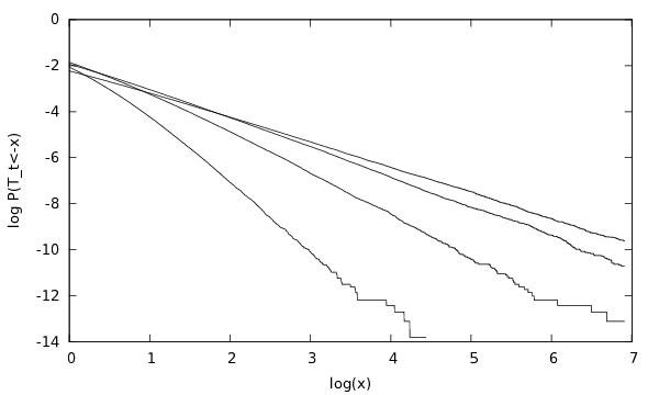
Refer to caption

Figure 3: Logarithmic plot of the empirical cumulative distribution function of 10610^{6} independent realizations of TtT_{t} (for t=40t=40), with parameter (from bottom to top) c=2c=2, c=3c=3, c=4c=4, c=5c=5.

6.2 A many particle system

In this section, we consider a more complex problem introduced in [34], and motivated by experimental studies of colloidal particles in optical traps. Let us consider Xtλ=(Yt1,⋯,YtN)X^{\lambda}_{t}=(Y^{1}_{t},\cdots,Y^{N}_{t}) where (Yti)i=1​…,N∈(ℝ2)N(Y^{i}_{t})_{i=1\,\ldots,N}\in(\mathbb{R}^{2})^{N} are the positions of NN two-dimensional particles evolving according to

d​Yti=−κ​Yti​d​t+∑j=1N∇U​(Yti−Ytj)​d​t+λ​e1​d​t+d​Wti, 1≤i≤N\mathrm{d}Y_{t}^{i}=-\kappa Y_{t}^{i}\mathrm{d}t+\sum_{j=1}^{N}\nabla U(Y_{t}^{i}-Y_{t}^{j})\mathrm{d}t+\lambda e_{1}\mathrm{d}t+\mathrm{d}W_{t}^{i},\;1\leq i\leq N (81)

with κ>0\kappa>0, λ∈ℝ\lambda\in\mathbb{R}, e1e_{1} the normed vector directed along the first coordinate, and U⁡(x)=Γ​e−|x|/|x|U(x)=\Gamma e^{-|x|}/|x|. The particles undergo a quadratic confining potential near the origin with strength κ\kappa, a repulsive interaction given by UU, a shear in the xx-direction with strength λ\lambda and a thermal noise.

We study the case of N=10N=10 particles with repulsion range Γ=25\Gamma=25 and attraction intensity κ=10\kappa=10 corresponding to the parameters studied in [34]. For those parameters, at equilibrium, particles are gathered around the origin. At λ=0\lambda=0, no particular direction appears in the dynamics, and the equilibrium measure is invariant with respect to rotations around the origin.

One wants to study the effect of shearing on the symmetry of the invariant measure. This symmetry can be measured by the empirical covariance Φ\Phi of the particle system, defined by

Φ⁡(Xtλ)=1N​∑i=1N(Yti,1−Y¯t1)​(Yti,2−Y¯t2),\Phi(X^{\lambda}_{t})=\frac{1}{N}\sum_{i=1}^{N}(Y_{t}^{i,1}-\bar{Y}_{t}^{1})(Y_{t}^{i,2}-\bar{Y}_{t}^{2}),

where Yti=(Yti,1,Yti,2)Y_{t}^{i}=(Y_{t}^{i,1},Y_{t}^{i,2}) and for k∈{1,2}k\in\{1,2\}, Y¯tk=1N​∑i=1NYti,k\bar{Y}_{t}^{k}=\frac{1}{N}\sum_{i=1}^{N}Y_{t}^{i,k}. One is interested in computing the derivative ∂λ0∫(ℝ2)NΦ​d​πλ\partial_{\lambda}^{0}\int_{(\mathbb{R}^{2})^{N}}\Phi\mathrm{d}\pi_{\lambda}.

On Figure 4, we plot the confidence interval obtained for the expectation 𝔼⁡[∂λ0Φ⁡(Xtλ)]\mathbb{E}[\partial_{\lambda}^{0}\Phi(X_{t}^{\lambda})], with N=105N=10^{5} independent simulations, as a function of the time tt. The dynamics (81) has been simulated using an explicit Euler-Maruyama scheme with time step δ​t=10−5\delta t=10^{-5}, and the expectation has been calculated through the Monte Carlo approximation

𝔼⁡[∂λ0Φ⁡(Xtλ)]=𝔼⁡[Tt⋅∇Φ​(Xt0)]≃1N​∑i=1NTti⋅∇Φ​(Xt0,i)\mathbb{E}[\partial_{\lambda}^{0}\Phi(X_{t}^{\lambda})]=\mathbb{E}[T_{t}\cdot\nabla\Phi(X_{t}^{0})]\simeq\frac{1}{N}\sum_{i=1}^{N}T_{t}^{i}\cdot\nabla\Phi(X_{t}^{0,i})

where the (Xt0,i,Tti)1≤i≤N(X_{t}^{0,i},T_{t}^{i})_{1\leq i\leq N} are independent simulations of the Euler-Maruyama discretization of the dynamics (7) ruling the evolution of (Xt0,Tt)(X_{t}^{0},T_{t}). As in [34], we observe that the correlation function 𝔼⁡[∂λ0Φ⁡(Xtλ)]\mathbb{E}[\partial_{\lambda}^{0}\Phi(X_{t}^{\lambda})] increases as a function of time, before reaching a plateau. We have checked that similar results are obtained using a finite differenciation instead of the simulation of the couple (Xt0,Tt)(X^{0}_{t},T_{t}).

Refer to caption

Figure 4: Sensitivity of the covariance with respect to the shear.

6.3 Particle merging

As mentioned in Section 6.1, in some situations, the variance of the tangent vector may become very large (or even infinite) which means that the estimators (10) and (11) become ineffective. Therefore, it is desirable to introduce variance reduction mechanisms. We explore in this section a first idea in the simple one-dimensional test case of Section 6.1. Extensions and further variance reduction techniques will be the subject of forthcoming works.

A first simple idea to reduce the variance is to replace the tangent vector TsT_{s} in the estimator of 𝔼⁡[∇f​(Xs0)⋅Ts]\mathbb{E}[\nabla f(X_{s}^{0})\cdot T_{s}] by its conditional expectation given Xs0X^{0}_{s}. This corresponds in practice to replacing the tangent vector of particles which are at the same position at a given time ss by the average of their tangent vectors. Then, the particles evolve again following the dynamics (7). We refer to this procedure as “particle merging”. In practice, with this naive procedure the probability to observe two particles at the same position is zero, in dimension larger than one. A first simple practical way to implement this technique is to introduce small subsets of the configuration space, and to merge particles which are in the same subset, which of course reduces the variance but introduce some bias. The merging can be performed in a much efficient way and in larger dimensions, by correlating the particles, see e.g. [20]. This will be the scope of future work. Before studying the interest of particle merging on the simple case of Section 6.1, let us first state the theoretical result which justifies the use of this approach.

Lemma 44.

Assume (min Spec). For s≥0s\geq 0, let (T~t)t≥s(\tilde{T}_{t})_{t\geq s} be the solution to

{d​T~td​t=∂λ0Fλ​(Xt0)−∇2(Xt0)​T~t​ , for all ​t≥s,T~s=𝔼⁡[Ts|Xs0].\left\{\begin{aligned} \frac{\mathrm{d}\tilde{T}_{t}}{\mathrm{d}t}&=\partial_{\lambda}^{0}F_{\lambda}(X_{t}^{0})-\nabla^{2}(X_{t}^{0})\tilde{T}_{t}\text{ , for all }\penalty\ t\geq s,\\ \tilde{T}_{s}&=\mathbb{E}[T_{s}|X_{s}^{0}].\end{aligned}\right.

Then ∀t≥s,T~t=𝔼[Tt|Xs0,(Wr−Ws)r∈[s,t]]\forall t\geq s,\;\tilde{T}_{t}=\mathbb{E}[T_{t}|X^{0}_{s},(W_{r}-W_{s})_{r\in[s,t]}]. Assume moreover that f:ℝd→ℝdf:\mathbb{R}^{d}\to\mathbb{R}^{d} is a Lipschitz function belonging to 𝕃p​(e−V⁡(x)​d​x)\mathbb{L}^{p}(e^{-V(x)}\mathrm{d}x) for some p∈[1,∞]p\in[1,\infty] and that the initial condition X0X_{0} to (1) admits a density with respect to π0\pi_{0} belonging to 𝕃pp−1​(e−V⁡(x)​d​x)\mathbb{L}^{\frac{p}{p-1}}(e^{-V(x)}\mathrm{d}x) (where, by convention, pp−1=∞\frac{p}{p-1}=\infty if p=1p=1). Then, for each t≥0t\geq 0, f⁡(Xtλ)f(X_{t}^{\lambda}) is integrable for λ∈[0,λ0]\lambda\in[0,\lambda_{0}], λ↦𝔼⁡[f⁡(Xtλ)]\lambda\mapsto\mathbb{E}[f(X_{t}^{\lambda})] is differentiable at λ=0\lambda=0 and

∂λ0(𝔼⁡[f⁡(Xtλ)])=𝔼⁡[∇f​(Xt0)⋅Tt]=𝔼⁡[∇f​(Xt0)⋅T~t], for each ​t≥s.\partial_{\lambda}^{0}\left(\mathbb{E}[f(X_{t}^{\lambda})]\right)=\mathbb{E}[\nabla f(X_{t}^{0})\cdot T_{t}]=\mathbb{E}[\nabla f(X_{t}^{0})\cdot\tilde{T}_{t}],\mbox{ for each }t\geq s.

This Lemma shows that if, at a given time ss, the particles at position Xs0X^{0}_{s} replace their current tangent vectors by an average of these tangent vectors, and then follow the dynamics (7) for t≥st\geq s, the estimator (11) is still consistent.

Proof.

By Lemma 23, Assumption (min Spec) ensures that TtT_{t} is integrable for each t≥0t\geq 0. In view of the equality (56) and using the semigroup property (55) of RX0R_{X^{0}}, one gets that for t≥s≥0t\geq s\geq 0,

Tt=RX0​(s,t)​Ts+∫stRX0​(r,t)​∂λ0Fλ​(Xr0)​𝑑r.T_{t}=R_{X^{0}}(s,t)T_{s}+\int_{s}^{t}R_{X^{0}}(r,t)\partial_{\lambda}^{0}F_{\lambda}(X_{r}^{0})dr.

Since (Xr0)r∈[s,t](X^{0}_{r})_{r\in[s,t]} and therefore (RX0​(r,t))r∈[s,t](R_{X^{0}}(r,t))_{r\in[s,t]} are measurable with respect to the sigma-field generated by Xs0X^{0}_{s} and (Wr−Ws)r∈[s,t](W_{r}-W_{s})_{r\in[s,t]}, one deduces that

𝔼[Tt|Xs0,(Wr−Ws)r∈[s,t]]=RX0(s,t)𝔼[Ts|Xs0,(Wr−Ws)r∈[s,t]]+∫stRX0(r,t)∂λ0Fλ(Xr0)dr.\mathbb{E}[T_{t}|X^{0}_{s},(W_{r}-W_{s})_{r\in[s,t]}]=R_{X^{0}}(s,t)\mathbb{E}[T_{s}|X^{0}_{s},(W_{r}-W_{s})_{r\in[s,t]}]+\int_{s}^{t}R_{X^{0}}(r,t)\partial_{\lambda}^{0}F_{\lambda}(X_{r}^{0})dr.

The independence of (Xs0,Ts)(X^{0}_{s},T_{s}) and (Wr−Ws)r∈[s,t](W_{r}-W_{s})_{r\in[s,t]} implies that 𝔼[Ts|Xs0,(Wr−Ws)r∈[s,t]]=𝔼[Ts|Xs0]\mathbb{E}[T_{s}|X^{0}_{s},(W_{r}-W_{s})_{r\in[s,t]}]=\mathbb{E}[T_{s}|X^{0}_{s}]. Since, by an adaptation of Proposition 20,

T~t=RX0​(s,t)​𝔼​[Ts|Xs0]+∫stRX0​(r,t)​∂λ0Fλ​(Xr0)​𝑑r,\tilde{T}_{t}=R_{X^{0}}(s,t)\mathbb{E}[T_{s}|X^{0}_{s}]+\int_{s}^{t}R_{X^{0}}(r,t)\partial_{\lambda}^{0}F_{\lambda}(X_{r}^{0})dr,

one concludes that T~t=𝔼[Tt|Xs0,(Wr−Ws)r∈[s,t]]\tilde{T}_{t}=\mathbb{E}[T_{t}|X^{0}_{s},(W_{r}-W_{s})_{r\in[s,t]}].

If the initial condition X0X_{0} to (1) admits a density with respect to π0\pi_{0} belonging to 𝕃pp−1​(e−V⁡(x)​d​x)\mathbb{L}^{\frac{p}{p-1}}(e^{-V(x)}\mathrm{d}x), then so does Xt0X^{0}_{t} for each t≥0t\geq 0 by Lemma 4. When f:ℝd→ℝdf:\mathbb{R}^{d}\to\mathbb{R}^{d} is a Lipschitz function belonging to 𝕃p​(e−V⁡(x)​d​x)\mathbb{L}^{p}(e^{-V(x)}\mathrm{d}x), the integrability of 𝔼⁡[f⁡(Xtλ)]\mathbb{E}[f(X_{t}^{\lambda})], the differentiability of λ↦𝔼⁡[f⁡(Xtλ)]\lambda\mapsto\mathbb{E}[f(X_{t}^{\lambda})] at λ=0\lambda=0 and the equality ∂λ0(𝔼⁡[f⁡(Xtλ)])=𝔼⁡[∇f​(Xt0)⋅Tt]\partial_{\lambda}^{0}\left(\mathbb{E}[f(X_{t}^{\lambda})]\right)=\mathbb{E}[\nabla f(X_{t}^{0})\cdot T_{t}] are deduced from an adaptation of the beginning of the proof of Theorem 33. Now, for t≥st\geq s,

𝔼⁡[∇f​(Xt0)⋅Tt]\displaystyle\mathbb{E}[\nabla f(X_{t}^{0})\cdot T_{t}] =𝔼[𝔼[∇f(Xt0)⋅Tt|Xs0,(Wr−Ws)r∈[s,t]]]\displaystyle=\mathbb{E}[\mathbb{E}[\nabla f(X_{t}^{0})\cdot T_{t}|X^{0}_{s},(W_{r}-W_{s})_{r\in[s,t]}]]
=𝔼[∇f(Xt0)⋅𝔼[Tt|Xs0,(Wr−Ws)r∈[s,t]]]=𝔼[∇f(Xt0)⋅T~t].\displaystyle=\mathbb{E}[\nabla f(X_{t}^{0})\cdot\mathbb{E}[T_{t}|X^{0}_{s},(W_{r}-W_{s})_{r\in[s,t]}]]=\mathbb{E}[\nabla f(X_{t}^{0})\cdot\tilde{T}_{t}].

∎

To test the interest of this approach, we consider again the setting of Section 6.1 with c=2.9c=2.9 (which corresponds to case where the variance of tangent vector TtT_{t}, at t=40t=40, is very large, see Figure 2). The merging procedure is done as follows: a uniform mesh with step size 0.040.04 is introduced, and, every ten timesteps, the tangent vectors of particles which are in the same bin are replaced by an average of these tangent vectors. On Figure 5, we observe that this procedure divides approximately the variance by 4, while introducing a bias which is sufficiently small so that the confidence interval of the simulation with merging is included in the confidence interval of the simulation without merging. Figure 6 then gives more quantitative estimates of the variances of these two simulations (with and without merging), as a function of time. We have observed numerically that large values of TtT_{t} become very unlikely with the merging procedure: using 10310^{3} independant realizations of 10310^{3} interacting particles over the time interval (0,10)(0,10), we did not observe any realization of TtT_{t} with absolute value larger than 33 (compare with what is reported on Figure 3).

Refer to caption

Figure 5: Empirical average and 95%-confidence interval for the Monte Carlo estimator of ∂λ𝔼⁡[f⁡(Xtλ)]\partial_{\lambda}\mathbb{E}[f(X_{t}^{\lambda})] as a function of time, ff being a smooth approximation of the the indicator function of ℝ+\mathbb{R}_{+}: f⁡(x)=12+1π​arctan⁡(10​x)f(x)=\frac{1}{2}+\frac{1}{\pi}\arctan(10x). The estimator is built with 10610^{6} realizations. Green: with merging (10310^{3} independent relizations of 10310^{3} interacting particles); Red: without merging (10610^{6} independent relizations).

Refer to caption

Figure 6: Empirical variance for the Monte Carlo estimator of ∂λ𝔼⁡[f⁡(Xtλ)]\partial_{\lambda}\mathbb{E}[f(X_{t}^{\lambda})] as a function of time, ff being the indicator function of ℝ+\mathbb{R}_{+}. Green: with merging ; Red: without merging.

Appendix A Alternative bounds on the density of Xt0X^{0}_{t}

In this section, we would like to present a few results which can be obtained under the assumption

Assumption (V).

The function VV is of class 𝒞2\mathcal{\mathcal{C}}^{2} and satisfies

CV=supx∈ℝd(2​Δ​V​(x)−|∇V​(x)|2)<+∞.C_{V}=\sup_{x\in{\mathbb{R}^{d}}}(2\Delta V(x)-|\nabla V(x)|^{2})<+\infty.

Note that simple assumptions on the quantity aV​(x)=2​Δ​V​(x)−|∇V​(x)|2a_{V}(x)=2\Delta V(x)-|\nabla V(x)|^{2} can give strong results on the equilibrium measure e−V⁡(x)​d​xe^{-V(x)}\mathrm{d}x. For instance, if aV​(x)a_{V}(x) goes to −∞-\infty at infinity, then the equilibrium measures satisfies a Poincaré inequality (see for example the appendix in [32]).

A.1 Bounds on the density of Xt0X^{0}_{t}

Proposition 45.

Consider the setting and the notation of Lemma 4 and let Assumption (V) hold. Assume that the measure e12​V​d​μ0e^{\frac{1}{2}V}\mathrm{d}\mu_{0} can be written as

e12​V​(x)​d​μ0=f⁡(x)​d​x+d​ν,e^{\frac{1}{2}V(x)}\mathrm{d}\mu_{0}=f(x)\mathrm{d}x+\mathrm{d}\nu,

where ff is some function in 𝕃p​(d​x)\mathbb{L}^{p}(\mathrm{d}x) with p∈[1,2]p\in[1,2] and ν\nu is some finite measure on ℝd{\mathbb{R}^{d}}. Then, for any t>0t>0, μt\mu_{t} is absolutely continuous with respect to e−12​V​(x)​d​xe^{-\frac{1}{2}V(x)}\mathrm{d}x with

‖d​μte−12​V​(x)​d​x‖𝕃2​(d​x)≤C​eC​t​(Cpt(1/p−1/2)​d/2+ν⁡(ℝd)td/4).\left\|\frac{\mathrm{d}\mu_{t}}{e^{-\frac{1}{2}V(x)}\mathrm{d}x}\right\|_{\mathbb{L}^{2}(\mathrm{d}x)}\leq Ce^{Ct}\left(\frac{C_{p}}{t^{(1/p-1/2)d/2}}+\frac{\nu({\mathbb{R}^{d}})}{t^{d/4}}\right). (82)
Proof.

Let ψ:ℝd→ℝ\psi:\mathbb{R}^{d}\to\mathbb{R} be a bounded measurable function and recall the formula

𝔼⁡[ψ⁡(Xt0)]=𝔼⁡[ψ⁡(X0+2​Wt)​e−12​V​(X0+2​Wt)​e12​V​(X0)​e14​∫0t(2​Δ​V−|∇V|2)​(X0+2​Ws)​𝑑s]\mathbb{E}[\psi(X_{t}^{0})]=\mathbb{E}\left[\psi(X_{0}+\sqrt{2}W_{t})e^{-\frac{1}{2}V(X_{0}+\sqrt{2}W_{t})}e^{\frac{1}{2}V(X_{0})}e^{\frac{1}{4}\int_{0}^{t}\left(2\Delta V-|\nabla V|^{2}\right)(X_{0}+\sqrt{2}W_{s})\mathrm{d}s}\right]

obtained by the Girsanov theorem, see Equation (15).

If CC is an upper bound for 14​(2​Δ​V−|∇V|2)\frac{1}{4}(2\Delta V-|\nabla V|^{2}), and if one assumes ψ≥0\psi\geq 0, one obtains

∫ℝdψ​d​μt\displaystyle\int_{\mathbb{R}^{d}}\psi\mathrm{d}\mu_{t} ≤eC​t​𝔼​[ψ⁡(X0+2​Wt)​e−12​V​(X0+2​Wt)​e12​V​(X0)]\displaystyle\leq e^{Ct}\mathbb{E}\left[\psi(X_{0}+\sqrt{2}W_{t})e^{-\frac{1}{2}V(X_{0}+\sqrt{2}W_{t})}e^{\frac{1}{2}V(X_{0})}\right]
=eC​t(4​π​t)d/2​∫ℝdψ⁡(y)​e−12​V​(y)​(∫ℝde12​V​(x)​e−|y−x|24​t​d​μ0​(x))​𝑑y.\displaystyle=\frac{e^{Ct}}{(4\pi t)^{d/2}}\int_{\mathbb{R}^{d}}\psi(y)e^{-\frac{1}{2}V(y)}\left(\int_{\mathbb{R}^{d}}e^{\frac{1}{2}V(x)}e^{-\frac{|y-x|^{2}}{4t}}\mathrm{d}\mu_{0}(x)\right)\mathrm{d}y.

so that μt≪e−12​V​(x)​d​x\mu_{t}\ll e^{-\frac{1}{2}V(x)}\mathrm{d}x with a Radon-Nikodym derivative d​μte−12​V​(x)​d​x\frac{\mathrm{d}\mu_{t}}{e^{-\frac{1}{2}V(x)}\mathrm{d}x} satisfying

d​μte−12​V​(x)​d​x\displaystyle\frac{\mathrm{d}\mu_{t}}{e^{-\frac{1}{2}V(x)}\mathrm{d}x} ≤eC​t​(e12​V​μ0)∗γt=eC​t​(f∗γt+ν∗γt),\displaystyle\leq e^{Ct}\left(e^{\frac{1}{2}V}\mu_{0}\right)*\gamma_{t}=e^{Ct}\left(f*\gamma_{t}+\nu*\gamma_{t}\right),

where ∗* stands for the convolution product, and γt​(x)=1(4​π​t)d/2​e−|x|24​t\gamma_{t}(x)=\frac{1}{(4\pi t)^{d/2}}e^{-\frac{|x|^{2}}{4t}} denotes the centered Gaussian density with covariance matrix 2​t​Id2tI_{d}. One concludes that (82) holds by:

  • •

    the Young inequality ‖f∗γt‖𝕃2​(d​x)≤‖f‖𝕃p​(d​x)​‖γt‖𝕃q​(d​x)\|f*\gamma_{t}\|_{\mathbb{L}^{2}(\mathrm{d}x)}\leq\|f\|_{\mathbb{L}^{p}(\mathrm{d}x)}\|\gamma_{t}\|_{\mathbb{L}^{q}(\mathrm{d}x)} where 1/p+1/q=3/21/p+1/q=3/2 (p,q∈[1,∞]p,q\in[1,\infty]) and the heat kernel estimate ‖γt‖𝕃q​(d​x)≤Cq​t−(1−1q)​d2\|\gamma_{t}\|_{\mathbb{L}^{q}(\mathrm{d}x)}\leq C_{q}t^{-\left(1-\frac{1}{q}\right)\frac{d}{2}};

  • •

    the estimate ‖ν∗γt‖𝕃2​(d​x)2≤‖ν∗γt‖𝕃1​(d​x)​‖ν∗γt‖𝕃∞​(d​x)≤(ν⁡(ℝd))2(4​π​t)d/2\|\nu*\gamma_{t}\|^{2}_{\mathbb{L}^{2}(\mathrm{d}x)}\leq\|\nu*\gamma_{t}\|_{\mathbb{L}^{1}(\mathrm{d}x)}\|\nu*\gamma_{t}\|_{\mathbb{L}^{\infty}(\mathrm{d}x)}\leq\frac{(\nu({\mathbb{R}^{d}}))^{2}}{(4\pi t)^{d/2}}.

∎

A.2 An additional result

Assumption (V) can also be useful to prove the second point in Assumption (Pot)-(i​i)(ii) on the potential VV.

Lemma 46.

Under Assumption (V), the function ∇V\nabla V is in 𝕃2​(e−V⁡(x)​d​x)\mathbb{L}^{2}(e^{-V(x)}\mathrm{d}x):

∫ℝd|∇V|2​(x)​e−V⁡(x)​𝑑x≤CV.\int_{\mathbb{R}^{d}}|\nabla V|^{2}(x)e^{-V(x)}\mathrm{d}x\leq C_{V}.
Proof.

Let χn​(x)=χ⁡(x/n)\chi_{n}(x)=\chi(x/n) where χ\chi is a smooth, [0,1][0,1]-valued, cutoff function such that χ⁡(x)=1\chi(x)=1 for |x|<1|x|<1 and χ⁡(x)=0\chi(x)=0 for |x|>2|x|>2.

∫ℝd|∇V|2​(x)​χn​(x)​e−V⁡(x)​𝑑x\displaystyle\int_{\mathbb{R}^{d}}|\nabla V|^{2}(x)\chi_{n}(x)e^{-V(x)}\mathrm{d}x =−∫ℝd(χn(x)∇V(x))⋅∇e−V⁡(x)dx\displaystyle=-\int_{\mathbb{R}^{d}}\left(\chi_{n}(x)\nabla V(x)\right)\cdot\nabla e^{-V(x)}\mathrm{d}x
=∫ℝd∇χn​(x)⋅∇V​(x)​e−V⁡(x)​𝑑x+∫ℝdχn​(x)​Δ​V​(x)​e−V⁡(x)​𝑑x\displaystyle=\int_{\mathbb{R}^{d}}\nabla\chi_{n}(x)\cdot\nabla V(x)e^{-V(x)}\mathrm{d}x+\int_{\mathbb{R}^{d}}\chi_{n}(x)\Delta V(x)e^{-V(x)}\mathrm{d}x
≤∫ℝdΔ​χn​(x)​e−V⁡(x)​𝑑x+12​∫ℝdχn​(x)​|∇V|2​(x)​e−V⁡(x)​𝑑x+12​CV.\displaystyle\leq\int_{\mathbb{R}^{d}}\Delta\chi_{n}(x)e^{-V(x)}\mathrm{d}x+\frac{1}{2}\int_{\mathbb{R}^{d}}\chi_{n}(x)|\nabla V|^{2}(x)e^{-V(x)}\mathrm{d}x+\frac{1}{2}C_{V}.

As a consequence,

∫ℝd|∇V|2​(x)​χn​(x)​e−V⁡(x)​𝑑x≤2​∫ℝdΔ​χn​(x)​e−V⁡(x)​𝑑x+CV\int_{\mathbb{R}^{d}}|\nabla V|^{2}(x)\chi_{n}(x)e^{-V(x)}\mathrm{d}x\leq 2\int_{\mathbb{R}^{d}}\Delta\chi_{n}(x)e^{-V(x)}\mathrm{d}x+C_{V}

and the result follows from taking n→∞n\to\infty by Fatou’s lemma for the left-hand side and Lebesgue’s theorem for the right-hand side. ∎

Appendix B About the Assumption (Conv)

In this section, we show that Assumption (Conv) is a natural one, since it appears as a sufficient condition in another related problem.

We recall that (Ytx)t≥0(Y^{x}_{t})_{t\geq 0} is defined in (12) as the solution to

∀t≥0,Ytx=x−∫0t∇V​(Ysx)​𝑑s+2​Wt.\forall t\geq 0,\penalty\ Y^{x}_{t}=x-\int_{0}^{t}\nabla V(Y^{x}_{s})\mathrm{d}s+\sqrt{2}W_{t}. (83)

Since (RYx​(0,t))t≥0(R_{Y^{x}}(0,t))_{t\geq 0} is the differential of the trajectory (Ytx)t≥0(Y^{x}_{t})_{t\geq 0} with respect to xx, we expect that a condition yielding long-time decay for RYxR_{Y^{x}} will imply that trajectories with same noise and close initial conditions will eventually converge toward each other. More precisely, we are interested in the joint long-time behavior of the so-called duplicated dynamics (Ytx,Yty)t≥0(Y_{t}^{x},Y_{t}^{y})_{t\geq 0}, where xx and yy are two different initial conditions. Note here that the two processes (Ytx)t≥0(Y^{x}_{t})_{t\geq 0} and (Yty)t≥0(Y^{y}_{t})_{t\geq 0} are driven by the same Brownian motion.

In [23], the same problem is considered for a diffusion whose diffusion matrix may not be constant. In that case, an example is provided, where the process Ytx−YtyY_{t}^{x}-Y_{t}^{y} does not converge to 00.

A similar problem is considered in [5]: the process is a Brownian motion reflected on the boundary of a domain Ω\Omega. Such a dynamics can be formally seen as a singular case of the problem we consider, with V=∞×𝟏ΩcV=\infty\times\mathbf{1}_{\Omega^{c}}. Equation (83) then has to be written with a local time on the boundary in place of ∇V\nabla V. In that case, the difference Ytx−YtyY_{t}^{x}-Y_{t}^{y} will converge to 00 if the domain Ω\Omega is smooth enough and has at most one hole. However, it is conjectured that the same result holds for much more general domains.

We will use the fact that VV is such that the dynamics (83) is ergodic with respect to the invariant measure e−V⁡(x)​d​xe^{-V(x)}\mathrm{d}x.

B.1 The one-dimensional case

In the one-dimensional case, this question is especially simple, because of the order structure on the state space. In particular (see [23]), it can be checked that if for any x∈ℝx\in\mathbb{R}, YtxY_{t}^{x} converge weakly to π0\pi_{0} as t→∞t\to\infty, then the only invariant distribution of the duplicated dynamics is the image of e−V⁡(x)​d​xe^{-V(x)}\mathrm{d}x by x↦(x,x)x\mapsto(x,x). Actually, under additional assumption, one can show that Ytx−YtyY^{x}_{t}-Y^{y}_{t} converges in mean to 00 in the long-time limit.

Proposition 47.

Assume that the dimension is d=1d=1. If for any x∈ℝx\in\mathbb{R} the time marginals of the process (Ytx)t≥0(Y_{t}^{x})_{t\geq 0} converge weakly to π0\pi_{0} as t→∞t\to\infty and the random variables (Ytx)t≥0(Y_{t}^{x})_{t\geq 0} are uniformly integrable, then, for any x,y∈ℝx,y\in\mathbb{R}, the process (Ytx−Yty)t≥0(Y_{t}^{x}-Y_{t}^{y})_{t\geq 0} converges to 00 in 𝕃1​(Ω)\mathbb{L}^{1}(\Omega).

According to Corollary 12, the long-time convergence of the marginals holds for instance if the potential VV satisfies a Poincaré inequality (see Assumption (Poinc(η\eta))).

Proof.

First, from the uniform integrability of (Xtx)t≥0(X_{t}^{x})_{t\geq 0} and the weak convergence of the time marginals, both 𝔼⁡[Ytx]\mathbb{E}[Y_{t}^{x}] and 𝔼⁡[Yty]\mathbb{E}[Y_{t}^{y}] converge to ∫ℝx​e−V⁡(x)​𝑑x\int_{\mathbb{R}}xe^{-V(x)}\mathrm{d}x as t→∞t\to\infty.

Now assume, without loss of generality that x≤yx\leq y. Then, from a comparison theorem, Ytx≤YtyY_{t}^{x}\leq Y_{t}^{y} holds for all positive times, and one obtains

𝔼⁡[|Ytx−Yty|]=𝔼⁡[Ytx−Yty]=𝔼⁡[Ytx]−𝔼⁡[Yty]→0.\mathbb{E}[|Y_{t}^{x}-Y_{t}^{y}|]=\mathbb{E}[Y_{t}^{x}-Y_{t}^{y}]=\mathbb{E}[Y_{t}^{x}]-\mathbb{E}[Y_{t}^{y}]\to 0.

∎

B.2 A general criterion

Proposition 48.

The following facts hold true:

  1. 1.

    Assume that

    ∀x,y∈ℝd,(x−y)⋅(∇V​(x)−∇V​(y))≥v⁡(x)+v⁡(y)2​|x−y|2\forall x,y\in{\mathbb{R}^{d}},\;(x-y)\cdot(\nabla V(x)-\nabla V(y))\geq\frac{v(x)+v(y)}{2}|x-y|^{2} (84)

    with v:ℝd→ℝv:{\mathbb{R}^{d}}\to\mathbb{R} such that ∫ℝdmax⁡(0,−v⁡(x))​e−V⁡(x)​𝑑x<∞\int_{\mathbb{R}^{d}}\max(0,-v(x))e^{-V(x)}\mathrm{d}x<\infty and ∫ℝdv⁡(x)​e−V⁡(x)​𝑑x>0\int_{\mathbb{R}^{d}}v(x)e^{-V(x)}\mathrm{d}x>0. Then for all x,y∈ℝdx,y\in{\mathbb{R}^{d}}, |Ytx−Yty||Y^{x}_{t}-Y^{y}_{t}| converges a.s. to 00, exponentially fast at any rate between 00 and ∫ℝdv⁡(x)​e−V⁡(x)​𝑑x\int_{\mathbb{R}^{d}}v(x)e^{-V(x)}\mathrm{d}x as t→∞t\to\infty.

  2. 2.

    The exponential convergence to 00 still holds if VV is convex and there exist x0∈ℝdx_{0}\in{\mathbb{R}^{d}} and ε>0\varepsilon>0 such that the inequality infx∈B⁡(x0,ε)min⁡Spec⁡(∇2V​(x))>0\inf_{x\in B(x_{0},\varepsilon)}\min{\rm Spec}(\nabla^{2}V(x))>0 holds.

  3. 3.

    If VV is convex, then the only invariant measure of the duplicated dynamics is the image of e−V⁡(x)​d​xe^{-V(x)}\mathrm{d}x by x↦(x,x)x\mapsto(x,x).

Let us start with a few remarks:

Remark 49.
  • •

    The first point can be applied to the so-called Mexican hat potential V⁡(x)=β⁡(|x|4−γ​|x|2)V(x)=\beta(|x|^{4}-\gamma|x|^{2}), with β>0\beta>0 and γ>0\gamma>0, in dimension d≥2d\geq 2. For this potential, one has

    (x−y)⋅(∇V​(x)−∇V​(y))\displaystyle(x-y)\cdot(\nabla V(x)-\nabla V(y)) =2​β​|x−y|2​(|x|2+|y|2−γ)+2​β​(|x|2−|y2|)2\displaystyle=2\beta|x-y|^{2}(|x|^{2}+|y|^{2}-\gamma)+2\beta(|x|^{2}-|y^{2}|)^{2}
    ≥v⁡(x)+v⁡(y)2​|x−y|2,\displaystyle\geq\frac{v(x)+v(y)}{2}|x-y|^{2},

    for v⁡(x)=β⁡(4​|x|2−2​γ)v(x)=\beta(4|x|^{2}-2\gamma). In addition, one has ∫ℝdv⁡(x)​e−V⁡(x)​𝑑x>0\int_{\mathbb{R}^{d}}v(x)e^{-V(x)}\mathrm{d}x>0 since

    ∫ℝd|x|2​eβ⁡(γ​|x|2−|x|4)​𝑑x∫ℝdeβ⁡(γ​|x|2−|x|4)​𝑑x\displaystyle\frac{\int_{\mathbb{R}^{d}}|x|^{2}e^{\beta(\gamma|x|^{2}-|x|^{4})}\mathrm{d}x}{\int_{\mathbb{R}^{d}}e^{\beta(\gamma|x|^{2}-|x|^{4})}\mathrm{d}x} =∫0+∞rd2​eβ⁡(γ​r−r2)​𝑑r∫0+∞rd2−1​eβ⁡(γ​r−r2)​𝑑r\displaystyle=\frac{\int_{0}^{+\infty}r^{\frac{d}{2}}e^{\beta(\gamma r-r^{2})}dr}{\int_{0}^{+\infty}r^{\frac{d}{2}-1}e^{\beta(\gamma r-r^{2})}dr}
    =γ2+∫0+∞rd2−1​(r−γ2)​eβ⁡(γ​r−r2)​𝑑r∫0+∞rd2−1​eβ⁡(γ​r−r2)​𝑑r\displaystyle=\frac{\gamma}{2}+\frac{\int_{0}^{+\infty}r^{\frac{d}{2}-1}(r-\frac{\gamma}{2})e^{\beta(\gamma r-r^{2})}dr}{\int_{0}^{+\infty}r^{\frac{d}{2}-1}e^{\beta(\gamma r-r^{2})}dr}
    =γ2+1{d=2}2​β​∫0+∞eβ⁡(γ​r−r2)​𝑑r+1{d>2}(d−2)​∫0+∞rd2−2​eβ⁡(γ​r−r2)​𝑑r4​β​∫0+∞rd2−1​eβ⁡(γ​r−r2)​𝑑r\displaystyle=\frac{\gamma}{2}+\frac{1_{\{d=2\}}}{2\beta\int_{0}^{+\infty}e^{\beta(\gamma r-r^{2})}dr}+1_{\{d>2\}}\frac{(d-2)\int_{0}^{+\infty}r^{\frac{d}{2}-2}e^{\beta(\gamma r-r^{2})}dr}{4\beta\int_{0}^{+\infty}r^{\frac{d}{2}-1}e^{\beta(\gamma r-r^{2})}dr}
    >γ2.\displaystyle>\frac{\gamma}{2}.
  • •

    Letting y→xy\to x in (84), one obtains that ∀x∈ℝd\forall x\in{\mathbb{R}^{d}}, v⁡(x)≤min⁡Spec⁡(∇2V​(x))v(x)\leq\min{\rm Spec}(\nabla^{2}V(x)). When x↦min⁡Spec⁡(∇2V​(x))x\mapsto\min{\rm Spec}(\nabla^{2}V(x)) is concave,

    (x−y)⋅(∇V​(x)−∇V​(y))\displaystyle(x-y)\cdot(\nabla V(x)-\nabla V(y)) =∫01(x−y)⋅∇2V​(θ​x+(1−θ)​y)​(x−y)​𝑑θ\displaystyle=\int_{0}^{1}(x-y)\cdot\nabla^{2}V(\theta x+(1-\theta)y)(x-y)\mathrm{d}\theta
    ≥|x−y|∫012⁡min⁡Spec⁡(∇2V​(θ​x+(1−θ)​y))​𝑑θ\displaystyle\geq|x-y|^{2}\int_{0}^{1}\min{\rm Spec}(\nabla^{2}V(\theta x+(1-\theta)y))\mathrm{d}\theta
    ≥|x−y|2​∫01θ​min⁡Spec⁡(∇2V​(x))+(1−θ)​min⁡Spec⁡(∇2V​(y))​𝑑θ\displaystyle\geq|x-y|^{2}\int_{0}^{1}\theta\min{\rm Spec}(\nabla^{2}V(x))+(1-\theta)\min{\rm Spec}(\nabla^{2}V(y))\mathrm{d}\theta
    ≥12​(min⁡Spec⁡(∇2V​(x))+min⁡Spec⁡(∇2V​(y)))​|x−y|2\displaystyle\geq\frac{1}{2}\left(\min{\rm Spec}(\nabla^{2}V(x))+\min{\rm Spec}(\nabla^{2}V(y))\right)|x-y|^{2}

    and one may choose v⁡(x)=min⁡Spec⁡(∇2V​(x))v(x)=\min{\rm Spec}(\nabla^{2}V(x)) in (84).

  • •

    When V=V¯+V^V=\bar{V}+\hat{V} with V¯\bar{V} such that x↦min⁡Spec⁡(∇2V¯​(x))x\mapsto\min{\rm Spec}(\nabla^{2}\bar{V}(x)) is concave and V^\hat{V} such that x↦∇V^​(x)x\mapsto\nabla\hat{V}(x) is Lipschitz with constant δ\delta and constant outside some Borel subset AA of ℝd{\mathbb{R}^{d}}, then one may choose v⁡(x)=min⁡Spec⁡(∇2V¯​(x))−2​δ​1A​(x)v(x)=\min{\rm Spec}(\nabla^{2}\bar{V}(x))-2\delta 1_{A}(x) in (84).

Proof.
  1. 1.

    One has

    d​|Ytx−Yty|2\displaystyle\mathrm{d}|Y^{x}_{t}-Y^{y}_{t}|^{2} =−2(Ytx−Yty)⋅(∇V(Ytx)−∇V(Yty))dt\displaystyle=-2(Y^{x}_{t}-Y^{y}_{t})\cdot(\nabla V(Y^{x}_{t})-\nabla V(Y^{y}_{t}))\mathrm{d}t (85)
    ≤−(v⁡(Ytx)+v⁡(Yty))​|Ytx−Yty|2​d​t,\displaystyle\leq-(v(Y^{x}_{t})+v(Y^{y}_{t}))|Y^{x}_{t}-Y^{y}_{t}|^{2}\mathrm{d}t,

    under (84). Hence

    |Yxt−Yyt|2≤|x−y|2e−∫0t(v(Yxs)+v(Yys))ds.|Y^{x}_{t}-Y^{y}_{t}|^{2}\leq|x-y|^{2}e^{-\int_{0}^{t}(v(Y^{x}_{s})+v(Y^{y}_{s}))\mathrm{d}s}.

    Since, by (51), 1t​∫0t(v⁡(Ysx)+v⁡(Ysy))​𝑑s\frac{1}{t}\int_{0}^{t}(v(Y^{x}_{s})+v(Y^{y}_{s}))\mathrm{d}s converges a.s. to 2​∫ℝdv⁡(x)​e−V⁡(x)​𝑑x>02\int_{\mathbb{R}^{d}}v(x)e^{-V(x)}\mathrm{d}x>0, one easily deduces the first assertion.

  2. 2.

    When VV is convex, then t↦|Ytx−Yty|t\mapsto|Y^{x}_{t}-Y^{y}_{t}| is nonincreasing by (85). Now, for z∈B⁡(x0,ε2)z\in B(x_{0},\frac{\varepsilon}{2}) and w∈ℝdw\in{\mathbb{R}^{d}}, one has

    (z−w)⋅(∇V​(z)−∇V​(w))≥|z−w|​infB⁡(x0,ε)min⁡Spec⁡(∇2V​(⋅))​(ε2​1B​(x0,ε)c​(w)+|z−w|​1B⁡(x0,ε)​(w)).(z-w)\cdot(\nabla V(z)-\nabla V(w))\geq|z-w|\inf_{B(x_{0},\varepsilon)}\min{\rm Spec}(\nabla^{2}V(\cdot))\left(\frac{\varepsilon}{2}1_{B(x_{0},\varepsilon)^{c}}(w)+|z-w|1_{B(x_{0},\varepsilon)}(w)\right).

    As a consequence,

    (Ytx−Yty)⋅(∇V​(Ytx)−∇V​(Yty))≥1B⁡(x0,ε2)​(Ytx)​infB⁡(x0,ε)min⁡Spec⁡(∇2V​(⋅))​(ε2​|x−y|∧1)​|Ytx−Yty|2.(Y^{x}_{t}-Y^{y}_{t})\cdot(\nabla V(Y^{x}_{t})-\nabla V(Y^{y}_{t}))\geq 1_{B(x_{0},\frac{\varepsilon}{2})}(Y^{x}_{t})\inf_{B(x_{0},\varepsilon)}\hskip-3.0pt\min{\rm Spec}(\nabla^{2}V(\cdot))\left(\frac{\varepsilon}{2|x-y|}\wedge 1\right)|Y^{x}_{t}-Y^{y}_{t}|^{2}.

    One concludes by arguments similar to the ones used for the first assertion.

  3. 3.

    Let VV be convex and differentiable and let x≠yx\neq y be such that (x−y)⋅(∇V​(x)−∇V​(y))=0(x-y)\cdot(\nabla V(x)-\nabla V(y))=0. Then VV is affine on the segment [x,y][x,y] and V⁡(x+y2)=V⁡(x)+V⁡(y)2V(\frac{x+y}{2})=\frac{V(x)+V(y)}{2}. For z∈ℝd∖{0}z\in{\mathbb{R}^{d}}\setminus\{0\} and ε∈ℝ\varepsilon\in\mathbb{R},

    V⁡(x)+V⁡(y)2=V⁡(x+y2)\displaystyle\frac{V(x)+V(y)}{2}=V\left(\frac{x+y}{2}\right) ≤V⁡(x+ε​z)+V⁡(y−ε​z)2\displaystyle\leq\frac{V(x+\varepsilon z)+V(y-\varepsilon z)}{2}
    =V⁡(x)+V⁡(y)2+ε​z2⋅(∇V​(x)−∇V​(y))+o⁡(ε)\displaystyle=\frac{V(x)+V(y)}{2}+\frac{\varepsilon z}{2}\cdot(\nabla V(x)-\nabla V(y))+o(\varepsilon)

    as |ε|→0|\varepsilon|\to 0. As a consequence z⋅(∇V​(x)−∇V​(y))=0z\cdot(\nabla V(x)-\nabla V(y))=0 and ∇V​(x)=∇V​(y)\nabla V(x)=\nabla V(y).

    Let (Xt)t≥0(X_{t})_{t\geq 0} and (Yt)t≥0(Y_{t})_{t\geq 0} be two solutions to the stochastic differential equation (2), such that (X0,Y0)(X_{0},Y_{0}) is distributed according to some invariant probability measure of the duplicated dynamics. Since |Xt−Yt|2|X_{t}-Y_{t}|^{2} is a.s. non-increasing with tt and constant in distribution, a.s. t↦|Xt−Yt|2t\mapsto|X_{t}-Y_{t}|^{2} is constant and therefore d​t\mathrm{d}t-a.e. (Xt−Yt)⋅(∇V​(Xt)−∇V​(Yt))=0(X_{t}-Y_{t})\cdot(\nabla V(X_{t})-\nabla V(Y_{t}))=0 which implies ∇V​(Xt)=∇V​(Yt)\nabla V(X_{t})=\nabla V(Y_{t}). One deduces that a.s., t↦Xt−Ytt\mapsto X_{t}-Y_{t} is constant.
    Now, since x↦e−V⁡(x)x\mapsto e^{-V(x)} is integrable, then VV cannot be affine in some direction and for any z∈ℝd∖{0}z\in{\mathbb{R}^{d}}\setminus\{0\}, x↦z⋅(∇V​(x)−∇V​(x−z))x\mapsto z\cdot(\nabla V(x)-\nabla V(x-z)) is not constant equal to zero. By continuity of ∇V\nabla V, one deduces the existence of y∈ℝdy\in{\mathbb{R}^{d}} and ε>0\varepsilon>0 such that ∀x∈B⁡(y,ε)\forall x\in B(y,\varepsilon), z⋅(∇V​(x)−∇V​(x−z))>0z\cdot(\nabla V(x)-\nabla V(x-z))>0. With the ergodicity of (Xt)t≥0(X_{t})_{t\geq 0} and the fact that d​t\mathrm{d}t-a.e. (X0−Y0)⋅(∇V​(Xt)−∇V​(Xt−X0+Y0))=0(X_{0}-Y_{0})\cdot(\nabla V(X_{t})-\nabla V(X_{t}-X_{0}+Y_{0}))=0, one concludes that a.s. X0=Y0X_{0}=Y_{0}.

∎

Acknowledgements

This work is supported by the European Research Council under the European Union’s Seventh Framework Programme (FP/2007-2013) / ERC Grant Agreement number 614492 and by the French National Research Agency under the grant ANR-12-BS01-0019 (STAB). The authors would like to thank fruitful discussions with G. Stoltz on nonequilibrium methods and Green-Kubo formulae.

References

  • [1] C. Ané, S. Blachère, D. Chafaï, P. Fougères, I. Gentil, F. Malrieu, C. Roberto, and G. Scheffer. Sur les inégalités de Sobolev logarithmiques. Société Mathématique de France, 2000. In French.
  • [2] R. Assaraf, M. Caffarel, and A.C. Kollias. Chaotic versus nonchaotic stochastic dynamics in monte carlo simulations: A route for accurate energy differences in nn-body systems. Phys. Rev. Lett., 106:150601, 2011.
  • [3] V. Bally, M.P. Bavouzet, and M. Messaoud. Integration by parts formula for locally smooth laws and applications to sensitivity computations. Ann. Appl. Prob., 17:33–66, 2007.
  • [4] S. Bobkov and M. Ledoux. Poincaré’s inequalities and Talagrand’s concentration phenomenon for the exponential distribution. Probab. Theory Related Fields, 107(3):383–400, 1997.
  • [5] K. Burdzy, Z.-Q. Chen, and P. Jones. Synchronous couplings of reflected brownian motions in smooth domains. Illinois Journal of Mathematics, 50(1-4):189–268, 2006.
  • [6] D. Chandler. Introduction to Modern Statistical Mechanics. Oxford University Press, 1987.
  • [7] J. Chen, G. Zhang, and B. Li. How to improve the accuracy of equilibrium molecular dynamics for computation of thermal conductivity? Physics Letters A, 374(23):2392 – 2396, 2010.
  • [8] G. Ciccotti and G. Jacucci. Direct computation of dynamical response by molecular-dynamics - mobility of a charged Lennard-Jones particle. Physical Review Letters, 35(12):789–792, 1975.
  • [9] G. Ciccotti, R. Kapral, and A. Sergi. Non-equilibrium molecular dynamics. In S. Yip, editor, Handbook of Materials Modeling, pages 745–761. Springer Netherlands, 2005.
  • [10] M. Cwikel. Weak type estimates for singular values and the number of bound states of Schrödinger operators. Ann. of Math. (2), 106(1):93–100, 1977.
  • [11] F. den Hollander. Large deviations, volume 14 of Fields Institute Monographs. American Mathematical Society, Providence, RI, 2000.
  • [12] M. Duflo. Random iterative models. Springer, 1997.
  • [13] K.D. Elworthy and X.M. Li. Formulae for the derivatives of heat semigroups. J. Func. Anal., 125:252–286, 1994.
  • [14] D.J. Evans and G. Morriss. Statistical mechanics of nonequilibrium liquids. Cambridge University Press, 2008.
  • [15] J. Fontbona and B. Jourdain. On the long time behaviour of stochastic vortices systems. Markov Process. Related Fields, 20(4):675–704, 2014.
  • [16] Ĭ.Ī. Gīhman and A.V. Skorohod. Stochastic differential equations. Springer-Verlag, New York-Heidelberg, 1972. Translated from the Russian by Kenneth Wickwire, Ergebnisse der Mathematik und ihrer Grenzgebiete, Band 72.
  • [17] D. Gilbarg and N.S. Trudinger. Elliptic partial differential equations of second order. Classics in Mathematics. Springer-Verlag, Berlin, 2001.
  • [18] M. Hairer and A.J. Majda. A simple framework to justify linear response theory. Nonlinearity, 23(4):909–922, 2010.
  • [19] Bismut J.M. Large deviations and the Malliavin calculus. Birkhäuser, 1984.
  • [20] M. H. Kalos and F. Pederiva. Exact monte carlo method for continuum fermion systems. Physical review letters, 85(17):3547, 2000.
  • [21] I. Karatzas and S.E. Shreve. Brownian motion and stochastic calculus. Springer-Verlag, 1988.
  • [22] N. V. Krylov. Lectures on elliptic and parabolic equations in Hölder spaces, volume 12 of Graduate Studies in Mathematics. American Mathematical Society, Providence, RI, 1996.
  • [23] V. Lemaire, G. Pagès, and F. Panloup. Invariant measure of duplicated diffusions and application to Richardson-Romberg extrapolation, 2013. http://arxiv.org/abs/1302.1651.
  • [24] E. Lieb. Bounds on the eigenvalues of the Laplace and Schroedinger operators. Bull. Amer. Math. Soc., 82(5):751–753, 1976.
  • [25] P. Malliavin. Integration and probability, volume 157 of Graduate Texts in Mathematics. Springer-Verlag, New York, 1995.
  • [26] A. Quarteroni and A. Valli. Numerical Approximation of Partial Differential Equations. Springer, 1997.
  • [27] L. Rey-Bellet. Ergodic properties of Markov processes. In Open quantum systems. II, volume 1881 of Lecture Notes in Math., pages 1–39. Springer, Berlin, 2006.
  • [28] G. V. Rozenbljum. Distribution of the discrete spectrum of singular differential operators. Dokl. Akad. Nauk SSSR, 202:1012–1015, 1972.
  • [29] T.H. Rydberg. A note on the existence of unique equivalent martingale measures in a markovian setting. Finance and Stochastics, 1(3):251–257, 1997.
  • [30] J. Tailleur and J. Kurchan. Probing rare physical trajectories with Lyapunov weighted dynamics. Nature Physics, 3:203–207, 2007.
  • [31] R. Temam. Navier-Stokes equations, volume 2 of Studies in Mathematics and its Applications. North-Holland Publishing Co., Amsterdam-New York, 1979.
  • [32] C. Villani. Hypocoercivity. Memoirs Amer. Math. Soc., 202, 2009.
  • [33] W. von Wahl. The equation u′+A⁡(t)​u=fu^{\prime}+A(t)u=f in a Hilbert space and LpL^{p}-estimates for parabolic equations. J. London Math. Soc. (2), 25(3):483–497, 1982.
  • [34] P.B. Warren and R.J. Allen. Malliavin weight sampling for computing sensitivity coefficients in brownian dynamics simulations. Physical Review Letters, 109(25):250601, 2012.