On Transitive Consistency for Linear Invertible Transformations between Euclidean Coordinate Systemsfootnoteinfo
Abstract
Transitive consistency is an intrinsic property for collections of linear invertible transformations between Euclidean coordinate frames. In practice, when the transformations are estimated from data, this property is lacking. This work addresses the problem of synchronizing transformations that are not transitively consistent. Once the transformations have been synchronized, they satisfy the transitive consistency condition – a transformation from frame to frame is equal to the composite transformation of first transforming to and then transforming to . The coordinate frames correspond to nodes in a graph and the transformations correspond to edges in the same graph. Two direct or centralized synchronization methods are presented for different graph topologies; the first one for quasi-strongly connected graphs, and the second one for connected graphs. As an extension of the second method, an iterative Gauss-Newton method is presented, which is later adapted to the case of affine and Euclidean transformations. Two distributed synchronization methods are also presented for orthogonal matrices, which can be seen as distributed versions of the two direct or centralized methods; they are similar in nature to standard consensus protocols used for distributed averaging. When the transformations are orthogonal matrices, a bound on the optimality gap can be computed. Simulations show that the gap is almost tight, even for noise large in magnitude. This work also contributes on a theoretical level by providing linear algebraic relationships for transitively consistent transformations. One of the benefits of the proposed methods is their simplicity – basic linear algebraic methods are used, e.g., the Singular Value Decomposition (SVD). For a wide range of parameter settings, the methods are numerically validated.
keywords
Distributed optimization, transformation synchronization, Procrustes problem, consensus algorithms, graph theory.footnoteinfo]The authors gratefully acknowledge the financial support from the Fonds National de la Recherche, Luxembourg (6538106, 8864515).
, ,
1 Introduction
Collections of linear invertible transformations between Euclidean coordinate systems must be transitively consistent. In practice however, when the transformations are estimated from data, this condition does not hold. This issue is present in the 3D localization problem, where transformations are rigid and estimated from e.g., camera measurements; in the multiple images registration problem where the transformations are affine (or linear by using homogeneous coordinates); in the generalized Procrustes problem where scales, rotations and translations are calculated from multiple point clouds. In order to resolve the issue, the estimated transformations need to be synchronized in the sense of finding transitively consistent transformations close to the estimated ones.
1.1 Problem
This work addresses the problem of synchronizing linear invertible transformations or matrices between Euclidean coordinate systems or frames. More precisely, given a collection of matrices in , another collection of matrices in is constructed such that
| (1) |
where is “close” to for all . By satisfying (1), the collection is said to be transitively consistent.
1.2 Background
There are many applications for the proposed methods. One such application is the 3D localization problem in camera networks [1] where a network of cameras are observing a scene and epipolar geometry is used to calculate/measure transformations between -pairs of cameras. If the cameras are fully calibrated these transformations are Euclidean, otherwise they could be e.g., affine (or linear by using homogeneous coordinates). Since the transformations are calculated from measurements, they do not satisfy (1) in general. Hence our proposed methods can be used to synchronize the matrices. For the 3D localization problem, we do not have to limit ourselves to the case of cameras and epipolar geometry. The transformations could be calculated in a setting where the geometry of the scene is known. In the case of known point features, the perspective-n-point problem can be solved in order to get estimates of the relative transformations [2].
Another important problem is image registration, which has attracted much attention in the medical imaging community. The number of applications is vast, ranging from surgery planning to longitudinal studies. To register a (moving) image with another (fixed) image is to transform the former into the the latter in such way that they fit in the “best” way. For that, optimization methods are used to calculate a transformation which minimizes a suitable objective. Registration of multiple images poses a greater challenge. There are several approaches in the literature. For example: Finding a path of pairwise transformations, which contains all images [3]; aligning images with a reference frame [4]; image congealing, where variability along known axes of variation is removed in an iterative manner [4]; considering a minimum description length (MDL) approach of a statistical shape model built from the correspondences given due to groupwise image registration [5]; Bayesian formulations and Expected Maximization (EM) [6].
Another way to solve the (affine) multiple images registration problem is to use the transitive consistency criterion (1) [7]. Let the correspond to the affine transformations calculated from pairwise registrations, then our method can be used to create transitively consistent transformations. Registration methods using transitive consistency have also been proposed for deformable transformations [8, 9].
A related problem to the one posed in this paper is the problem of calculating the “best” translations, rotations and scales between pairs of point clouds. If only one pair is considered the problem is referred to as the Procrustes Problem [10]. This problem can be solved by means of singular value decomposition or eigenvalue decomposition [11, 12, 13], or in the case case of 3D transformations, by a quaternion-based approach [14, 15]. The problem restricted to 3D is referred to as the absolute orientation problem [13, 14]. In the general setting, when point clouds are considered, the problem is referred to as the Generalized Procrustes Problem [10]. In order to solve this problem, iterative methods are often used; when the dimension is two or three, direct methods have recently been proposed [16]. Our previous work in [17] has tackled the Generalized Procrustes Problem using an approach based on transitive consistency. The present paper will extend and generalize these ideas as well as describe many theoretical properties of the generalizations.
Our methods can be used for solving the Generalized Procrustes Problem in the following way: Between each pair of point clouds a transformation is calculated using any standard technique [11, 12, 13], then our methods are used to improve the pairwise transformations by calculating transitively consistent transformations.
In the special case when the are orthogonal matrices, Singer et al. have presented methods for the optimization of transitive consistency [18, 19, 20, 21]. These works were later adapted by Pachauri et al. to the special case when the are permutation matrices [22]. In the latter work, a relaxation of the original problem is considered – in the original problem the transformations shall be orthogonal matrices – and then permutation matrices are obtained by means of projection from the solution of the relaxed problem. The method presented by Singer et al. is said to be a synchronization method for minimization of transitive consistency errors – a formalism adopted in this work.
1.3 Methods and results
The approach in this work share similarities with the approaches of Singer et al. and Pachauri et al.; it continues along the lines of the the recently proposed methods in [17, 23].
In [17, 23] a so called -matrix is constructed from the matrices. If the index set for the (available) transformations has a certain property, transitively consistent transformations can be obtained by a method where the Singular Value Decomposition (SVD) is calculated for . The property that must be fulfilled for the index set , is that it is the edge set of a quasi-strongly connected (QSC) directed graph (see Definition 2). In the -matrix approach, a set of linear algebraic equations are formulated – equations which shall be satisfied for the case of transitively consistent transformations. When the transformations are not transitively consistent, the problem is solved in the sense of least squares minimization.
As we will show in this work, the -matrix appears in the construction of a Hessian matrix for a quadratic convex function of the , and under certain conditions it holds that . From the SVD of the Hessian matrix , transitively consistent transformations can be calculated in the same manner as for the -matrix. The justification for using the -matrix stems from the fact that it is the Hessian matrix of the objective function in a relevant optimization problem. The justification of using the -matrix stems purely from the linear algebraic constraints that should be satisfied for transitively consistent transformations.
The -matrix method and the -matrix method are both direct methods, i.e., the solution is found at once. As an extension we also propose an iterative Gauss-Newton method, which uses the solution from the -matrix method as initialization. For orthogonal matrices one can prove that this iterative scheme cannot decrease the objective function at all. The Gauss-Newton method is also adapted to the cases of affine and Euclidean transformations. In this case – as opposed to the result for orthogonal matrices – significant improvement over the -matrix method and the -matrix method can be seen in numerical simulations.
Many properties of the -matrix and the -matrix are proved in this work. For example it is shown that transitive consistency in the case of connected graphs is equivalent to the condition that the nullspace of has dimension . Furthermore, the transitively consistent transformations can be obtained as the blocks in a matrix, the columns of which span the nullspace of . For the -matrix only a weaker condition is formulated; if the graph is QSC and the transformations are transitively consistent, the transformations can be obtained as the blocks in a matrix, the columns of which span the nullspace of .
Now, in most aspects the -matrix approach seems to be superior to the -matrix approach. However, one large benefit of using the -matrix over the -matrix is that it can be used in a distributed algorithm when the communication graph is directed.
In a later part of the paper, two distributed methods are introduced for the case of orthogonal transformations. The first method is using the -matrix under the assumption that the communication graph is directed and QSC. The other method is using the -matrix under the assumption that the communication graph is symmetric. The performance of the two methods are almost the same in numerical experiments. The distributed methods are similar in structure to linear consensus protocols [24, 25, 26, 27, 28]. Key differences to those approaches is that the states here are matrices instead of vectors, and the states combined converge to a -dimensional linear subspace instead of the consensus set.
The distributed iterative methods are introduced mainly with communication between agents in mind, e.g., in networks of robots with limited communication range, where the robots only communicate with their neighbors (directly or indirectly). However, a further scenario of the distributed methods is parallelisation in order to better deal with the computational burden in the case of very large problem instances.
When it is known that the transitively consistent transformations are orthogonal matrices, i.e., elements of , a method is provided for calculating an upper bound on the optimality gap. In the case when the are also orthogonal, simulations show that this gap is almost tight. As an example, for coordinate systems, dimension , and randomly generated matrices in , the gap is smaller than a tenth of a percent in average. There are (and will be even more in the future) applications where large networks of cameras, robots, satellites or unmanned vehicles, need to synchronize their pairwise relative rotations. In such applications methods that are near optimal and run almost in real time are of utmost importance to have.
1.4 Outline
The paper proceeds as follows. In Section 2, graphs and properties thereof are introduced, followed by the introduction of the transformations and their connections to the graphs. We have chosen to incorporate graphs in the very definition of transitive consistency. Section 3 addresses linear invertible transformations. In Section 3.1, the -matrix is introduced, followed by a collection of results and a least squares method. In Section 3.4, the -matrix is introduced; in the same manner as in Section 3.1, a collection of results is provided in conjunction with an algorithm. In Section 3.7 a Gauss-Newton method is presented, where the matrices obtained from the -matrix method are used as initialization. Section 4 consider the special case of orthogonal matrices, i.e., elements of . The section starts with some bounds on the optimality gap, and continues in Section 4.1 with the introduction of distributed algorithms. The reader interested in the distributed methods can go directly to this section and consult the earlier sections only for reference. Section 4.2 is a small detour, where a gradient flow method is presented for orthogonal matrices. This method is employed as a baseline method, used for comparison in some of the simulations in Section 5 – the section where the proposed methods are thoroughly numerically evaluated.
2 Preliminaries
2.1 Directed Graphs
Let be a directed graph, where is the node set and is the edge set. The set is defined by
The adjacency matrix for the graph is defined by
The graph Laplacian matrix is defined by
where is a vector with all entries equal to . In order to emphasize that the adjacency matrix , the Laplacian matrix and the sets depend on the graph , we may write , and respectively. For simplicity however, we mostly omit this notation and simply write , , and .
Definition 1.
(connected graph, undirected path)
The directed graph is connected
if there is an undirected path from any node
in the graph to any other node. An undirected path is defined as a (finite) sequence of unique nodes such that for any pair of consecutive nodes in the sequence it holds that
Definition 2.
(quasi-strongly connected graph, center, directed path)
The directed graph is quasi-strongly connected (QSC)
if it contains a center. A center is
a node in the graph to which there is a directed path from any other node
in the graph. A directed path is defined as a (finite) sequence of unique nodes such that any pair of consecutive nodes in the sequence comprises an edge in
.
Definition 3.
(symmetric graph)
The directed graph is symmetric if
Given a graph , the graph is the graph constructed by reversing the direction of the edges in , i.e., if and only if . It is easy to see that
2.2 Transformations
Given a directed graph , let there be a collection of matrices where for all . Let . The are not necessarily transitively consistent in that
may hold if and are elements of .
In the methods to be defined, the goal is to find a transitively consistent collection of matrices in , such that for all , is close to in some appropriate sense. Notation-wise, is simply (a name of) a matrix. This notation should not be mixed up with the conjugate transpose – in this paper, all matrices considered are real and the conjugate transpose will not be used.
Definition 4.
(transitive consistency)
- 1.
The matrices in the collection of matrices in are transitively consistent for the complete graph if
for all and .
- 2.
Given a graph , the matrices in the collection of matrices in are transitively consistent for if there is a collection such that is transitively consistent for the complete graph.
If it is apparent by the context, sometimes we will be less strict and omit to mention which graph a collection of transformations is transitively consistent for. A sufficient condition for transitive consistency of the matrices for any graph is that there is a collection of matrices in such that
for all . Lemma 6 below and the proof thereof provides additional important information. The result is similar to that in [1]. For the statement of the lemma, the following definition is needed.
Definition 5.
Two collections and of matrices in are equal up to transformation from the left, if there is such that
Lemma 6.
For any graph and collection of matrices in that are transitively consistent for ,
- 1.
there is a collection of matrices in such that
(2) - 2.
all collections satisfying (2) are equal up to transformation from the left if and only if is connected,
- 3.
there is a unique collection of transitively consistent matrices for the complete graph, if and only if all collections satisfying (2) are equal up to transformation from the left.
Proof: All matrices appearing in this proof, if the contrary is not explicitly stated, are assumed to be elements of .
(1) Since the matrices in are transitively consistent for , there is in which the matrices are transitively consistent for the complete graph. Let the in a collection be defined by
We shall prove that
Using the fact that is invertible and the fact that , one can show that . Now, ; thus . But then
(2) We know that transitive consistency of for is equivalent to the statement that there is a collection of matrices in such that
Let for all . For any other collection of matrices in such that
it holds that
where the matrices are elements of .
If: Now, if the graph is connected and at least two of the are not equal, there is such that . We know
but since we can calculate this entity to
which is a contradiction. is the identity matrix.
Only if: On the other hand, if the graph is not connected there are two disjoint sets and such that , for which there is no pair such that ( and ) or ( and ). Thus, the nodes in and the corresponding edges, respective the nodes in and the corresponding edges, can be seen as two different disconnected (sub)graphs, each of them being connected; the matrices in the first graph can be multiplied with a matrix from the left and the matrices in the second graph can be multiplied with a matrix from the left, where , generating a collection of matrices not equal to up to transformation from the left.
(3) If: Any other collection of matrices in such that
is equal to up to transformation from the left. Now, for any it holds that
for some matrix .
Only if: The approach here is similar to that in 2) above. Suppose for satisfying (2), there is another collection of matrices in also satisfying (2), but the matrices in the two collections are not equal up to transformation from the left. Then it holds that
where the matrices are elements of and there is a pair for which .
Now
Lemma 6 states that connectivity is a necessary property to determine a unique (up to transformation from the left) collection satisfying (2). As it turns out, a stronger type of connectivity – quasi-strong connectivity – is useful in order to develop linear algebraic methods for solving our synchronization problem. The first method we present is based on the so called -matrix.
3 Linear invertible transformations
3.1 The -matrix
In this section a certain matrix is defined – referred to as . It is used as a building block in a matrix , corresponding to the Hessian of a convex quadratic function, see Section 3.4. After its definition, its properties are investigated. Amongst other things, it is shown that if the transformations are orthogonal, i.e., , the matrix is (critically) stable in the linear dynamical systems sense (cf. Lemma 14). This means that, for directed graphs, the matrix can be used in a linear distributed algorithm for synchronizing orthogonal matrices (Section 4.1).
Define the matrix
where
and the matrix
The symbol denotes the Kronecker product.
Remark 7.
A more general way of constructing the -matrix and the -matrix with positive weights is as follows. Replace the in the definition of with , and replace in the definition of with
The are positive for all . Equivalent results to all the results obtained for the -matrix in this section can also be formulated for the alternative -matrix with positive weights. The alternative -matrix can be used in a distributed algorithm, equivalent to the one that will be presented in Section 4.1.1.
For the collection of matrices in , let
Lemma 8.
For any (QSC) graph , collection of matrices in – transitively consistent for – and collection of matrices in it holds that
(if and) only if
| (3) |
for any matrix , where the columns thereof form a basis for . In particular, if is QSC, (3) can be stated as
Proof:
Only if: Suppose it holds that
Then
| (4) | ||||
Now,
If: This part is only proven for the case when the graph is QSC.
Since is transitively consistent for , there is of matrices in such that
Thus, the null-space of is given by
where
Now, suppose (3) holds. Then
where is some matrix in . This means that
which implies that and are equal up to transformation from the left. By using Lemma 6 we can conclude that
Remark 9.
In Lemma 8, the relation
holds if and only if for any matrix , where the columns thereof comprise a basis for , there is a matrix such that
Remark 10.
In Lemma 8, if is connected but not QSC, it can hold that is the adjacency matrix of a QSC graph . Then it holds that
3.2 A least squares method
Suppose the graph is QSC, and the collection of matrices in are not transitively consistent for , but close to being transitively consistent (closeness is in the sense of some matrix norm in ). Then, motivated by Lemma 8, the collection of matrices in such that (2) holds can be found by using the following approach.
Algorithm 1
- 1.
Solve the problem
where , . This is done by means of the Singular Value Decomposition of . Let be the optimal solution.
- 2.
Identify the in the collection by
The algorithm is motivated by Lemma 8. Note that the method is applicable if and only if the graph is QSC, (Lemma 8). In the special case when the transformations are known to be Euclidean (or belong to some other desirable subset of ), the collection can be obtained by projecting the onto the set of Euclidean transformations (or any other desirable subset of ).
If is close to being transitively consistent, the block matrices in are invertible and can be identified with the . This is guaranteed by the following lemma [23].
Lemma 11.
In this lemma or is fixed, whereas the matrix is regarded as a variable in . Let
For , there is such that if
it holds that for all ,
where
3.3 Further results
Loops in the graph are essential for the performance of Algorithm 1 – if the graph is QSC and has no loops, improvement is not possible, see the following lemma.
Lemma 12.
If the QSC graph is a spanning tree (containing a center), any collection of matrices in is transitively consistent for .
Proof:
where all but one of the at each (block) row is nonzero and
an invertible matrix. Due
to this structure, there is a collection
of matrices in
such that (4) holds, which in turn
means that for all . Now since is QSC, this means that for all .
Due to Lemma 12, if is QSC and a spanning tree and if corresponds to “disturbed” versions of , the solution to Algorithm 1 will only provide the once again.
Lemma 11 provides us with the positive result that the solution to Algorithm 1 depends continuously on the transformations. A somewhat negative result is provided by Lemma 13 below. Unfortunately it is not true that (3) implies transitive consistency.
Lemma 13.
Let be any QSC graph satisfying that at least one element in the vector is greater or equal to 2. Let be a collection of matrices in , transitively consistent for . Let be a collection of matrices in for which it holds that
Now, for any , there is a collection of matrices in that are not transitively consistent for such that
| (5) |
and (3) holds for and a collection of matrices in .
Proof:
Suppose the th element of the vector is larger or equal to . Then there is such that
, , .
For let and
. Furthermore, let
for all .
It is easy to see that the left-hand side of (5)
is less than or equal to .
Now we choose
and (5) is satisfied. By construction, all the are elements of .
Let for all . It holds that
where , , and for
all . Since , (3) holds for the .
According to Lemma 8, if the are transitively consistent and is QSC, (3) is a condition to guarantee (2). But (2) is not fulfilled
since . Thus, the are
not transitively consistent.
After the introduction of Lemma 13, one might be lead to believe that Algorithm 1 does not work well in practice. However, as will be seen in Section 5, this is definitely not the case.
Now, to recap: Transitive consistency is equivalent to (2). Lemma 8 states that when is QSC and transitive consistency holds, (2) and (3) are equivalent. However, Lemma 13 states that (3) is not equivalent to transitive consistency for QSC graphs.
Now we show a stability property of . If the are transitively consistent, it is easy to see (from (4)) that is critically stable, see definition in Lemma 14 below. However, the following result shows that if the transformations are elements in , i.e., for all , the matrix is critically stable regardless if transitive consistency is fulfilled or not.
Lemma 14.
For any graph and collection where for all , the matrix is critically stable, i.e., for any , there is such that for , it holds that
when
Furthermore, if there are eigenvalues exactly on the imaginary axis, those eigenvalues are equal to zero.
Proof:
Let
| (6) |
where is the initial state. We can write as , where for all . Define the function
If there is some eigenvalue of with negative real part or if there is a Jordan block of dimension larger than one corresponding to an eigenvalue on the imaginary axis, there is such that for the state with initial state , as . We want to show that this is not possible. Let us first define the set
Now,
| (7) | ||||
where is the upper Dini-derivative. A proof of the first equality (7) can be found in [29] using the results in [30] and [31]. The result appears frequently in the literature [32, 33]. Now we can use the Comparison Lemma [34] to show that is decreasing independently of the choice of . The inequality in (7) is a consequence of the fact that the are orthogonal matrices.
Now we show that there are no non-zero eigenvalues on the
imaginary axis. Suppose there are non-zero eigenvalues on the
imaginary axis, then there must be a nontrivial periodic solution
to (6), i.e., is periodic and for some . It can be shown that for all and it can also be shown that a necessary condition for this to hold is that for all and for all .
The procedure to show the latter is a bit intricate and is based on an induction argument
hinging on the fact that is QSC. Now, if the , the
necessary condition is not fulfilled, hence we have a contradiction. In the case when the it holds that and the latter matrix
does not have any non-zero eigenvalues on the imaginary axis.
3.4 Optimization problems and the -matrix
In this subsection a matrix is defined as the Hessian of a quadratic convex function. In the previous subsection the approach was to define a set of linear constraints, which are fulfilled for transitively consistent transformations, and then use these constraints to formulate a least squares optimization problem. In this section the approach is different. Optimization problems are formulated directly, without taking a detour via algebraic constraints. An assumption throughout this section is that is connected.
Given the graph and the collection of matrices in , we formulate three optimization problems, where the the first, (P1), corresponds to the exact problem we want to solve. The objective function is non-convex and the constraint set is non-compact. The second problem (P2) is a restriction of the first problem having a compact constraint set (with a non-convex objective function). In contrast, the third problem (P3) has a quadratic convex objective function of the as well as a compact constraint set.
Define the two functions
| (8) |
The matrix is symmetric and positive definite. We implicitly assume that and are parameterized by . There is a similar problem to (P3), defined by left-multiplication by the instead of right-multiplication by the :
The two problems are equivalent. We choose to study (P3) instead of (P4) in order to more easily see the connection between the Hessian (the -matrix) in the problem and the matrix (cf. Section 3.5).
The problem (P2) and variants thereof has received attention lately [1]. Exact solutions do not exist in general and local gradient descent methods are used. One of the more important contributions of this work is that we provide a lower bound for the global solution of this problem as well as a method for which the bound is almost tight in numerical experiments.
3.5 Problem (P3) and its connection to problem (P1) – definition of the -matrix
Let . By a slight abuse of notation, let
Now
where
and
for all and is the graph constructed reversing the direction of the edges in . The operator is here understood in the block-matrix sense, i.e., for a matrix , , where denotes element-wise multiplication, is the -dimensional identity matrix and is the -dimensional vector containing ones.
Remark 15.
A more general formulation of the objective functions and with positive weights is
The are positive for all . This way of defining the objective functions lead to a slight modification of the -matrix. Equivalent results to all the results obtained in this section for the -matrix can also be formulated for this alternative definition of the -matrix with weights. The alternative -matrix can also be used in an equivalent distributed algorithm to the one presented in Section 4.1.2.
Lemma 16.
In the special case when all the are elements of , i.e., orthogonal matrices,
Furthermore, if the graph is also symmetric,
Lemma 17.
For any connected graph , and collection of matrices in , the collection is transitively consistent for if and only if there is a collection of matrices in such that
The collection satisfies (2).
Proof: Suppose is transitively consistent, then, according to Lemma 6, there is such that (2) holds, which in turn can be used to show that
| (9) |
On the other hand, if is not transitively
consistent, there is no such that (2) holds. It can now be shown that (9) does not hold for any collection of matrices in .
Lemma 18.
For any connected graph and collection of matrices in – transitively consistent for – it holds that
Proof: Due to Lemma 17, we know that
| (10) |
Thus, we need to show that the inequality in (10) cannot be strict. Since is transitively consistent, there is fulfilling (2).
Suppose the inequality is strict for . We know there is where for all , such that
Now there must be a vector , where the are in , such that
, and . There must be and such that the th element of is nonzero. The set of transformations satisfy (2) (Lemma 6) and . Now, let
and
We know that . For all , let be the th block matrix in . We know by construction that . Now, for any it holds that
which implies that . Also, for any such that , it holds that
which implies that . Now, due to the fact that is connected, an induction argument can be used to show that all the are elements in .
The collection satisfies
It is easy to see that the two collections
and are not equal up to transformation from the left. But, since the graph is connected, the two must be equal up to
transformation from the left (Lemma 6). This is a contradiction.
Hence it is a false assumption that the inequality in (10) is strict.
Proposition 19.
The collection is transitively consistent for the connected graph if and only if there is a collection of matrices in such that
The satisfy (2).
The following proposition provides a similar, but somewhat stronger result.
Proposition 20.
The collection of matrices in is transitively consistent for the connected graph if and only if
Proof:
If:
Let be any full rank matrix such that
All the . Let be the th block matrix in . Since is full rank, there is a (finite) sequence such that .
Now, for we know that for any it holds that
which implies that . Also, for any such that , it holds that
which implies that . Now, due to the fact that is connected, an induction argument can be used to show that for all . But then
which together with the fact that is full rank, can be used to show that for all . Thus,
and the desired result follows from Proposition 19 where the are replaced by the .
Only if:
Direct application of Lemma 18.
Lemma 21.
The optimal solution to (P3) is
where , and . The matrix is given by the solution to the problem
and is given by the solution to the problem
Proof: In the new notation, problem (P3) is written as
In the following derivations it is assumed that and belong to the constraint sets defined in the problem above.
where is the spectral factorization of
Proposition 22.
For any and let and be the transformations obtained from the optimal solutions of problem (P3) with equal to and equal to respectively. It holds that
i.e., the value of is independent of .
Proof:
According to Lemma 21 the transformations are equal up to
transformation from the left.
Remark 23.
Lemma 24.
For any graph and collection where for all , the matrix is critically stable, i.e., for any , there is such that for any , it holds that
when
Proof:
The matrix is the
Hessian matrix and hence positive semi-definite.
3.6 A least squares method
Proposition 22 is important, it states that we can without loss of generality assume that , since the choice of does not affect the value of , i.e., the cost function we want to minimize. The value of changes with , but this is of less importance. Motivated by these results we introduce a least squares method along the lines of Algorithm 1.
Algorithm 2
- 1.
Let be the optimal solution to problem (P5).
- 2.
Identify the in the collection by
The algorithm is motivated by Proposition 19 and Proposition 22. If the collection is close enough to be transitively consistent, step 2) can be executed, i.e., each sub-block of the matrix is invertible. The result that guarantees this is analogous to the statement in Lemma 11.
3.7 A Gauss-Newton method
In this section a Gauss-Newton method is presented. The solution obtained in Algorithm 2 is used as the initialization for the algorithm.
The Fréchet derivatives of the identity map and the inverse map at the point in the direction are given by
respectively. Higham [35] provides a good introduction to Fréchet derivatives for matrix functions. Let be a collection of matrices in . It holds that
Let
Consider the following problem
Problem (P7) is solved in each Gauss-Newton step of the method we present below (Algorithm 3). Its solution is given by the collection obtained by
| (11) |
where is obtained by the solution of
| (12) |
is the vectorization operator, i.e., it returns a vector with the stacked columns (in consecutive order) of its matrix-argument. The matrix and the vector are defined as follows (for simplicity we have omitted the explicit dependence of and ):
where for all . When , is defined by
When , is defined by
Now, , where for all . The are defined by
Algorithm 3
- 1.
Run Algorithm 2 and let bet the collection of matrices obtained in step (2) of that algorithm.
- 2.
Let for .
- 3.
The stoping criteria in step (3) of Algorithm 5 could be that the improvement of the cost function is smaller than a certain threshold for two consecutive iterations, or it could be that a certain number of iterations have been executed etc. It should be noted that is both positive definite and sparse. In order to solve (12) one can use for example the Conjugate Gradient method [36, 37].
3.8 Affine and Euclidean transformations
In this subsection we consider affine and Euclidean transformations. These transformations are linear when homogenous coordinates are used. To be more precise, an element in is a matrix
where , and is a scalar. Its inverse is given by
Euclidean transformations, , is a special case of affine transformations where the matrix .
For any connected graph (due to Lemma 6), if and only if the collection is transitively consistent and contains only affine transformations, there is a unique (up to transformation from the left by affine transformations) collection of affine transformations such that
Each is given by
and each is given by
Now, let be a collection of matrices in that are not necessarily transitively consistent. It holds that (by a slight abuse of notation)
| (13) |
where is the translational part of the transformation . We see that there is a special structure of (13), where the cost function consists of two parts. The first part is only a function of the , whereas the second part is a function of both rotations and translations.
Define the following optimization problem
Let
where
Let
where for all . When , is defined by
When , is defined by
The matrix and the vector depend on and .
The solutions to the problem (P8) is given by the elements in the set
The Gauss-Newton method developed in Section 3.7, i.e., Algorithm 3, can be adapted to the case of affine transformations. Now we require that
We remind the reader that denotes element-wise multiplication. In each iteration (in the modified step (3) of Algorithm 3) the collection is obtained by
| (14) |
where , is obtained by the solution to
| (15) |
and is defined below.
where
Now we present the following algorithm for affine transformations.
Algorithm 4
- 1.
Run Algorithm 2 for the collection and let be the matrices obtained in step (2) of that algorithm.
- 2.
Solve problem (P8) for the using the from (1) and let
- 3.
Let for .
- 4.
Remark 25.
There are many variations of Algorithm 4 that can be employed. The most simple one is to omit steps (3) and (4). Another one is to run the Gauss-Newton method (Algorithm 3) for the matrices after step (2). The expression in (13) can also be changed to include weights. For example, if the orthogonal matrices are closer to be transitively consistent than the translations, the first part of the expression, i.e., , could be weighted with a positive weight larger than .
Remark 26.
After a slight modification, Algorithm 4 can be used for Euclidean transformations instead of affine ones. In this case Algorithm 5 (see Section 4) is used in (1) to generate the transformations instead of Algorithm 2. Numerical simulations (see Section 5) show that this is a good method in comparison to Algorithm 1 or Algorithm 2 (where the matrices are finally projected onto the set of Euclidean transformations ).
4 Orthogonal matrices
In this section problem (P2) is studied. For orthogonal matrices the objective functions and are equivalent. The Gauss-Newton method (Algorithm 3) is hence not necessary. Furthermore, the orthogonal matrices is an important class of matrices, not the least in dimension .
We begin by formulating the following result.
Proposition 27.
For the connected graph , let be a collection of matrices in . Let be a collection of matrices obtained from Algorithm 2. Let be a collection of matrices solving the optimization problem (P2). It holds that
Proof:
It is easy to verify that for orthogonal matrices,
(P3) is a relaxation of (P2) when . Now, (Proposition 22) the solution to (P3) with is provided
by the matrices obtained by Algorithm 2 after scaling
by .
Let us now extend Algorithm 1 (Algorithm 2) in the following way.
Algorithm 5
- 1.
Same as in Algorithm 1 (same as in Algorithm 2).
- 2.
Same as in Algorithm 1 (same as in Algorithm 2).
- 3.
Let be the projection of onto , i.e.,
where is the SVD of . Let
The collection is the final transitively consistent collection.
Proposition 27 can now be used to provide performance guarantees. An upper bound on the closeness to optimality is given by
| (16) |
where the are obtained from Algorithm 2 and the are obtained from Algorithm 5 – assuming the first two steps are the same as in Algorithm 2.
If the are also elements in , the difference in (16) is almost tight. For example, in the case when , , and the are generated from -matrices and -matrices matrices by ( is an orthogonal matrix with geodesic distance to less or equal to . It is generated by drawing a skew symmetric matrix from the uniform distribution over the closed ball with radius and then taking the matrix exponential of that matrix). Let
| (17) | ||||
| For experiments we observe that | ||||
This means that the solution obtained by Algorithm 5 is closer than to the global optimum of problem (P2). The graphs in these experiments were QSC and the adjacency matrices contained zero entries.
4.1 Distributed algorithms
In this subsection we show that Algorithm 5 can be implemented in a distributed way. Besides the graph , which describes what transformations are available, another graph is used. It is always assumed . The graph is referred to as the communication graph. The assumptions on the communication graph differ between the two presented algorithms.
4.1.1 Orthogonal matrices and QSC communication graph
Here it is assumed that all transformations are orthogonal matrices, i.e., elements in . That is, the matrices as well as the matrices and the matrices are assumed to be elements in .
The algorithm will now be presented, after which an explanation and justification is provided. In this algorithm it is assumed that is QSC. The notation is used to denote .
Algorithm 6
Let
where, for all , the elements of the matrix are drawn from , i.e., the uniform distribution with the open interval as support. Let for be defined by the following distributed algorithm:
where .1 In compact notation this is written as
| (18) |
For a sufficiently large , let be the projection of onto , and let for all . It should be noted that if the spectral radius is not known, in practice it is enough to choose to something small.
Analysis of the algorithm
In this section the theoretical analysis of the algorithm is provided. The first thing we need to guarantee is that the matrix
appearing in the right-hand side of the discrete time linear system (18), is critically stable in the linear dynamical systems sense. This means that all eigenvalues must be smaller than or equal to in absolute value and any Jordan-block corresponding to an eigenvalue whose absolute value is must be one-dimensional [38].
Lemma 28.
If is QSC and small enough it holds that
is critically stable.
Proof:
According to Lemma 14 it holds that is critically stable
and has no non-zero eigenvalues on the imaginary axis. This means that
for small enough the eigenvalues of are located in the closed unit disc centered at ;
the eigenvalues on the boundary are simple.
Remark 29.
Numerical simulations seem to indicate that in practice one can choose
where is the spectral radius.
Now we can deduce that if is chosen small enough, converges (to something). It easy to verify (Lemma 8) that if the were transitively consistent, would converge with exponential rate of convergence to
where is the projection of the th column of onto and for all . Since the are drawn from the distribution , it is extremely unlikely that (probability zero) has not full rank. If all the are full rank matrices,
Now, if the are not transitively consistent, in general the converge to , which is not favorable. However, if the are close to being transitively consistent, since the eigenvalues of are continuous in the , the smallest eigenvalues are significantly smaller in magnitude than the other eigenvalues; also the smallest singular values are significantly smaller than the other singular values. Up to rotation, the right-singular vectors corresponding to the smallest singular values are continuous in the , see Lemma 11.
Let the right-singular vectors corresponding to the smallest singular values comprise the columns of the matrix . The matrix is equal to obtained in the first step of Algorithm 1 (up to transformation from the left). Now, as , under the assumption that the are close to the , the columns of converge to much faster than converges to . Thus, for large enough is approximately equal to up to transformation from the left. This convergence can be seen in Figure 9 for different choices of , , and magnitudes of noise.
The last step of the algorithm is justified by Lemma 8.
4.1.2 Orthogonal matrices and symmetric connected communication graph
In this section a general distributed algorithm is presented, which works for matrices in , a directed connected graph , and a symmetric communication graph . We will make the assumption that is the union graph of and , i.e., . The difference between Algorithm 6 and Algorithm 7 presented here, is that the -matrix is used in the former, whereas the -matrix is used in the latter. Here, different from Section 4.1.1, it does not hold that for all . When we write this is shorthand for .
Algorithm 7
Let
where the elements of the matrix are drawn from . Let for be defined by the following distributed algorithm:
where
is the spectral radius and
In compact notation this is written as
| (19) |
For a sufficiently large , let and let for all . It should be noted that if the spectral radius is not known, in practice it is enough to choose to something small.
Remark 30.
In the definitions of and , in the case when , the symbol should be interpreted as the matrix in containing only zero-elements.
Analysis of the algorithm
4.2 Gradient flow for orthogonal matrices
Under the assumption that all the are elements in , we here provide a method, which will be used for comparison to our earlier methods. Results, along the lines of the ones presented in this section, can be found in [39, 40, 41].
For all , define the cost functions
by
The overall cost function
is equal to , i.e.,
The (negative) gradient flow on of is given by
| (20) | ||||
Now we present an algorithm, which improves on Algorithm 5. However, as will be seen in Section 5, this improvement is marginal.
Algorithm 8
- 1.
Run Algorithm 5 and let be the orthogonal matrices obtained in step (3) of the algorithm.
- 2.
Solve (20) numerically (for example by using ode45 in Matlab) for a sufficiently large time interval with the as initial conditions.
- 3.
Let be the collection of transitively consistent matrices.
Remark 31.
In step (3) of Algorithm 8, if the are not elements of (due to errors from numerical integration), they need to be projected onto .
5 Numerical verification
In our experiments, we consider Algorithm 8 first. Subsequently, the centralised Z- and H-matrix methods are evaluated for different configurations. Eventually, the analogous distributed methods are used in our simulations. In order to compare the methods, an assumption throughout this section is that the graph – describing what transformations are available – is QSC.
5.1 Generating graphs and transformations
For each of the following experiments, the collection is generated by drawing random matrices in [17]. From that, the (full) set of transitively consistent matrices is created. The noisy set of pairwise transformations is generated by adding element-wise Gaussian noise with zero mean and standard deviation to each . After adding the element-wise Gaussian noise, the matrix is additionally projected onto .
Furthermore, a quasi-strongly connected (QSC) graph with graph density – not mix up with the spectral radius of a matrix – is generated in the following manner. For generating a minimum QSC graph , two lists are used. One list keeps track of the nodes that are already considered, and one list keeps track of the nodes that have not been considered. By a minimum QSC graph we mean a QSC graph that is a (spanning) tree, i.e., one with exactly edges. Initially, we set , , , where is a randomly selected node, and . Then, the following procedure is repeated times: pick random nodes and , add the edge to , and update and accordingly. After repetitions a (minimum) QSC graph has been generated. At this point we store the edge set and call it . Next, random edges are added to until the the density of the graph is larger than or equal to , which is defined below.
We remind the reader that is the adjacency matrix of with elements . The graph density is defined by
| (21) |
The intuition behind the graph density is that it is the proportion of the number of present edges in with respect to a fully connected graph (having edges) excluding the edges in . With that, denotes a minimum QSC graph, whereas denotes a fully connected graph. Generating random QSC graphs with different values of the parameter allows us to consider different degrees of missing transformations.
Using the graph with density , the collection is the one that is eventually used for the evaluation. In the simulations, for each individual sub-figure the simulations have been performed with random sets of orthogonal transformations (the transitively consistent ones and the synthetically generated noisy versions thereof) and QSC graphs. Shown in the sub-figures is the mean of all runs.
5.2 Algorithm 8 – orthogonal matrices
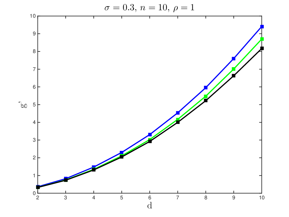
For , Figure 1 shows upper bounds on the gap between the optimal value and the value of the objective function obtained by two methods – Algorithm 5, green curve, and Algorithm 8, blue curve. In Algorithm 8, the initial states are given by the solution to Algorithm 5. The ODE in (20) is solved numerically in Matlab by ode45. For each number of coordinate systems , 100 simulations are conducted and averages are shown in Figure 1. In each simulation a set of transitively consistent orthogonal matrices are generated from a set of orthogonal matrices according to the description in Section 5.1 below. The graph used in each of the experiments is the complete graph.
For a single numerical experiment, Figure 2 shows the improvement of when Algorithm 8 is used. One can see that Algorithm 5 generates matrices that are close to a local optimum of problem (P2).
It can be seen that only a marginal improvement can be made using the significantly more computationally expensive Algorithm 8. Due to the heavy computational burden, in the following simulations we omit Algorithm 8 and focus on the methods based on the Z- and H-matrix.


5.3 Centralized methods for matrices in
In this set of experiments we compare the H-matrix method, the Z-matrix method and a (naive) reference-based method, where the latter serves as baseline for the comparison.
5.3.1 The reference-based method
For the reference-based method, a minimum QSC graph with edges is randomly drawn as a subgraph of . For that, all centers (see Def. 2) of the graph are initially determined by looking at the distance matrix between all nodes. From the set of centers, a node is randomly selected. Since is QSC, there is at least one such center. Let be the list of nodes that have already been considered and initialise . The following procedure is repeated until : randomly select a node , select a random node , if there is such an , add the edge to and add to .
Per construction, the graph is a spanning tree that contains a center. Thus, according to Lemma 12, the set is transitively consistent for . W.l.o.g., by setting for the center of , all (other) are (uniquely) determined as
| (22) |
To summarise, in the reference-based method a (random) rooted spanning tree graph is considered as subgraph of , i.e., all but relative transformations (accounting for the transitive inconsistency) are discarded such that the remaining relative transformations are transitively consistent.
In Fig. 3 the results of the experiments are shown. On the vertical axis, a normalised version of the function in (8), defined by
| (23) |
is used. Each sub-figure shows a different varying parameter on the horizontal axis. The title of each sub-figure indicates the fixed parameters.
It can be seen that in all cases the Z-matrix approach is nearly as good as the H-matrix approach when looking at orthogonal transformations. However, as anticipated, the reference-based method performs worse than both proposed methods. For the case of different degrees of noise (Fig. 3, top left) it can be seen that the total error increases with increasing noise. Similarly, in the case of different dimensions (Fig. 3, bottom left), the error increases with increasing dimensionality. This can be explained by the fact that the Frobenius norm in (23) sums over values. For various values of the graph density (Fig. 3, top right), the error for the H- and Z-matrix method is approximately constant (apart from the case of a rooted spanning tree at , according to Lemma 12.).
5.4 Centralized methods for matrices in
In this set of experiments we compare the H-matrix method and the Z-matrix method.
Using the reference-based method for the case of linear transformations is problematic because this method inverts the matrices for (see (23)). Therefore, for reasonably large noise, it is likely that there is some where is ill-conditioned, resulting in the corresponding term in blowing up. In Fig. 5 this problem is illustrated, where the horizontal axis is shown in log-scale. The lines of the Z- and H-matrix methods almost coincide, so only the green line of the H-matrix method is visible. The reference-based method’s (black) line results in extremely large errors. Due to this reason, and since we have already shown that for the case of orthogonal transformations the reference-based method is inferior, in the following the reference based method is not used in the comparisons.
For the complete graph case, in Figure 7 the improved performance the Gauss-Newton method, i.e., Algorithm 3, (with the solution of the -matrix method as initialization) is shown. The Gauss-Newton method run 5 iterations, but from inspection it could be deduced that the main convergence occurs already after two iterations.
In Fig. 6, the comparisons of the -matrix method and the -matrix method are shown. It can be seen that for small noise (Fig. 6, top left) both methods are comparable, whereas for a larger amount of noise the H-matrix method is able to obtain a smaller error. Similarly, for transformations with small dimensionality (Fig. 6, bottom left), both methods are comparable whereas for larger dimensions the gap between both approaches increases. On the contrary, (Fig. 6, top right) illustrates that with increasing graph density the line of the Z-matrix method approaches that of the H-matrix method (apart from the spanning tree case when , analogous to the orthogonal transformation experiments). This indicates that the H-matrix method performs better than the Z-matrix method if there is only little information available. A similar observation can be made for various (Fig. 6, bottom right). For each subfigure, 100 simulations for a certain configuration of , , , and are shown.
5.5 Methods for affine and Euclidean transformations
In Figure 8 – for affine and Euclidean transformations – a comparison between four different methods can be found. The transformations are affine respective Euclidean, but only the Algorithm 4 methods (red and black) preserve this property. In the bottom right figure the transformations obtained in the -matrix method respective the -matrix method have been projected onto , i.e., the set of Euclidean transformations. The orthogonal matrix part of the transformations were generated according to the description above. The elements in the transnational vectors were drawn from the uniform distribution over and additional element-wise noise was added.


5.6 Distributed methods
Results of the distributed Z-matrix method are shown in Fig. 9 and results for the distributed H-matrix method are shown in Fig. 10.
Conclusions
This worked addressed transitive consistency of linear inverible transformations between Euclidean coordinate systems. Given a set of linear invertible transformations (or matrices) – that are not transitively consistent – the proposed methods synchronize the transformations. This means that they provide transformations that are both transitively consistent and close to the original non-synchronized transformations. First two different direct or centralized approaches were proposed. In the first approach – the -matrix approach – linear algebraic conditions were formulated that must hold for transitively consistent transformations. Then the sought transformations are obtained from the solution of a least squares problem. In the second approach – the -matrix approach – optimization problems were formulated directly, without taking a detour via linear algebraic constraints. The sought transformations are obtained from the solution of the optimization problems.
A Gauss-Newton iterative method was also proposed where the solution from the -matrix method was used as initialization. This method was later adapted to the case of affine and Euclidean transformations. It was shown in numerical simulations that for the case of affine and Euclidean transformations, this approach outperforms the -matrix approach and the -matrix approach. However, for orthogonal transformations no improvement is possible over the -matrix method.
In a later part of the paper, for orthogonal matrices, two distributed algorithms were presented. These algorithms share similarities with linear consensus algorithms for distributed averaging. It was shown that these simple consensus-like protocols can be used to provide a solution to our problem that is very close to the global optimum – even for noise large in magnitude. The proposed methods – both the direct/centralized and the iterative/distributed – have been verified to work in numerical experiments for a wide range of parameter settings.
References
- [1] R. Tron and R. Vidal. Distributed 3-d localization of camera sensor networks from 2-d image measurements. Transactions on Automatic Control, 59(12):3325–3340, 2014.
- [2] V. Lepetit, F. Moreno-Noguer, and P. Fua. Epnp: An accurate o (n) solution to the pnp problem. International journal of computer vision, 81(2):155–166, 2009.
- [3] O. Škrinjar, A. Bistoquet, and H. Tagare. Symmetric and transitive registration of image sequences. Journal of Biomedical Imaging, 2008:14, 2008.
- [4] S. Joshi, B. Davis, M. Jomier, and G. Gerig. Unbiased diffeomorphic atlas construction for computational anatomy. NeuroImage, 23:S151–S160, 2004.
- [5] T.F. Cootes, S. Marsland, C.J. Twining, K. Smith, and C.J. Taylor. Groupwise diffeomorphic non-rigid registration for automatic model building. In Computer Vision-ECCV 2004, pages 316–327. Springer, 2004.
- [6] S. Allassonnière, Y. Amit, and A. Trouvé. Towards a coherent statistical framework for dense deformable template estimation. Journal of the Royal Statistical Society: Series B (Statistical Methodology), 69(1):3–29, 2007.
- [7] F. Bernard, J. Thunberg, A. Husch, L. Salamanca, P. Gemmar, F. Hertel, and J. Goncalves. Transitively consistent and unbiased multi-image registration using numerically stable transformation synchronisation. In Workshop on Spectral Analysis in Medical Imaging (SAMI), to appear. MICCAI, 2015.
- [8] T. Gass, G. Szekely, and O. Goksel. Detection and correction of inconsistency-based errors in non-rigid registration. In SPIE Medical Imaging, pages 90341B–90341B. International Society for Optics and Photonics, 2014.
- [9] X. Geng. Transitive inverse-consistent image registration and evaluation. ProQuest, 2007.
- [10] J.C. Gower and G.B. Dijksterhuis. Procrustes problems, volume 3. Oxford University Press Oxford, 2004.
- [11] K.S. Arun, T.S. Huang, and S.D. Blostein. Least-squares fitting of two 3-D point sets. IEEE Transactions on Pattern Analysis and Machine Intelligence, (5):698–700, 1987.
- [12] P.H. Schönemann. A generalized solution of the orthogonal procrustes problem. Psychometrika, 31(1):1–10, March 1966.
- [13] B.K.P. Horn, H.M. Hilden, and S. Negahdaripour. Closed-form solution of absolute orientation using orthonormal matrices. Journal of the Optical Society of America A, 5(7):1127, 1988.
- [14] B.K.P. Horn. Closed-form solution of absolute orientation using unit quaternions. Journal of the Optical Society of America A, 4(4):629–642, 1987.
- [15] M.W. Walker, L. Shao, and R.A. Volz. Estimating 3-D location parameters using dual number quaternions. CVGIP: Image Understanding, 54(3):358–367, November 1991.
- [16] D. Pizarro and A. Bartoli. Global optimization for optimal generalized procrustes analysis. In Computer Vision and Pattern Recognition (CVPR), 2011 IEEE Conference on, pages 2409–2415. IEEE, 2011.
- [17] F. Bernard, J. Thunberg, P. Gemmar, F. Hertel, A. Husch, and J. Goncalves. A solution for multi-alignment by transformation synchronisation. In Conference on Computer Vision and Pattern Recognition. IEEE, 2015.
- [18] A. Singer and Y. Shkolnisky. Three-Dimensional Structure Determination from Common Lines in Cryo-EM by Eigenvectors and Semidefinite Programming. SIAM journal on imaging sciences, 4(2):543–572, June 2011.
- [19] R. Hadani and A. Singer. Representation Theoretic Patterns in Three-Dimensional Cryo-Electron Microscopy II—The Class Averaging Problem. Foundations of computational mathematics (New York, N.Y.), 11(5):589–616, 2011.
- [20] R. Hadani and A. Singer. Representation theoretic patterns in three dimensional Cryo-Electron Microscopy I: The intrinsic reconstitution algorithm. Annals of mathematics, 174(2):1219, 2011.
- [21] K.N. Chaudhury, Y. Khoo, and A. Singer. Global registration of multiple point clouds using semidefinite programming. arXiv.org, June 2013.
- [22] D. Pachauri, R. Kondor, and V. Singh. Solving the multi-way matching problem by permutation synchronization. In Advances in neural information processing systems, pages 1860–1868, 2013.
- [23] J. Thunberg, F. Bernard, and J. Goncalves. Centralized and distributed transformation synchronization under partial information. Submitted to: Transactions on Pattern Analysis and Machine Intelligence.
- [24] M. Mesbahi and M. Egerstedt. Graph theoretic methods in multiagent networks. Princeton University Press, 2010.
- [25] A. Jadbabaie and A. S. Morse. Coordination of groups of mobile autonomous agents using nearest neighbor rules. IEEE Transactions on Automatic Control, 48(6):988–1001, 2003.
- [26] R. Olfati-Saber and R. Murray. Consensus problems in networks of agents with switching topology and time-delays. IEEE Transactions on Automatic Control, 49(9):1520–1533, 2004.
- [27] R. Olfati-Saber, J.A. Fax, and R.M. Murray. Consensus and cooperation in networked multi-agent systems. Proceedings of the IEEE, 95(1):215–233, 2007.
- [28] R. Olfati-Saber and R. M. Murray. Consensus problems in networks of agents with switching topology and time-delays. IEEE Transactions on Automatic Control, 49(9):1520–1533, 2004.
- [29] J. Thunberg. Consensus and Pursuit-Evasion in Nonlinear Multi-Agent Systems. PhD thesis, KTH Royal Institute of Technology, 2014.
- [30] T. Yoshizawa. Stability theory by Liapunov’s second method. Mathematical Society of Japan (Tokyo), 1966.
- [31] F.H. Clarke. Generalized gradients and applications. Transactions of the American Mathematical Society, 205:247–262, 1975.
- [32] G. Shi and Y. Hong. Global target aggregation and state agreement of nonlinear multi-agent systems with switching topologies. Automatica, 45(5):1165–1175, 2009.
- [33] Z. Lin, B. Francis, and M. Maggiore. State agreement for continuous-time coupled nonlinear systems. SIAM Journal on Control and Optimization, 46(1):288–307, 2007.
- [34] H. K. Khalil. Nonlinear systems, volume Third Edition. Prentice hall, 2002.
- [35] Nicholas J Higham. Functions of matrices: theory and computation. Siam, 2008.
- [36] D.G. Luenberger. Introduction to linear and nonlinear programming, volume 28. Addison-Wesley Reading, MA, 1973.
- [37] A. Forsgren and T. Odland. On the connection between the conjugate gradient method and quasi-newton methods on quadratic problems. Computational optimization and applications, 60(2):377–392, 2015.
- [38] A. Lindquist and J. Sand. An introduction to mathematical systems theory. KTH Lecture Notes, Division of Optimization and Systems Theory, Royal Institute of Technology (KTH), 1996.
- [39] B. Afsari. Riemannian Lp center of mass: Existence, uniqueness and convexity. In Proc. Amer. Math. Soc, volume 139, pages 655–673, 2011.
- [40] B. Afsari and P.S. Krishnaprasad. Some gradient based joint diagonalization methods for ica. In Independent Component Analysis and Blind Signal Separation, pages 437–444. Springer, 2004.
- [41] A. Sarlette, R. Sepulchre, and N.E. Leonard. Autonomous rigid body attitude synchronization. Automatica, 45(2):572–577, 2009.