Improved bounded-strength decoupling schemes for local Hamiltonians

Consider a quantum system of $n$ interacting $d$-dimensional qudits with a time-independent (possibly unknown) Hamiltonian $H$ acting on a Hilbert space ${\cal H}\cong({\mathbb{C}}^{d})^{\otimes n}$. We make the assumption that the system is $\ell$-local, i.e. that $H$ can be written as the sum of operators, each of which acts only on $\ell$ of the $n$ qudits. In nature it is usually the case that $\ell$ is small even when $n$ is large. Without loss of generality, we also take $H$ to be traceless, and for technical reasons, we assume that $d$ is a prime power (which includes the important case of qubits, i.e. $d=2$).

We consider the task of decoupling, i.e. effectively switching off the Hamiltonian $H$ (including removing any couplings to the environment) so that the system effectively evolves under the zero Hamiltonian. Such a task is important, for example, in the context of quantum memory, where one desires to preserve the state of a quantum system.

To achieve this task, we assume that the natural dynamics of the system can be modified by adjoining an open-loop (non-feedback) controller according to

In practice, physical limitations restrict the types of control Hamiltonians available for use. We consider the realistic setting in which $H_{c}(t)$ is only 1-local, i.e. due to our limited control of the system, $H_{c}$ is the sum of operators that each act on only one qudit. We further impose the constraint that our control Hamiltonian $H_{c}(t)$ is limited to be bounded-strength, i.e. a sufficiently smooth bounded function. This is in contrast to the setting of bang-bang control in which $H_{c}(t)$ can be a discontinuous function that takes values of arbitrarily large norm. Our assumptions that the system Hamiltonian is an $\ell$-local Hamiltonian acting on a system of $n$ interacting qudits and that the control Hamiltonian is a $1$-local bounded-strength Hamiltonian reflect the typical composite nature of quantum systems and their coupling locality as well as the limitations in implementing external controls.

Viola and Knill proposed a general method for bounded-strength decoupling; see [1] and [2, Chapter 4]. Their method, often referred to as Eulerian decoupling, relies on Eulerian cycles in Cayley graphs of a control group — a certain finite group of control unitaries that can be implemented by switching on control Hamiltonians, from a finite set of available control operations, for a fixed time. The Eulerian cycle dictates which control Hamiltonians are applied in the different time-slots of the decoupling protocol.

The Eulerian method, as introduced in [1], does not make it possible to directly leverage the fact that the system Hamiltonian is $\ell$-local in order to obtain more efficient decoupling schemes. However, in the setting of bang-bang control there do exist efficient decoupling schemes that are specifically designed for composite quantum systems with $\ell$-local system Hamiltonians; see [3, 4, 5] and [2, Chapter 15]. In these schemes, the specification of which bang-bang control unitaries are to be applied is chosen according to the entries of so-called orthogonal arrays of strength $\ell$. They are matrices with the property that any submatrix formed by an arbitrary collection of $\ell$ rows satisfies a certain balancedness condition.

The work [6] presented a particular construction of decoupling schemes merging the approaches of Eulerian (bounded-strength) decoupling together with orthogonal array (bang-bang) decoupling. This construction yields schemes that require only bounded-strength controls and exploit the composite structure of the quantum system (namely, the locality of the system Hamiltonian) to achieve decoupling with fewer control operations. To do so, these schemes introduce the concept of so-called Eulerian orthogonal arrays.

The purpose of the present paper is to further improve upon the method of [6] to obtain even more efficient bounded-strength decoupling schemes. To this end, we first generalize the Eulerian method due to [1] by showing that it is also possible to achieve decoupling with the help of so-called balanced cycles, which encompass Eulerian cycles as a special case. We then show that bounded-strength decoupling of composite quantum systems with local Hamiltonians can be accomplished based on the new concept of balanced-cycle orthogonal arrays.

Note that all the schemes discussed above can also be applied to the situation of a general open quantum system with joint Hamiltonian $H$ acting on a quantum system that is coupled to an uncontrollable environment. Such a Hamiltonian has the form

where the operators $H_{S}$ and $S_{\alpha}$ act on the system and where the operators $H_{B}$ and $B_{\alpha}$ act on the environment. We assume that the system Hamiltonian $H_{S}$ and the operators $S_{\alpha}$ are all $\ell$-local. The decoupling goal in this case is to effectively switch off the system Hamiltonian $H_{S}$ and remove all couplings to the environment. If, using controls that act only on the system, one can effectively switch off all generic system Hamiltonians, then such an operation will switch off $H_{S}$ and each $S_{\alpha}$, thereby accomplishing decoupling.¹¹ 1 The remaining Hamiltonian term of $\id_{S}\otimes H_{B}$ is inconsequential, as it does not affect the system at all. For notational simplicity, the remainder of the paper will therefore ignore the environment and treat only the case of effectively switching off an arbitrary $\ell$-local operator $H$.

Consider the group $({\mathbb{F}}_{q},+)$, the additive group of the finite field of order $q=d^{2}$, where $d$ (the dimension of the qudits) is some prime power. For the remainder of this paper, let $\rho:{\mathbb{F}}_{q}\rightarrow{\mathcal{U}}(d)$ be a faithful, irreducible, unitary, projective²² 2 Projective representations need only be homomorphisms up to phase, i.e. obey $U_{g+h}\propto U_{g}U_{h}$ with proportionality rather than equality. representation that maps the elements of ${\mathbb{F}}_{q}$ to $d\times d$ unitary matrices, say $\rho:g\mapsto U_{g}$. That $q$ cannot be smaller than $d^{2}$ for such a representation will be justified later in Remark 2; that $q=d^{2}$ suffices is justified by the explicit example shown below.

We assume that for every $g\in{\mathbb{F}}_{q}$ we can implement $U_{g}$ on any qudit of our system in the following sense: for every $g$, we can physically implement, over time $\delta\in[0,\Delta]$, a bounded-strength single-qudit Hamiltonian $h_{g}(\delta)$, corresponding to a single-qudit unitary evolution operator $u_{g}(\delta)$, such that $U_{g}=u_{g}(\Delta)$ where $\Delta$ is some fixed length of time. We assume that we can do this on any qudit and, moreover, that we can do so for each of the $n$ qudits in parallel. Note that this assumption obeys the practical control limitations discussed earlier.

Of particular interest, in the case of qubits ($d=2,q=4$) we can consider the representation $\rho:{\mathbb{F}}_{4}\rightarrow{\mathcal{U}}(2)$ that maps the four elements of ${\mathbb{F}}_{4}$ to the four $2\times 2$ Pauli matrices $\{\id,X,Y,Z\}$. Thus, it is assumed that we can physically implement any Pauli operator on any qubit. Rather than assuming that $q=4$, this paper will treat $q$ more generally; however the reader is invited to think of the special case of qubits if desired. For non-qubits, with $q>4$, we can generalize this example as follows. For a prime $p$, define $\tilde{X}=\sum_{j=0}^{p-1}|j+1\text{ mod }p\rangle\langle j|$ and $\tilde{Z}=\sum_{j=0}^{p-1}\omega^{j}|j\rangle\langle j|$, where $\omega$ is a $p^{\text{th}}$ root of unity. For prime $d=p$, the map $(a,b)\mapsto\tilde{X}^{a}\tilde{Z}^{b}$ defines a faithful, irreducible, unitary, projective representation from ${\mathbb{Z}}_{d}\times{\mathbb{Z}}_{d}$ to ${\mathcal{U}}(d)$. For a prime power $d=p^{e}$ (for some $e$), map $((a_{1},b_{1}),\ldots,(a_{e},b_{e}))\mapsto\tilde{X}^{a_{1}}\tilde{Z}^{b_{1}}\otimes\cdots\otimes\tilde{X}^{a_{e}}\tilde{Z}^{b_{e}}$.

A decoupling protocol is defined by specifying a sequence of control Hamiltonians (equivalently, control unitaries) to be applied. As shown in Fig. 1, we construct an $n\times N$ array with entries from ${\mathbb{F}}_{q}$, which we regard as a sequence of $N$ columns from ${\mathbb{F}}_{q}^{n}$. The $j$th column $\vec{g}_{j}=(g_{1j},\ldots,g_{nj})^{T}$ corresponds to the $j$th time interval $\big[(j-1)\Delta,j\Delta\big]$ of our protocol, during which we apply the control Hamiltonian

that gives rise to evolution $u_{\vec{g}_{j}}(\delta)=u_{g_{1j}}(\delta)\otimes\cdots\otimes u_{g_{nj}}(\delta)$ over $\delta\in[0,\Delta]$. In other words, for each $\delta\in[0,\Delta]$ and $j=1,\ldots,N$, $H_{c}(t)=h_{\vec{g}_{j}}(\delta)$ where $t=(j-1)\Delta+\delta$. The total time required to apply the entire sequence, i.e. the control cycle length, is therefore $T_{c}=N\Delta$, at which point the control sequence can be repeated. Observe that for any $t=(j-1)\Delta+\delta$, the unitary evolution $U_{c}(t)$ corresponding to the control Hamiltonian consequently satisfies $U_{c}(t)=u_{\vec{g}_{j}}(\delta)U_{c}\big((j-1)\Delta\big)$.

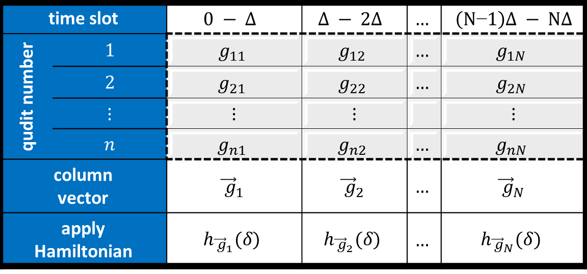
According to average Hamiltonian theory [7, 8, 9], the resulting system evolution under $H+H_{c}(t)$ can be effectively approximated by

at times $t$ that are integer multiples of $T_{c}$, i.e. $t=mT_{c}$ for any $m\in{\mathbb{N}}$, where

is time-independent and where $U_{c}(t)$ is the time evolution due to $H_{c}(t)$ alone. The goal of decoupling, therefore, is to choose $U_{c}(t)$ such that $\bar{H}^{(0)}=0$ for any $H$. It is in this sense that we effectively switch off the Hamiltonian $H$. We refer the reader to [10] for a detailed description of the above control-theoretic model and the resulting effective time-evolution. We note, in particular, that although the approximation above is to leading order (in the Magnus expansion of $U_{c}(t)^{\dagger}HU_{c}(t)$), the second-order term may be eliminated by designing the control Hamiltonian to satisfy $U_{c}(t)=U_{c}(T_{c}-t)$ [9].

The efficiency of the protocol developed in this paper is obtained by exploiting the composite structure of the Hamiltonian, namely the fact that $H$ was assumed to be a local Hamiltonian. By definition, an $\ell$-local Hamiltonian $H$ on $n$ qudits can be written as $H=\sum_{k}H_{k}$, where each $H_{k}$ acts non-trivially on at most $\ell$ of the $n$ qudits. In particular, the $\ell=2$ case corresponds to Hamiltonians with only pairwise interactions. Our goal is to create a protocol that decouples each $H_{k}$ simultaneously, and therefore decouples $H$. To see that this would work, observe that for any protocol $U_{c}(t)$,

The success of the decoupling protocol introduced in this paper will rely on some basic group theory, which we introduce now. Let ${\mathcal{G}}$ be an Abelian group with a generating set ${\mathscr{S}}\subset{\mathcal{G}}$, i.e. any element of ${\mathcal{G}}$ can be written as a sum of elements from ${\mathscr{S}}$.

Note that a cycle may visit vertices more than once and may traverse edges multiple times. We will be interested not only in the vertices, but also the specific labels leaving each vertex; we denote by ${\text{\footnotesize g}}\bullet\!\!\!\xrightarrow{{\text{\footnotesize s}}}$ the s-labeled edge leaving vertex g.

An important special case of a balanced cycle is an Eulerian cycle on $\Gamma({\mathcal{G}},{\mathscr{S}})$, for which $\mu_{\text{\footnotesize s}}=1$ for every ${\text{\footnotesize s}}\in{\mathscr{S}}$. Examples of an Eulerian cycle and a non-Eulerian balanced cycle are shown in Fig. 2(a) and Fig. 2(b) respectively. In [1], Eulerian cycles were used to define decoupling protocols that avoided the discontinuous nature of bang-bang decoupling. More generally, one can define decoupling protocols based on balanced cycles (of which Eulerian decoupling is a special case), to which we now turn our attention. Note, however, that this balanced-cycle decoupling protocol will not be the goal of this paper. Indeed, such a protocol will not exploit the composite structure of the Hamiltonian. Later we will utilize the balanced-cycle decoupling on $\ell$-qudit subsystems of a larger $n$ qudit space to develop more efficient protocols; in the current section, however, we may regard $\ell$ as the size of the entire system.

In exploiting the $\ell$-local nature of $H$, we will find that we are primarily interested in the group

with some generating set ${\mathscr{S}}$ and the representation

defined from our representation $\rho:{\mathbb{F}}_{q}\rightarrow{\mathcal{U}}(d)$. Specifically, if ${\text{\footnotesize g}}=(a_{1},\ldots,a_{\ell})^{T}\in{\mathcal{G}}$ and $\rho(a_{i})=U_{a_{i}}$ then $\rho^{\otimes\ell}({\text{\footnotesize g}})=U_{\text{\footnotesize g}}=U_{a_{1}}\otimes\cdots\otimes U_{a_{\ell}}$. By our assumptions above, we can physically implement $U_{\text{\footnotesize g}}$ by applying the control unitary $u_{\text{\footnotesize g}}(\delta)$ (equivalently, the control Hamiltonian $h_{\text{\footnotesize g}}(\delta)$) for time $\Delta$. For example, in the case of qubits ($q=4$), the group ${\mathbb{F}}_{4}$, whose elements we denote³³ 3 Here the reader may prefer to equivalently think of the Abelian group as $\{1,z,x,y=xz=zx\}$ with generating set $S_{4}=\{z,x\}$. Then we can use ${\mathscr{S}}=\{z^{(1)},x^{(1)},\ldots z^{(\ell)},x^{(\ell)}\}$ and $\rho(x)=X,\rho(y)=Y,$ and $\rho(z)=Z$. Be aware, however, that the group operation used throughout the paper is denoted by $+$ rather than by multiplication, since it is inherited from the finite field. as $\{0,1,\alpha,\alpha+1\}$, is generated by the set $S_{4}=\{1,\alpha\}$. We choose ${\mathscr{S}}=\{1^{1},\alpha^{1},\ldots 1^{\ell},\alpha^{\ell}\}$, which is a generating set of $2\ell$ elements for the group ${\mathcal{G}}={\mathbb{F}}_{4}^{\ell}$, where $x^{i}$ here denotes the column $(0,\ldots,0,x,0,\ldots,0)^{T}$ with $x\in{\mathbb{F}}_{q}$ in the $i$th position. In this case we assume $\rho(a_{i})=U_{a_{i}}$ is a Pauli matrix, so $\rho^{\otimes\ell}({\text{\footnotesize g}})$ is a tensor product of Pauli matrices.

The purpose for the group theory used in this paper resides in the following observation [2, Chapter 4]. We define the operator $\Pi_{\mathcal{G}}$ to act on matrices $A$ as

Note that for every matrix $A$, $\Pi_{\mathcal{G}}(A)$ commutes with all $U_{\text{\footnotesize g}}$ (${\text{\footnotesize g}}\in{\mathcal{G}}$). Thus, by Schur’s lemma, since $\rho$ is irreducible⁴⁴ 4 Schur’s lemma guarantees this directly when $\ell=1$. But then it also applies for $\ell=2$ since then for any matrix $A=\sum_{i}B_{i}\otimes C_{i}$, we have $\Pi_{\mathcal{G}}(A)=\frac{1}{|{\mathcal{G}}|}\sum_{i}\sum_{a_{1},a_{2}\in{\mathbb{F}}_{q}}U_{a_{1}}^{\dagger}B_{i}U_{a_{1}}\otimes U_{a_{2}}^{\dagger}C_{i}U_{a_{2}}\propto\sum_{i}{\rm tr}{B_{i}}{\rm tr}{C_{i}}={\rm tr}{\sum_{i}B_{i}\otimes C_{i}}={\rm tr}{A}$, and similarly for larger $\ell$. , we have $\Pi_{\mathcal{G}}(A)=\frac{{\rm tr}(A)}{D}\id$ (where $D$ is the dimension of the Hilbert space). In particular then, if ${\rm tr}(A)=0$ then $\Pi_{\mathcal{G}}(A)=0$.

Observe that the key to this protocol working is the fact that each $u_{\text{\footnotesize s}}(\delta)U_{\text{\footnotesize g}}$ shows up an equal number of times, independent of g, i.e. $\forall{\text{\footnotesize s}}\in{\mathscr{S}}\ \exists\mu_{s}>0$ such that $\forall{\text{\footnotesize g}}\in{\mathcal{G}},\ {\text{\footnotesize g}}\bullet\!\!\!\xrightarrow{{\text{\footnotesize s}}}$ occurs $\mu_{\text{\footnotesize s}}$ times (independent of g). In an Eulerian cycle, $\mu_{\text{\footnotesize s}}=1$ for every s, which is certainly sufficient. All else being equal, given the choice between Eulerian and other balanced cycles, we would choose Eulerian cycles as they will minimize $N$ and therefore $T_{c}$. However, we will see that when considering the composite properties of a system (specifically that interactions are local), we will be able to exploit the notion of balanced cycles to come up with a much more efficient protocol.

In Section II and Fig. 1, we indicated how we view our decoupling scheme as an array. For the protocol to be efficient, we shall ensure that this array corresponds to what we call a balanced-cycle orthogonal array (BOA). A BOA is a special type of orthogonal array (OA), which we first define. We refer the reader to [11] for a thorough introduction to OAs, particularly their relationship to linear codes (of which we shall later make use).

For notational consistency, we point out that throughout the remainder of this paper we adopt the notation that ${\mathcal{G}}$ and ${\mathscr{S}}$ refer specifically to the group ${\mathbb{F}}_{q}^{\ell}$ and a generating set for ${\mathbb{F}}_{q}^{\ell}$, respectively. Elements of ${\mathcal{G}}$ will be denoted using script g, elements of ${\mathscr{S}}$ will be denoted using script s, and cycles on ${\mathcal{G}}$ will be denoted L. When other groups (such as ${\mathbb{F}}_{q}$ or ${\mathbb{F}}_{q}^{n}$) are being considered, other notation (such as $g$, $m$, $S$, $s$ and ${\mathcal{L}}$) will be used instead.

An example of an $OA_{2}(8,7,2,2)$ is shown in Fig. 3. Orthogonal arrays have been used to construct bang-bang decoupling schemes (see [3, 4, 5] and [2, Chapter 15]). In order to construct a bounded-strength scheme, we introduce the notion of a balanced-cycle orthogonal array, defined as follows.

An example of a BOA is shown in Fig. 4. We defer the proof that BOAs exist to Sec. V. The remainder of the current section defines a decoupling protocol based on BOAs and proves that it works to decouple $\ell$-local Hamiltonians in $n$ qudit systems ($\ell\leqslant n$). Working with $\ell$ qudits (rather than $n$ qudits), along with the promise that $H$ is $\ell$-local, will enable us to give an efficient protocol.

Theorem 2 showed that decoupling protocols based on BOAs work, with control cycle length proportional to the BOA parameter $N$. We next show that BOAs can indeed be constructed and, moreover, that the construction gives rise to an efficient decoupling protocol, in the sense that $N$ does not increase exponentially with $n$.

The existence of balanced-cycle orthogonal arrays follows naturally from constructions of orthogonal arrays generated using classical linear codes, which we shall define shortly. We first give a brief outline of our BOA construction. This construction is via the generator matrix $G$ of a linear code, which is a linear mapping from ${\mathbb{F}}_{q}^{k}$ to ${\mathbb{F}}_{q}^{n}$ for some $k\leqslant n$. If we enumerate all elements of ${\mathbb{F}}_{q}^{k}$ in an arbitrary order and consider their image under $G$, this will form an OA of strength $\ell$ (for an appropriately chosen $k$). To obtain a BOA, we do this enumeration according to the prescription of an Eulerian cycle on ${\mathbb{F}}_{q}^{k}$. In doing so, we can guarantee that we always obtain a balanced cycle when we consider any submatrix of $\ell$ rows, ultimately ensuring that any $\ell$-local Hamiltonian term on those corresponding qudits will be decoupled. We now prove this, starting with a definition of a classical linear code.

The dual code $C^{\perp}$ of $C$ is defined by $C^{\perp}=\{y\in{\mathbb{F}}_{q}^{n}:x\cdot y=0\ \forall x\in C\}$ with the dot product $x\cdot y=\sum_{i=1}^{n}x_{i}y_{i}$. The dual code is also a classical linear code, namely an $[n,n-k]_{q}$ code with some distance $\delta^{\perp}$ that we will refer to as the dual distance. Orthogonal arrays can be constructed from linear codes, as the following theorem [11, Theorem 4.6] establishes.

Let $C$ be an $[n,k]_{q}$ with dual distance $\delta^{\perp}=\ell+1$ and generating matrix $G$. Let ${\mathcal{L}}$ be an Eulerian cycle on the Cayley graph $\Gamma({\mathbb{F}}_{q}^{k},S_{q}^{(k)})$, where $S_{q}^{(k)}$ is a generating set for ${\mathbb{F}}_{q}^{k}$; thus, we can write ${\mathcal{L}}_{{\mathbb{F}}_{q}^{k}}=(m_{0},\ldots,m_{N-1})$ with transitions ${\mathcal{L}}_{S_{q}^{(k)}}=(s_{1},\ldots,s_{N})$ and $N=q^{k}\,|S_{q}^{(k)}|$. Because $d$ is a prime power, say $d=p^{e}$ for some prime $p$, the minimal generating set is of size $|S_{q}^{(k)}|=2ke$. We are interested in the image of the cycle in the codespace; thus, consider the Eulerian cycle, denoted $G{\mathcal{L}}$, on $\Gamma(G[{\mathbb{F}}_{q}^{k}],G[S_{q}^{(k)}])$, where $G[{\mathbb{F}}_{q}^{k}]=C\subset{\mathbb{F}}_{q}^{n}$ is the image of ${\mathbb{F}}_{q}^{k}$ under $G$, i.e. is the codespace. In other words, $G{\mathcal{L}}_{{\mathbb{F}}_{q}^{k}}=(Gm_{0},\ldots,Gm_{N-1})$ and $G{\mathcal{L}}_{S_{q}^{(k)}}=(Gs_{1},\ldots,Gs_{N})$.

To avoid possible confusion, we emphasize here that although we will use $G{\mathcal{L}}$ to construct a BOA, neither ${\mathcal{L}}$ nor $G{\mathcal{L}}$ will serve as the balanced cycle to which Theorem 1 applies (which is why we have used the notation ${\mathcal{L}}$ rather than L). Rather, for our efficient decoupling scheme, we construct an array $A_{G{\mathcal{L}}}$, dictated by $G{\mathcal{L}}$, and prove that the result is a BOA by showing that if we consider any subarray of $\ell$ rows, it gives rise to some balanced cycle L on ${\mathcal{G}}={\mathbb{F}}_{q}^{\ell}$. The notation and relationships of the various groups and cycles used in this paper is sketched in Fig. 5.

We turn $G{\mathcal{L}}$ into an array $A_{G{\mathcal{L}}}$ in the obvious way as follows. Each element $Gm_{j}$ of $G{\mathcal{L}}_{{\mathbb{F}}_{q}^{k}}$ is a column vector in ${\mathbb{F}}_{q}^{n}$. Therefore we may associate to $G{\mathcal{L}}$ the $n\times N$ matrix $A_{G{\mathcal{L}}}=[Gm]_{m\in{\mathcal{L}}_{{\mathbb{F}}_{q}^{k}}}$ with elements $a_{ij}=(Gm_{j})_{i}$, so that the $j$th column of $A_{G{\mathcal{L}}}$ is the vector $Gm_{j}$, and the columns are arranged in the order of the Eulerian cycle $G{\mathcal{L}}$. Note that since we assumed that Eulerian cycles always start with the (additive) identity element, i.e. the zero vector $o\in{\mathbb{F}}_{q}^{k}$, and since $G$ maps the zero vector to the zero vector ($Go=o\in{\mathbb{F}}_{q}^{n}$), the first column of $A_{G{\mathcal{L}}}$ is the zero vector of ${\mathbb{F}}_{q}^{n}$.

Let $s\in S_{q}^{(k)}$. $Gs\in{\mathbb{F}}_{q}^{n}$, so $Gs=\Big((Gs)_{1},\ldots,(Gs)_{n}\Big)^{T}$, where we use the notation $(Gs)_{i}\in{\mathbb{F}}_{q}$ to denote the $i$th component of the column vector $Gs$. Fix $\ell$ distinct numbers $i_{1},\ldots,i_{\ell}\in\{1,\ldots,n\}$ and write $I=\{i_{1},\ldots,i_{\ell}\}$. Let $(Gs)_{I}$ denote the $\ell$-tuple $\Big((Gs)_{i_{1}},\ldots,(Gs)_{i_{\ell}}\Big)^{T}$. Let ${\mathscr{S}}=\left\{(Gs)_{I}:s\in S_{q}^{(k)}\right\}$.

References

- [1] L. Viola and E. Knill, “Robust dynamical decoupling of quantum systems with bounded controls,” Phys. Rev. Lett., vol. 90, p. 037901, 2003. http://link.aps.org/doi/10.1103/PhysRevLett.90.037901
- [2] D. A. Lidar and T. A. Brun, Eds., Quantum error correction. Cambridge University Press, 2013.
- [3] M. Stollsteimer and G. Mahler, “Suppression of arbitrary internal coupling in a quantum register,” Phys. Rev. A, vol. 64, p. 052301, 2001. http://link.aps.org/doi/10.1103/PhysRevA.64.052301
- [4] P. Wocjan, M. Roetteler, D. Janzing, and T. Beth, “Simulating hamiltonians in quantum networks: Efficient schemes and complexity bounds,” Phys. Rev. A, vol. 65, p. 042309, 2002. http://link.aps.org/doi/10.1103/PhysRevA.65.042309
- [5] M. Roetteler and P. Wocjan, “Equivalence of decoupling schemes and orthogonal arrays,” Information Theory, IEEE Transactions on, vol. 52, no. 9, pp. 4171–4181, 2006. http://dx.doi.org/10.1109/TIT.2006.880059
- [6] P. Wocjan, “Efficient decoupling schemes with bounded controls based on eulerian orthogonal arrays,” Phys. Rev. A, vol. 73, p. 062317, 2006. http://link.aps.org/doi/10.1103/PhysRevA.73.062317
- [7] R. R. Ernst, G. Bodenhausen, and A. Wokaun, Principles of nuclear magnetic resonance in one and two dimensions. Clarendon Press Oxford, 1987, vol. 14.
- [8] J. Waugh, L. Huber, and U. Haeberlen, “Approach to high-resolution nmr in solids,” Physical Review Letters, vol. 20, no. 5, pp. 180–182, 1968. http://dx.doi.org/10.1103/PhysRevLett.20.180
- [9] U. Haeberlen, High resolution NMR in solids: Selective averaging, Advances in magnetic resonance: Suppl. 1. Academic Press, 1976, vol. 1.
- [10] A. D. Bookatz, P. Wocjan, and L. Viola, “Hamiltonian quantum simulation with bounded-strength controls,” New Journal of Physics, vol. 16, no. 4, p. 045021, 2014. http://dx.doi.org/10.1088/1367-2630/16/4/045021
- [11] A. S. Hedayat, N. J. A. Sloane, and J. Stufken, Orthogonal arrays: theory and applications. Springer Science & Business Media, 1999.
- [12] M. Roetteler, “Dynamical decoupling schemes derived from Hamilton cycles,” Journal of Mathematical Physics, vol. 49, p. 042106, 2008. http://dx.doi.org/10.1063/1.2904471
- [13] F. J. MacWilliams and N. J. A. Sloane, The Theory of error-correcting codes. North-Holland, 1977.
- [14] S. Lin and D. J. Costello, Error Control Coding. Prentice Hall, 2004.
- [15] R. M. Roth, Introduction to Coding Theory. Cambridge University Press, 2006.
- [16] M. Sudan, 2001, Lecture notes for Algorithmic Introduction to Coding Theory (MIT 6.897). http://people.csail.mit.edu/madhu/FT01/
- [17] S. Yekhanin and I. Dumer, “Long nonbinary codes exceedings the Gilbert-Varshamov bound for any fixed distance,” IEEE Transactions on Information Theory, vol. 50, no. 10, pp. 2357–2362, 2004. http://dx.doi.org/10.1109/TIT.2004.834744
- [18] Y. Edel and J. Bierbrauer, “Large caps in small spaces,” Designs, Codes, and Cryptography, vol. 23, no. 2, pp. 197–212, 2001. http://dx.doi.org/10.1023/A%3A1011216716700
- [19] W. Bosma, J. J. Cannon, and C. Playoust, “The Magma algebra system I: The user language,” Journal of Symbolic Computation, vol. 24, no. 3–4, pp. 235–265, 1997. http://dx.doi.org/10.1006/jsco.1996.0125
- [20] F. R. Kschischang and S. Pasupathy, “Some ternary and quaternary codes and associated sphere packings,” IEEE Trans. Inf. Theory, vol. 38, no. 2, pp. 227–246, 1992. http://dx.doi.org/10.1109/18.119683
- [21] D. Janzing, P. Wocjan, and T. Beth, “Complexity of decoupling and time reversal for n spins with pair interactions: Arrow of time in quantum control,” Phys. Rev. A, vol. 66, p. 042311, 2002. http://link.aps.org/doi/10.1103/PhysRevA.66.042311