Cascade Markov Decision Processes: Theory and Applications

We use the framework of [1] for continuous-time finite-state (FSCT) Markov processes. We assume a probability space $(\Omega,\mathcal{F},\mathbb{P})$ and right-continuous stochastic processes adapted to a filtration $\mathbb{F=(}\mathcal{F}_{t})_{t\in T}$ on this space. An FSCT Markov process $x_{t}$ that is assumed to take values in $\{e_{i}\}_{i=1}^{n}$, the set of $n$standard basis vectors in $\mathbb{R}^{n}$, has the following sample path (Itô) description: descriptions:

$\displaystyle dx$

$\displaystyle=$

$\displaystyle\sum_{i=1}^{m}G_{i}xdN_{i}~~$

(2.1)

where $G_{i}\in\mathbb{G}^{n}$ are distinct¹¹ 1 If the $G_{i}^{\prime}s$ are not distinct, then one can combine the Poisson counters corresponding to identical $G_{i}^{\prime}s$ to get a set of distinct $G_{i}^{\prime}s$. For example, $G_{1}ydN_{1}+G_{1}ydN_{2}$ can be replaced by $G_{1}ydN$ where $dN=dN_{1}+dN_{2},$ a Poisson counter with rate equal sum of the rates of the counters $N_{1},N_{2}$, $\mathbb{G}^{n}$ being the space of square $n-$matrices of the form $F_{kl}-F_{ll}$  where $F_{ij}$ is the matrix of all zeros except for one in the $i^{\prime}th$ row and $j^{\prime}th$ column, and $N_{i}$ are Poisson counters with rates $\lambda_{i}.$ The resulting infinitesimal generator that governs the transition probabilities of the process is $P\in\mathbb{P}^{n}$, the space of all stochastic $n-$matrices and is given by:

$\displaystyle P$

$\displaystyle=$

$\displaystyle\sum_{i=1}^{m}G_{i}\lambda_{i}$

In a Markov decision process, the transition rates are allowed to depend on $\mathcal{F}_{t}-$progressively measurable control processes $u=(u_{1,}u_{2}...u_{p})$ in an affine accordance with²² 2 that is, we assume an affine dependence on controls:

$$\lambda_{i}=\lambda_{i0}+\sum_{j=1}^{p}\mu_{ij}u_{j}$$

so that the infinitesimal generator can be written as:

$$P(u)=\sum_{i=1}^{m}G_{i}\left(\lambda_{i0}+\sum_{j=1}^{p}\mu_{ij}u_{j}\right)$$

We are interested in the case where transition rates of $x_{t}\in\{e_{i}\}_{i=1}^{n}$ are themselves stochastic: specifically, they depend on the state of another Markov process, say, $z_{t}\in\{e_{i}\}_{i=1}^{r}$. We will call such a pair to form a Cascade Markov chain (CMC) In general, various levels of interactions between two processes $x_{t}$ and $z_{t}$ defines a joint Markov process $y_{t}=z_{t}\otimes x_{t}$ that evolves on the product space $\{e_{i}\}_{i=1}^{n}\times\{e_{i}\}_{i=1}^{r}$ (see Appendix A) but we are specifically interested in CMCs where sample paths of $z_{t}$ and $x_{t}$ have the following have the following Ito description (Proposition A.7, Appendix A):

	$\displaystyle dz$	$\displaystyle=$	$\displaystyle\sum_{i=1}^{s}H_{i}zdM_{i}$		(2.3)
	$\displaystyle dx(z)$	$\displaystyle=$	$\displaystyle\sum_{i=1}^{m}G_{i}(z)xdN_{i}(z)~$		(2.4)

where $H_{i}\in\mathbb{G}^{r},~G_{i}(z)\in\mathbb{G}^{n}$ and the rates of Poisson counters $M_{i}$ and $N_{i}$ are $\nu_{i}$ and $\lambda_{i}$ with $\lambda_{i}$ depending on the state of $z_{t}$. Thus the infinitesimal generators $P$ and $C$ of $x_{t}$ and $z_{t}$ ($P$ depends on $z_{t}$ and $P(z)$ propagates the conditional probabilities of $x_{t}$ given $z$) are

	$\displaystyle P(z)$	$\displaystyle=$	$\displaystyle\sum_{i=1}^{m}G_{i}\lambda_{i}(z)\ ~$		(2.5)
	$\displaystyle~~C$	$\displaystyle=$	$\displaystyle\sum_{i=1}^{s}H_{i}\nu_{i}$		(2.6)

In a Cascade Markov decision process (CMDP), we assume the rates $\lambda_{i}$ of counters $N_{i}$ are allowed to additionally depend on $\mathcal{F}_{t}-$progressively measurable control processes $u=(u_{1,}u_{2}...u_{p})$ in accordance with ³³ 3 Each term is, in additional, a function of time $t$ but for clarity explicit dependence on $t$ will not be specified in notation.

$$\lambda_{i}(z)=\lambda_{i0}^{0}+\lambda_{i0}(z)+\sum_{j=1}^{p}\mu_{ij}(z)u_{j}$$

so that the conditional probability vector $p(z,u)$ ⁴⁴ 4 same as above. of $x_{t}$ given $z$ evolves as

$$\dot{p}(z,u)=\sum_{i=1}^{m}G_{i}\left(\lambda_{i0}^{0}+\lambda_{i0}(z)+\sum_{j=1}^{p}\mu_{ij}(z)u_{j}\right)p(z,u)$$

which will be abbreviated as

	$\displaystyle P(z,u)$	$\displaystyle=$	$\displaystyle A_{0}+A(z)+\sum_{j=1}^{p}u_{j}B_{j}(z)$		(2.7)
	$\displaystyle\dot{p}(z,u)$	$\displaystyle=$	$\displaystyle P(z,u)p(z,u)$		(2.8)

The CMDP model is completely specified by $(A_{0},A,B_{j})$.

The Admissible Controls, defining $\mathcal{U}$: The requirements on $P(z,u)$ to be an infinitesimal generator for each $z$ put constraints on the matrices $A_{0},A,B_{j}$ and impose admissibility constraints on the controls $u_{j.}$ We will require $A_{0}$ and $A$ to be infinitesimal generators themselves (for each $t$ and $z$) and the $B_{j}$ to be matrices whose columns sum to zero (for each $t$ and $z$). We also allow the controls to be dependent on $z$ and $x$ which will define the set of admissible controls $\mathcal{U}$ as the set of measurable functions mapping the space $\{e_{i}\}_{i=1}^{r}\times\{e_{i}\}_{i=1}^{n}$ to the space of controls $\mathbb{R}^{p}$ such that the matrix with $j^{th}$ column

$$f_{j}=A_{0}e_{j}+A(e_{k})e_{j}+\sum_{i=1}^{p}u_{i}(e_{k},e_{j})B_{j}(e_{k})$$

for $~j=1..n,~k=1..r$ is an infinitesimal generator. Explicit dependence on $t$ is omitted in notation above for clarity.

Two toy examples of CMDP that will be later discussed are outlined below. Some background on the terminology used in description of portfolio optimization is in Appendix C.1.

Fix a finite time horizon $T$ on the cascade MDP $(z_{t},x_{t})$ defined in Section 2.2. and define the cost function $\eta$,

$$\eta(u)=\mathbb{E}\int_{0}^{T}(z^{T}(\sigma)\mathbf{L}^{T}(\sigma)x(\sigma)+\psi(u(\sigma))d\sigma+z^{T}(T)\Phi^{T}(T)x(T)$$

(3.1)

where $c,\phi$ are real-valued functions on the space $\mathbb{R}^{+}\times\{e_{i}\}_{i=1}^{r}\times\{e_{i}\}_{i=1}^{n}$, that are represented by the real matrices $\mathbf{L}(t)$ and $\mathbf{\Phi}(t)$ as $\ c(t,z,x)=z^{T}\mathbf{L}(t)x$ and $\phi(t,z,x)=z^{T}\mathbf{\Phi}(t)x$; and $\psi$ a (Borel) measurable function $\mathbb{R}^{p}\rightarrow\mathbb{R}$. If $c$ is bounded the problem of finding the solution to

$$\eta^{\ast}=\min_{u\in\mathcal{U}}\eta(u)$$

(3.2)

is well-defined and will be subsequently referred to as Problem (OCP-I). The corresponding optimal control is given by

$$u^{\ast}=\arg\min_{u\in\mathcal{U}}\eta(u)$$

(3.3)

With $z$,$x,\eta$ as defined above let the minimum return function be $k(t,z,x)=z^{T}K^{T}(t)x,$where $K(t)$ is an $n\times r$ matrix, so that$~k(0,z(0),x(0)=\eta^{\ast}$. Using Ito rule for$~z^{T}K^{T}x$

$$d(z^{T}K^{T}x)=\sum_{i=1}^{s}z^{T}H_{i}^{T}K^{T}xdM_{i}+z^{T}\dot{K}^{T}x+\sum_{i=1}^{n}z^{T}K^{T}G_{i}xdN_{i}$$

Since the process $dN_{i}-(\lambda_{i0}^{0}+\lambda_{i0}(z)+\sum_{j=1}^{p}\mu_{ij}(z)u_{j})dt$ is a martingale equating the expectation to zero gives

	$\displaystyle\mathbb{E(}\sum_{i=1}^{n}z^{T}K^{T}G_{i}xdN_{i})$	$\displaystyle=$	$\displaystyle\mathbb{E(}g(t,x,z,u)dt)$
	$\displaystyle\mathbb{E(}\sum_{i=1}^{s}z^{T}H_{i}^{T}K^{T}xdM_{i})$	$\displaystyle=$	$\displaystyle\mathbb{E(}z^{T}C^{T}K^{T}x)$

with $g(t,x,z,u)=z^{T}K^{T}A_{0}x+z^{T}K^{T}A(z)+\sum_{i=1}^{p}z^{T}K^{T}u_{i}B_{i}(z)x$. Writing $c(t,z,x)+\psi(u)=f(t,z,x,u)$ and $z^{T}C^{T}K^{T}x+g(t,x,z,u)$ $=\xi(t,x,z,u)$, a simple application of the stochastic dynamic programming principle shows that

$$z(t)^{T}\dot{K}(t)^{T}x(t)+\min_{u}(\xi(t,x,z,u)+f(t,z,x,u))\geq 0$$

The minimum value of $0$ is actually achieved by $u^{\ast}$so that the inequality above must be an equality. Introducing notation $A^{T}(z)K$, we get precisely (3.4). Proof of uniqueness is identical to that in [1] Theorem 1. ∎

Note that the Bellman equation (3.4) is very similar to that of a single (non cascade) MDP with the additional term $-KC$ representing the backward (adjoint) equation for the process $z(t)$ and the appearance of $z$ in the term for minimization which permits feedback of the optimal control $u^{\ast}$ on $z$ in addition to $x.$ The matrix $K$ above is also known as the Minimum Return Function. The above solution is a single point boundary value problem instead of two-point. For small $KC,$ the above decouples one column at a time. This form is readily generalizable to multifactor MDPs as well.

The stochastic control problem OCP-I can be formulated as a deterministic optimization problem (and hence also an open-loop optimization problem) using probability densities permitting the application of variational techniques. While this gives us no particular advantage over the DPP approach in providing a solution to OCP-I , understanding this formulation is useful for a broader class of problems.

First we note that for the cascade MDP of Section 2.2 the transition matrices $P(z,u)$ in (2.7) can be written in open-loop form

$$P_{i}=A_{i}+\sum_{j=1}^{p}B_{ij}D_{ij}$$

(3.8)

where $D_{ij}(u)$ is a diagonal matrix with diagonal $[u_{j}(e_{i},e_{1})...u_{j}(e_{i},e_{n})]^{T}$, $A_{i}=A_{0}+A(e_{i})$,  $B_{ij}=B_{j}(e_{i})$ and $P_{i}(u)=P(e_{j},u)$. Next, we can write evolution of the marginal probabilities $c_{i}(t)=\Pr\{z(t)=e_{i}\}$ and joint probabilities $p_{ij}(t)=$ $\Pr\{z(t)=e_{i},x(t)=e_{j}\}$ as the state equations

	$\displaystyle\dot{c}$	$\displaystyle=$	$\displaystyle Cc$		(3.9)
	$\displaystyle\dot{p}_{i}$	$\displaystyle=$	$\displaystyle P_{i}p_{i}+p_{i}\dot{c}_{i}/c_{i}$

where $p_{i}(t)$ is the vector $[p_{i1}(t)~p_{i2}(t)...p_{in}(t)]^{T},~c(t)$ the vector $[c_{1}(t)...c_{r}(t)]^{T}$.

Now we are ready to show the equivalence of the variational approach to the Bellman approach for the problem (OCP-I)

Using (3.8) the Hamiltonian $H$ and costate $(q,s)$ for state equations (3.9) for the minimization problem of the theorem become, assuming normality and stationarity of $z(t)$, are

	$\displaystyle H$	$\displaystyle=$	$\displaystyle\sum_{i=1}^{r}q_{i}^{T}A_{i}+\sum_{j=1}^{p}q_{i}^{T}B_{ij}D_{ij}p_{i}+e^{T}\psi(D_{ij})p_{i}+l_{i}^{T}p_{i}$
	$\displaystyle\dot{q}_{i}$	$\displaystyle=$	$\displaystyle-(A_{i}+\sum_{j=1}^{p}B_{ij}D_{ij})^{T}q_{i}-l_{i}^{T}-\sum_{j=1}^{p}\psi(D_{ij})e$		(3.10)

where $l_{i}\equiv e_{i}^{T}L^{T},~\phi_{i}\equiv e_{i}^{T}\Phi^{T}$ and $\psi(D_{ij})\equiv\psi(u_{j}(e_{i},x))$. Introducing minimization of $H$ with respect to $D_{ij}$ we see that it is achieved by minimizing $\sum_{i=1}^{r}\sum_{j=1}^{p}q_{i}^{T}B_{ij}D_{ij}p_{i}+e^{T}\psi(D_{ij})p_{i}.$ Noting that $\psi(D_{ij})$ is also diagonal, simple observation shows that the above is precisely minimized when $\sum_{j=1}^{p}(D_{ij}^{T}B_{ij}^{T}q_{i}+\psi(D_{ij})e)$ is minimized for each $i$ (as $p_{ik}\geq 0$). The maximum priniciple thus gives the following necessary condition for optimality:

$$\dot{q}_{i}=-A_{i}^{T}q_{i}-l_{i}^{T}-\min_{D_{ij}}(\sum_{j=1}^{p}D_{ij}^{T}B_{ij}^{T}q_{i}+\psi(D_{ij})e)$$

We note that since stationarity of $z(t)$ was assumed, the above equation exactly corresponds to each column of the Bellman matrix equation (3.4) for $K,$ of Theorem 3.1. (Note that the result is valid for non-stationary $z(t)$ as well and algebraic manipulation shows $(\dot{c}_{i}/c_{i})$ terms to correspond to the $-KC$ term in 3.4). ∎

A toy model of portfolio optimization is discussed as an example or problem OCP-I. Appendix B has a short background on portfolio theory and also discusses a variety of OCP-I problems on different portfolio models. Consider the problem of maximizing the expected terminal value $v(T)~$of the portfolio for a fixed horizon $T$ for the self-financing portfolio model of Section 2.3.1. With $x,z,u,d,V,A,B,D$ as defined thereof, we wish to maximize the performance measure given by

$$\eta(u,d)=\mathbb{E(}v(T))$$

Using Theorem 3.1 we see the solution to this OCP-I problem is obtained by solving the matrix equation with boundary condition $K(T)=-V$

$$\dot{K}=-KC-A^{T}(z)K+\frac{1}{2}\left|K^{T}B(z)\right|+\frac{1}{2}\left|K^{T}D(z)\right|$$

(3.11)

with the optimum performance measure and controls (in feedback form) given by

	$\displaystyle\eta^{\ast}$	$\displaystyle=$	$\displaystyle z^{T}(0)K^{T}(0)x(0)$
	$\displaystyle u^{\ast}(t,z,x)$	$\displaystyle=$	$\displaystyle-\frac{1}{2}\operatorname{sgn}(z^{T}K(t)^{T}B(z)x)$
	$\displaystyle d^{\ast}(t,z,x)$	$\displaystyle=$	$\displaystyle-\frac{1}{2}\operatorname{sgn}(z^{T}K(t)^{T}D(z)x)$

with $K(t)$ being the solution to (3.11). Some solutions for (3.11) and corresponding optimal controls are plotted for $T=15$ is shown in Figure 3 for various initial conditions (mixes of the assets in the portfolio initially). Results also show that as $T\rightarrow\infty,$the value of $\eta^{\ast}$ approaches a constant value of $1.24$ regardless of the initial values $z(0),x(0).$ That is the maximal possible terminal value for the portfolio is $1.24.$ However, we do not see a steady state constant value for the optimal controls $u^{\ast}(z,x)$ and $d^{\ast}(z,x)$ and that near the portfolio expiration date, more vigorous buying/selling activity is necessary. If the matrix $C$ were reducible or time-varying in our example, multiple steady-states are possible as $T\rightarrow\infty$ and the initial trading activity will be more significant.

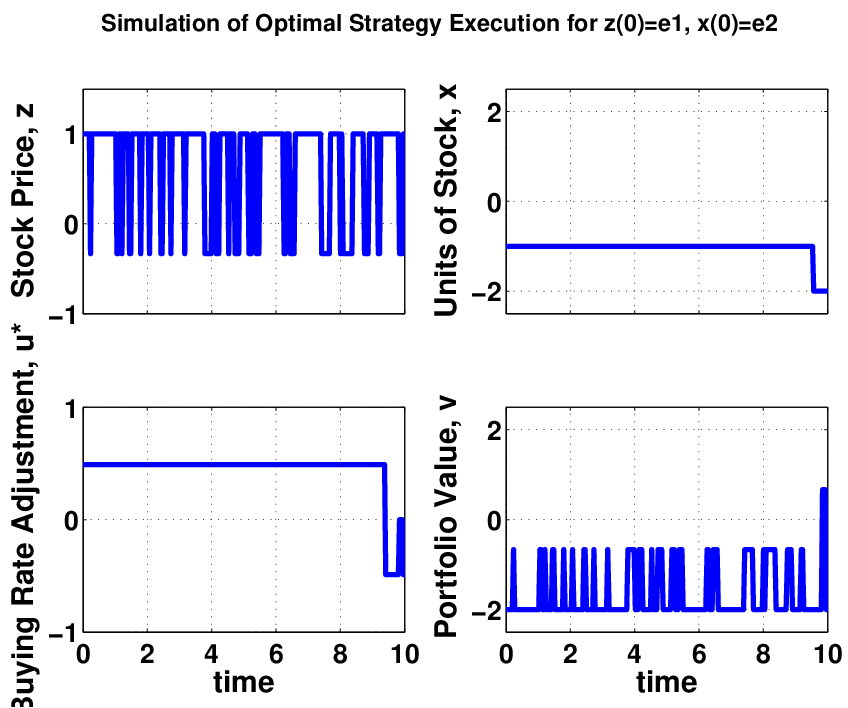
Two instances of simulation of application of the above optimal controls are shown in Figures 4 and 5. In the first case we see that one is able to benefit from $x(0)$ being in state $e_{2}$ which is the one that corresponds to maximal value of the portfolio, but in which state no trading can take place. We can hold that value and it more than offsets any devaluation due to stock price decline since the stock is more probable to have a higher price than lower. In the second simulation, we are unable to achieve state $x=e_{2}$, which happens because this state can be attained only in the less probable case of a lower stock price. However, the optimal strategy still trues to maximize the portfolio value by forcing state $x=e_{3}$ when the price is lower, but since this state is less likely, we need only switch to this sell-out strategy for a small portion of the time. The final value is most sensitive to the final trading activity. The optimal strategy allows us to maximize the portfolio value in all cases, and on the average, gives us the best value.

Our approach of using a cascade model is a more realistic model for portfolio as it is dynamic hedged. Traditional Gauss-Markov models assume continuous hedging which is unrealistic. Our model can be easily extended to include features such as transaction costs, etc. Furthermore, by modeling it as a cascade, we have a computationally scalable solution. The computation time as a function of the dimensionality of the weight s$z_{t}$ for a decomposed representation and fully coupled representation (using Bellman equations on the joint process directly) for various expiration times are shown in Figure 6. We see that the solution on a coupled state space grows exponentially with the dimensionality of $z_{t}$ whereas our solution scales linearly.

We formulate a problem that is a particular case of (4.1). Given a cascade $(z_{t},x_{t},\mathcal{U})$ with model $(A,B_{i})$ we define Problem OCP-II as the optimal control problem

$$\eta^{\ast}=\min_{u\in\mathcal{U}}\lim_{T\rightarrow\infty}\frac{1}{T}\int_{0}^{T}(p_{t}^{T}Qp_{t}+m^{T}p_{t})dt$$

(4.2)

where $Q\geq 0,$ $m$ is a vector and $p_{t}$ is the marginal probability vector of $x_{t}.$ We note that the stochastic dynamic programming principle is not directly applicable a problem of the form (4.1), and application of variational techniques at best gives us a two-point boundary value problem. Even if we did not have a cascade, the functional of the above form can result in singular arcs. To see this heuristically, consider the optimal control problem on a non-cascade defined as

	$\displaystyle\dot{p}$	$\displaystyle=$	$\displaystyle(A+\sum_{i}u_{i}B_{i})p$		(4.3)
	$\displaystyle\eta$	$\displaystyle=$	$\displaystyle\lim_{T\rightarrow\infty}\frac{1}{T}\int_{0}^{T}p^{T}Qpdt$

with $\mathcal{U=\{}a_{i}\leq u_{i}\leq b_{i}\}.$ The costate and Hamiltonian equations for this problem are

	$\displaystyle\dot{q}$	$\displaystyle=$	$\displaystyle-2Qp-A^{T}q-\left(\sum_{i}u_{i}B_{i}^{T}\right)q$
	$\displaystyle H$	$\displaystyle=$	$\displaystyle q^{T}Ap+\sum_{i}q^{T}u_{i}B_{i}p+p^{T}Qp$

so that

$${\small\frac{\partial H}{\partial u_{i}}=q^{T}B_{i}p}$$

If $q^{T}B_{i}p=0$ for any finite time interval, then we have a singular arc so that the Hamiltonian provides no useful information. Characterizing solutions to such singular optimal control problems is notoriously hard. To see how we can get a singular arc in the case above, consider a simplification of (4.3) with $A+uB$ of the form $A+uf_{i}e_{j}^{T}$ for $u\in[a,b].$For example,

$$B={\small\begin{bmatrix}0&0&0\\ 0&-1&0\\ 0&1&0\end{bmatrix}=\begin{bmatrix}0\\ -1\\ 1\end{bmatrix}\begin{bmatrix}0\\ 1\\ 0\end{bmatrix}^{T}=(-e_{2}+e_{3})e_{2}^{T}=f_{3}e_{2}^{T}~}$$

In steady state, one can show that

$$p(u)=p(0)-\frac{(e_{j}^{T}p(0))u~A^{+}f_{i}}{1+u(e_{j}^{T}A^{+}f_{i})}$$

where $A^{+}$ is the Moore-Penrose inverse of $A.$ If $\eta(u)\mathbf{~}$were of the form $c^{T}p$ (the ”usual” stochastic control case), then $u^{\ast}$ lies on the boundary of $\mathcal{U}$. In the case $\eta(u)$ is of the form $p^{T}Qp$ (i.e. the non-linear stochastic control case), then it is possible that $u^{\ast}$ is in the interior of $\mathcal{U}$.  For the class of constant controls, if $u^{\ast}\in Int(\mathcal{U)}$ then one can show by computation that the corresponding $(p(u),q(u)$ correspond to singular arcs. The above argument heuristically shows why the quadratic control problem OCP-II can be singular.

References

- [1] Brockett, R. (2008). Optimal control of observable continuous time markov chains. In Decision and Control, 2008. CDC 2008. 47th IEEE Conference on. 4269–4274.
- [2] Geerts, T. (1989). All optimal controls for the singular linear-quadratic problem without stability; a new interpretation of the optimal cost. Linear Algebra and its Applications 116, 135 – 181.
- [3] Gough, J., Belavkin, V. P., and Smolyanov, O. G. (2005). Hamiltonjacobibellman equations for quantum optimal feedback control. Journal of Optics B: Quantum and Semiclassical Optics 7, 10, S237.
- [4] Grasman, J. (1980). On a class of nearly singular optimal control problems. Stichting Mathematisch Centrum. Toegepaste Wiskunde TW 196/80 (Jan.), 1–12. http://www.narcis.nl/publication/RecordID/oai%3Acwi.nl%3A7657.
- [5] Gudder, S. (2008). Quantum Markov chains. JOURNAL OF MATHEMATICAL PHYSICS 49, 7 (JUL).
- [6] Kalenscher, T., Tobler, P. N., Huijbers, W., Daselaar, S. M., and Pennartz, C. (2010). Neural signatures of intransitive preferences. Frontiers in Human Neuroscience 4, 49.
- [7] Makowski, M. and Piotrowski, E. W. (2005). Quantum Cat’s Dilemma. eprint arXiv:quant-ph/0510110.
- [8] Noh, E.-J. and Kim, J.-H. (2011). An optimal portfolio model with stochastic volatility and stochastic interest rate. Journal of Mathematical Analysis and Applications 375, 2, 510 – 522.
- [9] Piotrowski, E. and Makowski, M. (2005). Cat’s dilemma - Transitivity vs. intransitivity. FLUCTUATION AND NOISE LETTERS 5, 1 (MAR), L85–L95.
- [10] Plateau, B. and Stewart, W. J. (1997). Stochastic automata networks. In Computational Probability. Kluwer Academic Press, 113–152.
- [11] Zhou, E., Lin, K., Fu, M., and Marcus, S. (2009). A numerical method for financial decision problems under stochastic volatility. In Winter Simulation Conference (WSC), Proceedings of the 2009. 1299 –1310.
- [12] Zilli, E. A. and Hasselmo, M. E. (2008). Analyses of markov decision process structure regarding the possible strategic use of interacting memory systems. Frontiers in Computational Neuroscience 2, 6.