Robust Bayesian model selection for heavy-tailed linear regression using finite mixtures

Define the $n$-dimensional response vector $\mathbf{Y}$, the $n\times q$ design matrix $\mathbf{X}$, the $q$-dimensional coefficient vector $\beta$ and two $K$-dimensional vectors $\mbox{\boldmath$\gamma$}=(\gamma_{1}\;\ldots\;\gamma_{K})^{\prime}$ and $\mathbf{p}=(p_{1}\;\ldots\;p_{K})^{\prime}$. Finally, let $diag(\mathbf{u}^{-1})$ be a $n$-dimensional diagonal matrix with $i$-th diagonal $u_{i}^{-1}$, $\;i=1,\ldots,n$. We propose the following general model:

where $Mult$ is the Multinomial distribution and each $F_{j}$ represents a positive distribution controlled by parameter(s) $\nu_{j}$, which may need to be truncated to guarantee that $Y_{i}$ has finite variance under each $F_{j}$.

The particular structure chosen for the variance in (2) was thought of so that, for each $j$, the variance of the model is the same - $\sigma^{2}$. This is achieved through specific choices for the functions $\gamma_{j}$ and allows us to treat $\sigma^{2}$ as a common parameter to all of the individual models. Otherwise we would need one scale parameter for each model. Therefore, in our approach, since we have a common $\mu$ and $\sigma^{2}$, the models will mainly differ from each other in terms of tail behavior which will favor the model selection procedure.

Note that each component from the mixture distribution of $u_{i}$ corresponds to one of the models being considered. Model selection is made through the posterior distribution of $\mathbf{Z}$. A subtle but important point here is the fact that there is no $i$ index for $Z_{j}$. This means that we assume that all the observations come from the same model, which poses the inference problem in the model selection framework.

Another advantage of the simultaneous approach is that it allows the use of Bayesian model averaging (Raftery et al, 1995, see). This is particularly useful in cases where more than one model have a significant posterior probability. Note that the models we consider can be quite similar in some situations - specially for higher values of the degrees of freedom (df) parameters.

The Bayesian model is fully specified by (2)-(5) and the prior distribution for the parameter vector $\mbox{\boldmath$\theta$}=(\mbox{\boldmath$\beta$},\sigma^{2},\mathbf{p},\mbox{\boldmath$\nu$})$, for $\mbox{\boldmath$\nu$}=(\nu_{1},\ldots,\nu_{K})$. Due to the complexity of the proposed model, the prior distribution plays an important role on the model identifiability and selection process and, for that reason, needs to be carefully specified.

Prior specification firstly assumes independence among all the components of $\theta$. Secondly, standard priors $\mbox{\boldmath$\beta$}\sim\mathcal{N}_{q}(\mbox{\boldmath$\mu$}_{0},\tau_{0}^{2}\mathbf{I}_{q})$ and $\sigma^{2}\sim\mathcal{I}\mathcal{G}(a_{0},b_{0})$ are adopted.

The prior distributions of the tail behavior parameters $\nu$ require special attention. This type of parameter is known to be hard to estimate (Steel and Fernandez, 1999, see) and the most promising solutions found in the literature tackle the problem through special choices of prior distributions (Fonseca et al, 2008, see). Recently, Simpson et al (2017) proposed a general family of prior distributions for flexibility parameters which includes tail behavior parameters.

In this paper we adopt the penalised complexity priors (PC priors) from Simpson et al (2017). In a simple way, the PC priors have as main principle to prefer a simpler model and penalise the more complex one. To do so, the Kullback-Leibler divergence (KLD) (Kullback and Leibler, 1951) is used to define a measure of information loss when a simpler model $h$ is used to approximate a more flexible model $f(\cdot|\nu_{j})$. The measure $d(f||h)(\nu_{j})=d(\nu_{j})=\sqrt{2KLD(f||h)}$ is defined to be a measure of complexity of model $f(\cdot|\nu_{j})$ in comparison to $h$. Further, a density function $\pi(d(\nu_{j}))=\lambda\exp(-\lambda d(\nu_{j}))$ is set for the measure $d(\nu_{j})$. Finally, the prior distribution of $\nu_{j}$ is given by

Martins and Rue (2013) showed that in a practical way, for the Student-t regression model, the PC prior can behave very similar to the Jeffrey’s priors constructed by Fonseca et al (2008). Another interesting practical usage of this prior is that the selection of an appropriate $\lambda$ is done by allowing the researcher to control the prior tail behavior of the model. For example, for the Student-t distribution the user must select $\nu^{\star}$ and $\xi$ such that $P(\nu_{j}<\nu^{\star})=\xi$, in other words, how much mass probability $\xi$ is assigned to $\nu_{j}\in(2,\nu^{\star})$ (where $j$ defines the $F_{j}$ distribution such that the response follows a Student-t distribution). Clearly, the same procedure applies for any other distribution in the NI family that has a flexibility parameter. For more details on the PC priors see Simpson et al (2017).

The prior distribution for $\mathbf{p}$ also requires special attention. Note that even in the extreme (unrealistic) case where $\mathbf{Z}$ is observed, it does not provide much information about $\mathbf{p}$, in fact, it is equivalent to the information contained in a sample of size one from a $Mult(1,p_{1},\ldots,p_{K})$ distribution. The fact that $\mathbf{Z}$ is unknown aggravates the problem. A simple and practical way to understand the consequences of this is given by the following lemma, which is a generalisation of Lemma 1 from Gonçalves et al (2013) where, to the best of our knowledge, this problem was firstly encountered.

For example, if $\alpha_{j}=1,\;\forall j$, then $\mathbb{E}[p_{j}|y]\in(1/(K+1),2/(K+1))$. This result indicates that the estimation of $\mathbf{Z}$ may be compromised by unreasonable choices of the $\alpha_{j}$’s.

A reasonable solution for this problem is to use a Dirichlet prior distribution with parameters (much) smaller than 1, which makes it sparse. It is important, though, to choose reasonable values for the $\alpha_{j}$’s, in the light of Lemma 1. Gonçalves et al (2013) claim that $\alpha_{j}=0.01,\;\forall j$ leads to good results and, in the cases where prior information is available, some of the $\alpha_{j}$’s may be increased accordingly.

We choose the following blocking scheme for the Gibbs sampler:

This blocking scheme minimises the number of blocks among the algorithms with only one MH step (which is inevitable for the df parameters). The minimum number of blocks reduces the correlation among the components, which speeds the convergence of the chain. Moreover, the most important and difficult step is the one that samples from $(\mathbf{p},\mathbf{Z},\mathbf{U})$ and sampling directly from its full conditional also favors the convergence properties of the chain.

The full conditional densities of (16) are all derived from the joint density of all random components of the model.

The first two terms on the right hand side of (3.1) are given in Section 1, for each individual model ($Z_{j}$). The remaining terms are given in Section 2.

The full conditional distributions of $\beta$ and $\sigma^{2}$ are easily devised and given by:

where $\displaystyle\mbox{\boldmath$\Sigma$}_{\beta}=\left((\tau_{0}^{2}\mathbf{I}_{q})^{-1}+(\sqrt{\mathbf{u}}\odot\mathbf{X})^{\prime}(\sqrt{\mathbf{u}}\odot\mathbf{X})/(\gamma_{j}\sigma^{2})\right)^{-1}$, $\sqrt{\mathbf{u}}$ is the $n$-dimensional vector with entries $\sqrt{\mathbf{u}_{i}}$, $\odot$ is the Hadamard product which multiplies term by term of matrices with the same dimension and $\mathbf{I}_{q}$ is the identity matrix with dimension $q$.

The df parameters are sampled in a MH step with the following transition distribution (at the $k$-th iteration):

where $f_{\mathcal{N}}(l;a,b)$ is the density of a normal distribution with mean $a$ and variance $b$ evaluated at $l$. The respective acceptance probability of a move is

where

This result is obtained by adopting the following dominating measure for both the numerator and the denominator of the acceptance probability: $\mathbb{L}^{2}\otimes\mathbb{L}\otimes m$ if $Z_{1}=0$ and $\mathbb{L}^{2}\otimes m^{2}$ if $Z_{1}=1$, where $m$ is the counting measure and $\mathbb{L}^{d}$ is the $d$-dimensional Lebesgue measure. The detailed balance along with the fact that chain is irreducible, makes this a valid MH algorithm (Tierney, 1998, see).

Note that, once we have the output of the chain, estimates of the df parameters will be based on samples of $(\nu_{t}|Z_{2}=1)$ and $(\nu_{s}|Z_{3}=1)$, which justifies the transition distributions in (18)-(20).

From (3.1), the full conditional density of $(\mathbf{p},\mathbf{Z},\mathbf{U})$ is

Defining $\displaystyle w=\sum_{j=1}^{3}r_{j}p_{j}$ and $w_{j}=r_{j}p_{j}/w$, for $j=1,2,3$, we get

We can sample from (22) using the following algorithm.

1. Simulate $\mathbf{p}$ from a density $\pi^{*}(\mathbf{p})\propto w\pi(\mathbf{p})$; 2. Simulate $\mathbf{Z}\sim Mult(1,w_{1},w_{2},w_{3})$; 3. Simulate $U_{i}$ from the density $\pi(U_{i}|\cdot),\;\forall i$; 4. OUTPUT $(\mathbf{u},\mathbf{z},\mathbf{p})$.

Steps 2 and 3 are straightforward once we have that:

where $\tilde{y}_{i}=y_{i}-\mathbf{X}_{i\cdot}\mbox{\boldmath$\beta$}$ and $\displaystyle F_{\mathcal{G}}(x;a,b)$ is the distribution function of a Gamma distribution with parameters $(a,b)$ evaluated at $x$. Moreover,

where $\mathcal{G}_{[0,1]}$ is a truncated Gamma distribution in $[0,1]$.

Step 1 is performed via rejection sampling (RS) proposing from the prior $\pi(\mathbf{p})$ and accepting with probability $\frac{w}{\max_{j}\{r_{j}\}}$. Simulated studies indicated that the algorithm is computationally efficient.

Monte Carlo estimates of the posterior distribution of $\mathbf{Z}$ (denoted by $\rho$), i.e. the models’ posterior probabilities, based on a sample of size $M$, are given by

The MCMC algorithm described in the previous section requires special attention to some aspects to guarantee its efficiency.

An indispensable strategy consists of warming up the chain inside each of the heavy-tailed models (Student-t and Slash). It contributes in several ways to the efficiency of the algorithm.

Firstly, it contributes to the mixing of the chain among the different models. If the chain starts at arbitrary values for the df parameters, it may move to high posterior density values for one of them while the other is still at a low posterior density value. This will make moves from the former model to the latter very unlike, jeopardising the convergence. More specifically, one may take the sample mean of the df parameters from their respective warm-up chains, after discarding a burn-in, as the starting values for the full chain.

Secondly, the warm-up chains will achieve or approach local convergence (inside each model). This will significantly speed the convergence of the full chain, which will have as main purpose the convergence of the $\mathbf{Z}$ coordinate.

Finally, the warm-up chains are a good opportunity to tune the MH steps of the df parameters. Given the unidimensional nature of the step and the random walk structure, the acceptance rates should be around 0,44 (Roberts et al, 1997, see).

An often common step in any regression analysis is prediction for a new configuration $\mathbf{X}_{n+1}$ of the covariates. This procedure is straightforward in a MCMC context where a sample from the posterior predictive distribution of $Y_{n+1}$ can be obtained by adding two simple steps at each iteration of the Gibbs sampler after the burn-in.

Let $\left(\mathbf{Z}^{(m)},\mbox{\boldmath$\beta$}^{(m)},{\sigma^{2}}^{(m)},\mbox{\boldmath$\gamma$}^{(m)},\nu_{t}^{(m)},\nu_{s}^{(m)}\right)$ be the state of the chain at the $m$-th iteration after the burn-in. Then, for each $m=1,2,\ldots$, firstly sample $(u_{n+1}^{(m)}|\mathbf{Z}^{(m)},\nu_{t}^{(m)},\nu_{s}^{(m)})$ from (3) and finally sample

where ${\mathbf{Z}^{\prime}}^{(m)}$ is a row vector and $\mbox{\boldmath$\gamma$}^{(m)}$ is a column vector.

One can also consider the posterior predictive distribution of $Y_{n+1}$ under one particular model, for example, the one with the highest posterior probability. In that case, it is enough to consider the sub-sample of the sample above corresponding to the chosen model.

In this study, data is generate data from one of the proposed distributions: Normal, Student-t and Slash. We consider an intercept and two covariates, i.e. $\mathbf{X}_{i\cdot}=(1,X_{i1},X_{i2})$, where $X_{i1}$ is a standard Normal random variable, $X_{i2}$ is a Bernoulli random variable with parameter $0.5$ and $i=1,\ldots,n$. The regression coefficients are $\mbox{\boldmath$\beta$}^{\top}=(1,2,-2)$. Finally for all models, the variance $\sigma^{2}$ is set to $1$. The synthetic data were generated from each of the following distributions:

1. 1.

   Normal;

2. 2.

   Student-t with degrees of freedom $\nu_{t}=15$ and $\nu_{t}=3$;

3. 3.

   Slash with degrees of freedom $\nu_{s}=3.36$ and $\nu_{s}=1.25$.

Different sample sizes $n$ are also considered - $100$, $500$, $1000$ and $5000$, giving a total of 20 scenarios. The degrees of freedom for the Slash were chosen to minimise the Kullback-Leibler divergence between the Student-t with $\nu_{t}=15$ and $\nu_{t}=3$, respectively.

For each simulated scenario a Markov chain runs for $110k$ iterations, with a burn-in of $10k$ giving a total posterior chain of $100k$ iterations. Convergence is checked using Geweke’s criterion (Geweke, 1992) since we only ran one chain. The same chain size, burn-in period and convergence verification were performed for all the examples in the paper. Notice that the parametrisation adopted allows some parameters to be estimated using the whole chain, independently of the model that is visited in each iteration. This favors the chain convergence and the MC variance of the estimates of ($\mbox{\boldmath$\beta$},\sigma^{2}$).

The summary posterior results of one run are presented in Table 1. They show that as the sample size increases the proposed methodology selects the correct model. Moreover, in the case where data is generated from the Normal distribution, not only the correct model is correctly chosen in all but one case, but also the estimated degrees of freedom of the Student-t and of the Slash distributions are high - making these distributions similar to Gaussian. Another important feature presented in the Table 1 is that the degrees of freedom parameter of the generating model is well estimated. For the non-generating model, the degrees of freedom parameter is reasonably estimated, in the sense of making the respective model as close as possible to the true one. For example, when the data is generated from the Student-t with $\nu_{t}=15$ the $\nu_{s}$ is estimated close to $3.36$, which is the value that minimises the Kullback-Leibler divergence between the two distributions. Table 1 also emphasises that, for small sample sizes $n=100$ or $n=500$, there is not enough information about the tail behavior to clearly distinguish among the models.

To check the capability of the proposed methodology in selecting the correct model, we performed a Monte Carlo study with $50$ replicates of each of the $20$ generation schemes. Table 2 presents the Mean Square Error (MSE) of the posterior estimates of the model parameters. The MSE of the $\nu$ parameters was calculated considering only the replications in which the true model was selected. The MSE of $\rho$ is the mean square error between the posterior estimate of the true model’s probability and 1. From Table 2 we can see that, even for small sample sizes, the MSE values of $\beta$ and $\sigma^{2}$ indicate a very good recovery of the true values. The MSE values of $\nu_{t}$ include some large values for small samples sizes when there is not enough information to estimate precisely the degrees of freedom. The difference in the magnitudes of $\nu_{t}$ and $\nu_{s}$ are explained by the difference in the scale of those parameters. Finally, the last column of the table shows the percentage of times that the correct model was selected (i.e. had the highest posterior probability).

This study investigates how the model selection procedure and the parameter estimation is affected in the presence of correlated covariates. We generate data from a model with $e_{i}\sim\mathcal{T}(0,1,3)$, $\beta=(1,2,-2,1)$, $\mathbf{X}_{i}=(1,X_{i1},X_{i2},X_{i3})$ and $X_{i3}=2X_{2i}+\mathcal{N}(0,0.5)$ which induces an average correlation of $0.9$ between the two covariates.

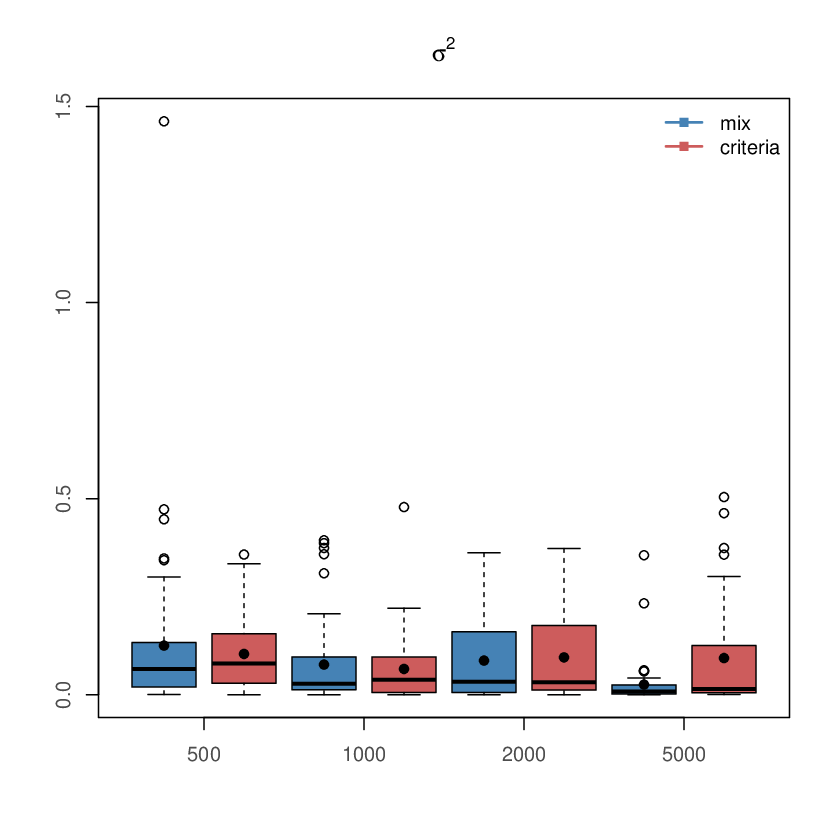
We reproduce $50$ replicates of this scenario with different sample sizes $n=500$, $1000$, $2000$ and $5000$. Table 3 shows the percentage of times that the proposed methodology selects each model and compares it with the other model selection criteria. It is clear that the traditional criteria have problems to distinguish between models with heavy tails even when the sample size increases, whilst the proposed methodology performs a robust selection specially for large sample sizes where tail information is more abundant.

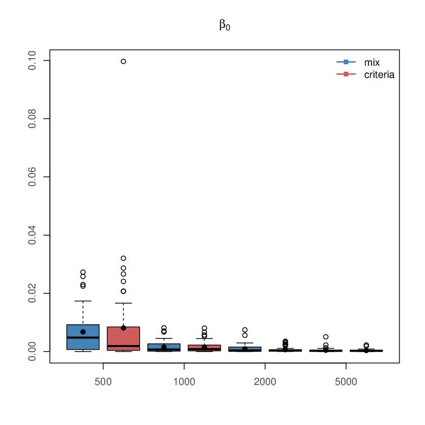
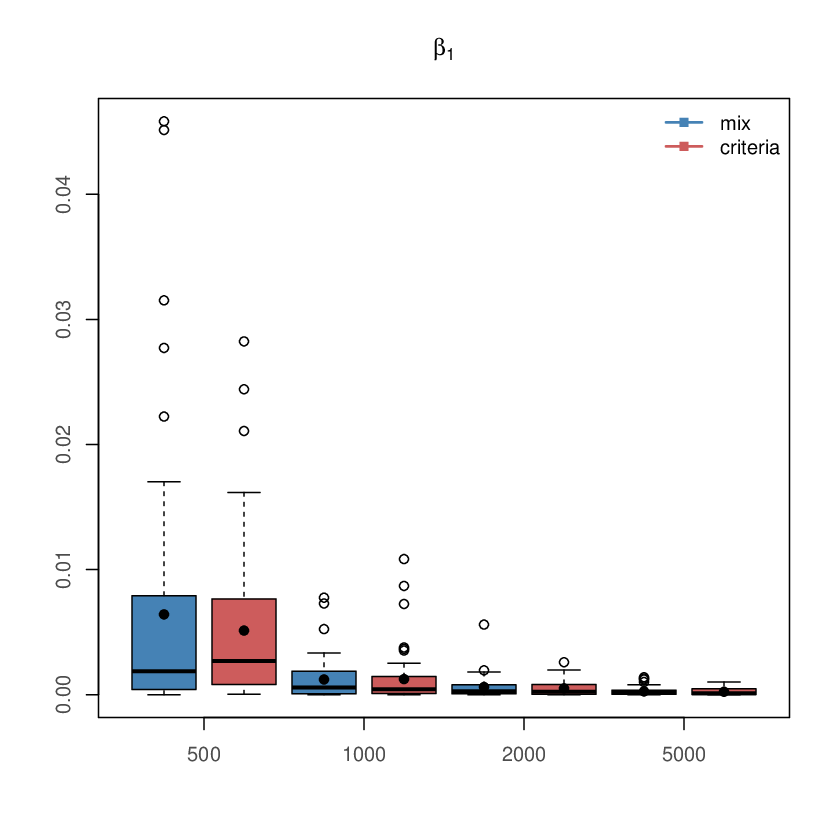
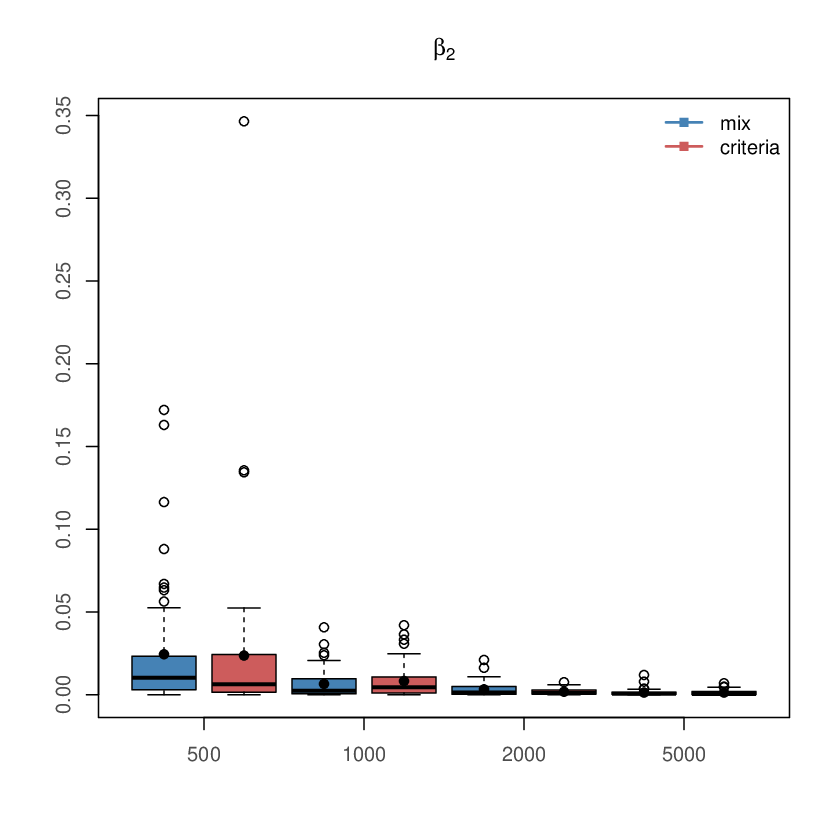
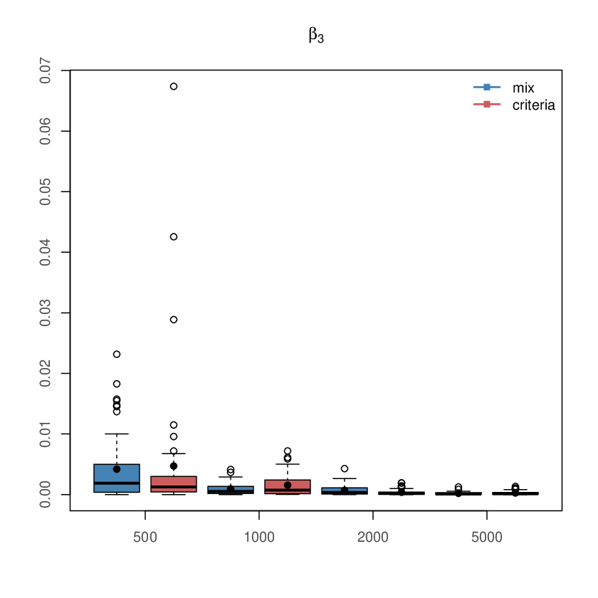
Figure 1 shows some results regarding the estimation of the regression coefficients. They are quite similar between the proposed methodology and the other model selection criteria. The same, however, does not happen when we look at the estimates for the variance $\sigma^{2}$. The poor performance of the other criteria in selecting the correct model is clearly reflected in the estimation of the variance, which is significantly overcome by the respective estimates obtained with the proposed methodology.

In this study the generating distribution for the error term is not a specific distribution as in Section 4.1 and 4.2, but a mixture of the Normal, Student-t and Slash distributions. More specifically, we consider $e_{i}\sim 0.1\mathcal{N}(0,1)+0.6\mathcal{T}(0,1,4.00)+0.3\mathcal{S}(0,1,1.15)$, with the same $\mathbf{X}$, $\beta$’s and $\sigma^{2}$ from Study I. The sample sizes $n$ considered are the same as in Study II.

Again, $50$ replications are generated. It is important to notice that our modeling framework to perform robust model selection cannot retrieve the generating model, since we assume that all the residuals must be from the same distribution. Nevertheless, a good fit may still be provided by one of the individual models. Table 4 show the result of one of the $50$ replications. It is clear that the posterior distribution identifies the Student-t distribution as the best candidate model, specially as the sample size increases.

For sample size $2000$, Figure 3 shows the fit of the selected model (Student-t) and the other two models, Normal and Slash, fitted individually. It also shows the true generating distribution for the error term. It is clear that, although the posterior distribution is different from the true generating distribution, by definition, it approximates fairly very well the original one.

Table 5 shows that the proposed model consistently chooses the dominating model (student-t) as the sample size increases. The same does not happen for the other model selection criteria.

In this section we introduce a biomedical study from the Australian Institute of Sports (AIS) in $202$ athletes (Cook and Weisberg, 1994). To exemplify our modeling we consider the body mass index (BMI) as our response and the percentage of body fat (Bfat) as our covariate. This way, we have a regression model with $\mathbf{X}_{i\cdot}=(1,\mbox{Bfat}_{i})$ for $i=1,\ldots,202$.

We fit each individual model separately and the proposed mixture model. Results are presented in Tables 6 and 7. Note that, although the Slash model is chosen by all the criteria, and the estimates of the regression coefficients are similar between the individual fit and our model, significant, though not large, differences can be found for the estimates of the variance $\sigma^{2}$. This highlights the model averaging feature of our approach, which is particularly appealing when one of the models is not chosen with very high probability - in this example $\rho$ - $(0.001,0.304,0.695)$.

The wage rate data set presented in Mroz (1987) is used to extend our modeling framework for censored data. The data consist of the wage of 753 married white women, with ages between 30 and 60 years old in 1975. Out of the 753 women considered in this study, 428 worked at some point during that year. When the wives did not work in 1975, the wage rates were set equal to zero. However, it is considered that they may had a cost in that year and, therefore, these observations are considered left censored at zero. The considered response is $Y_{i}$ - the wage rate, and the explanatory variables are the wife’s age ($X_{1i}$), years of schooling ($X_{2i}$), number of children younger than six years old in the household ($X_{3i}$) and number of children between six and nineteen years old ($X_{4i}$). Thus, $\mathbf{X}_{i\cdot}=(1,X_{1i},X_{2i},X_{3i},X_{4i})$, $i=1,\ldots,753$.

Since the Wage data is censored, we have the following characteristic for our response variables

with $\kappa_{i}=0$.

Suppose that, out of the $n$ responses, $C$ of them are censored as $\kappa_{i}$. From a Bayesian perspective, these observations, $\mathbf{Y}_{C}=(y_{1},\ldots,y_{C})$, can be viewed as latent and sampled at each step of the MCMC. Because of the model structure presented in (6)-(3), it is simple to notice that

where $\mathcal{TN}$ is a truncated Normal distribution with limits $\lfloor-\infty,\kappa_{c}\rfloor$. Therefore, we simply add a new sampling step in the blocking scheme as

This simple extension allows our modeling framework to deal with any kind of censored data, where, for each type of censoring scheme, the new limits of (27) must be calculated.

To obtain our final chain with $100k$ observations, a Markov Chain of $110k$ iterations is run and the first $10k$ observations are discarded for burn-in. The posterior estimate for $\rho$ is $(0.000,0.025,0.975)$, which indicates the Slash distribution as the preferred one.

Table 8 summarises the posterior results. Garay et al (2015) studied this data set from a Bayesian perspective fitting a variety of independent models in the NI family. In their study, the Slash distribution was selected as the preferred one as in our case. Moreover, the posterior mean estimates of the fixed effects parameters in Table 8 are very similar to the ones presented in Garay et al (2015) as well as the statistical significance of each covariate. The wife’s age, the number of children younger than six years old in the household and the number of children between six and nineteen years old tend to decrease the wage rate, while years of schooling tend to increase the salary. The posterior estimates encountered by Garay et al (2015) for $\nu_{s}$ and $\nu_{t}$, fitting separate models, were $1.438$ and $5.279$, respectively, which agree with our results. Our mixture model approach was able to correctly capture the Slash distribution without separately fitting the three models. Moreover, it provides a high computational gain given the high posterior probability of the Slash model.

References

- Andrews and Mallows (1974) Andrews DF, Mallows SL (1974) Scale mixtures of normal distributions. Journal of the Royal Statistical Society, Series B 36:99–102
- Basso et al (2010) Basso RM, Lachos VH, Cabral CRB, Ghosh P (2010) Robust mixture modeling based on scale mixtures of skew-normal distributions. Computational Statistics & Data Analysis 54(12):2926–2941
- Cabral et al (2012) Cabral CRB, Lachos VH, Prates MO (2012) Multivariate mixture modeling using skew-normal independent distributions. Computational Statistics & Data Analysis 56(1):126–142
- Carlin (2006) Carlin BP (2006) Comments to discussion of deviance information criteria for missing data. Bayesian Analysis 1(4):675–676
- Chen (2006) Chen MH (2006) Comments to discussion of deviance information criteria for missing data. Bayesian Analysis 1(4):677–680
- Choy and Chan (2008) Choy STB, Chan JSK (2008) Scale mixtures distributions in statistical modelling. Australian & New Zeland Journal of Statistics 50:135–146
- Cook and Weisberg (1994) Cook RD, Weisberg S (1994) An Introduction to Regression Graphics. Wiley, New York
- Dey et al (1997) Dey DK, Chen MH, Chang H (1997) Bayesian approach for nonlinear random effects models. Biometrics 53:1239–1252
- Fernandez and Steel (1999) Fernandez C, Steel MFJ (1999) Multivariate student-t regression models: Pitfalls and inference. Biometrika 86(1):153–167
- Fonseca et al (2008) Fonseca TCO, Ferreira MAR, Migon HS (2008) Objective bayesian analysis for the student-t regression model. Biometrika 95:325–333
- Galea et al (2003) Galea M, Paula GA, Uribe-Opazo M (2003) On influence diagnostic in univariate elliptical linear regression models. Statistical Papers 44(1):23–45
- Galea et al (2005) Galea M, Paula GA, Cysneiros FJA (2005) On diagnostics in symmetrical nonlinear models. Statistics & Probability Letters 73:459–467
- Garay et al (2015) Garay AM, Bolfarine H, Lachos VH, Cabral CRB (2015) Bayesian analysis of censored linear regression models with scale mixtures of normal distributions. Journal of Applied Statistics 42(12):2694–2714
- Geisser and Eddy (1979) Geisser S, Eddy WF (1979) A predictive approach to model selection (Corr: V75 p765). Journal of the American Statistical Association 74:153–160
- Gelman et al (2014) Gelman A, Hwang J, Vehtari A (2014) Understanding predictive information criteria for Bayesian models. Statistics and Computing 24:997–1016
- George and McCulloch (1993) George EI, McCulloch RE (1993) Variable selection via Gibbs sampling. Journal of American Statistical Association 85:398–409
- Geweke (1992) Geweke J (1992) Evaluating the accuracy of sampling-based approaches to the calculation of posterior moments (Disc: P189-193). In: Bernardo JM, Berger JO, Dawid AP, Smith AFM (eds) Bayesian Statistics 4. Proceedings of the Fourth Valencia International Meeting, Clarendon Press [Oxford University Press], pp 169–188
- Gonçalves et al (2013) Gonçalves FB, Gamerman D, Soares TM (2013) Simultaneous multifactor DIF analysis and detection in item response theory. Computational Statistics and Data Analysis 59:144–160
- Kullback and Leibler (1951) Kullback S, Leibler RA (1951) On information and sufficiency. The Annals of Mathematical Statistics pp 79–86
- Lachos et al (2010) Lachos VH, Ghosh P, Arellano-Valle R (2010) Likelihood based inference for skew-normal independent linear mixed models. Statistica Sinica 20:303–322
- Lachos et al (2011) Lachos VH, Angolini T, Abanto-Valle C (2011) On estimation and local influence analysis for measurement errors models under heavy-tailed distributions. Statistical Papers 52(3):567–590
- Lange and Sinsheimer (1993) Lange KL, Sinsheimer JS (1993) Normal/independent distributions and their applications in robust regression. J Comput Graph Stat 2:175–198
- Lange et al (1989) Lange KL, Little R, Taylor J (1989) Robust statistical modeling using t distribution. Journal of the American Statistical Association 84:881–896
- Lin and Cao (2013) Lin JG, Cao CZ (2013) On estimation of measurement error models with replication under heavy-tailed distributions. Computational Statistics 28(2):809–829
- Martins and Rue (2013) Martins TG, Rue H (2013) Prior for flexibility parameters: the student’s t case. Preprint 08/2013, Norwegian University of Science and Technology
- Mroz (1987) Mroz TA (1987) The sensitivity of an empirical model of married women´s hours of work to economic and statistical assumptions. Econometrica 55:765–799
- Osorio et al (2007) Osorio F, Paula GA, Galea M (2007) Assessment of local influence in elliptical linear models with longitudinal structure. Computational Statistics & Data Analysis 51(9):4354–4368
- Pinheiro et al (2001) Pinheiro JC, Liu C, Wu YN (2001) Efficient algorithms for robust estimation in linear mixed-effects models using the multivariate t distribution. Journal of Computational and Graphical Statistics 10(2):249–276
- Raftery et al (1995) Raftery A, Madigan D, Volinsky CT (1995) Accounting for model uncertainty in survival analysis improves predictive performance. In: In Bayesian Statistics 5, University Press, pp 323–349
- Roberts et al (1997) Roberts GO, Gelman A, Gilks WR (1997) Weak convergence and optimal scaling of random walk metropolis algorithms. Annals of Applied Probability 7:110–120
- Rosa et al (2003) Rosa G, Padovani C, Gianola D (2003) Robust linear mixed models with normal/independent distributions and bayesian mcmc implementation. Biometrical Journal 45(5):573–590
- Simpson et al (2017) Simpson D, Rue H, Riebler A, Martins TG, Sørbye SH (2017) Penalising model component complexity: A principled, practical approach to constructing priors. Statistical Science 32:1–28
- Spiegelhalter et al (2002) Spiegelhalter D, Best N, Carlin B, Van Der Linde A (2002) Bayesian measures of model complexity and fit. Journal of the Royal Statistical Society, Series B 64:583–639
- Steel and Fernandez (1999) Steel MFJ, Fernandez C (1999) Multivariate Student-t regression models: pitfalls and inference. Biometrika 86:153–168
- Tierney (1998) Tierney L (1998) A note on Metropolis-Hastings kernels for general state spaces. The Annals of Applied Probability 8:1–9
- Watanabe (2010) Watanabe S (2010) Asymptotic equivalence of bayes cross validation and widely applicable information criterion in singular learning theory. Journal of Machine Learning Research 11:3571–3594