The Geodesic Light-Cone Coordinates,
an Adapted System for Light-Signal-Based Cosmology

The more observational precision increases, the more inhomogeneous our Universe looks. Supernovæ [1], lensing [2, 3, 4], and other light-propagated observables will soon encounter associated complications [5, 6, 7, 8, 9, 10, 11, 12, 13]. We present coordinates first developed to simplify averages of scalars on our past light-cone [14], next used to estimate the effect of inhomogeneities on luminosity distance [15, 16, 17, 18], Hubble diagram [19, 20], and recently applied to lensing quantities [21] (and illustrated in a Lemaître-Tolman-Bondi model), following this historical order.

We define a light-cone adapted metric (close to “observational coordinates”[22, 23], but different [24]) composed of 6 arbitrary functions ($\Upsilon$, $U^{a}$, $\gamma_{ab}$) and totally gauged fixed :

This metric uses a null coordinate $w$ defining past light cones, the proper time of a geodesic observer $\tau$, and angles $\tilde{\theta}^{a}$ that photons keep along their path orthogonal to a 2-spheres $\Sigma(w,\tau)$ of constant time in our past light-cone (see Fig. 1). In the FLRW limit : $w=\eta+r$ (conformal time, radius), $\tau=t$ (cosmic time), $(\tilde{\theta}^{1},\tilde{\theta}^{2})=(\theta,\phi)$, $\Upsilon=a(t)$, $U^{a}=0$, $\gamma_{ab}=a^{2}r^{2}(1,\sin^{2}\theta)$. In general [24] $\Upsilon$ is like an inhomogeneous scale factor (lapse function), $U^{a}$ like a shift-vector and $\gamma_{ab}$ is the metric inside $\Sigma(w,\tau)$. We can notice two direct simplifications in GLC which, combined together, give the distance-redshift relation :

These coordinates share similarities with historical ones such as “observational coordinates" [25, 26, 22, 23], (see elements of comparison in Ref.[24]) or the “optical coordinates" [27].

The light-cone average[14] of a scalar $S$ (e.g. $d_{L}~,~d_{L}^{-2}$) is in general given by $\left\langle S\right\rangle(V_{0},A_{0})=I(S;V_{0},A_{0})/I(1;V_{0},A_{0})$ and we define the average integral to be gauge invariant, invariant under $(A,V)\rightarrow(\tilde{A}(A),\tilde{V}(V))$ and general coordinate transformations :

where ${\mathcal{N}}(V,A,\partial_{\mu})$ is a normalization, $D(X)=\delta_{D}(X)$ or $\Theta(X)$ (Heaviside function) :

Among these 3 types of averages, $\left\langle S\right\rangle_{V_{0},A_{0}}$ is closer to physical observables as it averages over the deformed 2-sphere embedded in the light-cone $V=V_{0}$ and a spatial hypersurface $A=A_{0}$. In GLC coordinates (where $V\rightarrow w$, $A\rightarrow\tau$) we can simplify the average and use Eq. (2) to get (with $\tau_{z}\equiv\tau(z_{s},w_{o},\widetilde{\theta}^{a}))$ :

allowing us to average scalars on the sky, at a certain redshift.

The GLC metric enables the computation of $d_{L}(z)$ at $\mathcal{O}(2)$ in the Newtonian gauge (NG) :

with $\Phi=\psi+\frac{1}{2}\phi^{(2)}$ , $\Psi=\psi+\frac{1}{2}\psi^{(2)}$ the gauge invariant Bardeen potentials (no matter shear at $\mathcal{O}(1)$, or see Ref.[17]). Establishing the full transformation between GLC and NG coordinates at $\mathcal{O}(2)$ in (scalar) perturbations, we get $(\tau,w,\widetilde{\theta}^{1},\widetilde{\theta}^{2})={\rm func}(\eta,r,\theta,\phi)$ and $(\Upsilon,U^{a},\gamma^{ab})={\rm func}(\psi,\psi^{(2)},\phi^{(2)})$ which allows us to compute $d_{L}$ to $\mathcal{O}(2)$ (using Eq. (3)) :

The first order in scalar perturbations is given by :

with $\mathcal{H}_{s}=a^{\prime}(\eta_{s})/a(\eta_{s})$, $\Delta\eta=\eta_{o}-\eta_{s}^{(0)}$, containing (Integrated) Sachs-Wolfe ([I]SW), Doppler, and lensing (convergence) effects  :

where ‘$o$’ (‘$s$’) denote quantities evaluated at the observer (source), and we defined :

Similarly obtained $\mathcal{O}(2)$ corrections contain (see Refs.[16, 24]) :

• •

  Two dominant terms : $(\mbox{Doppler})^{2}$, $(\mbox{Lensing})^{2}$,
  

• •

  Combinations of $\mathcal{O}(1)$-terms : $\psi_{s}^{2}$, $(\mbox{[I]SW})^{2}$, $\mbox{[I]SW}\times\mbox{Doppler}$, $(\psi_{s},Q_{s})\times$ (Lensing, [I]SW, Doppler),
  

• •

  Genuine $\mathcal{O}(2)$-terms : $\psi_{s}^{(2)}$, $Q_{s}^{(2)}$, $\mbox{Lensing}^{(2)}\!=\!\frac{1}{2}\nabla_{a}\tilde{\theta}^{a(2)}$,
  

• •

  New integrated effects : $\frac{1}{4\Delta\eta}\int_{\eta_{s}^{(0)+}}^{\eta_{s}^{(0)-}}\mathrm{d}x~\left[4\hat{\psi}~\partial_{+}Q+\hat{\gamma}_{0}^{ab}~\partial_{a}Q~\partial_{b}Q\right](\eta_{s}^{(0)+},x,\theta^{a})$,
  

• •

  Angle deformations : $(\gamma_{0})_{ab}\partial_{+}\tilde{\theta}^{a(1)}\partial_{-}\tilde{\theta}^{b(1)}~~,~~\partial_{a}\tilde{\theta}^{b(1)}\partial_{b}\tilde{\theta}^{a(1)}$  ,
  

• •

  Redshift perturbations from Eq. (2), involving transverse peculiar velocities :
  $\gamma_{0}^{ab}\left(\partial_{a}P~\partial_{b}P~,~\partial_{a}Q~\partial_{b}Q~,~\partial_{a}Q~\partial_{b}P\right)$ , $\partial_{+}\int_{\eta_{+}}^{\eta_{-}}\mathrm{d}x\left[4\hat{\psi}~\partial_{+}Q+\hat{\gamma}_{0}^{ab}\partial_{a}Q~\partial_{b}Q\right]$ , $\int_{\eta_{in}}^{\eta}\mathrm{d}\eta^{\prime}~\frac{a(\eta^{\prime})}{a(\eta)}\partial_{r}\left[\left(\partial_{r}P\right)^{2}+\gamma_{0}^{ab}\partial_{a}P~\partial_{b}P\right]$ ,
  

• •

  Other important terms : Lens-Lens coupling, corrections to Born approximation.

These $\mathcal{O}(2)$ results were confirmed recently[28] working directly in terms of GLC coordinates rather than NG. An independent derivation [29, 30] lead to similar results, but a rigorous comparison with Ref.[16] is still lacking. Results were also given for vector/tensor perturbations[16] (Poisson gauge) and extended to the case with $\mathcal{O}(1)$ anisotropic stress [17, 18].

In Sec. 4 we expressed $d_{L}$ in terms of $(\psi,\psi^{(2)},\phi^{(2)})$, hence it needs a description of the Bardeen potentials at $\mathcal{O}(1,2)$. We decompose the first order gravitational potential $\psi$ in Fourier modes and denote by $\overline{(...)}$ the ensemble (or stochastic) average over perturbations. The $\mathcal{O}(2)$ potentials can be related to $\psi$ by[31] : $\psi^{(2)},\phi^{(2)}\propto\nabla^{-2}(\partial_{i}\psi\partial^{i}\psi)~,~\partial_{i}\psi\partial^{i}\psi$. Hence we can combine light-cone and stochastic averages in order to study the effect of statistical perturbations on the whole sky. For example, the (trivial) average of $\psi^{2}$ gives : $\overline{\left\langle\psi_{s}^{2}\right\rangle}=\int_{0}^{\infty}\frac{\mathrm{d}k}{k}\mathcal{P}_{\psi}(k)$ where $\mathcal{P}_{\psi}(k)\equiv(k^{3}/2\pi^{2})|\psi_{k}(\eta)|^{2}=(3/5)^{2}A(k/k_{0})^{n_{s}-1}T^{2}(k)\,g^{2}(z)$ is the power spectrum describing perturbations. At linear order, with $A$, $n_{s}$, $k_{0}$ taken from WMAP, $T(k)$ is a transfer function[32] including a baryonic component (Silk damping), and $g(z)$ is the growth factor describing the recent time evolution of perturbations. In CDM we get exactly the spectral coefficients coming from each correction of $d_{L}(z_{s},\theta^{a})$ described in Sec. 4 : $\overline{\left\langle d_{L}\right\rangle}=\int_{0}^{\infty}\frac{\mathrm{d}k}{k}\mathcal{P}_{\psi}(k)\,C(k\Delta\eta)$. We do the same in $\Lambda$CDM, with reasonable assumptions to simplify integrations [20], and also with a non-linear power spectrum [33, 34].

Like $d_{L}$ one can also average the flux $\Phi=L/(4\pi d_{L}^{2})\simeq\Phi_{0}+\Phi_{1}+\Phi_{2}$. We get :

• •

  $\overline{\langle d_{L}^{-2}\rangle}\equiv(d_{L}^{FLRW})^{-2}\left[1+f_{\Phi}(z)\right]$ where $f_{\Phi}(z)\simeq f(z)\int_{0}^{\infty}\frac{\mathrm{d}k}{k}\left(\frac{k}{{\cal H}_{0}}\right)^{2}\mathcal{P}_{\psi}(k)$   ,
  

• •

  $\overline{\langle d_{L}\rangle}(z)=d_{L}^{FLRW}\left[1+f_{d}(z)\right]$ with $f_{d}=-(1/2)f_{\Phi}+(3/8)\overline{\langle\left(\Phi_{1}/\Phi_{0}\right)^{2}\rangle}$  .

Corrections to $d_{L}$ involve a flux variance dominated by peculiar velocity and lensing :

as shown in Fig. 2 for realistic (non-)linear power spectra [20]. It turns out that the luminosity flux is minimally affected by lensing w.r.t. other scalar observables at large redshift. This calculation can be seen as a check at $\mathcal{O}(2)$ of Weinberg’s argument of flux conservation [35] and has also been confirmed by recent papers through different approaches [36, 37, 38].

Similarly, we can get the average/dispersion of the distance modulus :

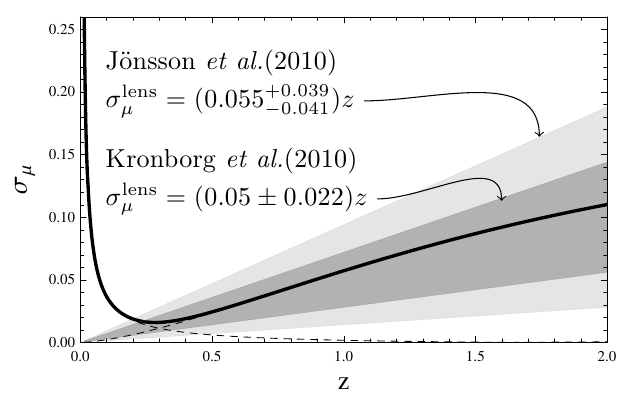
Compared to the Union 2 data and using a non-linear power spectrum in $\Lambda$CDM (Fig. 3, Left), we find that peculiar velocities explain well the scatter at small $z$ and that lensing explains only part of the scatter at large $z$. Finally, we can compare our dispersion on the Hubble diagram with the experimental estimations coming from lensing[39, 40] (Fig. 3, Right). We find that the total effect is well fitted by Doppler ($z\leq 0.2$) + lensing ($z>0.3$) effects and that the lensing prediction is in great agreement with experiments so far.

We now consider lensing[21], motivated by Sec. 5 and recent work[41] on galaxy number counts in GLC. The relative separation of two neighbour light rays simultaneously emitted from a source $S$ and converging to an observer $O$ follows the geodesic deviation eq. (GDE) : $\nabla_{\lambda}^{2}\xi^{\mu}=R^{\mu}_{~\,\alpha\beta\nu}k^{\alpha}k^{\nu}\xi^{\beta}$ with $\nabla_{\lambda}\equiv{\rm D}/\mathrm{d}\lambda\equiv k^{\mu}\nabla_{\mu}$, $k^{\mu}$ the photon momentum, $\lambda$ an affine parameter along the photon path, and $\xi^{\mu}$ an orthogonal displacement w.r.t. to the rays. We project the GDE on the Sachs basis $\{s^{\mu}_{A}\}_{A=1,2}$ (two zweibeins with flat index $A=1,2$) : $g_{\mu\nu}s^{\mu}_{A}s^{\nu}_{B}=\delta_{AB}~,~s^{\mu}_{A}u_{\mu}=0~,~s^{\mu}_{A}k_{\mu}=0~,~\Pi^{\mu}_{\nu}\nabla_{\lambda}s^{\nu}_{A}=0$ ; with $u_{\mu}$ the peculiar velocity of comoving fluid ($S$, $O$ comoving too), $\Pi^{\mu}_{\nu}$ a “screen" projector orthogonal to $u_{\mu}$ and $u_{\mu}+\left(u^{\alpha}k_{\alpha}\right)^{-1}k_{\mu}$. We define the Jacobi map $J^{A}_{B}$, from the observed sky angle $\bar{\theta}_{o}^{A}$ to $\xi^{A}\equiv\xi^{\mu}s^{A}_{\mu}$, by $\xi^{A}(\lambda)=J^{A}_{B}(\lambda,\lambda_{o})\,\bar{\theta}_{o}^{A}$. Projected quantities $\xi^{A}$ and $R^{A}_{B}\equiv R_{\alpha\beta\nu\mu}k^{\alpha}k^{\nu}s^{\beta}_{B}s^{\mu}_{A}$ (optical tidal matrix) bring us the Jacobi equation (see e.g. Refs.[6, 42]) :

A direct resolution of Eq. (12) gives the angular distance of the source $d_{A}(\lambda_{s})\equiv\sqrt{dS_{s}/d^{2}\Omega_{o}}=\sqrt{\det J^{A}_{B}(\lambda_{s},\lambda_{o})}$. Also, the (unlensed) angular position of the source $\bar{\theta}^{A}_{s}$ and the observed lensed position $\bar{\theta}^{A}_{o}$ (of the image) are given by : $\bar{\theta}^{A}_{s}=\left(\xi^{A}/\bar{d}_{A}\right)_{s}$, $\bar{\theta}^{A}_{o}=\left(k^{\mu}\partial_{\mu}\xi^{A}/k^{\mu}u_{\mu}\right)_{o}$, where $\bar{d}_{A}$ is the homogeneous and isotropic background our model refers to. This allows us to define the so-called amplification matrix as :

which defines the lensing quantities : $\kappa=1-\text{tr}J^{A}_{B}/2\bar{d}_{A}$ (convergence), $\hat{\omega}=|J^{1}_{2}-J^{2}_{1}|/2\bar{d}_{A}$ (vorticity), $|\hat{\gamma}|\equiv\sqrt{(\hat{\gamma}_{1})^{2}+(\hat{\gamma}_{2})^{2}}=\sqrt{(1-\kappa)^{2}+\hat{\omega}^{2}-\mu^{-1}}$ (shear) and $\mu\equiv 1/(\det\mathcal{A})=\bar{d}_{A}^{2}/\det J^{A}_{B}$ (magnification).

Let us now turn to the GLC coordinates and express these lensing quantities in it. First, the zweibeins are written as $s^{\mu}_{A}=(s^{\tau}_{A},0,s^{a}_{A})$ and $k^{\mu}\equiv\omega\Upsilon^{-1}\delta^{\mu}_{\tau}$ (with $\omega$ a pure constant). Second, the solution to Eqs. (12) and (13) is :

where $(\ldots)^{\mbox{\Large$\cdot$}}\equiv\partial_{\tau}(\ldots)$ . The angular distance and the magnification become :

involving $\bar{d}_{A}=a^{2}(\tau)r^{2}$ with $r=w-\int\mathrm{d}\tau/a(\tau)$ measured from the observer and $\Phi$ ($\bar{\Phi}$) the flux in the in(homogeneous) geometry. Expressions for the zweibeins can be obtained in the GLC coordinates[21], but it is more convenient to compute the squared lensing quantities, combined with $s^{A}_{a}s^{A}_{b}=\gamma_{ab}$ and $\epsilon_{AB}\,s^{A}_{a}s^{B}_{b}=\sqrt{\gamma}\,\epsilon_{ab}$ ($\epsilon$ the anti-sym. symbol), to get :

We thus have general lensing quantities expressed with only 3 metric functions (of $\gamma_{ab}$), showing the great advantage of working in GLC coordinates.

The Jacobi Eq. (12) can be rewritten as a first order differential equation for the so-called deformation matrix :

involving the optical scalars, $\hat{\theta}$ (expansion scalar) and $\hat{\sigma}\equiv\hat{\sigma}_{1}+i\hat{\sigma}_{2}$ (shear scalar), and known as the Sachs equations :

The RHS terms are the Ricci and Weyl focusing and are defined as follows :

where $R_{\alpha\beta}$ is the Ricci tensor, $C_{\alpha\beta\mu\nu}$ the Weyl tensor, and $\Sigma^{\mu}\equiv s^{\mu}_{1}+is^{\mu}_{2}$. As well as the amplification matrix, the deformation matrix simplifies in the GLC coordinates as :

Using $s^{a}_{A}s^{b}_{A}=\gamma^{ab}$ we get the optical scalars :

We also get the Ricci and Weyl focusing in GLC coordinates :

where $Y_{ab}\equiv\ddot{\gamma}_{ab}-(\dot{\Upsilon}/\Upsilon)\dot{\gamma}_{ab}-(1/2)\dot{\gamma}_{ac}\gamma^{cd}\dot{\gamma}_{db}$ depends only on $\gamma_{ab}$, $\Upsilon$ and their time derivatives. This proves again the usefulness of GLC coordinates for lensing and it was illustrated[21] by the computation of lensing quantities in the case of an off-center observer in a Lemaître-Tolman-Bondi model (considering only the decaying mode).

We have shown that there are many advantages in using the GLC coordinates. They are indeed adapted to calculations involving light-propagation, they can also be used for weak lensing (where $\gamma_{ab}$ acts as a screen), and may help to get new predictions on cosmology or to study other aspects of lensing (e.g. lensing statistics).

I want to thank the Fourteenth Marcel Grossmann Meeting for giving me the opportunity to share these properties of GLC coordinates in two parallel sessions and for giving me the occasion to write this document. My researches are supported by the project GLENCO lead by B. Metcalf, funded under the FP7, Ideas, Grant Agreement n. 259349.

References

- [1] A. Conley, J. Guy, M. Sullivan, N. Regnault, P. Astier, et al., “Supernova Constraints and Systematic Uncertainties from the First 3 Years of the Supernova Legacy Survey,” Astrophys. J. Suppl. 192 (2011) 1, arXiv:1104.1443 [astro-ph.CO].
- [2] P. Schneider, G. Meylan, C. Kochanek, P. Jetzer, P. North, and J. Wambsganss, Gravitational Lensing: Strong, Weak and Micro: Saas-Fee Advanced Course 33. Saas-Fee Advanced Course. Springer Berlin Heidelberg, 2006. https://books.google.it/books?id=AF8-ErlCb94C.
- [3] Euclid Theory Working Group Collaboration, L. Amendola et al., “Cosmology and fundamental physics with the Euclid satellite,” Living Rev.Rel. 16 (2013) 6, arXiv:1206.1225 [astro-ph.CO].
- [4] LSST Science Collaboration, P. A. Abell, J. Allison, S. F. Anderson, J. R. Andrew, J. R. P. Angel, L. Armus, D. Arnett, S. J. Asztalos, T. S. Axelrod, and et al., “LSST Science Book, Version 2.0,” ArXiv e-prints (Dec., 2009) , arXiv:0912.0201 [astro-ph.IM].
- [5] C. Clarkson, G. F. Ellis, A. Faltenbacher, R. Maartens, O. Umeh, et al., “(Mis-)Interpreting supernovae observations in a lumpy universe,” Mon.Not.Roy.Astron.Soc. 426 (2012) 1121–1136, arXiv:1109.2484 [astro-ph.CO].
- [6] P. Fleury, H. Dupuy, and J.-P. Uzan, “Interpretation of the Hubble diagram in a nonhomogeneous universe,” Physical Review D 87, 123526 (2013) , arXiv:1302.5308 [astro-ph.CO].
- [7] M. Lavinto and S. Rasanen, “CMB seen through random Swiss Cheese,” arXiv:1507.06590 [astro-ph.CO].
- [8] G. Ellis, “Republication of: Relativistic cosmology,” General Relativity and Gravitation 41 (2009) 581–660. http://dx.doi.org/10.1007/s10714-009-0760-7.
- [9] T. Buchert and S. Rasanen, “Backreaction in late-time cosmology,” Ann. Rev. Nucl. Part. Sci. 62 (2012) 57–79, arXiv:1112.5335 [astro-ph.CO].
- [10] T. Buchert, “Toward physical cosmology: focus on inhomogeneous geometry and its non-perturbative effects,” Class. Quant. Grav. 28 (2011) 164007, arXiv:1103.2016 [gr-qc].
- [11] C. Clarkson, G. Ellis, J. Larena, and O. Umeh, “Does the growth of structure affect our dynamical models of the universe? The averaging, backreaction and fitting problems in cosmology,” Rept. Prog. Phys. 74 (2011) 112901, arXiv:1109.2314 [astro-ph.CO].
- [12] E. W. Kolb, “Backreaction of inhomogeneities can mimic dark energy,” Class. Quant. Grav. 28 (2011) 164009.
- [13] A. Coley, N. Pelavas, and R. Zalaletdinov, “Cosmological solutions in macroscopic gravity,” Phys.Rev.Lett. 95 (2005) 151102, arXiv:gr-qc/0504115 [gr-qc].
- [14] M. Gasperini, G. Marozzi, F. Nugier, and G. Veneziano, “Light-cone averaging in cosmology: Formalism and applications,” JCAP 1107 (2011) 008, arXiv:1104.1167 [astro-ph.CO].
- [15] I. Ben-Dayan, M. Gasperini, G. Marozzi, F. Nugier, and G. Veneziano, “Backreaction on the luminosity-redshift relation from gauge invariant light-cone averaging,” JCAP 1204 (2012) 036, arXiv:1202.1247 [astro-ph.CO].
- [16] I. Ben-Dayan, G. Marozzi, F. Nugier, and G. Veneziano, “The second-order luminosity-redshift relation in a generic inhomogeneous cosmology,” JCAP 1211 (2012) 045, arXiv:1209.4326 [astro-ph.CO].
- [17] G. Marozzi, “The luminosity distance-redshift relation up to second order in the Poisson gauge with anisotropic stress,” Class. Quant. Grav. 32 no. 4, (2015) 045004, arXiv:1406.1135 [astro-ph.CO].
- [18] G. Marozzi, “Corrigendum: The luminosity distance-redshift relation up to second order in the poisson gauge with anisotropic stress (2015 class. quantum grav. 32 [http://dx.doi.org/10.1088/0264-9381/32/4/045004] 045004 ),” Classical and Quantum Gravity 32 no. 17, (2015) 179501. http://stacks.iop.org/0264-9381/32/i=17/a=179501.
- [19] I. Ben-Dayan, M. Gasperini, G. Marozzi, F. Nugier, and G. Veneziano, “Do stochastic inhomogeneities affect dark-energy precision measurements?,” Phys. Rev. Lett. 110 no. 2, (2013) 021301, arXiv:1207.1286 [astro-ph.CO].
- [20] I. Ben-Dayan, M. Gasperini, G. Marozzi, F. Nugier, and G. Veneziano, “Average and dispersion of the luminosity-redshift relation in the concordance model,” JCAP 1306 (2013) 002, arXiv:1302.0740 [astro-ph.CO].
- [21] G. Fanizza and F. Nugier, “Lensing in the geodesic light-cone coordinates and its (exact) illustration to an off-center observer in Lemaître-Tolman-Bondi models,” JCAP 1502 no. 02, (2015) 002, arXiv:1408.1604 [astro-ph.CO].
- [22] R. Maartens, PhD Thesis. PhD thesis, University of Cape Town, 1980.
- [23] G. F. R. Ellis, S. D. Nel, R. Maartens, W. R. Stoeger, and A. P. Whitman, “Ideal observational cosmology.,” Phys.Rep. 124 (1985) 315–417.
- [24] F. Nugier, Lightcone Averaging and Precision Cosmology. PhD thesis, 2013. arXiv:1309.6542 [astro-ph.CO].
- [25] P. T. Saunders, “Observations in homogeneous model universes,” Month. Not. R. Astron. Soc. 141 (1968) 427.
- [26] P. T. Saunders, “Observations in some simple cosmological models with shear,” Month. Not. R. Astron. Soc. 142 (1969) 213.
- [27] G. Temple, “New Systems of Normal Co-ordinates for Relativistic Optics,” Royal Society of London Proceedings Series A 168 (Oct., 1938) 122–148.
- [28] G. Fanizza, M. Gasperini, G. Marozzi, and G. Veneziano, “A new approach to the propagation of light-like signals in perturbed cosmological backgrounds,” JCAP 1508 no. 08, (2015) 020, arXiv:1506.02003 [astro-ph.CO].
- [29] O. Umeh, C. Clarkson, and R. Maartens, “Nonlinear relativistic corrections to cosmological distances, redshift and gravitational lensing magnification: I. Key results,” Classical and Quantum Gravity 31 no. 20, (Oct., 2014) 202001, arXiv:1207.2109.
- [30] O. Umeh, C. Clarkson, and R. Maartens, “Nonlinear relativistic corrections to cosmological distances, redshift and gravitational lensing magnification: II. Derivation,” Classical and Quantum Gravity 31 no. 20, (Oct., 2014) 205001, arXiv:1402.1933.
- [31] N. Bartolo, S. Matarrese, and A. Riotto, “The full second-order radiation transfer function for large-scale cmb anisotropies,” JCAP 0605 (2006) 010, arXiv:astro-ph/0512481 [astro-ph].
- [32] D. J. Eisenstein and W. Hu, “Baryonic features in the matter transfer function,” Astrophys. J. 496 (1998) 605, arXiv:astro-ph/9709112 [astro-ph].
- [33] Virgo Consortium Collaboration, R. Smith et al., “Stable clustering, the halo model and nonlinear cosmological power spectra,” Mon. Not. Roy. Astron. Soc. 341 (2003) 1311, arXiv:astro-ph/0207664 [astro-ph].
- [34] R. Takahashi, M. Sato, T. Nishimichi, A. Taruya, and M. Oguri, “Revising the Halofit Model for the Nonlinear Matter Power Spectrum,” Astrophys. J. 761 (2012) 152, arXiv:1208.2701 [astro-ph.CO].
- [35] S. Weinberg, “Apparent luminosities in a locally inhomogeneous universe,” APJL 208 (Aug., 1976) L1–L3.
- [36] N. Kaiser and J. A. Peacock, “On the Bias of the Distance-Redshift Relation from Gravitational Lensing,” arXiv:1503.08506 [astro-ph.CO].
- [37] T. W. B. Kibble and R. Lieu, “Average Magnification Effect of Clumping of Matter,” APJ 632 (Oct., 2005) 718–726, astro-ph/0412275.
- [38] C. Bonvin, C. Clarkson, R. Durrer, R. Maartens, and O. Umeh, “Cosmological ensemble and directional averages of observables,” JCAP 7 (July, 2015) 40, arXiv:1504.01676.
- [39] J. Jönsson, M. Sullivan, I. Hook, S. Basa, R. Carlberg, A. Conley, D. Fouchez, D. A. Howell, K. Perrett, and C. Pritchet, “Constraining dark matter halo properties using lensed Supernova Legacy Survey supernovae,” MNRAS 405 (June, 2010) 535–544, arXiv:1002.1374.
- [40] T. Kronborg, D. Hardin, J. Guy, P. Astier, C. Balland, S. Basa, R. G. Carlberg, A. Conley, D. Fouchez, I. M. Hook, D. A. Howell, J. Jönsson, R. Pain, K. Pedersen, K. Perrett, C. J. Pritchet, N. Regnault, J. Rich, M. Sullivan, N. Palanque-Delabrouille, and V. Ruhlmann-Kleider, “Gravitational lensing in the supernova legacy survey (SNLS),” AAP 514 (May, 2010) A44, arXiv:1002.1249.
- [41] E. Di Dio, R. Durrer, G. Marozzi, and F. Montanari, “Galaxy number counts to second order and their bispectrum,” JCAP 1412 (2014) 017, arXiv:1407.0376 [astro-ph.CO]. [Erratum: JCAP1506,no.06,E01(2015)].
- [42] G. Fanizza, M. Gasperini, G. Marozzi, and G. Veneziano, “An exact Jacobi map in the geodesic light-cone gauge,” JCAP 1311 (2013) 019, arXiv:1308.4935 [astro-ph.CO].