Codimension 2 and 3 situations in a ring cavity with elliptically polarized electromagnetic waves
Abstract
We study pattern formation on the plane transverse to propagation direction, in a ring cavity filled with a Kerr-like medium, subject to an elliptically polarized incoming field, by means of two coupled Lugiato-Lefever equations. We consider a wide range of possible values for the coupling parameter between different polarizations, , as may happen in composite materials. Positive and also negative refraction index materials are considered. Examples of marginal instability diagrams are shown. It is shown that, within the model, instabilities cannot be of codimension higher than 3. A method for finding parameters for which codimension 2 or 3 takes place is given. The method allows us to choose parameters for which unstable wavenumbers fulfill different relations. Numerical integration results where different instabilities coexist and compete are shown.
PACS: 05.45.-a, 42.65.Hw, 42.70.Mp
I Introduction
Spatiotemporal patterns in non linear optical systems, along the plane transverse to light propagation, have been widely studied both theoretically and experimentally [1, 2]. Studies of optical patterns have some common features with the analysis of pattern formation in other physical systems, but there are also some specific aspects, such as the role of diffraction and the vectorial degree of freedom associated with light polarization.
Patterns taking into account the vectorial degree of freedom of incident fields were analyzed in [3] for isotropic positive refractive index material (PRM) with third order nonlinearities, i.e., a Kerr medium, and mainly for a specific value of the nonlinear parameter (). In composite materials an enhancement of nonlinear polarizability [4], and also a wider variety of nonlinear parameters [5] may be expected.
An example of composite materials are negative refraction index materials (NRM); they are materials with periodic inclusions which allow the experimental observation of novel optical properties, and for which several applications have been proposed [6]. For standard PRM, there are arguments to neglect magnetic response, but these arguments do not hold for NRM [7]. It has been also shown that an NRM can develop a macroscopic effective nonlinear magnetic response [8]. Negative diffraction is also expected in NRM, but this property can also be obtained in regular, periodic refractive index materials [9, 10]. Soliton formation under zero or negative diffraction has already been studied [11].
Here, we extend the study of pattern formation in a ring cavity under arbitrary polarized fieds, so that it is valid for composite materials, either PRM or NRM, where other values of the nonlinear parameter (different form ) may be expected, and where nonlinear magnetic response may or may not be present.
We present a method for the analysis of eigenvalues that allows the derivation of some exact and general results. The method allows us to find parameters for codimension 2 Turing-Turing (where two different transverse wavenumbers destabilize simultaneously), Turing-Hopf and codimension 3 Turing-Hopf-Turing instability. Also, following our analysis, it can be shown that codimension higher than 3 is not possible within the model.
These results are then used in order to numerically integrate equations, and some results that are not found in codimension 1 situations are found.
II The system
The system under study is essentially the same as in [12] with the addition of the transverse spatial dependence. We consider a ring cavity with plane mirrors filled by an isotropic material or metamaterial with a third-order Kerr-like nonlinear response. Two possible sketches of the system are shown in Fig. 1.


The field inside the cavity is described by a plane wave of arbitrary polarization, modulated by a slowly varying envelope. We assume that the electric and magnetic fields are in the - plane and the wave propagates in the z axis. We study the cavity close to resonance.
Based on the work by Zharov et al [8], we allow the material to have a nonlinear magnetization, which depends on the magnetic field.
Light propagation in a Kerr-type PRM can be described by a nonlinear Schrödinger equation, and the same equation can be extended to NRM [13]. This equation can be used to obtain the behavior inside a cavity. Taking into account the magnetic response, and applying the same process, we obtain four nonlinear Schrödinger equations (two for the envelopes of electric fields and two for the envelopes of magnetic fields, defined in the plane perpendicular to the axis). It can be shown that the magnetic field remains proportional to the electric field. So, the system is well described knowing only the electric field. The procedure is analogous to that performed in [14].
III Equations
After a change of variables, two coupled Lugiato-Lefever [15] equations, describing the left and right circularly polarized field amplitudes inside the cavity, can be obtained:
| (1) |
where all cuantities are adimensional, time and transverse coordinates have been normalized; are the normalized amplitudes of the electric field with circular polarization (see [12]), is related to the cavity detuning; as the sign of , with being the transforms of component of the third order nonlinear electric and magnetic tensors evaluated at and the inverse of the impedance. The transverse Laplacian, , refers to the second derivatives with respect to the adimensional coordinates and , where is a characteristic distance (see [14]), is the sign of the diffraction effects, which, in our model, is the same as the sign of the refractive index. Notice, however, that negative refractive materials are not necessary for negative diffraction: negative (and zero) diffraction resonators can be obtained in negative (or zero) effective length cavities built by means of curved mirrors, see [2, Chapter 6], or by means of a spatially modulated refractive index material, see [10].
The nonlinear parameter is related to components of the polarization and magnetization tensors that measure the coupling between orthogonal polarization (the nonlinear parameter for the electric case is defined in [16], and the generalization for magnetic nonlinearities is explained in [12]). Theoretical models predict (see [16, p. 227]): in materials where nonlinearity is due to molecular orientation effects; and for electronic response far from resonance. However, in experiments with SiO2 subject to relatively long pulses, a value of as low as 0.244 was measured [17], which was explained as the effect of the competition between electronic and nuclear nonlinearities. Also, the inclusion of small spherical particles inside a material, one or both having third order nonlinear response, would result in a material where nonlinear effects might be greatly enhanced, and may take a large range of values [5]. The inclusion of magnetic nonlinear effects in the analysis gives more flexibility to the possible values for .
In general, we have . The less frequent case of is equivalent to , and and with reversed signs, as can be seen by taking the complex conjugate of Eq. (1). When we have only electric nonlinearities, the case corresponds to a self-defocusing material. In the following, we assume . We also assume that ; within this choice, bistable symmetric solutions are not present and changes in do not modify qualitatively the results.
In the rest of our work, we will limit our numerical results to the case , and where has the same sign as .
Eq. (1) is robust in the sense that not exactly matching impedances can be allowed, and small dissipation can be taken into account if the normalization is changed, see [12]. Also, it can be seen that the equation may be still valid for greater values of the detuning (new terms can be treated as losses), and diffraction in the linear medium can be taken into account redefining the transverse coordinates and .
IV Homogeneous solutions and stability analysis
Possible homogeneous solutions of Eq. (1) were analyzed in [12], where a classification in terms of the number of saddle-node and pitchfork bifurcations was presented. They can be found solving
| (2) |
Where we have defined the homogeneous solution intensities of the left and right circularly polarized components as (where are the stationary homogeneous solutions of Eq. (1)), the input intensity as , and the polarization as (the polarization is related to the ellipticity by ).
For linearly polarized input field (), there is always a symmetric linearly polarized solution, for which . Also, a pitchfork bifurcation may take place at producing an elliptically polarized asymmetric solution, where the upper and lower branches correspond to either or . This new solution may end at (this happens if and and is exemplified in fig. 2, upper row, for ) or may not end, i.e. (this happens if and is exemplified in fig. 2, upper row, for ).
Instead of symmetric and asymmetric solutions, for elliptic polarization we have continuous and discontinuous solutions. Continuous solution is present for any value of , and a discontinuous solution may appear at a given value of the input intensity. A polarization favors the right circular component for the continuous solution; but the discontinuous solution behaves against intuition, since for we have that . The discontinuous solution suddenly starts at , like in fig. 3, upper row. It may disappear at a second value . Depending on the parameters, there are three possible situations: discontinuous solution absent (for example, for ), bounded (, both finite, like in 3, upper row for ), or left unbounded ( finite and , fig. 3, upper row, ).
Some basic features of the homogeneous solutions can be analyzed by considering the evolution of the perturbations defined as
| (3) |
Replacing in (1), linearizing and taking the Fourier transform (on transverse coordinates), we get
| (4) |
with the linear matrix given by
| (5) |
where , , and is the wavenumber of the perturbation. Matrix has a similar form to the one derived in [3], Eq. (13); one difference is that here the sign of the non linear term (called in [3]) does not have to be equal to the sign of the detuning.
The eigenvalues have the form
| (6) |
where and are real second order polynomials in :
| (7) |
with
| (8) | |||||
The homogeneous steady state solution becomes unstable when the real part of one of the eigenvalues becomes positive. These instabilities are analyzed numerically in the next section, for linear and elliptically polarized input fields. In Sect. VI we present an analytical approach to exactly determine the values of the parameters for specific situations (codimension 2 and 3).
V Overview of instability regions
In this section we present a general picture of possible patterns and instabilities that can occur for different values of the parameters. The parameters are , the detuning , the sign of the refraction index , the non linear parameter , and the polarization . We take and (different values of , in the range do not produce qualitatively different results). Both values of can be represented in the same marginal stability diagram (note that the value of is not relevant for the shape of the homogeneous solutions).
V.1 Linear polarization

From the stability analysis of the symmetric homogeneous solution we obtain the marginal stability curves shown in Fig. 2 middle row. In each case two unstable tongues appear, both of them are Turing type instabilities. The lowest value of included in the left tongue diminishes as increases, while the right tongue does not depend on (see Fig. 2, middle row). The point where the left tongue crosses the value corresponds to , i.e., it is the point where the symmetric solution becomes unstable under homogeneous perturbations, and the pitchfork bifurcation takes place. It is known that, for , for values of close and above the instability threshold of the right tongue, an hexagonal pattern appears [18, 3]. Further increase of the input intensity gives place to oscillating hexagons, quasiperiodicity and optical turbulence [19].
For an NRM (), close to the instability threshold of the left tongue, a labyrinthic pattern is formed at short times when starting from random initial conditions (see [3]). For large times, the system evolves to the homogeneous asymmetric solution. A competition between two regions takes place, one with and the other with (this case is illustrated in Fig. 4 of Ref. [3]). The marginal stability curves for the asymmetric solution are shown in Fig. 2 lower row. The asymmetric solution is always unstable for . For , there is a range of values of for which it can be stable.
V.2 Elliptic polarization

As the ellipticity is increased, starting from , for the left tongue of Fig. 2 middle row is transformed into a closed bounded region whose size decreases until disappearing. For , the continuous solution is always stable for and for any value of , as can be seen in the marginal stability curves of Fig. 3 middle row. It can be shown that, as is increased, the right tongue changes its shape and is transformed into three tongues. Two of them correspond to Turing type instabilities and the central tongue is related to oscillatory in time and usually periodic in space Hopf instability (also known as type in the notation of Cross and Hohenberg [20]).
The stability analysis of the discontinuous solution shows that, again, for and , it is always stable. For , this solution is always unstable for some . See Fig. 3 lower row.
In general, similar plots are obtained for other values of . Nevertheless, a more detailed analysis of the eigenvalues in the plane determined by - in eq. (7) allows the derivation of more general results and the identification of some special cases, as explained in the next sections.
VI Determination of instability tongues
Since and in (6) are real quantities, it can be shown that, if one eigenvalue becomes positive, then should be positive. Therefore, in order to study stability, it is enough to analyze the sign of . The analysis is simpler if, instead of describing the unstable zones in - or - diagrams, we first look at unstable zones in the - plane.
Using that , we can see that, for , points that are to the right of the line have and , therefore, it is an oscillatory unstable region. For , points to the right of the parabola with (that is, the left branch of the parabola) have and , so this region is stationary unstable. The rest of the plane is stable, see Fig. 4.

We are interested in the possible values as changes and other parameters are fixed. In a marginal instability diagram, changing represents moving through an horizontal line. So, if there is a value of for which falls in an unstable region of Fig. 4, then, for that value of , in the marginal instability diagram we will be inside an unstable tongue. Since and are second order polynomials in (6), the relation can be inverted and can be written as two functions of : , which are properly defined in Appendix A.

An example of the relationship between marginal instability diagrams and plots is graphically presented in Fig. 5. In the figure, the values of the parameters were chosen in order to get the maximum number of intersections. The left window shows values of and calculated with (7) as changes and all other values remain fixed. The right window shows the related points in the marginal instability diagram. The figure shows three unstable ranges of , the middle one is oscillatory unstable and the other two are stationary unstable. This means that the middle tongue in the marginal stability diagram corresponds to a Hopf instability and the others to Turing instabilities. This is a general behavior: it can be shown that there can not be more than two tongues related to a Turing instability and one Hopf instability tongue. Also, if there are three tongues, the middle one is the one related to Hopf instabilities.
The intersection points of, for example, the first tongue and a horizontal line (which represents a constant value of ), identified by ‘a’ and ‘b’ in the right window of Fig. 5, get closer as decreases, until they merge in one point at the instability threshold. When we are at an instability threshold, the curve is tangent to the border of an unstable region. The derivation of all these results is mathematically involved and is sketched in Appendix A, where other results (most of them intermediate results) are also derived.
VII Codimension 2 and 3
From the previous analysis we know that we can have, at most, codimension 3 (Turinng-Hopf-Turing), i.e., three modes with different wavenumbers that become unstable for the same value of . We can also have Turing-Turing codimension 2 and Turing-Hopf codimension 2. Figure 6 shows examples of all possible cases of codimension 2 and 3 in a plot and in its corresponding marginal stability diagram.
Having in mind quite general mathematical properties and constraints given by the physical system, we are able to derive parameters for codimension 2 and 3. The values of , and (that determine the coefficients of and in (7)), for which a codimension 2 or 3 occurs, do not depend on . Since , a change in produces a shift in the marginal stability diagram. We can, in principle, take a value of for which instability thresholds under consideration are to the left () or to the right () of .

Conditions that parameters should meet in order to have codimension 2 and 3 are derived in Appendix B. We summarize the main results here.
We call and the values of and for a Turing-Turing codimension 2: a similar notation is used for the other cases. For , we have the case of Turing-Turing codimension 2. The values of and can be found analitically:
| (9) |
| (10) |
For , we have codimension 3. and are given by ; .
Parameters for Turing Hopf codimenision 2 situations are harder to determine, see the second part of Appendix B. After some algebra, we find that conditions for codimension 2 Turing-Hopf situations are met only if the roots of a given polinomial , which, once and are fixed, is fourth degree in an auxiliary variable (related to the difference between and its maximum value), has a double real and two complex conjugate roots (or two double roots; which only happens for , and corresponds to the codimension 3 situation previously described). For every value of and for , we can numerically compute the roots of that polynomial.

Figure 7 shows the number of roots in the plane -. The thick line represents the set of points for which codimension 2 Turing-Hopf situations take place. It is worth mentioning that for every allowed there are two possible values of : the one to the left (right) of the vertex has a value of greater (lower) than (where is the expected wavenumber for one of the Hopf instabilities, and similarly for ), so, for the wavevector related to Turing instability is smaller (greater) than the one related to Hopf instability. Finally, taking a point of this curve the values of , and can be determined, see appendix B.
In all cases, following the derivations shown in the appendices, and choosing a value of we get the unstable wavenumbers, for instance and for the Turing-Turing codimension 2 situation. Conversely, we can choose the unstable wavenumbers (for instance we can make them fulfill a given relationship) and use that information to properly choose .
Once we find , and , having in mind that and choosing a value for , we can find the input intensity and polarization for which codimension 2 or 3 takes place in a straightforward way (just replacing all known values in Eq. (2) an solving two coupled linear equations).
VIII Numerical integration results
Numerical integrations of Lugiato-Lefever equations have been extensively performed in previous reports. The novelty here is that we will exploit the results from previous sections in order to find parameters for codimension 2 and 3 in a straightforward way. The purpose of this section is to have a quick look at possible situations that may occur when patterns tend to emerge in codimension 2 or 3.
In [3] codimension 2 Turing-Hopf situations were analyzed for the special case . They found out that an hexagon related to a Turing instability dominated at long times, although the Hopf instability dominated at short times. Also, in [21] they analyzed a Turing - Turing codimension 2 instability and found that different patterns related to competition of unstable wavenumbers might take place.
A similar research, for a different system, was performed in [22], where pattern formation situations are analyzed in a Belusov-Zhabotinsky reaction, and codimension 2 Turing-Hopf may occur. They found out that in codimension 2 situations, patterns related to both instabilities coexist for quite long times, but eventually one dominates. The exception occurs in one dimension when destabilizing modes are resonant (for instance, the wavelength of one instability is an integer times the wavelength of the other instability), in that case, both unstable modes may coexist. Similar results where found in [23] for a reaction-diffusion model where also chaotic situations are allowed.
In optics, two coupled Kerr-like systems (specifically, two liquid crystal light valves) where analyzed both theoretically and experimentally [24, 25, 26]. Turing-Hopf codimension 2 situations were reported. For some parameters, unstable wavevectors where resonant, and a far field composed of two octagons (whose radius where the wavevector modules of the unstable modes), one of them rotated degrees respect to the other, was found [25]. Turing-Turing codimension 2 or higher codimension was not allowed since a linearly polarized system was studied (and, from the dynamical point of view, the system was two dimensional, i.e. instead of the matrix in (5), they had a two by two matrix).
Here, we are interested in situations where the sum of unstable modes related to one instability may contribute to a mode related to another instability. For instance, if one instability is related to hexagonal patterns with some orientation and the second one has a wavelength times greater, we expect the second one to form an hexagon times larger, and rotated degrees respect to the first one (so that the sum of wavevectors of the first instability should contribute to the other instability). Notice that parameters for which wavenumbers of the different instabilities fulfill desired relations can be found taking into account the calculations performed in previous sections.
Results of our numerical integrations [27], are the following: At short times, all unstable wavevector coexist (so that is composed of two or three rings in the far field), then rings of unstable wavector become thinner and the intensity of one of them becomes much greater than the others. After that, different situations may occur.
In some nonresonant codimension 2 Turing-Turing situations, we found that at long times a ring of unstable modes (of radio in the far field) with wavevectors different but among the values of the unstable modes dominated (), and the near field was composed of domains of ordered hexagonal patterns (for example, with up hexagons, and with down hexagons). For some parameters, instead of a ring of modes, in the far field an hexagon (with ) was formed, and an hexagonal pattern arose, with a unique orientation, in the whole near field.
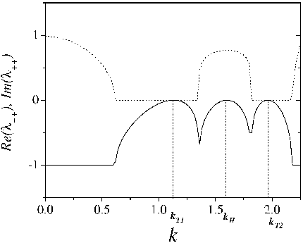
Taking an adequate value of , it is possible to make unstable wavenumbers fulfill the desired ratio. Simulations with were performed. For some parameters, dominated and a regular dodecagon took place in the far field. Finally, putting an initial condition that was the steady solution plus an hexagonal pattern related to the smallest wavenumber, it could be seen that both unstable wavenumbers grew, forming an organized hexagonal structure in the near and in the far field. The same result was found even when the input intensity was slightly lower than critical intensity. See Fig. 9, where, for , the coexistence of two unstable wavenumbers can be found even in the near field. The stability analysis for this case is shown in Fig 9: it can be seen that there are 2 unstable wavenumbers, i.e. two values of for which is not negative.

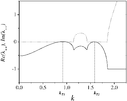
Codimension 3 situations were also analyzed. Parameters were chosen so that the ratio between the greatest Turing wavelength and the smallest one was (). At the initial stage, we found that all unstable wavenumbers where activated (see the left plot on fig. 11), forming three concentric circumferences in the far field. The smallest Turing wavenumber grew faster, and turned into an hexagon. After that, another hexagon, related to the greatest Turing wavenumber also appeared, see Fig. 11 middle plot. At odds with fig. 9, regions where instabilities with different wavenumbers dominate are spatially separate in the near field. Finally, a crown of modes got destabilized (right plot on fig. 11). The stability analysis for this case is shown in Fig 11. Notice that the intermediate unstable wavenumber is related to Hopf instability, i.e. it has .

In another example of resonant Turing-Hopf-Turing Codimension 3, in which , a similar final situation was observed. For nonresonant cases, there were found steady situations similar to fig. 11, middle graph, but where one Turing wavevector (making an hexagon or a ring in the far field) prevailed for but the other prevailed for .
For Turing Hopf codimension 2, situations similar to Turing Turing codimension 2 were found, both in resonant and nonresonant situations. Also, square patterns took place in some numerical integrations.
IX Conclusions
Taking into account the polarization degree of freedom of light, and having in mind that , which measures the nonlinear coupling between different polarizations, could take a broad range of values, we presented a study of instabilities and patterns that might show up in a cavity filled with a Kerr-like nonlinear material with positive or negative refractive index.
A method for finding codimension 2 and 3 situations (where wavenumbers of different modulus might destabilize) was shown. It can be found that for Turing-Turing codimension 2 may occur; for , Turing-Hopf-Turing codimension 3 may take place, and for there may be situations for Turing-Hopf codimension 2. Fixing only the value of , the method allows us to find all other values of the parameters for codimension 2 or 3. It allows also to see that, for a given intensity, there cannot be more that three instability regions in a marginal instability plot (one of which has to be related to a Hopf instability), and that codimension higher than 3 cannot occur.
Since the method allows us to know some parameters with any degree of precision (instead of performing a numerical search and changing the parameters until such situation shows up), and choose others at will, it is a useful tool in the study of codimension 2 or 3 on the model. Specifically, resonant situations, where the ratios between unstable wavevectors are chosen, can be found. Also, it might be useful for the underestanding of pattern formation in other systems as long as the linear stability analysis presents eigenvalues with the form of eqs. (6) and (7).
Numerical integration results show some new situations of pattern coexistence and competition.
Acknowledgments
This work was partially supported by Consejo Nacional de Investigaciones Científicas y Técnicas (CONICET, Argentina, PIP 0041 2010-2012).
Appendix A: Properties of instability tongues
We consider that the possible values are those given by these polynomials with the free parameter , and with fixed coefficients, i.e., we consider fixed values of and , that correspond to a fixed value of the input intensity for a determined homogeneous solution. From (7) we see that takes a maximum value given by . By definition, , so it can be shown that , and that for . This means that, for large , . Therefore, the range of unstable wavenumbers is bounded. The case occurs only if , that is, for pure circular polarization, but this case can be related to the pure linear polarization case, as has been done, for instance in [3].
From (7), we can obtain two solutions for as a function of . Using these solutions in the equation for , we obtain:
| (A.1) |
where and ; indices ‘u’ and ‘l’ stand for upper and lower curves respectively.
The difference between the upper and lower curves is . So, we have two values of for each as long as and . For , the curves are two overlapping rays that start from . We can also see that , so () has negative (positive) curvature.
To obtain the instability points, we have to look at the intersection of with the unstable regions of Fig. 4. Eq. (A.1) can be rewritten as:
| (A.2) |
where (the same equation holds for and ). To obtain the intersection with the stationary unstable region, we replace by in (A.2). We get a 4th order polynomial, so there are at most 4 solutions for . The intersection with the oscillatory unstable region is obtained replacing by in (A.2); this gives two solutions for . To obtain the maximum number of unstable ranges of values of we assume that half of the previously mentioned solutions of correspond to a cross from stable to unstable region (as is increased) and the other half to a cross from unstable to stable region. So, we have, at most, three unstable ranges of that correspond to three tongues in the marginal stability diagrams.
Appendix B: Derivation of parameters valid for codimension 2 and 3
For Turing-Turing codimension 2, we need both and to be tangent to the border of the stationary unstable region, and this happens only if ; in this case and are straight lines that overlap. To have codimension 3 (Turing-Hopf-Turing) there is a further condition: the end point of the rays, , must be on the border of the oscillatory unstable region given by . The case of Turing-Hopf codimension 2 occurs when against is tangent to the borders of the stationary and oscillatory unstable regions, and . See Fig. 6.
Turing-Turing codimension 2 and Turing-Hopf-Turing codimension 3
From the condition it is straightforward to obtain an expression for , (10). From Eq. (A.2) we have that , and the intersection with the border of the stationary unstable region, given by , gives a 2nd order polynomial in . To have the line tangent to the parabola, the discriminant of the polynomial should be zero. From this conditions we get the critical value from which, using Eq. (7), we get the two critical values of . From the zero discriminant and Eq. (10), we get an expression for , (9).
Then, for a given value of , there is a unique value of and where we can find Turing-Turing codimension 2. There are some restrictions on the possible values of . First, in order to have real, we have that , but there is a more restrictive condition. We need that in order to have a solution tangent to the unstable border that actually touches it. It can be shown that the condition should be satisfied. Second, the Hopf instability should appear for greater values of than the Turing-Turing instability.
We define the distance between and the border of the oscillatory unstable region as . For Turing-Turing codimension 2 we need , and for codimension 3, we have that since the point should be on the oscillatory unstable border. Since and are functions of [see Eqs. (9) and (10)], we can obtain as a function of only. It can be shown that the only zero of Z occurs for . Then, using the value , we can obtain the parameters and for codimension 3. For , , so that Turing-Turing codimension 2 is allowed. For , : we still have the two stationary instabilities that occur simultaneously for a given value of , but this is not Turing-Turing codimension 2 since the oscillatory instability appears for a smaller value of (As we will see below, in that region there are Turing-Hopf instabilities).
Expressions for and can be found solving , and replacing by and by . If there is codimension 3, the value of can be found from . It can be shown that . Once the value of is chosen, , and are fixed. Conversely, once two wavenumbers are chosen, is fixed (and so is the third wavenumber, if exists).
Turing-Hopf codimension 2
For a Turing-Hopf codimension 2 we require the curve to be tangent to both borders of the unstable regions, as shown in the lower row of Fig. 6.
Let us first consider the contact point with the border of the oscillatory unstable region, i.e., between (A.1) and the line . The intersections are given by a second order polynomial in . We require the intersection to be only in one point, so that the polynomial discriminant should be zero. From this condition, it is possible to obtain three possible expressions for as a function of and . We will call them .
Now, we consider the intersection with the stationary unstable region, i.e., between and . We get a fourth order polynomial in , which will be called . We can have 0, 2 or 4 real roots, and we are interested in the cases of a fourfold real root, or double real and two complex conjugate roots, in order to have the function tangent to the unstable border. It can be shown that the kind of roots that we are looking for are possible only for one of the expressions of mentioned in the previous paragraph, say . In fig. 7 we plot the roots of . Its coefficients are calculated for , and .
The value of can be found solving , where is the double root of . The value of can be found in a similar way.
Bibliography
References
- [1] L. A. Lugiato, M. Brambilla, A. Gatti, Optical pattern fomation, Advances in Atomic, Molecular and Optical Physics 40 (1999) 229.
- [2] K. Staliunas, V.J. Sanchez-Morcillo, Transverse Patterns in Nonlinear Optical Resonators, Springer Verlag, Springer Tracts in Modern Physics, Vol.183, 2003.
- [3] M. Hoyuelos, P. Colet, M. San Miguel, D. Walgraef, Polarization patterns in Kerr media, Phys. Rev. E 58 (1998) 2992.
- [4] V. Yannopapas, Enhancement of nonlinear susceptibilities near plasmonic metamaterials, Opt. Commun. 283 (2010) 1647.
- [5] J. E. Sipe, R. W. Boyd, Nonlinear susceptibility of composite optical materials in the Maxwell Garnett model, Phys. Rev. A 46 (1992) 1614.
- [6] S. A. Ramakrishna, Physics of negative refractive index materials, Rep. Prog. Phys. 68 (2005) 449.
- [7] R. Merlin, Metamaterials and the LandauLifshitz permeability argument: Large permittivity begets highfrequency magnetism, PNAS 106 (2009) 1693-1698.
- [8] A. A. Zharov, I. V. Shadrivov, Y. S. Kivshar, Nonlinear Properties of Left-Handed Metamaterials, Phys. Rev. Lett. 91 (2003) 037401.
- [9] R. Morandotti, H. S. Eisenberg, Y. Silberberg, M. Sorel, J. S. Aitchison, Self-Focusing and Defocusing in Waveguide Arrays, Phys. Rev. Lett. 86 (2001) 3296.
- [10] K. Staliunas, R. Herrero, Nondiffractive propagation of light in photonic crystals, Phys. Rev. E 73 ͑(2006͒) 016601.
- [11] Staliunas, O. Egorov, Y. S. Kivshar, F. Lederer, Bloch Cavity Solitons in Nonlinear Resonators with Intracavity Photonic Crystals Phys. Rev. Lett. 101, 153903 (2008)
- [12] D. A. Martin, M. Hoyuelos, Homogeneous solutions for elliptically polarized light in a cavity containing materials with electric and magnetic nonlinearities, Phys. Rev. A 82 (2010) 033841.
- [13] P. Tassin, G. Van der Sande, I. Veretennicoff, M. Tlidi, P. Kockaert, Analytical model for the optical propagation in a nonlinear left-handed material, Proc. SPIE 5955 (2005) 59550X.
- [14] D. A. Martin, M. Hoyuelos, Cavity equations for a positive- or negative-refraction-index material with electric and magnetic nonlinearities, Phys. Rev. E 80 (2009) 056601.
- [15] L. A. Lugiato, R. Lefever, Spatial Dissipative Structures in Passive Optical Systems, Phys. Rev. Lett. 58 (1987) 2209.
- [16] R. W. Boyd, Nonlinear Optics, third ed., Academic, New York, 2007.
- [17] J. Bugin, C. Gillon, P. Langot, Femtosecond investigation of the non-instantaneous third-order nonlinear suceptibility in liquids and glasses, Appl. Phys. Lett. 87 (2005) 211916.
- [18] A. J. Scroggie, W. J. Firth, G. S. McDonald, Pattern formation in a passive Kerr cavity, Chaos, Solitons & Fractals 4 (1994) 1323.
- [19] D. Gomila, P. Colet, Transition from hexagons to optical turbulence, Phys. Rev. A 68 (2003) 011801.
- [20] M. C. Cross, P. C. Hohenberg, Pattern Formation Out of Equilibrium, Rev. Mod. Phys. 65 (1993) 851.
- [21] M. Hoyuelos, D. Walgraef, P. Colet, M. San Miguel, Patterns arising from the interaction between scalar and vectorial instabilities in two-photon resonant Kerr cavities, Phys. Rev. E 65 (2002) 046620.
- [22] L. Yang, M. Dolnik, A. M. Zhabotinsky, I. R. Epstein, Pattern formation arising from interactions between Turing and wave instabilities, J. Chem. Phys.117 (2002) 7259.
- [23] M. Meixner, S. Bose, E. Scholl, Analysis of complex and chaotic patterns near a codimension-2 Turing-Hopf point in a reaction-diffusion model, Physica D 109 (1997) 128-138.
- [24] B. Thüring, A. Schreider, M.Kreuzer, T. Tschudi, Spatio-temporal dynamics due to competing spatial instabilities in a coupled LCLV feedback system, Physica D 96 (1996) 282-290.
- [25] B. Y. Rubinstein, L. M. Pismen, Resonant patterns in a two-component optical system with 2-D feedback, Opt. Commun. 145 (1998) 159-165.
- [26] I.P. Nikolaev, A.V. Larichev, E.V. Degtiarev, V. Wataghin, An optical feedback nonlinear system with a Takens-Bogdanov point: experimental investigation, Physica D 144 (2000) 221-229.
- [27] Numerical integrations were performed in a 256 by 256 square matrix, with periodic boundary conditions. Evolution was calculated with a fourth order Runge Kutta method. Time step was .