Nature of the many-body excitations in a quantum wire: theory and experiment
Abstract
The natural excitations of an interacting one-dimensional system at low energy are hydrodynamic modes of Luttinger liquid, protected by the Lorentz invariance of the linear dispersion. We show that beyond low energies, where quadratic dispersion reduces the symmetry to Galilean, the main character of the many-body excitations changes into a hierarchy: calculations of dynamic correlation functions for fermions (without spin) show that the spectral weights of the excitations are proportional to powers of , where is a length-scale related to interactions and is the system length. Thus only small numbers of excitations carry the principal spectral power in representative regions on the energy-momentum planes. We have analysed the spectral function in detail and have shown that the first-level (strongest) excitations form a mode with parabolic dispersion, like that of a renormalised single particle. The second-level excitations produce a singular power-law line shape to the first-level mode and multiple power-laws at the spectral edge. We have illustrated crossover to Luttinger liquid at low energy by calculating the local density of state through all energy scales: from linear to non-linear, and to above the chemical potential energies. In order to test this model, we have carried out experiments to measure momentum-resolved tunnelling of electrons (fermions with spin) from/to a wire formed within a GaAs heterostructure. We observe well-resolved spin-charge separation at low energy with appreciable interaction strength and only a parabolic dispersion of the first-level mode at higher energies. We find structure resembling the second-level excitations, which dies away rapidly at high momentum in line with the theoretical predictions here.
pacs
71.10.Pm, 03.75.Kk, 73.63.Nm, 73.90.+fI Introduction
Predicting the behaviour of interacting electrons is a significant open problem. Most progress to date has been made at low energies where linearisation of the single-particle dispersion led to construction of Fermi[1] and, in one dimension, to Luttinger-liquid theories[2] in which the natural excitations are fermionic quasiparticles and hydrodynamic modes respectively. The only significant progress beyond the linear approximation has been achieved via the heavy impurity model, for Fermi[3, 4, 5] and Luttinger[6] liquids, showcasing threshold singularities drastically different from the low energy behaviour. In this paper we investigate one-dimensional (1D) fermions beyond the linear approximation where the natural many-body excitations form a hierarchical structure,[7] in sharp contrast with the Fermi quasiparticles or hydrodynamic modes. We obtain the dynamical structure factor, in addition to the already known spectral function, and construct an inductive proof for calculating the form factors that are necessary for the dynamical response functions of the spinless fermion model. Experimentally, we demonstrate control over the interaction energy a 1D wire manifested as a change of the ratio of the charge and spin velocities at low energy scales. We find a new structure resembling the second-level excitations, which dies rapidly away from the first-level mode in a manner consistent with a power law.

We analyse theoretically the dynamic response functions–that probe the many-body excitations–for spinless fermions with short-range interactions. Our approach is exact diagonalisation via Bethe ansatz methods: the eigenenergies are evaluated in the coordinate representation and form factors–for the corresponding eigenstates–are derived in the algebraic representation, via Slavnov’s formula.[8] On the microscopic level the excitations arrange themselves into a hierarchy via their spectral weights–given by the form factors–with different powers of , where is the particle-particle interaction radius and is the length of the system. As a result only small numbers of states–out of an exponentially large Fock space of the many-body system–carry the principal spectral power in representative regions on the energy-momentum plane, see Fig. 1, allowing an analytical evaluation of the observables.
At small energy this hierarchy crosses over to hydrodynamic behaviour, see Fig. 1, that we illustrate by calculating the local density of states. At low energy it is suppressed in a power-law fashion according to the Tomonaga-Luttinger theory. Away from the Fermi point where the Lorentz invariance is reduced to Galilean by the parabolicity of the spectrum, the local density of states is dominated by the first(leading)-level excitations of the hierarchy. This produces a van Hove singularity, where is the energy measured from the bottom of the conduction band. At even higher energies the second-level excitations produce another van Hove singularity on the other side of the band edge, in the forbidden for the non-interacting system region.
Using this framework, we study response of the correlated system to adding/removing a particle in detail, given by the spectral function. The first-level excitations form a parabolic dispersion, like a single particle, with a mass renormalised by the Luttinger parameter . [9] The continuous spectrum of the second-level excitations produces a power-law line-shape around the first-level mode with a singular exponent . Around the spectral edges the second-level excitations give a power-law behaviour of the spectral function. For the hole edge the exponent calculated microscopically reproduces the prediction of the phenomenological heavy impurity model in one-dimension.[6] However, around the particle edge the second-level excitations give a power-law of a new type.
Experimentally, momentum-resolved tunneling of electrons confined to a 1D geometry has been used to probe spin-charge separation in a Luttinger liquid.[11, 12, 38, 39] This separation was observed to persist far beyond the energy range for which the Luttinger approximation is valid,[12] showing the need for more sophisticated theories.[37] Particle-hole asymmetry has also been detected in relaxation processes.[10] In this paper we measure momentum-resolved tunneling of electrons in the upper layer of a GaAs-AlGaAs double-quantum-well structure from/to a 2D electron gas in the lower layer. This set-up probes the spectral function for spinful fermions. We observe well-resolved spin-charge separation at low energy with appreciable interaction strength—a distinct effect of the spinful generalisation of Luttinger liquid.[2] The ratio of charge and spin velocities is .[12] At high energy, in addition to the spin and charge curves, we can also resolve structure just above that appears to be the edge of the second-level excitations. However, the amplitude decays rapidly and for higher we find no sign of the higher-level excitations, implying that their amplitude must have become at least three orders of magnitude weaker than for the parabola formed by the first-level excitations. The picture emerging out of these experimental results can only be explained—though only qualitatively—by the hierarchy that we study for spinless fermions.
The rest of the paper is organised as follows. In Section II we describe the one-dimensional model of interacting spinless fermions introducing a short range cut-off via lattice. Section III contains a procedure of finding the many-body eigenenergy by means of the coordinate Bethe ansatz. In Section IV we evaluate the form factors needed for the dynamical response functions. We give a construction of the algebraic representation of Bethe ansatz (Subsection IVa) and evaluate the scalar product in this representation (Subsection IVb). We present a calculation of the form factors for the spectral function and the dynamical structure factor for a finite chain (Section IVc). We take the limit of long wavelengths deriving polynomial formulae for the form factors (Subsection IVd). Then, we analyse the obtained form factors establishing hierarchy of excitations (Subsection IVe). Finally we calculate the spectral function around the spectral edges (Subsection IVf). In Section V we illustrate the crossover to Luttinger liquid at low energy by evaluating the local density of states at all energy scales. Section VI describes experiments on momentum-conserved tunnelling of electrons in semiconductor wires. Section VII is dedicated to low energies and in Section VIII we analyse the measurements at high energies connecting the experiment with theory on spinless fermions developed in this paper. Figures below are marked with spinless and spinful logos (such as those in Fig. 2 and 7, respectively) to indicate the structure of the paper visually. Appendix A contains details of the derivation of the Bethe equations in the algebraic representation. In Appendix B we derive the expectation value of the local density operator.
II Model of spinless fermions
We study theoretically the model of interacting Fermi particles without spin in 1D,
| (1) |
where the field operators satisfy the Fermi commutation relations, , is the particle density operator, and is the bare mass of a single particle. Below we consider periodic boundary conditions, , restrict ourselves to repulsive interaction only, and take .
Non-zero matrix elements of the interaction term in Eq. (1) require a finite range of the potential profile for Fermi particles. Here, we will introduce a lattice with next-neighbour interaction which lattice parameter and interaction radius is . The model in Eq. (1) becomes
| (2) |
where is the site index on the lattice, the dimensionless length of the system is , the operators obey , and .
The long wavelength limit of the discrete model corresponds to the model in Eq. (1) while the interaction radius provides microscopically an ultraviolet cutoff in the continuum regime. For -particle states of the lattice model we additionally impose the constraint of low particle density, , to stay within the conducting regime; a large occupancy might lead to Wigner crystal physics at sufficiently strong interactions that would localise the system. This procedure is analogous to the point splitting regularisation technique [15] which is usually introduced within the framework of the Luttinger liquid mode in the linear regime.
III Spectral properties
The model in Eq. (2) can be diagonalised via the Bethe ansatz approach which is based on the observation that the eigenstates are superpositions of plain waves. This method is also called coordinate Bethe ansatz.[13] The eigenstates, following Ref. 13, can be parameterised with sets of quasimomenta ,
| (3) |
Their corresponding eigenenergies, , are Here is the vacuum state, the scattering phases are fixed by the two-body scattering problem,
| (4) |
and is a sum over all permutation of quasimomenta. The periodic boundary condition quantises the whole set of quasimomenta simultaneously,
| (5) |
where are sets of non-equal integer numbers.
Generally, the system of equations in Eq. (5) has to be solved numerically to obtain the full spectral structure of the observables. However, in the long-wavelength regime the solutions can be evaluated explicitly.
In this limit the scattering phases in Eq. (4) are linear functions of quasimomenta, , which makes the non-linear system of Bethe ansatz equations in Eq. (5) a linear system.[9] Then, solving the linear system for via the matrix perturbation theory up to the first subleading order in we obtain
| (6) |
Note that this calculation is valid for any interaction strength at low densities. The corresponding eigenenergy and total momentum (protected by the translational invariance of the system) are
| (7) |
and .
The spectrum of the many body states is governed by the first term in Eq. (6). Reduction of the quantisation length in the denominator of the first term in Eq. (6) is an exclusion volume taken by the sum of interaction radii of all particles. Thus all -particle eigenstates at an arbitrary interaction strength are given straightforwardly by the same sets of integer numbers as the free fermions’ states, e.g. the ground state corresponds to .
For example, this result can be used to calculate the low energy excitations explicitly that define the input parameters of the Luttinger-liquid model, the velocity of the sound wave and of the Luttinger parameter . The first pair of the particle-like excitations, when an extra electron is added just above the Fermi energy, have and . The difference in their energies and momenta are and . Evaluating the discrete derivative, which gives the slope of the dispersion around the Fermi energy, as we obtain
| (8) |
where is the Fermi velocity and the relation between the Luttinger parameters for Galilean invariant systems[14] was used.
IV matrix elements
Now we turn to calculation of matrix elements. But first we need to select operators that corresponds to specific observables. Our interest lies in the dynamical response functions that correspond to adding/removing a single particle to/from a correlated system and to creating an electron-hole pair excitation out of the ground state of a correlated system. For example, the first type of dynamics can be realised in experiments using semiconductor nano-structures[11, 12] where an electrical current, generated by electrons tunnelling into/from the nano-structure with their momentum and energy under controlled, probes the system.
The response of the many-body system to a single-particle excitation at momentum and energy is described by spectral function[16] . Here is the chemical potential and is Green function at zero temperature. In terms of the eigenstates the spectral function reads
| (9) |
where is the energy of the ground state , and and are the momenta and the eigenenergies of the eigenstates ; all eigenstates are assumed normalised.
Creation of an electron-hole pair out of the correlated state at zero temperature at momentum and energy is described by dynamical structure factor[16] , where is the density operator evolving under the Hamiltonian to time and the average is taken over the ground state. In term of the eigenstates the dynamical structure factor reads
| (10) |
Thus, we will be analysing the expectation values of the local operators and . To proceed with this calculation we will borrow the result from Ref. 17, 18 for Heisenberg chains. Our strategy is to perform the full calculation for the discrete model in Eq. (2) obtaining the matrix elements of and as determinants. Then we will take the long wavelength limit to evaluate the form factors for the continuum model explicitly which will be the main technical result in the theoretical part of this paper. Below we will construct the algebraic form of Bethe ansatz, use the Slavnov’s formula[8] to express the scalar product and the normalisation factors in this representation, and finally calculate the matrix elements of the local operators.
IV.1 Algebraic Bethe ansatz
The wave function of the -particle eigenstates are factorised in the algebraic representation which allows the general calculation of various scalar products between them. Here we will follow the construction in Ref. 13 for XXZ spins chains changing basis from 1/2-spins to spinless fermions.
The so called -matrix acts on a tensor product space and depends on an auxiliary parameter , where and are element-element subspaces each of which consists of two states and . It is a solution of Yang-Baxter equation . For the lattice model in Eq. (2) the -matrix reads
| (11) |
where
| (12) |
Here is the interaction parameter, and the tensor product space is defined using fermionic basis and with corresponding fermionic operators that act in these bases as . The latter will account for anticommuting nature of the lattice fermions on different sites in contrast to the commutation relation of the spin operators of a spin chain model.[22, 23] All further calculation are identical to spin chains where the anti-commutation relations of the Fermi particles are however automatically fulfilled. This approach is more convenient than direct mapping of the results for spin chains using Jordan-Wigner transformation.[19]
A two-states subspace of -matrix can be identified with the two-states fermionic subspace of the lattice site of the model in Eq. (2). Then, the quantum version of the Lax operator (the so called -matrix) can be defined as . In the auxiliary subspace its matrix and operator forms are
| (13) |
Here the top left element element of the matrix is a transition between and states of the auxiliary subspace, and are the fermionic operators of the lattice model in Eq. (2), and label the matrix elements of . The prefactor in front of was chosen such that for it becomes a permutation matrix and for the -operator is diagonal.
By construction the -operator satisfies algebra generated by Yang-Baxter equation,
| (14) |
The entries give commutation relations between the matrix elements of -matrix. Here we write down three of them that will be used later,
| (15) |
| (16) |
| (17) |
These relations can be also be checked explicitly by direct use of the definition in Eq. (13) and the Fermi commutation relations.
The transition matrix for a chain with sites–the so called monodromy matrix–can be defined similarly to the classical problem as
| (18) |
If all single-site -matrices satisfy Eq. (14) then the -matrix also satisfies the same Yang-Baxter equation, e.g. see proof in Ref. 13. Therefore the matrix elements of in the 2x2 auxiliary space obey the same commutation relations in Eqs. (15-17). The transfer matrix for the whole chain,
| (19) |
is the super trace of -matrix due to the fermionic definition of the auxiliary space.[22, 23] The latter gives a family of commuting matrices , which contain all conserved quantities of the problem including the Hamiltonian.
The vacuum state –in the Fock space of the model in Eq. (2)–is an eigenstate of the transfer matrix . The corresponding eigenvalue, , is the difference of the eigenvalues of the and operators which can be obtained directly by use of the definitions in Eqs. (13, 18). Noting that for Eq. (18) gives and , where and , and generalising this observation for arbitrary one obtains
| (20) |
A general state of particles’–Bethe state–is constructed by applying the operator times with different values of the auxiliary variable ,
| (21) |
where a set of values corresponds to quasimomenta in coordinate representation of Bethe states in Eq. (3). The state in Eq. (21) with an arbitrary set of is not an eigenstate of the transfer matrix . For instance, it can be seen by commuting the operators and from left to right through all operators that generates many different states according to the commutation relations in Eqs. (16,17). However the contribution of all of the states that are non-degenerate with can made to be zero by choosing particular sets of that satisfy the following set of equations
| (22) |
(see Appendix A for details).
Under the substitution of the vacuum eigenvalues and of and operators from Eq. (20) and – which define the commutation relations Eqs. (16,17) – from Eq. (12) this so called eigenvalue equation above becomes
| (23) |
Thus all the sets of that satisfy the above equation give eigenstates of the transfer matrix in the representation of Eq. (21) with the corresponding eigenvalues where
| (24) |
This eigenvalue equation in the algebraic framework is the direct analog of the Bethe ansatz equation (5) in the coordinate representation. Direct mapping between the two is done by the substitution of
| (25) |
in Eq. (5) and by taking its exponential.
!The original lattice Hamiltonian can be obtained from the transfer matrix that contains all of the conserved quantities of the problem. Logarithmic derivatives of give the global conservation laws by means of the so called trace identities, see Ref. 13. The linear coefficient in the Taylor series around the point is proportional to the Hamiltonian itself. After restoring the correct prefactor the expression reads
| (26) |
Substitution of the interaction parameter from Eq. (25) in terms of the particle-particle interaction constant, , in to the right hand side of the above relation recovers the lattice model in Eq. (2).
IV.2 Scalar product
The basic quantity, which calculations of expectation values will be based on, is the scalar product of two wave functions. A general way of evaluating it is the commutation relations in Eqs. (15-17) and the vacuum expectation values of the and operators. The result of such a calculation simplifies greatly if one of the Bethe states is an eigenstate of the transfer matrix , as was first shown by Slavnov.[8] Then the same result was rederived in Ref. 17, 18 using the so-called factorising -matrix,[20] which is a representation of a Drinfeld twist.[21] The latter will not be used in this Subsection but it will be needed later in calculations of the matrix elements of the local operators.
Let be an eigenstate of the transfer matrix so that parameters satisfy the Bethe equation in Eq. (23). And let be another Bethe state parametrised by a set of arbitrary values . The scalar product of these two states can be evaluated by commuting each operator though the product of operators using the commutation relation in Eq. (15), which generates the and operators with all possible values of and . They, in turn, have also to be commuted to the right through the remaining products of the operators. Finally products of the and operators, which act upon the vacuum state, just give products of their vacuum eigenvalues and according to Eq. (20). The resulting sums of products can be written, using the relation between in Eq. (23), in a compact form as a determinant of an matrix[8]
| (27) |
where the matrix elements are . Under substitution of the eigenvalues of the transfer matrix from Eq. (24) these matrix elements read in explicit form as
| (28) |
For the result in Eqs. (27, 28) follows directly from Eq. (15). For arbitrary the proof is more complicated: it employs the residue formula[8] (the function has first order poles when ) and the recurrent relation for the scalar product of particles in terms of the scalar product of particles, see also details in Ref. 13.
The normalisation factor of Bethe states can be obtained from Eq. (27) by taking the limit . The first order singularities, , in the off-diagonal matrix elements Eq. (28) are cancelled by zeros in the numerator in Eq. (27). The diagonal matrix elements contain second order singularities for . However, the numerator also becomes zero when in the leading order. Its expansion up to the first subleading order cancels the second order singularity of the denominator giving a finite expression for the matrix elements in the limit. The normalisation factor is found to be
| (29) |
where the matrix elements are
| (30) |
The last formula was originally derived by Gaudin using quantum mechanical identities in the coordinate representation of Bethe ansatz.[24] Mapping of the resulting expression in Ref. 24 to the algebraic representation by means of Eq. (25) gives directly the result in Eqs. (27, 28) with a different prefactors due to different normalisation factors in the definitions of the states in Eq. (3) and of the states in Eq. (21). We will use the algebraic form in Eq. (21) for the calculation of the local matrix elements below.
IV.3 Expectation values of local operators
Operators of the algebraic Bethe ansatz in Eqs. (13, 18) are non-local in the basis of the original fermionic operators of the lattice model in Eq. (2). Thus, the first non-trivial problem in calculating the matrix elements of the local operators and in the algebraic representation of Bethe states in Eq. (21) is expressing the operators of our interest in terms of the non-local and operators from Eqs. (13, 18). Alternatively these Bethe operators can be expressed in terms of the local operators of the lattice model. The latter approach is much more complicated since the product of matrices in Eq. (18) is a large sum (exponential in the number of sites in the chain) restricting severely the ability to do explicit calculations using the fermionic representation in practice.
An alternative way was found by constructing the -matrix representation of a Drinfeld twist.[20] In the -basis the monodromy matrix in Eq. (18) becomes quasi-local, i.e. its diagonal elements and become direct products of diagonal matrices on each site over all sites of the chain and the off-diagonal and are single sums over such direct products. Direct calculations become much easier in this basis. Specifically, analysis of operators leads to a simple result for representing the operator in terms of algebraic Bethe ansatz operators, which then is shown to be basis independent,[17, 18]
| (31) |
Here is the super trace of the monodromy matrix and is its matrix element.
The transfer matrices in the right hand side of the above equation give only a phase prefactor in the expectation values with respect to the Bethe states in Eq. (21). Let be an eigenstate of the transfer matrix with particles, let be an eigenstate with particles, and let us consider the case of . Acting with the operator on the eigenstates gives the eigenvalue according to Eq. (24). Then, using the mapping to the coordinate representation in Eq. (25) and the Bethe equation in the form of Eq. (5), this eigenvalue can be expressed as where is the total momentum of the state , a quantum number. Similar phase factors for are evaluated in an analogous way and each of them cancels out under modulus square in the form factor in Eq. (9) making the local form factors independent of in full accord with the translational invariance of the system and the observable in Eq.(9). Thus we will only calculate the value of .
Since is also a Bethe state , though it is not an eigenstate, the expectation value can be calculated using the result for the scalar product . Substituting in Eqs. (27,28) explicitly one obtains
| (32) |
where the matrix elements are
| (33) |
for , and
| (34) |
for . Here the Bethe equation in Eq. (23) was used to express in the matrix elements, and some factors in the matrix elements and the overall prefactor cancel out. This result can be checked by numerical evaluation of the sums over spacial variables using the coordinate representation in Eq. (3) for a small number of particles which we have done.
The determinant results in Eqs. (29, 27, 32) can be checked by numerical evaluation of the sums over spacial variables using the coordinate representation in Eq. (3). However the latter summation over many coordinates has factorial complexity which already limits numerical calculations to a few particles on chains of a few dozens sites. The results of the algebraic Bethe ansatz calculations have a power-law complexity that allows general studies, at least numerically, of systems with hundreds of particles on arbitrary long chains without making any approximations, e.g. the studies of correlation functions in one-dimensional systems in Refs. 25, 26, 27, 28, 29, 30.
IV.4 The long wavelength limit
We now turn to the evaluation of the long wavelength limit for matrix elements in the determinant form with the aim of calculating the determinants explicitly. The resulting expressions will then be used to study physical observables.
Such an analysis is more convenient in the coordinate representation. For small the non-linear mapping in Eq. (25) becomes linear, similarly to Bethe equation in Eq. (5) in this limit. Then, a simple inversion of the linear function gives
| (35) |
Note that and are simultaneously much smaller than one, while the interaction strength can be of an arbitrary magnitude.
We start from the expansion of the normalisation factor in Eq. (29) up to the leading non-vanishing order in the quasimomenta. We first substitute Eq. (35) in the matrix elements in Eqs. (30), then expand them up the leading non-vanishing order in , and obtain the diagonal matrix elements as follows,
| (36) |
and
| (37) |
for . The off-diagonal matrix elements are small compared to the diagonal entries as so the leading contribution to the determinant is accumulated on the diagonal. Also expanding the prefactor of Eq. (29) in small we obtain the following expression for the normalisation in the long wavelength limit,
| (38) |
where are quasimomenta in the coordinate representation of Bethe ansatz.
Our primary interest lies in the spectral function which contains the local matrix element of operators so here we will focus on the determinant result in Eq. (32). Similarly to the calculation of the normalisation factor we substitute Eq. (35) into Eq. (33), which however becomes zero in the zeroth order in . Expanding it up to linear order in we obtain
| (39) |
for , where is the difference of two conserved quantities, the momenta of two states and . The matrix elements in Eq. (34) are already non-zero in the zeroth order in giving
| (40) |
for . Also expanding the prefactor in Eq. (32) and rearranging the expressions by taking a common factor out of the matrix elements we obtain
| (41) |
where the entries of the matrix under the determinant, , for are
| (42) |
All matrix elements are of the the same order so the determinant in Eq. (41) is a sum of a large number of terms unlike the normalisation factor in Eq. (38). Doing the summation we find an explicit expression in the form of a fraction of two polynomials in quasimomenta of the initial and the final states,
| (43) |
For the result above is evaluated straightforwardly as a determinant of a matrix with the matrix elements in Eq. (42). For arbitrary we prove it by induction. Using the Laplace development on the row, the determinant for particles can be expressed as a sum of minors given, in turn, by determinants for particles, , which – let us assume for purposes of the inductive method – are given by Eq. (43)
| (44) |
Here are given by the matrix elements in Eq. (42), quasimomenta are labeled by , and quasimomenta are labeled by with elements excluded. Under taking common factor in front of the sum, the determinant for particles becomes
| (45) |
The sum in the above expression gives, by direct calculation, which makes the whole second line unity. The determinant is equal to the first line of Eq. (45) which is also equal to the result in Eq. (43) for particles. Thus we obtained the same result for particles starting from Eq. (43) for particles. Hence, it is proved by induction.
Finally, the form factor in the Eq. (9) is the modulus squared of Eq. (41). Normalising the initial and the final state wave functions using Eq. (38) as we obtain
| (46) |
where , and are the quasimomenta of the eigenstate and the ground state , and for the ground state.
Calculation of is done in a similar way by expressing the local density operator , within the framework of the lattice model, in terms of the algebraic Bethe ansatz operators , , , and, then, by using the Slavnov formula. Details are given in appendix B. In the long wavelength limit we obtain
| (47) |
where the final states have the same number of excitations as the ground state , unlike in Eq. (46), and for the ground state as in Eq. (46).
These form factors in Eqs. (46, 47) together with the solution of Bethe equations in Eq. (6) is the main technical result in the theory part of our work. We will analyse its physical consequences in the next two Subsections. The similarity between these two expressions means that the hierarchy of modes we will identify below is a general feature of one and two body operators.
IV.5 Hierarchy of modes
The results in Eqs. (46, 47) have one or more singularities when one or more quasimomenta of an excited state coincide with a quasimomentum of the ground state, . Both results have a multiplicand that becomes virtually zero in the thermodynamic limit, in which . Thus the product of these two opposite factors produces an uncertainty in the limiting behaviour (of the type) that has to be resolved. Since we are specifically interested in a transport experiment in this paper, in which the spectral function is measured, we will mainly focus on solving the uncertainty problem for result in Eq. (46).

The maximum number of singularities is in the extreme case, when quasimomenta of an excited state coincide with all of the quasimomenta of the ground state given in Fig. 2gs. The excited states of this kind are given in Fig. 2a. The divergences in the denominator of Eq. (46) occur only in the leading order—the first term in Eq. (6)—but the subleading order—the second term in Eq. (6)—already provides a self-consistent cutoff within the theory. The interaction shift of the quasimomenta at subleading order does not cancel for the extra added particle in the excited state, making the factors in the denominator of Eq. (46)
| (48) |
where in the r.h.s. only the first term from Eq. (6) is relevant for and . The numerator for the states in Fig. 2a becomes
| (49) |
Substitution of Eqs. (48, 49) in Eq. (46) for one particle, say for , cancels one factor and the other part of the product for in the denominator of first line of Eq. (46) cancels partially the products in the second line of Eq. (46). The expression for the remaining particles is the same as Eq. (46) but the numbers of terms in the products are reduced by one, , giving
| (50) |
Repeating the procedure times we cancel the remaining factor completely (with the rest of other terms) and obtain
| (51) |
Corrections to this result originate from higher subleading orders in the solutions to Bethe equations in Eq. (6) and are of the order of . This becomes much smaller than one at leading order of Eq. (51) in the thermodynamic limit.
Substitution of Eq. (51) in Eq. (9) gives the value of the spectral function . The energies and the momenta of the excitations in Fig. 2a form a single line on the spectral plane, like a single particle with dispersion , where the effective mass is renormalised by the Luttinger parameter , .[47] Note that, since we still resolve individual levels here, the delta functions in the definition of the spectral function in Eq. (9) become discrete Kronecker deltas. Thus, at each discrete point describes the probability of adding (removing) a particle, which is non-negative and is bound by one from above, instead of the probability density as in the continuum case. Dimensional analysis makes this distinction clear immediately.
The excitations that have one singularity less ( in total) can be visualised systematically as an extra electron-hole pair created in addition to adding an extra particle, see Fig.2b. Staring from Eq. (46) and using the same procedure as before Eq. (50) but instead of times we obtain
| (52) |
where and are positions of two particles and one hole in Fig. 2b. Substitution of Eq. (52) in Eq. (9) gives values of the spectral function that smaller than the values for the excitations in Fig. 2a (in Eq. (9)) by a factor of . For two singularities less ( in total) we find and so on.
This emerging structure separates the plethora of many-body excitations into a hierarchy according to the remaining powers of in their respective form factors. We label the levels of the hierarchy as reflecting the factors with . While the leading -excitations form a discrete single-particle-like dispersion, see and lines in Fig. 3, the spectral properties of the subleading excitations are described by a more complicated continuum of states on the energy-momentum plane. We will explore the -excitations below.

All simple modes, formed by single particle- and hole-like excitations of the type in Fig. 2b, in the range are presented in Fig. 3. We use the following naming scheme: indicates the particle (hole) sector, encodes the range of momenta , reflect the terms with . The suffix or marks a particle-like mode, e.g. the states with in Fig. 2b with , , and forms the mode . Hole-like modes have no suffixes, e.g. the states in Fig. 2b with , , and form the mode . Simple modes formed by excitations of lower levels of the hierarchy are obtained by translation of the -modes constructed in this paragraph by integer numbers of . A couple of simple modes formed by -excitations are presented on Fig. 3. They have the same naming scheme as the -modes.
Now we evaluate values of the spectral function along all simple -modes in the range . Let us start from the mode, see Fig. 3. Along this mode the spectral function is a bijective function of , where . The states that form it belong to -excitations in Fig. 2b with , , and . Substituting this parameterisation in Eq. (52) we obtain
| (53) |
The spectral function along all other -modes in Fig. 3 is calculated in the very same way and the results (together with -modes) are summarised in Table 1.
The amplitude of the subleading -excitations does not vanish in the thermodynamic limit, though it is proportional to . The limit involves both and the particle number but keeps the density finite. The spectral weights of the subleading modes , , and from Table 1 are proportional to the density squared for some values for , e.g. the modes at gives
| (54) |
see Table 1 for other modes, and are apparent in the infinite system.
Assessing further the continuum of -excitations we consider the spectral function and how it evolves as one moves away slightly from the of the strongest -mode. Just a single step of a single quantum of energy away from the -mode requires the addition of an electron-hole pair on top of the configuration of quasimomenta in Fig. 2a. This immediately moves such states one step down the hierarchy to -excitations. Let us consider the spectral function as a function of energy only making a cut along a line of constant . The energies of the electron-hole pairs themselves are regularly spaced around the Fermi energy with slope . However, the degeneracy of the many-body excitations due to the spectral linearity makes the level spacings non-equidistant. We smooth this irregularity using an averaging of the spectral function over energy,
| (55) |
where is a small energy scale.
Then, using the parametrisation of -excitations in Fig. 2b in the vicinity of the principal parabola, we linearise the energies of the extra electron-hole pairs around the Fermi energy and of the particle around its original position. We then substitute the resulting expressions for and in terms of the energy from Eq. (7) in Eq. (52), similar to our procedure of obtaining Eq. (53). Finally, we use the averaging rule in Eq. (55) and obtain
| (56) | |||||
| (57) | |||||
where and is the parabolic dispersion of the -mode.
The result in Eqs. (56, 57) can be interpreted as the line-shape of the -mode. However, it has an unusual form—namely that of a divergent power-law. The divergence at the parabola is cut-off by the lattice spacing recovering from Eq. (51). In Eq. (57) the line-shape is asymmetric due to different prefactors above and below the line. In Eq. (56) the higher energy part () is absent due to the absence of the excitation in this region, forbidden by the kinematic constraint.
Not every simple mode marks a distinct feature. The states at least on one side, above or below the mode in energy, have to belong to a different level of the hierarchy than the mode itself, which results in a divergence or in a jump of the spectral function in the continuum of excitations. Otherwise the spectral function is continuous across all of the modes that belong to the same level of the hierarchy as the excitations around them. The -modes are distinct since excitations around them belong to a different -level. All modes on the spectral edges, , , , and so on, are distinct since on one side there are no excitations (due to the kinematic constraint) and on the other side there is a finite density of states resulting in a jump of the spectral function.
An example of an observable subleading mode in the continuum is . On the higher energy side of this mode, the excitations are described by the same type of states in Fig. 2b but on the lower energy side creation of an additional electron-hole pair in the quasimomenta results in states that have two non-cancelled singularities in Eq. (46), which lowers their corresponding level of the hierarchy to from . This, in turn, results in an observable feature in the spectral function at the position of the mode. On the other hand, the and modes in continuum are not detectable since excitations on both sides around them belong to the same -level of the hierarchy. Observability of all other modes can be easily assessed in the same way by considering their corresponding states in the form of Fig. 2a and Fig. 2b and excitations around the modes.
The structure of the matrix element in Eq. (47) is quite similar to the matrix element in Eq. (46). Thus the dynamical structure factor exhibits the same hierarchy of excitations (and modes formed by them) as the spectral function analysed in detail in this Subsection. The strongest excitations correspond to only a single electron hole-pair, the first subleading level corresponds to two electron-hole pairs, and so on.
Also, a similar hierarchy of excitations was observed in numerical studies of spin chains, e.g. Refs. 25, 26, 27, 31, 32, 33. There, it was found that only a small number of electron-hole pairs are sufficient to saturate the sum rules for the dynamics response functions. For example, integration of Eq. (9) over the energy and momentum,
| (58) |
gives the number of empty sites. If a sum over only a small number of electron-hole pairs in the intermediate state in Eq. (9) is sufficient to fulfil this rule in Eq. (58) then a few electron-hole pairs already account for major part of all of the spectral density and the states with more electron-hole pair have vanishing spectral weights, as in the hierarchy of modes established in this work. Our analytic work demonstrates how this can arise in a Bethe Ansatz solution, though the numerical studies of spin chains were done at large fillings (), for which our result in Eq. (46) is not directly applicable.
IV.6 Spectral edge modes
In this Subsection we consider another important role played by the continuum of eigenstates, namely how they form the spectral function close to the spectral edges. These edges separate regions where there are excitations from regions where there are none, see borders between white and grey regions in Fig. 3. The recently proposed model of a mobile impurity[34, 35, 36, 37] gives a field-theoretical description of the dynamic response functions around the spectral edges predicting a general (divergent) power-law behaviour , see Refs. 28, 34, 41, 36, 37, 40, 35, 42, 43, 44, 45, 46. For spinless fermions the exponent of the spectral function is given by[47]
| (59) |
for both the particle () and hole edges (), where Eq. (8) gives the Luttinger parameter in terms of the microscopic parameter of the model in Eq. (1). Here we will compare the field-theoretical result in Eq. (59) with the microscopic calculation in Eqs. (6, 46). We find agreement in many cases, but interestingly we also find some cases where the mobile impurity results are not consistent with the analytic solution, suggesting this field-theoretical approach is not the complete story.
The hole edge is an -mode, , whereas the continuum around it is dominated by -excitations. The spectral function formed by these -excitations has already been calculated in Eq. (56) giving the power-law behaviour with the exponent . Note that for spinless fermions the Luttinger parameters have only small deviations from for arbitrary magnitude of the short-range interactions. This makes the result in Eq. (59) for all values of ; small deviations (which are -dependent) make and require subleading terms in in the Bethe ansatz calculation in Eqs. (6, 46). Thus the result of the microscopic calculation coincides with the prediction of the mobile-impurity model in Eq. (59) for the hole edge.

The particle edge is a -mode, , and the excitations around it belong to the same -level of the hierarchy as the mode itself. Parameterising the -excitations in this region of the continuum as in Fig. 2b and using the the averaging procedure in Eq. (55) we obtain, repeating the same steps as before, Eqs. (56, 57),
| (60) |
for to
| (61) |
for , where . This is a new power-law behaviour characterised by an exponent changing essentially with from for to for and is different from the predictions of the mobile-impurity model in Eq. (59). Here we observe that the phenomenological model in Refs. 34, 35, 36 is correct only for the -mode spectral edge but higher-order edges would require a different field-theoretical description.
On a more detailed level, difference between the particle and the hole edges manifests itself in different statistics of level spacings around the edges. Evaluation of the density of states, , is performed using from Eq. (7) for a fixed momentum . For -excitations in Fig. 2b we obtain the same results,
| (62) |
in the vicinity of both the particle and the hole edges. However the statistics of the level spacings
| (63) |
where are assumed sorted by their values, is different in the two regions. For the hole edge the energy levels are spaced regularly and are governed by the slope of dispersion at the Fermi energy . This gives a bimodal with a sharp peak at (due to many-body degeneracy of almost linear spectrum at ) and at . For the particle edge the statistics of the level spacings varies from having a regular level spacing (for commensurate with in Fig. 4a) to an irregular distribution (for incommensurate in Fig. 4b).
The change in the characteristics of the underlying statistics is another microscopic difference between the particle (-mode) and the hole (-mode) edges that signals a difference in underlying physics for the particles and for the holes spectral edges beyond the low energy region.
V Local density of states

Now we turn to another macroscopic observable, the local density of states (LDOS), which describes the probability of tunnelling a particle in or out of the wire at a given position in space and at a given energy. Since the model in Eq. (1) is translationally invariant the LDOS depends only on a single variable–energy, making it a more convenient quantity to study qualitatively how the physical properties change from low to high energies. In this section we will show how the power-law result of the Tomonaga-Luttinger model[2] at low energy crosses over into the hierarchy of modes dominated behaviour at high energy.
The probability of local tunnelling at energy and at position is described by[16] where is the chemical potential and is the two point correlation function at zero temperature. In terms of eigenmodes it reads
| (64) |
where the coordinate dependence drops out explicitly, the eigenenergy have already been calculated in Eq.(7) and the matrix elements is in Eq. (46). Note that the definition in Eq. (64) is connected to the definition of the spectral function in Eq. (9) via
| (65) |
The leading contribution for comes from -excitations. Substituting the matrix element for the -excitations from Eq. (51) we sum over the single-particle-like excitations (with ) that form the mode and obtain
| (66) |
This result gives the same functional dependence –see red line in Fig. 5–and the same van Hove singularity at the bottom of the band as the free-particle model.
For the leading contribution to comes from -excitations. Instead of performing a summation in Eq. (64) over every -excitation in this region we use an intermediate result in Eq. (56) where the matrix elements of -excitations in Eq. (52) are already smoothed over many eigenstates and the relation in Eq. (65). Evaluating the integral over in Eq. (65), after the substitution of Eq. (52) into it, for we obtain
| (67) |
There is a finite probability to find a particle below the bottom of the conduction band–green line in Fig. 5–which is allowed only due to interactions between many particles. The factor is proportional to the interaction strength –see Eq. (46)–making for in the free particle limit of . At the bottom of the band below the point in Fig. 5, the result in Eq. (67) contains another Van Hove singularity
| (68) |
which also disappears when . The appearance of the identical exponent as in Eq. (66) exponent seems to coincidental.
Around the Fermi energy (the point in Fig. 5) the Tomonaga-Luttinger model predicts a power-law suppression of LDOS,
| (69) |
e.g. see the book in Ref. 2. However the result for the -mode in Eq. (66) is finite at this point, . In order to resolve the apparent discrepancy we evaluate numerically around the Fermi energy using the determinant representation of the form factors Eqs. (32, 33) instead of Eq. (46), which accounts for all orders in , and indeed find a suppression of LDOS around , see blue line in the inset in Fig. 5. This signals that the leading-order expansion in the result is insufficient at low energies. Very close to the Fermi point (the linear region of the single-particle dispersion) all orders of the Bethe ansatz calculation are needed to reproduce the result of the Tomonaga-Luttinger model, see dashed lines in the inset in Fig. 5. However, away from the linear region the particle-hole symmetry of the Tomonaga-Luttinger model is broken by the finite curvature of the dispersion and only the leading order in Eq. (46) is sufficient to account for the main contribution there.
The general picture emerging in Fig. 5 is a power-law crossover between different energy scales. At low energies (blue region in Fig. 5) Eq. (46) breaks down and the collective modes of the Tomonaga-Luttinger model are a better description of the system. At high energies (the red and the green regions in Fig. 5) the hierarchy of modes, which directly follows from Eqs. (46, 6), becomes the dominant physical picture. For spinless fermions the extent of the crossover region is large due to only small deviations from for arbitrary short-range interactions. For very small exponents the power-law in Eq. (69) deviates significantly from only in an extremely narrow region around having a large window of energies where it overlaps with the -mode result in Eq. (66).
VI Experiments on spinful fermions
So far, in this paper, we have established the theoretical framework for expecting a hierarchy of modes in a interacting system at high energy. Now we turn to a measurement of tunnelling of electrons in a one-dimensional (1D) nanostructure, which gives experimental evidence for the existence of the hierarchy. Electrons have spin 1/2, which does not correspond directly to the model of spinless fermions in Eq. (1), and there is currently no known method for calculating the necessary form factors for spinful fermions. However, the general picture that emerges from the experiment is qualitatively the same as our result in the theory part of this paper.

The design of our device[12] is based on a high-mobility GaAs–AlGaAs double-quantum-well structure (blue and yellow layers in Fig. 6), with electron densities around and m-2 in the upper and lower layers, respectively, before application of gate voltages. Electrons in the upper layer are confined to a 1D geometry (‘wires’) in the -direction by applying a negative voltage to split ‘finger’ gates on the surface (gold layer in Fig. 6).
Electrons underneath the gates are completely depleted, but electrons below the gap between gates are squeezed into a narrow 1D wire. The extremely regular wires are arranged in an array containing of them to boost the signal. The small lithographic width of the wires, m, provides a large energy spacing between the first and second 1D subbands defined by spatial modes perpendicular to the wires ( meV, probably somewhat smaller than for overgrown wires[11]). This allows a wide energy window for electronic excitations in the single 1D subband that covers a range of a few chemical potentials of the 1D system. The lower 2DEG (blue in Fig. 6), is separated from the wires by a nm tunnel barrier. The wafer is doped with Si symmetrically in the AlGaAs barriers above and below the pair of wells. The doping is separated from the wells by spacer layers. The spacing between the centres of the two quantum wells is nominally nm but we find a value of nm fits the data better, and this can be explained by the fact that the centres of the wavefunctions will be slightly further apart owing to the opposite electric fields in each well.
The 2DEG in the lower (dark blue) layer is used as a controllable injector or collector of electrons for the 1D system.[49] The current tunneling in the -direction between the layers is proportional to the convolution of the 1D and 2D spectral functions (a pair of peaks at broadened in by the 1D confinement, and a circle, respectively). An in-plane magnetic field applied in the -direction, perpendicular to the wires (show with a red arrow in Fig. 6), produces a Lorentz force that changes the longitudinal momentum acquired while tunneling between layers by , where is the electronic charge. Thus shifts the spectral functions in relative to each other, and so probes the momentum. One spectral function can also be shifted relative to the other in energy by applying a voltage between the layers, in order to probe the 1D and 2D dispersion relations at different energies. The conductance has a peak when sharp features in the spectral functions have significant overlap. At this occurs when is equal to the sum or difference of the Fermi wavenumbers and of the 1D and 2D systems respectively, so there are two peaks for , at . By sweeping and one can map out the dispersion relation of states in each layer. The range of magnetic fields that we apply to the system is still within the regime of Pauli paramagnetism for the electron densities in our samples.
VII Low energy

| (V) | ||||
|---|---|---|---|---|
| 1.67 | 5.68 | 8.9 | ||
| 1.65 | 4.99 | 7.8 | ||
| 1.52 | 4.79 | 7.5 | ||
| 1.48 | 4.60 | 7.2 |
First, we measure the tunnelling conductance in a small range of voltages and magnetic fields around and T that corresponds to a region on the momentum-energy plane around the Fermi point (), see Fig. 7. Below the Fermi energy we observe splitting of the single-particle line into two with different dispersions—spin (S) and charge (C) separation[12, 11]—giving two different slopes and (black dashed lines in Fig. 7). We assume that is the same as for non-interacting electrons and so take it to be the gradient of the parabola at . We estimate from the positions of steepest gradient and hence obtain ms-1 and ms-1 at the finger-gate voltage V.
Theoretically, the low-energy physics of the interacting 1D electrons is described well by a spinful generalisation of the Luttinger-liquid model.[2] Its excitations are collective hydrodynamic-like modes that are split into charge-only and spin-only excitations. For any finite strength of the interactions between fermions the two types of modes have linear dispersions with different slopes and . In the absence of interactions the difference between the two velocities vanishes in accordance with the free-electron model, in which the spin degree of freedom does not affect the spectrum but results only in the double degeneracy of the fermionic states. Thus the ratio of serves as a good measure of the interaction strength. Since the Coulomb interaction between electrons is repulsive the charge branch always has a steeper slope (see Ref. 2). Thus the ratio varies from for free to for infinitely repelling particles. In our experiment we measure the tunneling of electrons and observe two peaks that we attribute to the charge and the spin dispersions. The pair of velocities above gives a large (for V), confirming that our system is in the strongly interacting regime.
VIII High energy
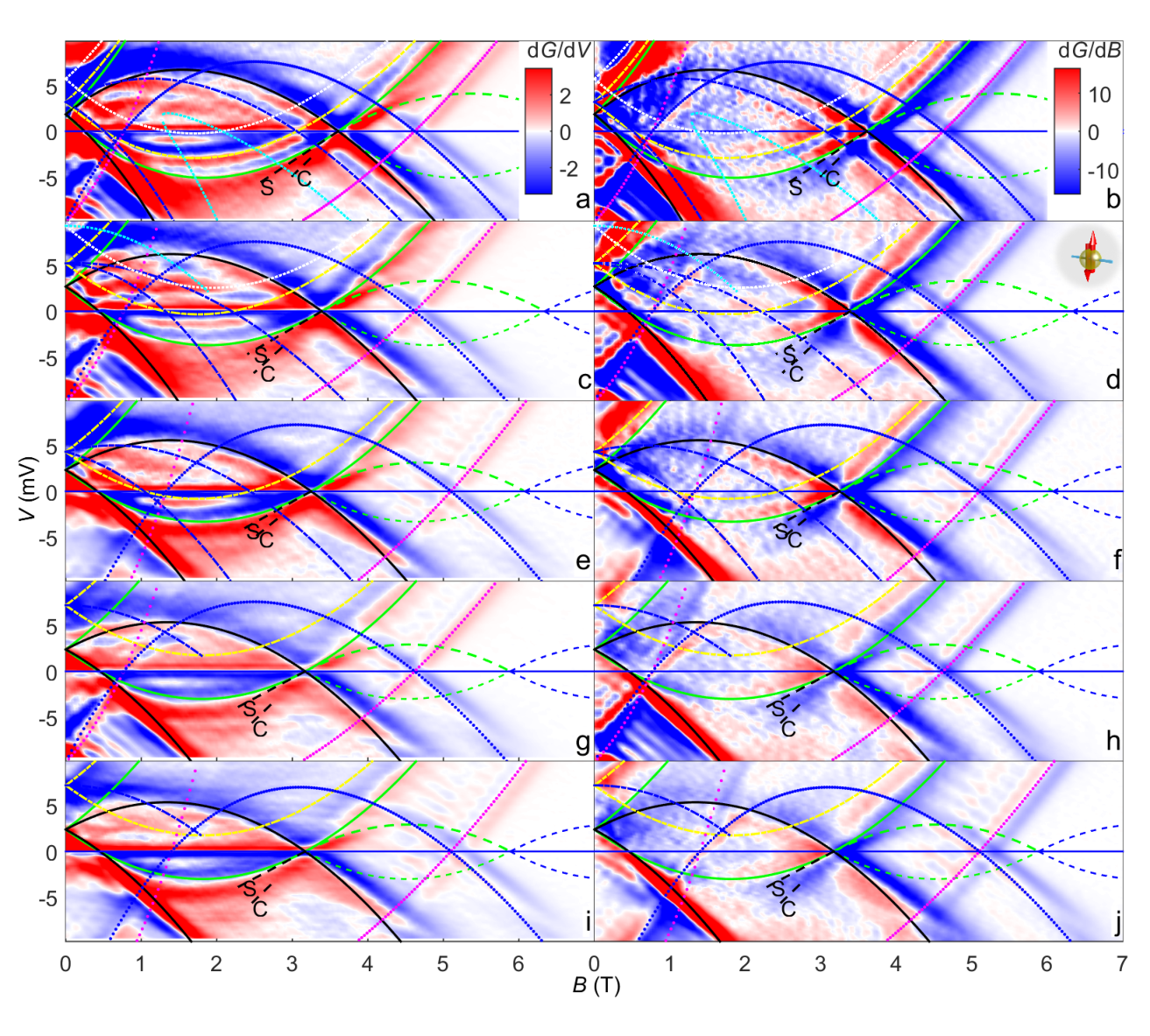
Now we extend the ranges of the voltage and magnetic field measuring the tunneling conductance across the double quantum well in Fig. 6 accessing a large portion of the 1D spectral function from below to and from to , see Fig. 8. There is an unavoidable ‘parasitic’ (‘p’) tunneling from narrow 2D regions (light blue strips in Fig. 6) that connect the wires to the injector constriction. This superimposes a set of parabolic 2D-2D dispersions on top of the 1D-2D signal, which are marked by magenta and blue dotted lines in Fig. 8.
Apart from the parasitic and the 2D dispersion signals, we observe only a single 1D parabola away from , marked by the solid green line in Fig. 8. It extends from the spin-excitation branch at low energy and the position of its minimum multiplied by the electronic charge gives the 1D chemical potential meV. The and crossings with the line , corresponding to momenta and , give the 1D Fermi momentum m-1. All other edges of the 1D spectral function are constructed by mirroring and translation of the hole part of the observable 1D dispersion, dashed green and blue lines in Fig. 8.

For positive voltages in the region just above the higher crossing point (, which corresponds to ) we observe a distinctive feature: the 1D peak broadens, instead of just continuing along the non-interacting parabola, with one boundary following the parabola () and the other bending around, analogous to the replica . This is visible in the conductance, but is most easily seen in the differentials, particularly (left column of Fig. 8). The broadening is observed at temperatures from 100 mK up to at least 1.5 K, and in samples with different wire designs (with or without air bridges) and lengths: in Fig. 9, is shown in detail for the broadened ‘replica’ region for the 10 m wires already presented (a–d), and for another sample with wires 18 m long (e, f). is plotted in Fig. 9b, d and f on cuts along the axis of the corresponding plots in the left column at various fields from to 4.8 T—between the ‘+’ and ‘’ symbols on each curve is a region of enhanced conductance characteristic of the replica .
Filling of the second 1D subband changes significantly the screening radius for the Coulomb interaction potential in the first 1D subband. This is manifested by a change of the ratio when the occupation of the second subband is changed by varying voltage of the finger gates in Figs. 8aceg, see Table 2. The ratio is a measure of interaction energy. Thus, the finger gates give a degree of experimental control over the interactions within our design of the 1D system. We use the maximum change of the ratio for different finger gate voltages to estimate the relative change of the interaction strength as obtaining a change of about .
It also has to be noted that the ‘replica’ is visible even when a second subband is present in the 1D wires, see Fig. 8a–f. In a and b it appears to go 25–30% higher in voltage than expected for a precise copy of the usual 1D parabola (even allowing for capacitive correction) due to a contribution of the second subband, which we do not analyse in detail here.
At even higher magnetic fields the line passes a ‘p’ parabola. Figs. 9a and c (and the corresponding cuts b and d) show the replica feature for two different positions of the ‘p’ parabolae using a gate above most of the ‘p’ region, showing that the replica feature is independent of the ‘p’ tunneling. The amplitude of the feature dies away rapidly, and beyond the ‘p’ parabolae, we have measured up to 8T with high sensitivity, but find no sign of any feature that can be distinguished from the decaying tails of the other features.
In the range of fields where the feature is observed its strength decreases as the field increases away from the crossing point analogously to the power-law for spinless fermions in Table 1. On general grounds it is natural to expect that divergence of the spectral weight of a b-mode toward an a-mode is a general feature, but there is no known method for performing a microscopic calculation in the spinful case. A similar feature should mark the mode (see Fig. 3 and Table 1) for negative voltages and for the magnetic field just below the crossing point , but it would be very difficult to resolve due to the overlaying spin and charge lines.

Making an analogy with the microscopic theory for spinless fermions in the first part of this paper, we estimate the ratio of signals around different spectral edges using the 1D Fermi wavelength, nm for our samples, as the short-range scale . The signal from the principal parabola, see Fig. 8b, gives the amplitude of the -mode as S. Then the amplitude of the signal from the second (third)-level excitations is predicted to be smaller by a factor of more than (), where the length of a wire is m. These values S (S) are at least two orders of magnitude smaller than the background and noise levels of our experiment S, which places an upper limit on the amplitude of any replica away from . Thus, our observations are consistent with the mode hierarchy picture for fermions.
In an effort to quantify the decay of the replica feature we have fitted the gradual background fall in conductance and the non-interacting 1D and 2D peaks (solid green and blue lines in Figs. 7–9) with a Gaussian and/or Lorentzian functions of , at each value of . The fitting parameters are then fitted to smooth functions in order to represent the general behaviour of the peaks as a function of . This idealised landscape is then subtracted from the data, see Fig. 10a, and the ‘replica’ is then fairly easily observed in the remaining conductance. A copy of a nearby region along the ‘p’ curve is then subtracted too, as an approximation to the rather diffuse signal arising from the main ‘p’ peak and smaller versions of it at slightly different densities. This also reduces errors in the peak and background fitting used in (a). We then plot the conductance along the expected parabola (dashed line in (a)) as a function of . This data is shown as circles in (c), where all the other contributions to the conductance along the same parabola are shown. Here, T and m-1. It is very hard to be sure that this procedure is reliable due to significant error bars imposed by contributions from the various other peaks, but it is clear that the replica feature dies away rapidly as a function of , and it is consistent with the law predicted for in Table 1 for . Though the overall prefactor is unknown theoretically in the spinful case, this singular power law may overcome the reduction factor close to .
IX Conclusions
In this work, we have shown that a hierarchy of modes emerges in systems of interacting fermions in one dimension at high energy controlled by the system length, in marked contrast to the well-known fermionic quasiparticles of a Fermi liquid and hydrodynamic modes of a Luttinger liquid at low energy.
We have obtained theoretically the dynamic response functions for a model of spinless fermions with short-range interactions using the exact diagonalisation methods of the Bethe ansatz for the spectrum and the form factors of the system. Analysing the spectral function in detail, we have found that the first-level (strongest) mode in long systems has a parabolic dispersion, like that of a renormalised free particle. The second-level excitations produce a singular power-law line shape for the first-level mode and different kinds of power-law behaviour at the spectral edges. Evaluating the form factor necessary for the dynamical structure factor we have shown that it has the same general form as the form factor of the spectral function, manifesting the same hierarchy of modes.
Using the same many-body matrix elements obtained microscopically, we have also calculated the local density of states. It provides a more convenient way to analyse how the hierarchy at high energy changes into the hydrodynamic modes of the Luttinger liquid at low energies. We have shown, via a full Bethe-ansatz calculation, that the LDOS is suppressed at the Fermi energy in a power-law fashion in full accord with the prediction of the Tomonaga-Luttinger model. Away from the Fermi point, where the Lorentz invariance of the linear dispersion is reduced to Galilean by the parabolicity of the spectrum, the LDOS is dominated by the first (leading) level of the hierarchy. We have demonstrated that the transition from one regime to another is a smooth cross-over.
We measure momentum-resolved tunnelling conductance in one-dimensional wires formed in the GaAs/AlGaAs double-well heterostructure by an array of finger gates. In this set-up we probe the spectral function of unpolarised electrons (spinful fermions) and find a pronounced spin-charge separation at low energy with a ratio of the spin and the charge velocities up to 1.8, which confirms that our system is in the strongly interacting regime. By varying the gate voltage that controls the width of our 1D wires, we demonstrate control of the interaction strength of about ; the deeper confining potential of the wires populates higher 1D subbands as well which in turn screens stronger Coulomb interactions in the principal 1D band reducing the interaction strength. In m-long wires we find a clear feature resembling the second-level excitations, which dies away rapidly at high momentum. A qualitative fit shows that the feature decays in a fashion that is consistent with the power-law prediction in this paper for spinless electrons.
Thus we have shown that the hierarchy is apparently a generic phenomenon at least for one- and two-point correlation functions of fermions without spin, and for a transport experiment for fermions with spin.
Acknowledgements.
We acknowledge financial support from the UK EPSRC through grant numbers EP/J01690X/1 and EP/J016888/1 and from the DFG though SFB/TRR 49. This research was supported in part by the National Science Foundation under Grant No. NSF PHY11-25915.References
- [1] P. Nozières, Theory of Interacting Fermi Systems (Addison-Wesley, 1997).
- [2] T. Giamarchi, Quantum physics in one dimension (Clarendon press 2003).
- [3] B. Roulet, J. Gavoret, and P. Nozières, Phys. Rev. 178, 1072 (1969).
- [4] P. Nozières, J. Gavoret, and B. Roulet, Phys. Rev. 178, 1084 (1969).
- [5] P. Nozières and C. T. de Dominicis, Phys. Rev. 178, 1097 (1969).
- [6] A. Imambekov, T. L. Schmidt, and L. I. Glazman, Rev. Mod. Phys. 84, 1253 (2012).
- [7] O. Tsyplyatyev, A. J. Schofield, Y. Jin, M. Moreno, W. K. Tan, C. J. B. Ford, J. P. Griffiths, I. Farrer, G. A. C. Jones, and D. A. Ritchie, Phys. Rev. Lett. 114, 196401 (2015).
- [8] N. A. Slavnov, Theor. Math. Phys. 79, 502 (1989).
- [9] O. Tsyplyatyev and A. J. Schofield, Phys. Rev. B 90, 014309 (2014).
- [10] G. Barak, H. Steinberg, L. N. Pfeiffer, K. W. West, L. Glazman, F. von Oppen, and A. Yacoby, Nature Physics 6, 489 (2010).
- [11] O. M. Auslaender, A. Yacoby, R. de Picciotto, K. W. Baldwin, L. N. Pfeiffer, and K. W. West, Science 295, 825 (2002).
- [12] Y. Jompol, C. J. B. Ford, J. P. Griffiths, I. Farrer, G. A. C. Jones, D. Anderson, D. A. Ritchie, T. W. Silk, A. J. Schofield, Science 325, 597 (2009).
- [13] V. E. Korepin, N. M. Bogoliubov, A. G. Izergin, Quantum inverse scattering methods and correlation functions (Cambridge University Press, 1993).
- [14] F.D.M. Haldane, Phys. Lett. A 81, 153 (1981).
- [15] J. von Delft and H. Schoeller, Ann. Phys. 7, 225 (1998).
- [16] A. A. Abrikosov, L. P. Gorkov, I. E. Dzyaloshinski, Methods of quantum field theory in statistical physics (Dover Publications, New York, 1975).
- [17] N. Kitanine, J.M. Maillet, V. Tetras, Nucl. Phys. B 554, 647 (1999).
- [18] N. Kitanine, J.M. Maillet, Nucl. Phys. B 567, 554 (2000).
- [19] P. Jordan and E. Wigner, Zeitschrift fur Physik 48, 631 (1928).
- [20] J.M. Maillet and J. Sanchez de Santos, Amer. Math. Soc. Transl. (2) 201, 137 (2000).
- [21] V. G. Drinfeld, Sov. Math. Dokl. 28, 667 (1983).
- [22] F. Gohmann and V. E. Korepin, J. Phys. A: Math. Gen. 33. 1199 (2000).
- [23] K. Motegi and K. Sakai, Nucl. Phys. B 793, 451 (2008).
- [24] M. Gaudin, B. M. McCoy, and T. T. Wu, Phys. Rev. D 23, 417 (1981).
- [25] J.-S. Caux and J. M. Maillet, Phys. Rev. Lett. 95, 077201 (2005).
- [26] J.-S. Caux, R. Hagemans, and J. M. Maillet, J. Stat. Mech. 2005, P09003 (2005).
- [27] J.-S. Caux, P. Calabrese, and N. Slavnov, J. Stat. Mech. 2007, P01008 (2007).
- [28] R. G. Pereira, J. Sirker, J.-S. Caux, R. Hagemans, J. M. Maillet, S. R. White, and I. Affleck, Phys. Rev. Lett. 96, 257202 (2006).
- [29] R. G. Pereira, S. R. White, and I. Affleck, Phys. Rev. B 79, 165113 (2009).
- [30] J. Links, H.-Q. Zhou, R. H. McKenzie, and M. D Gould, J. Phys. A: Math. Gen. 36, R63 (2003).
- [31] D. Biegel, M. Karbach, and G. Muller, Europhys. Lett. 59, 882 (2002).
- [32] D. Biegel, M. Karbach, and G. Muller, J. Phys. A: Math. Gen. 36, 5361 (2003).
- [33] J. Sato, M. Shiroishi, and M. Takahashi, J. Phys. Soc. Jpn. 73, 3008 (2004).
- [34] M. Pustilnik, M. Khodas, A. Kamenev, and L. I. Glazman, Phys. Rev. Lett. 96, 196405 (2006),
- [35] M. Pustilnik, M. Khodas, A. Kamenev, and L. I. Glazman, Phys. Rev. B 76, 155402 (2007).
- [36] A. Imambekov and L. I. Glazman, Phys. Rev. Lett. 102, 126405 (2009).
- [37] A. Imambekov and L. I. Glazman, Science 323, 228 (2009).
- [38] O. M. Auslaender, H. Steinberg, A. Yacoby, Y. Tserkovnyak, B. I. Halperin, K. W. Baldwin, L. N. Pfeiffer and K. W. West, Science 308, 88 (2005).
- [39] Y. Tserkovnyak, B. I. Halperin, O. M. Auslaender and A. Yacoby, Phys. Rev. B, 68, 125312 (2003).
- [40] M. Khodas, M. Pustilnik, A. Kamenev, and L. I. Glazman, Phys. Rev. Lett. 99, 110405 (2007).
- [41] R. G. Pereira, J. Sirker, J.-S. Caux, R. Hagemans, J. M. Maillet, S. R. White, and I. Affleck, J. Stat. Mech. 2007, P08022 (2007).
- [42] A. Imambekov and L. Glazman, Phys. Rev. Lett. 100, 206805 (2008).
- [43] A. Kamenev and L. Glazman, Phys. Rev. A 80, 011603 (2009).
- [44] T. Schmidt, A. Imambekov, and L. Glazman, Phys. Rev. Lett. 104, 116403 (2010).
- [45] T. Schmidt, A. Imambekov, and L. Glazman, Phys. Rev. B 82, 245104 (2010).
- [46] F. H. L. Essler, Phys. Rev. B 81, 205120 (2010).
- [47] O. Tsyplyatyev and A. J. Schofield, Phys. Rev. B 88, 115142 (2013).
- [48] A. Altland, C. H. W. Barnes, F. W. J. Hekking, A. J. Schofield, Phys. Rev. Lett. 83, 1203 (1999).
- [49] B. Kardynal, C. H. W. Barnes, E. H. Linfield, D. A. Ritchie, K. M. Brown, G. A. C. Jones, and M. Pepper, Phys. Rev. Lett. 76, 3802 (1996).
Appendix A Eigenvalue equation in the algebraic framework
The eigenvalue of the transfer matrix in Eq. (19) can be evaluated using the commutation relations in Eqs. (16,17). Let be a Bethe state in the algebraic representation of Eq. (21). The results of acting with and operators on the state are obtained by commuting these operators from left to right though the product of in Eq. (21) and then by using the their vacuum eigenvalues in Eq. (20).
Let us consider the case of and the operator first. Commuting once by means of Eq. (16) gives
| (70) |
Applying Eq. (16) the second time gives
| (71) | |||||
where the vacuum eigenvalue of , , was substituted explicitly. The second terms in the first and the second lines of the above equation have the same operator form but different scalar factors. Summation of the two scalar factor, using the explicit form of and from Eq. (12), yields
| (72) |
Thus the four terms can be rewritten as only three terms,
| (73) |
Extension of the same procedure for gives
| (74) |
Commuting of the operator is done in the same way using Eq. (17) and yields
| (75) |
Thus a Bethe state in Eq. (21) parametrised by an arbitrary set of is not an eigenstate of the transfer matrix since acting of the operator on such a state does not only result in multiplying by a scalar but also generates many different states: the second terms in Eq. (74) and in Eq. (75). However, the coefficients in front of each of these extra states can be made zero by a specific choice of ,
| (76) |
When a set of satisfies the system of equations above, the corresponding Bethe state is an eigenstate of the transfer matrix, , with the eigenvalue given by the first terms in Eq. (74) and in Eq. (75),
| (77) |
Eq. (76) is the set of Bethe equations in the algebraic representation, Eq. (22) of the main part of the text, and Eq. (77) gives the eigenvalue of the transfer matrix, Eq. (24) of the main part of the text.
Appendix B Calculation of averages of the local density operator
The calculation of the average of the local density operator is done in the same way as for the field operator in Subsection IVc. We start from the lattice model in Eq. (2) and the corresponding construction of the algebraic Bethe ansatz in Subsection IVa.
The local density operator can be represented in terms of and operators as[17, 18]
| (78) |
The action of the second factor in the above expression on an eigenstate just gives a phase factor – see an explanation after Eq. (31) – that we will ignore since we are interested in the modulus squared of this form factor. Then commuting the operator of the first factor in the equation above through all operators of the eigenstate – in the form in Eq. (21) – gives the result in Eq. (75).
The scalar product of Eq. (75), where the auxiliary parameter is set to , with another eigenstate gives
| (79) |
where is a Bethe state which is constructed from the eigenstate by replacing quasimomenta with . Note that the properties , where satisfy the Bethe equations and is an arbitrary set of quasimomenta,[17, 18] was used.
The scalar product in the first line in Eq. (79) is given by Eqs. (27, 28) where and are swapped. Substitution of in the same expressions for the scalar products in the second line of Eq. (79) yields
| (80) |
where all matrix elements of are
| (81) |
for
| (82) |
for .
After pulling a common factor out of the brackets in Eq. (79) and absorbing the -dependent prefactors in front of the determinants in the second line of Eq. (79) into the columns of the matrices under the determinants, the form factor in Eq. (79) reads as
| (83) |
Here the matrix elements of , which are obtain by multiplying by the corresponding scalars, are
| (84) |
for
| (85) |
for Note that for .
Finally, the summation over in Eq. (83) can be evaluated using a general matrix identity: where is obtained from the matrix by substituting column from matrix . After constructing the matrix out matrix elements from Eq. (85) and performing the summation over in Eq. (83), the form factor reads
| (86) |
where the matrix elements of are
| (87) | |||||
Now we evaluate the long wavelength limit for the result above. Applying the inversion mapping from the algebraic to the coordinate representation from Eq. (35) to the matrix elements in Eq. (87) and expanding the result up to the leading order we obtain,
| (88) |
Repeating the same procedure for the prefactor in Eq. (86) and pulling a common scalar factor out of the matrix elements under the determinant we obtain
| (89) |
where the matrix elements of are
| (90) |
and .
Evaluating the determinant we obtain
| (91) |
This formula can be proved by induction analogously to the proof of Eq. (43).