Oscillation in power spectrum of primordial gravitational wave as a signature of higher-order stringy corrections
Abstract
In low-energy effective string theory, corrections involve the coupling of the dilaton field to Gauss-Bonnet term. We assume that the dilaton potential is fine tuned so that the dilaton field may oscillate rapidly for a while around the minimum of its potential but the inflation background is not affected. By numerical method, we find that if the dilaton starts to oscillate at the time of about e-folds before the end of inflation, correction may bring unusual oscillations to the inflationary gravitational wave spectrum, which might be measurably imprinted in the CMB B-mode polarization.
I Introduction
In the recent years, high-precision CMB observations [1] confirmed the predictions of inflation. Meanwhile, the searching for the primordial tensor perturbations, i.e., the primordial gravitational waves (GWs) [2],[3], which may be imprinted in the CMB B-mode polarization spectrum [4],[5], has been still on road, e.g., [6]. The detection of primordial GWs would verify general relativity (GR) and strengthen our confidence in inflation. Inflation occurred in the early universe with higher scale. Thus, it could be expected that the primordial GWs might encode information of the UV-complete quantum gravity (e.g., [7]), for which the most promising candidate is string theory.
The effective action of string theory reduces to GR at low energy. However, it will acquire the higher-order curvature corrections with the expansion. In heterotic string theory, the leading-order correction is [8]
| (1) |
where is the Gauss-Bonnet (GB) term, is the string scale and is the dilaton field. In Type II string theory, it is , e.g., [9], see also Ref.[10] and references therein.
The effects of corrections are actually negligible at low energy . Thus the common expectation is that these characters of string theory can be hardly directly tested in laboratory experiments. However, inflation, which occurred in higher energy scale, is a natural laboratory for testing higher energy physics, since the corresponding physics might have an influence on the primordial perturbations produced during inflation. The model buildings of inflation in string theory has been widely investigated, e.g., [11] and [12],[13] for recent reviews.
The inflationary GWs is a powerful tool to probe the physics beyond GR, since it is only affected by the physics relevant to gravity, e.g., the change of the propagating speed of GWs [14]. Though the primordial scalar perturbation is affected also by the modified gravity, it is mainly affected by the dynamics of inflaton field itself, which will interfere the identifying of corresponding signatures. In Refs. [15],[16],[17],[18], the non-Gaussianities of inflationary GWs from modified gravity were studied. However, such non-Gaussianities are far below the sensitivity of on-road measurements. Comparatively, the power spectrum of primordial GWs is observationlly promising. Thus a significant asking is if corrections in string theory may leave measurable imprints in the CMB through their effects on the power spectrum of GWs.
Here, we assume that the dilaton potential is fine tuned so that the dilaton field may oscillate rapidly for a while around the minimum of its potential but the inflation background is not affected. By numerical method, we find that if the dilaton starts to oscillate at the time of about e-folds before the end of inflation, correction (1) can lead to the unusual oscillations in the power spectrum of primordial GWs. These oscillations may result in some obvious wiggles in the CMB B-mode polarization spectrum, which is well within the detection of the upcoming experiments. The intensity of the wiggles is determined by the string scale and the string coupling .
II The setup
The effective action of heterotic string may be [8],
| (2) |
where , and is dimensionless. The background is the inflation with , and the field driving inflation is given in (see, e.g., [13]), which we will not involve. The dimensionless scalar is the dilaton field. By variation with respect to metric, we obtain the modified Friedmann equations
| (3) |
| (4) |
where and are the energy density and pressure contributed by inflaton respectively. Here, for simplicity, we set as a ‘non-background’ field, i.e. spectator field, which means that it dose not dominate or affect the evolution of the background. This requires , and the contribution of from the GB term to must be also negligible, which put the constraint . In addition,
| (5) |
must be imposed, so that other higher-order corrections may be neglected, where is the string coupling.
The dilaton is massless in the weak coupling regime, i.e., and . However, in the moderately strong coupling regime, , the potential must exhibit some structure to make trapped at the minimum of the potential, so that the equivalence principle is preserved at late time [19]. Though the detail of the dilaton potential is still an issue in the study, it is generally thought that with a local valley can naturally arise due to some nonperturbative effects [20].
Inflation happens when inflaton dominates over other fields. We can see from Eq.(3) that it’s unlikely at the beginning of inflation, since the term with will dominate over the contribution from inflaton. Thus, it’s natural to assume that locates at the strong or moderately strong coupling regime with at the beginning of inflation, and runs towards the regime with until trapped by the valley of . In addition, we also require that the initial value of must also be negligible compared with the inflaton potential.
In this setup, the adiabatic scalar perturbation is contributed by inflaton, which is irrelevant with the ‘non-background’ field . We, following [21], may obtain the quadratic action of the GWs mode as follows
| (6) |
where satisfies and , is the conformal time, , a prime denotes the derivative with respect to , is the propagating speed of primordial GWs, and is regarded as effective Planck scale , and
| (7) |
where , which are consistent with the earlier results in Ref.[22][23]. Thus, although dose not dominate the background, due to its coupling to , it may affect the tensor perturbation, see also [17] for similar case but with nonminimal derivative coupling to . Here, the conditions of avoiding the ghost instability are and .
Here, if sits in the minimum of its potential or slow rolls, we have and , the primordial GWs spectrum will only acquire a small correction [24],[25], and its shape will not be altered essentially. However, before resting at the minimum of its potential, if , the dilaton field might rapidly roll down towards the minimum of its potential and oscillate around it, which will lead to a short-time but drastic variation of the propagating speed of GWs, see (7). We will show that it is this variation, if happened during inflation, that will naturally imprint the leading-order string correction (1) to the large-scale primordial GWs.
In the pre-big bang scenario, the corrections were applied to solve the singularity problem of the big bang model, which will also leave imprints in the primordial GWs [26],[27]. However, these imprints appear at small scales, and are not relevant to the CMB polarization, unless the pre-big bang phase is followed by an inflationary phase [28],[29], or see [30].
III The signature of higher-order string correction
The power spectrum of primordial GWs is calculated as follows. The Fourier series of is
| (8) |
where , the polarization tensors satisfy , , and , , the commutation relation for the annihilation and creation operators and is . Thus we have the equation of motion for as
| (9) |
where
| (10) |
Initially, the perturbations are deep inside the horizon, i.e., , the initial condition is . The power spectrum of GWs is
| (11) |
Here, since both and experience the short-time but drastic variations, analytical solution is difficult to obtain. We will first exhibit the numerical results, which help to clearly display the nontrivial feature of GWs spectrum induced by correction.
III.1 The numerical solution
To facilitate the numerically solving of the perturbation equation, we introduce the variable [31]. Using , the evolving equation of and Eq. (9) can be rewritten as
| (12) |
| (13) |
where the subscript ‘’ denotes , and and are given by Eqs. (7) and (10), respectively. The initial condition of Eq. (13) is written as
| (14) |
where the initial value of is set as unity. We assume, without loss of generality, that the background of slow-roll inflation is described by constant , so that the Hubble parameter may be written as , in which is constant.
As has been argued, in the moderately strong coupling regime , due to the non-perturbative effects, the potential must exhibit some structure to make trapped at the minimum of the potential. Initially, might deviate from the minimum of its potential. In (2), the dimension of is the square of mass and is dimensionless. In term of Ref. [20], both and are , in which is the volume of extra dimensions. Thus with (5) and , we have . Therefore, will rapidly roll down, and oscillate around the minimum of the potential before getting rest. As long as are fixed (note that is still reserved), the result is actually insensible to other details of .
Here, for the purpose of numerical simulation, we set the potential locally as , where . To not interrupt inflation, it’s convenient to parameterise the potential locally as
| (15) |
where has the dimension of the square of mass, is a dimensionless constant. The purpose of introducing is to guarantee that doesn’t affect the background evolution when is large enough, as we can see from Eq.(3) and (4). We will set , then the value of is smaller than , thus is negligible compared with . There is some finetunning in the shape of the potential. The shape of dilaton potential is actually still an issue in study, and it is generally thought that in heterotic string theory the potential with a local valley might arise due to some nonperturbative effects. What we mainly focused on is that how the primordial GWs spectrum will be affected, if there is such a potential.
Because both the contributions from the Gauss-Bonnet and the potential is to move towards smaller value, won’t be frozen if it located at initially, and we don’t need to create very fine-tuned initial conditions for 11 1 We plot with different initial value in Fig.7,. Below, we will set , and the initial value of as .
In Fig.1, we plot the evolutions of , and . The field rolls down along its potential, and gets rest at the minimum of the potential after oscillating around it, since the inflation rapidly dilutes its kinetic energy. This evolution induces the oscillations of and . The oscillation amplitude of is far larger than that of , since is dominated by while is by , and can hardly be large enough since . We can see that both and are always satisfied in the regime we are interested in, thus there is no ghost instability. Here, from the values of relevant parameters, we have , which satisfies the condition (5).
It might be concerned that whether the contribution of the spectator scalar field to the background evolution can be safely negligible. To verify this issue, we set the contribution of in Eq.(3) and (4) as
| (16) |
| (17) |
respectively. We plot and with respect to in Fig.2, using the same parameters used in Fig.1. We can see that the contributions from the terms relevant with are negligible compared with that of inflaton in the regime we are interested in.


In Fig.3, we plot the ratio of the power spectrum to for different , and , in which is that of standard inflation without correction. In all cases, unusual oscillations in are present, which is obviously a universal character attributed to the nontrivial behavior of and , or more intrinsically said, the string theory might manifest. Though the particle production during inflation may also significantly affect the power spectrum of GWs [32],[33], it only leads to a bumplike modification, which is entirely different from the behavior of the oscillation showed here.
In Fig.4, we plot the CMB lensed BB-mode power spectrum, compared with that of inflation without correction, in which , and both and are those of standard inflation. Here, we have assumed that the power spectrum of the scalar perturbation is not affected by the nontrivial behavior of the dilaton , and is still . In addition, we also assumed that after inflation the dilaton rests at the minimum of its potential so that GR is covered. Thus, the effect of varying at late time may be neglected, or see [34] [35]. When the dilaton field is fixed, the GB term will not affect the evolution of the background, since it is the generalised Euler density of four-dimensional spacetime, and thus is a topological invariant and does not contribute to the equations of motion.
There are generally a recombination peak at and a reionization bump at . Both are the imprints of the primordial GWs. The detection of the recombination peak will be a confirmation that inflation has ever occurred, while detecting the reionization bump at low- would help us to understand the physics of pre-inflationary universe, e.g.,[36]. When the comoving oscillating scale in GWs power spectrum is set at , for we may see obvious wiggles around the recombination peak, which may be tested by the upcoming polarization data.
III.2 The analytic estimate
The oscillations in are induced by correction, which naturally implies that the intensity of the oscillations is closely related to the value of the string scale . We have observed in Fig.3 that with larger , i.e., smaller energy scale of string , we got larger amplitude of the oscillation in the power spectrum. To acquire more insights on relevant physics, we will give an analytic estimate for it.
To not affect the background evolution, , and must be satisfied. Thus we have and . In addition, we have , so when rapidly rolls down and oscillates around the minimum of its potential, which corresponds to , in Eq. (12) dominates , i.e., . The second term in Eq. (12) is not negligible, which is responsible for making the oscillation stop rapidly. Thus our estimate is precise only for the first two or three oscillations. However, it is enough for us to grasp the physics behind the oscillating . When oscillates around , will acquire an oscillation with same frequency. The extreme values of the oscillating amplitude of can be estimated as
| (18) |
where is approximately replaced with . Therefore, for , we may have , which is required for the spectrum showing itself feature.
We assume that experiences an ideally steplike jump from to , and following Ref. [14] (see, also [37] for the scalar perturbation), we have
| (19) |
where
| (20) |
for , which oscillates between and , and is the wave number of the GWs mode crossing horizon when jumps, and .
Thus we approximately have
| (21) |
This reflects the effect of , which corresponds to , on the amplitude of oscillation in the power spectrum. In turn, we have
| (22) |
where and is dimensionless. This indicates that if the upcoming CMB B-mode polarization experiments would uncover wiggles in the B-mode power spectrum, it may offer important information about , the string coupling and the shape of the dilaton potential.

In Fig.5, we plot with respect to for different values of , in which for the heterotic string. To keep , we require . In addition, the result of Planck [1] showed the scalar perturbation amplitude , so (5) becomes for . In performing Fig.5, all above conditions are satisfied.
The power spectra plotted in Fig.3 indicates , and for the magenta dotted, green dashed and brown solid curves, respectively, which are consistent with Eq. (22) and Fig.5. Thus Eq. (22) actually works well for the first two or three oscillations. This provides a direct link between the oscillating amplitude in the primordial GWs spectrum and the string parameters, which is depicted in Fig.5.
In heterotic string theory, the spacetime is 10-dimensional. The leading term of the effective action is in the string frame, in which . After compactifying it on a Calabi-Yau manifold with volume , in four-dimension we have , e.g., [38]. Thus combining it with Fig.5, in which we see for , we have
| (23) |
for . This is consistent with the requirement of supergravity approximation, i.e., .
Here, for simplicity, we required that the background is not affected by the dilaton field. However, it is also possible that the dilaton field would affect the background at certain level. In that case, it is required to evaluate the effect of correction on the scalar perturbation spectrum. Additionally, the oscillation of primordial GWs power spectrum will also affect the auto-bispectrum of the tensor perturbations and the cross-bispectrum of the primordial perturbations, which will be studied in upcoming work.
IV Conclusion
The correction (1) can be regarded as high-order correction to GR. Due to some nonperturbative effects, the dilaton potential might show itself a local valley. We assume that the dilaton potential is fine tuned so that the dilaton field may oscillate rapidly for a while around this valley but the inflation background is not affected.
We numerically find that if the dilaton starts to oscillate at the time of about e-folds before the end of inflation, the correction (1) may bring unusual oscillations to the inflationary GWs spectrum, which might be measurably imprinted in the CMB B-mode polarization. We analytically show that the intensity of oscllating the is determined by the string scale and the string coupling .
We show that if , we might observe obvious wiggles around the recombination peak in the CMB B-mode power spectrum, which may be well within the detection of the current B-mode polarization experiments. This finding, if supported by observations, would yield significant insights into the gravity theory beyond GR. Conversely, a null result would place tight constraints on corresponding theory. Our work highlights the fact that high-precision CMB B-modes polarization experiments might offer us richer information on a UV-complete gravity theory than expected.
Acknowledgments
We thank Mingzhe Li, Jianxin Lu and Kaixi Feng for valuable discussions. This work is supported by NSFC, No. 11222546, and National Basic Research Program of China, No. 2010CB832804, and the Strategic Priority Research Program of Chinese Academy of Sciences, No. XDA04000000. We acknowledge the use of CAMB.
Appendix A The isocurvature perturbations from
The curvature perturbation is induced by inflaton, while the perturbation of the spectator field is the isocurvature perturbation. By perturbing with , we have
| (24) | |||||
Thus is instability-free. Actually, we have , since and , see Eq.(16), otherwise will dominate the background. Thus during inflation the curvature perturbation is hardly affected by the spectator scalar field . In addition, when perturbed, also contributes such as
| (25) |
which are higher-order and do not appear in the quadratic action of . This implies that as long as inflaton is canonical, is also instability-free.
However, after inflation the isocurvature perturbation from possibly converts to the curvature perturbation. In this Appendix, we will demonstrate that the isocurvature perturbation from is negligible.
We can set constant for an analytic estimate [39]. Then the solution can be given as
| (27) |
When , the power spectrum of is nearly scale-invariant. However, when , is imaginary. For convenience, we set . Using that , we have for . Thus the power spectrum of on superhorizon scales is given as
| (28) |
which is blue-tilted () with a strongly suppressed factor . Hence, the isocurvature perturbation from is negligible on large scale.
However, for the quartic potential we used, varies with time, Eq.(26) isn’t able to be solved analytically. But as long as , is strongly suppressed on the large scale. To demonstrate this speculation, we numerically solve Eq.(26) and plot in Fig.6 with the same parameters in Fig.1. We can see that the isocurvature perturbation from is negligible on large scale. Thus even if after inflation it can be converted to the curvature perturbation, its effect to the curvature perturbation from inflaton can be also safely neglected on the corresponding scale.

Appendix B The 3+1 decomposition of
To derive the perturbation action (6), we should do the decomposition of the Gauss-Bonnet term 22 2 This result was first obtained by Kaixi Feng. For more details, see Feng’s upcoming paper..
We follow the ADM metric
where is the lapse function, is the shift vector and is the spacial metric. It is useful to define the normal vector of 3-dimensional hypersurface and . Using the normalization , one have , which implies , and the 3-dimensional induced metric, which is orthogonal to the normal vector, i.e. , can be defined to be ,
Thus using the 3-dimensional variables, , and can be written as
| (39) | |||||
| (40) | |||||
| (41) |
where is the covariant derivative with respect to , is the Lie derivative in -direction, is the extrinsic curvature, and . Thus after defining , we have
| (42) | |||||
Till now, has been decomposed and presented with only , and -related variables. Then, after tedious derivation, the action (6) of the tensor perturbation can be obtained by taking , where satisfies and .
Appendix C The evolution of with different initial value
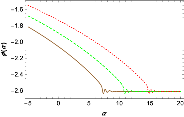
References
- [1] P. A. R. Ade et al. [Planck Collaboration], arXiv:1502.02114 [astro-ph.CO].
- [2] A. A. Starobinsky, JETP Lett. 30, 682 (1979).
- [3] V. A. Rubakov, M. V. Sazhin and A. V. Veryaskin, Phys. Lett. B115, 189 (1982).
- [4] M. Kamionkowski, A. Kosowsky and A. Stebbins, Phys. Rev. Lett. 78, 2058 (1997) [astro-ph/9609132].
- [5] U. Seljak and M. Zaldarriaga, Phys. Rev. Lett. 78, 2054 (1997) [astro-ph/9609169].
- [6] P. A. R. Ade et al. [BICEP2 and Planck Collaborations], Phys. Rev. Lett. 114, 10, 101301 (2015) [arXiv:1502.00612 [astro-ph.CO]].
- [7] E. Silverstein, arXiv:1311.2312 [hep-th].
- [8] R. R. Metsaev and A. A. Tseytlin, Nucl. Phys. B 293, 385 (1987).
- [9] D. J. Gross and E. Witten, Nucl. Phys. B 277, 1 (1986).
- [10] D. Ciupke, J. Louis and A. Westphal, arXiv:1505.03092 [hep-th].
- [11] K. i. Maeda and N. Ohta, Phys. Lett. B 597, 400 (2004) doi:10.1016/j.physletb.2004.07.038 [hep-th/0405205]; K. i. Maeda and N. Ohta, Phys. Rev. D 71, 063520 (2005) doi:10.1103/PhysRevD.71.063520 [hep-th/0411093]; K. Akune, K. i. Maeda and N. Ohta, Phys. Rev. D 73, 103506 (2006) doi:10.1103/PhysRevD.73.103506 [hep-th/0602242]; Z. K. Guo, N. Ohta and S. Tsujikawa, Phys. Rev. D 75, 023520 (2007) doi:10.1103/PhysRevD.75.023520 [hep-th/0610336].
- [12] C. P. Burgess, M. Cicoli and F. Quevedo, JCAP 1311, 003 (2013) [arXiv:1306.3512 [hep-th]].
- [13] D. Baumann and L. McAllister, arXiv:1404.2601 [hep-th].
- [14] Y. Cai, Y. T. Wang and Y. S. Piao, Phys. Rev. D 91, 10, 103001 (2015) [arXiv:1501.06345 [astro-ph.CO]].
- [15] J. M. Maldacena and G. L. Pimentel, JHEP 1109, 045 (2011) [arXiv:1104.2846 [hep-th]].
- [16] X. Gao, T. Kobayashi, M. Yamaguchi and J. Yokoyama, Phys. Rev. Lett. 107, 211301 (2011) [arXiv:1108.3513 [astro-ph.CO]].
- [17] K. Feng, T. Qiu and Y. S. Piao, Phys. Lett. B 729, 99 (2014) [arXiv:1307.7864 [hep-th]];
- [18] K. Feng and T. Qiu, Phys. Rev. D 90, 12, 123508 (2014) [arXiv:1409.2949 [hep-th]].
- [19] T. Damour, F. Piazza and G. Veneziano, Phys. Rev. Lett. 89, 081601 (2002) [gr-qc/0204094].
- [20] E. Silverstein, hep-th/0405068.
- [21] J. M. Maldacena, JHEP 0305, 013 (2003) [astro-ph/0210603].
- [22] S. Kawai, M. a. Sakagami and J. Soda, Phys. Lett. B 437, 284 (1998) [gr-qc/9802033].
- [23] C. Cartier, J. c. Hwang and E. J. Copeland, Phys. Rev. D 64, 103504 (2001) [astro-ph/0106197].
- [24] P. X. Jiang, J. W. Hu and Z. K. Guo, Phys. Rev. D 88, 123508 (2013) [arXiv:1310.5579 [hep-th]].
- [25] A. De Felice and S. Tsujikawa, Phys. Rev. D 91, 10, 103506 (2015) [arXiv:1411.0736 [hep-th]].
- [26] M. Gasperini, Phys. Rev. D 56, 4815 (1997) [gr-qc/9704045].
- [27] C. Cartier, E. J. Copeland and M. Gasperini, Nucl. Phys. B 607, 406 (2001) [gr-qc/0101019].
- [28] Y. S. Piao, B. Feng and X. M. Zhang, Phys. Rev. D 69, 103520 (2004) [hep-th/0310206].
- [29] Z. G. Liu, Z. K. Guo and Y. S. Piao, Phys. Rev. D 88, 063539 (2013) [arXiv:1304.6527].
- [30] M. Satoh, S. Kanno and J. Soda, Phys. Rev. D 77, 023526 (2008) [arXiv:0706.3585 [astro-ph]].
- [31] J. A. Adams, B. Cresswell and R. Easther, Phys. Rev. D 64, 123514 (2001) [astro-ph/0102236].
- [32] J. L. Cook, and L. Sorbo, Phys. Rev. D 85, 023534 (2012) [arXiv:1109.0022 [astro-ph.CO]].
- [33] L. Senatore, E. Silverstein and M. Zaldarriaga, JCAP 1408, 016 (2014) [arXiv:1109.0542 [hep-th]].
- [34] L. Amendola, G. Ballesteros and V. Pettorino, Phys. Rev. D 90, 4, 043009 (2014) [arXiv:1405.7004 [astro-ph.CO]].
- [35] M. Raveri, C. Baccigalupi, A. Silvestri and S. Y. Zhou, Phys. Rev. D 91, no. 6, 061501 (2015) [arXiv:1405.7974 [astro-ph.CO]].
- [36] Y. Cai, Y. T. Wang and Y. S. Piao, Phys. Rev. D 92, 2, 023518 (2015) [arXiv:1501.01730 [astro-ph.CO]].
- [37] M. Nakashima, R. Saito, Y. i. Takamizu and J. Yokoyama, Prog. Theor. Phys. 125, 1035 (2011) [arXiv:1009.4394 [astro-ph.CO]].
- [38] K. Becker, M. Becker and J. H. Schwarz, ¡°String Theory and M-Theory,¡± Cambridge Univ. Press, 2007.
- [39] A. Riotto, hep-ph/0210162.