Localization and spin transport in honeycomb structures with spin-orbit coupling
Abstract
Transfer-matrix methods are used for a tight-binding description of electron transport in graphene-like geometries, in the presence of spin-orbit couplings. Application of finite-size scaling and phenomenological renormalization techniques shows that, for strong enough spin-orbit interactions and increasing on-site disorder, this system undergoes a metal-insulator transition characterized by the exponents , . We show how one can extract information regarding spin polarization decay with distance from an injection edge, from the evolution of wave-function amplitudes in the transfer-matrix approach. For (relatively weak) spin-orbit coupling intensity , we obtain that the characteristic length for spin-polarization decay behaves as .
pacs
72.15.Rn, 72.25.-b,72.80.VpI Introduction
In this paper we consider electronic transport in two-dimensional (2D) honeycombe-lattice structures with spin-orbit (SO) interactions. While single-parameter scaling predicts that noninteracting electron states in 2D are generally localized by disorder [1], it is known that in this marginal dimension the enhancement of forward scattering provided by SO effects can partially offset disorder-induced quantum interference, thus giving rise to a conducting phase [2, 3, 4]. Motivation for considering a honeycomb geometry is provided mostly by recent progress in experimental synthesis, and theoretical understanding, of graphene [5, 6, 7]. It should be noted that some of carbon’s cousin elements in group IVB have been predicted and, to varying degrees of success, shown to crystallize in a similar honeycomb arrangement, giving rise respectively to silicene [8] and germanene [9]. Stable honeycomb structures have also been found for boron nitride (h-BN) [10] as well as SiO2 (silicatene) [11] and other elements or compounds. The ideas and methods exhibited in what follows are, in principle, applicable to any of the above. However, where comparison of our results to experimental data is pertinent we generally restrict ourselves to graphene, as this is so far the best-understood member of the ensemble.
Our purpose here is twofold: (i) to investigate location and universality properties of the second-order metal-insulator found in these systems, for strong SO coupling, with increasing on-site disorder; and (ii) to examine the spatial evolution of the polarization of an initially fully spin-polarized current, injected into one such hexagonal-lattice system with SO couplings.
Section II below recalls selected existing results, as well as some technical aspects of the transfer-matrix (TM) method used in our calculations. In Sec. III we discuss the metal-insulator transition. In Sec. IV we show how one can extract information on the evolving state of polarization of an injected electron beam, from the analysis of wavefunction amplitudes generated via the TM method. In Sec. V we provide a global analysis of our results; finally, concluding remarks are made.
II Theory
The model one-electron Hamiltonian for this problem can be written as
| (1) |
where , are creation and annihilation operators for a particle with spin eigenvalues at site , and the self-energies are, in general, independently-distributed random variables; denotes the spin-dependent hopping matrix between pairs of nearest-neighbor sites , whose elements must be consistent with the symplectic symmetry of SO interactions.
Although modeling SO coupling in real systems usually relies on including e.g. orbitals, with their corresponding degeneracies, in Eq. (1) we resort to the customary description via an effective Hamiltonian with a single (like) orbital per site; for a pedagogically clear explanation of how this approach works from first principles, see e.g. the Appendix of Ref. 4. Since we shall not attempt detailed numerical comparisons to experimental data, such formulation seems adequate for our purposes.
In the effective-Hamiltonian context, there is some leeway as the specific form of the hopping term is concerned, depending on whether one is specifically considering Rashba- or Dresselhaus- like couplings [4, 12], or the focus is simply on the basic properties of systems in the symplectic universality class [13, 14, 15]. One constraint is that it must incorporate the basic symmetries of SO coupling, which have close connections with quaternion algebra [16, 17].
Here we use the implementation of Refs. 13, 14, namely:
| (2) |
where is the identity matrix, are the Pauli matrices, and gives the intensity of the SO coupling; below we consider the (real) as either uniform ( on all bonds) or randomly (uniformly) distributed in . Thus all energies will be written in units of the nearest-neighbor hopping.
Similarly the will either be constant, site-independent, or taken from a random uniform distribution in .
The form Eq. (2) for the hopping term does not exhibit the explicit multiplicative coupling between momentum and spin degrees of freedom, characteristic of Rashba-like Hamiltonians [4, 12]. A similarly-decoupled effective Hamiltonian can be derived from first principles for carbon nanotubes, see Eqs. (3.15), (3.16) of Ref. 18. In two dimensions one should not expect significant discrepancies between results from either type of approach, as long as one is treating systems without lateral confinement.
We apply the TM approach specific to tight-binding Hamiltonians like Eq. (1) [19, 20, 21] to finite-width strips of the honeycomb lattice, with sites across. Adaptation from the more usual square-lattice geometry is straightforward, closely following the lines used for the TM description of localized (e.g., Ising and Potts) spin systems [22, 23, 24, 25]. Two distinct orientations are possible [25, 26], with the TM proceeding either (a) perpendicularly [22] or (b) parallel to one lattice direction [23]. Case (a) corresponds to a "brick" lattice, i.e., a square lattice with vertical bonds alternately missing.
In the terminology of quasi one-dimensional carbon nanotubes (CNT) and nanoribbons (CNR) [5], a narrow strip with periodic boundary conditions across in geometry (a) would be topologically equivalent to an armchair CNT, while one in geometry (b) would correspond to a zigzag CNT. Conversely, free boundary conditions parallel to the TM’s direction of advance give: zigzag CNR in (a), armchair CNR in (b).
Detailed consideration shows that implementation of the TM scheme of Ref. 19 in geometry (b) involves a number of cumbersome intermediate operations [ mostly matrix inversions, see Eqs. (8)--(16) of Ref. 26 ]. In what follows we always make use of geometry (a), for simplicity.
We briefly recall selected aspects of the TM formulation introduced in Ref. 19, and of its adaptation for a honeycomb geometry with SO couplings.
Consider a strip of the square lattice, cut along one of the coordinate directions. For the orthogonal universality class with site disorder, denoting by the successive columns, and the respective positions of sites within each column of a strip, the recursion relation for an electronic wave function at energy is given in terms of its local amplitudes (which can all be assumed real), , and tight-binding orbitals , as:
| (3) |
where is the identity matrix, the energy dependence has been omitted for clarity, and (invoking periodic boundary conditions across the strip),
| (4) |
For a honeycomb lattice in the "brick" geometry, the changes to are [22, 23, 24, 25]: (i) the off-diagonal elements are of the form , reflecting the alternately missing vertical bonds; and (ii) an elementary step consists of applying the TM twice, in order to restore periodicity.
The introduction of SO couplings along the bonds, see Eqs. (1), (2), means that the are now spinors, written on the basis of the eigenvectors of as:
| (5) |
where the , are complex. The matrices and the subdiagonal of Eq. (3) are now , while the diagonal terms of are doubly degenerate, and the non-zero off-diagonal ones are replaced either by the (bond-dependent) negative of matrix of Eq. (2) or that of its hermitean adjoint , depending on whether they are supra- or sub-diagonal [27]. The negative unitary elements of the (now ) supradiagonal identity matrix of Eq. (3) are replaced by the bond-dependent negative of .
III Metal-Insulator Transition
III.1 Introduction
To make contact with previous work on the square lattice [13, 14, 15], we initially considered systems without site randomness, i.e., all , and two versions of SO coupling: (i) uniform with , in Eq. (1), (ii) random, with (as in Ref. 14) and , , uniformly distributed in .
In case (i), analysis of the resulting dispersion relation shows that the allowed states occupy a band with the same structure as that for a system with but, analogously to the square-lattice systems with uniform SO term of Ref. 14, in the range .
For case (ii) the corresponding density of electronic states (DOS) can be evaluated by making use of eigenvalue-counting theorems [28, 29, 30]. Our implementation takes advantage of the sparse nature of the Hamiltonian matrix written on the site basis, and resorts to Gaussian elimination algorithms on strip-like geometries (with periodic boundary conditions across), closely following the steps described in Refs. 31, 32, 33.
Since is calculated from the finite difference between successive values of integrated DOS up to adjacent energies and [31, 32, 33], the bin size has to be optimized in order to reduce oscillations in the numerical results while still capturing relevant structural details of the DOS. We generally took strip-like systems with sites across, and length , for which proved to be a reasonable choice. For cases such as (ii) where quenched randomness can play a role in inducing further fluctuations, we saw that for the system sizes used, the self-averaging provided by having a large(ish) number of local disorder realizations was enough to render such effects relatively unimportant.
We numerically evaluated , for both (i) [ as an independent check of the soundness of our algorithms ] and (ii). Results are shown in Fig. 1. For (i) we used , which ensures that equals of case (ii), where angular brackets stand for ensemble average.
One sees that the resulting bands indeed have the same width, although the shape of tails at the edges differs. As expected, these are rather abrupt in (i) and smoother in (ii), in line with the probabilistic character of the latter’s coupling distribution. Furthermore, while the band in case (i) keeps all qualitative features of the system, including the zero at , these are lost in case (ii); for example, the shallow minimum at the origin corresponds to .

Note that the effective strength of intrinsic SO coupling in graphene is estimated to be eV [34], of order of the nearest-neighbor hopping eV [5]. The values used in this Section are for illustration only, and not intended to reflect the actual properties of pure graphene. We return to this point in Sec. V below.
III.2 Phenomenological renormalization
Here the SO coupling is represented as in model (ii) of Sec. III.1, with (fixed). We now introduce site randomness, i.e. and zero otherwise, and allow the respective distribution width to vary.
Following standard procedures [19] we considered , at the Dirac point of the unperturbed Hamiltonian, and iterated the TM on strips of width sites and length with periodic boundary conditions across. The characteristic Lyapunov exponents were extracted [20, 21], with the longest localization length being given by the inverse of the smallest of those. According to finite-size scaling and the phenomenological renormalization ansatz, we plotted the scaled localization lengths against varying , looking for the mutual intersection of the curves corresponding to different strip widths which gives the location of the critical point of the metal-insulator transition.
We took , 12, 14, 16, 24, 32, and 48, with . The results are shown in Fig. 2.

It is known that nonlinearity of scaling fields and/or irrelevant variables [35] can cause sizable distortions in the estimates of critical quantities at Anderson localization transitions. Efficient procedures have been devised to correct for effects of this sort [15, 36, 37]. We noted that if only strip widths were used, corrections to scaling due to irrelevant fields (usually dealt with by methods explained in Refs. 36, 37) were of little import. Thus we concentrated on accounting for nonlinearities [15].
Following the lines of Ref. 15 [ see especially their Eqs. (6)--(11) ], we define as the disorder distribution width at criticality, and with , we assume that:
| (6) |
where is a smooth function of and which goes to zero at criticality. At fixed , one then considers a truncated Taylor expansion of in terms of :
| (7) |
Nonlinearities in the argument of are thus taken into account with . Plugging this back into Eq. (6) one gets another truncated Taylor series near criticality:
| (8) |
where . One can either set in Eq. (7), or in Eq. (8) without loss of generality. It is expected that by using the logarithm in Eq. (6), the smoothness assumption underlying the Taylor expansions will be fulfilled with fewer terms than if the themselves were considered.
Fig. 3 shows the best-fitting scaling plot of the data of Fig. 2, for which we took , . Numerical values are given in Table 1.

The adjusted is in very good agreement with of Ref. 15 which is, to our knowledge, the most accurate result to date . Earlier work gave less accurate estimates, mostly in the range [ see Table 1 of Ref. 38 ].
For comparison of with results pertaining to the square lattice, one must recall the geometric correction factors of the honeycomb lattice [22, 23, 24, 25]. This means that, in order to produce an estimate of the decay-of-correlations exponent given by conformal invariance [35], the raw TM result for must be multiplied by a factor of . We thus obtain [ so ] which compares rather well with of Ref. 15. We note that the critical-amplitude results of Ref. 39 do not compare directly with ours because those authors study the scaling behavior of the typical localization length. As is known, this quantity is given by the zeroth moment of the correlation-function probability distribution [40], whereas here we deal with average quantities, i.e. ones related to the corresponding first-order moment.
IV Spin relaxation
In studies of spintronics in semiconductors [41, 42] the spin coherence length is one of the quantities of interest. Here we consider the decay of spin polarization in electronic transport in quasi one-dimensional geometries, in the presence of SO couplings. The subject is usually approached via Green’s function techniques [12]. We show that this problem can be investigated by considering the evolution of wavefunction amplitudes in the TM context [43, 44].
Usual TM treatments focus on extracting the spectrum of characteristic Lyapunov exponents, which demands repeated iteration along columns, with frequent orthogonalization to avoid contamination [19, 20, 21]. However, one sees that the recursion relation synthesized in Eq. (3) contains information on how the electron wavefunction evolves, starting from specified initial conditions. In presence of SO couplings the off-diagonal hopping matrix elements induce spin flips, thus affecting spin polarization along the system’s length.
Assume that a fully spin-polarized electron beam is injected into the system, i.e., , , . One can extract information about the beam’s polarization state lattice spacings down the strip by iterating Eq. (3) times and examining the resulting coefficients , . In this case the beam polarization at column is given by:
| (9) |
The initial conditions just mentioned can be viewed as representing an ideal lead, i.e., one without SO interaction, from which the beam is injected into the strip. Although, for a complete description one would need to take into account reflection at the injecting boundary (as well as at the strip’s end, presumably linked to a second ideal lead), these features do not influence the calculated polarization decay length, as this quantity is computed from ratios of (sums of squared) amplitudes each taken at a fixed position [12].
We evaluate spin polarization profiles on systems with periodic boundary conditions across, i.e., topologically equivalent to CNTs; we keep , fixed, as this corresponds to the Fermi energy which is the relevant level for transport phenomena. The SO couplings are again represented by model (ii) of Sec. III.1, although the overall amplitude will be allowed to vary. Our results are averages over typically independent samples. For each of these we generate random sets of the , , as well as the . Thus we are sampling over the ensemble of steady-flow configurations.
We consider the simplest case with no site randomness, i.e., all in Eq. (1). This removes one (finite) length scale from the problem, as one would have the [ site ] disorder-associated mean free path .
Fig. 4 shows that spin polarization settles into exponential decay against position along the nanotube’s axis, after a short transient region of steeper variation. The characteristic decay lengths are found by adjusting the appropriate sections of numerical data to a pure exponential-decay form.
For fixed , we found a slight dependence of on , which is strongest for small . As increases, saturation becomes evident and it is possible to estimate with good accuracy by using data for up to (see the inset to Fig. 5).

The main diagram in Fig. 5 shows that, to a very good extent, the relationship holds for the range . This is in line with the findings of Ref. 12 for quantum wires with nonzero on-site disorder and Rashba-like SO coupling. Such inverse-square dependence of on is thus likely to be a universal property for electronic transport in two-dimensional systems with SO effects.
Next, we introduce quenched impurities with SO interaction onto an otherwise pure system, i.e. one in which such interaction is generally absent. This amounts to a simplified representation of pure graphene (where, as recalled in Sec. III.1, SO coupling is very weak) doped with suitable impurities.
Many experimental and theoretical studies deal with impurities on CNRs, where edge effects play an important role in the energetics of favored defect locations . By considering only nanotube geometries, here we need not account for this sort of positional preference inhomogeneity. Furthermore, we restrict ourselves to so-called hole defects, i.e. adatoms which sit over the center of a hexagon [45].
Denoting by the fraction of randomly chosen hexagons which have an impurity atop their center, we assume that hopping along all six bonds which make such a hexagon is characterized by SO couplings as given in Eq. (2), with the , , randomly distributed as in case (ii) of Sec. III.1. We take as in Sec. III, which makes the adatom’s average SO interaction about as strong as the hopping term of pristine graphene.
We consider only and neglect effects due to adjacent impurities, which should be a reasonable approximation in this concentration range.
In Fig. 6 it can be seen that for the relaxation length is very close to that for a system with SO coupling on all bonds, and . For relatively short distances from the injection edge the initial decay rate is found to be distinctly higher for the latter case than for the former, as highlighted in the inset of Fig. 6. We refrain from ascribing much significance to this difference since we do not expect our approach to give an accurate description of such short-range effects. So, concerning the region farther than some lattice spacings from the origin, the effect on (asymptotic) spin polarization decay of of bonds with SO coupling is similar to that of all bonds having .

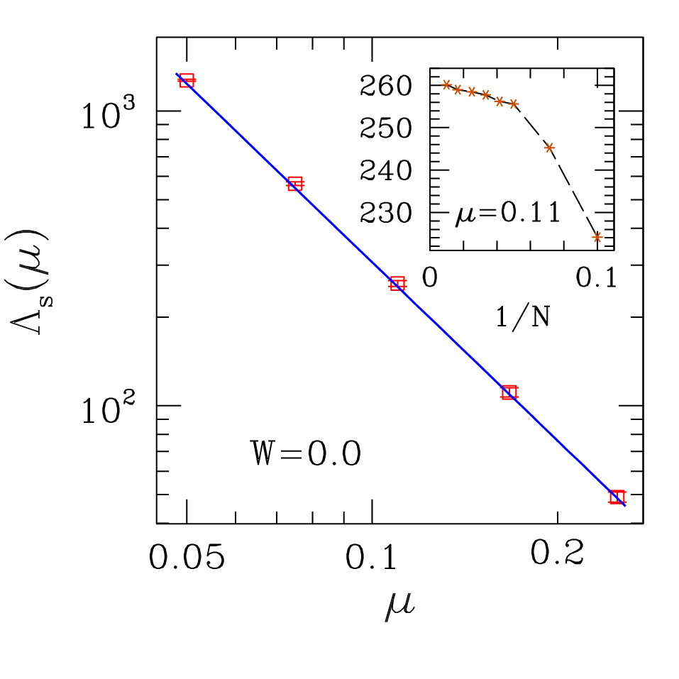
We checked the dependence of on and . For fixed we took , , , and which gave a rather good fit to a dependence with ; then for fixed we additionally made , , and . In this case one gets with . If one instead assumes that , found for smaller and systems with SO couplings on all bonds (see Fig. 5), still applies here, one gets:
| (10) |
where the large scatter in the estimate of reflects the aforementioned poor quality of the fits of behavior against varying . Nevertheless, Eq. (10) can be a rough-and-ready guide to estimate the relaxation length for values of and closer to physically realizable experiments than those used here.
V Discussion and Conclusions
We have studied model tight-binding Hamiltonians for the description of electron transport in graphene-like geometries, in the presence of SO couplings. Our main interest is in the behavior of very large sheet-like samples, although in the quasi-one dimensional context of the TM methods applied here, the use of periodic boundary conditions across makes our systems topologically akin to CNTs. For the latter type of system, especially in the limit of very narrow nanotubes, a more realistic description should probably incorporate curvature effects, as done in Ref. 18.
The energy unit used here equals the nearest-neighbor hopping parameter in pristine graphene, thus translating into eV [5]. The intrinsic SO coupling in graphene is estimated as eV [34]; weakly-hydrogenated samples have been reported as giving a colossal enhancement on this by three orders of magnitude [46]. The latter value would then correspond to , similar to the low end of the range investigated in Sec. IV, for systems with SO couplings on all bonds. On the other hand, we used , both in Sec. III and for impurity adatoms in Sec. IV, partly for comparison with extant work [13, 14, 15], and also in order to produce well-defined numerical results amenable to unequivocal interpretation.
In Sec. III we showed that for strong SO interactions a second-order metal-insulator transition takes place, which is in the same universality class as that found for square-lattice systems [4, 13, 14, 15]. Note that the energy used in our calculations corresponds to the Dirac point of pure graphene, at which (contrary to the square-lattice case) the tight-binding DOS vanishes identically. Although in real graphene a (quantized) non-zero minimum conductivity has been found at the Dirac point [47], the effect seen in our results is unrelated to this, being of a larger order of magnitude (the metallic phase extends up to site disorder of strength ). In fact, as can be seen in Figure 1, the random SO couplings used in the model investigated in Sec. III.2 account for the significant departure from zero of the DOS close to . So, it is the latter feature which sets the stage for the relative robustness of the conducting phase in our model. The above remark should apply also to the case of structures mentioned in Sec. I, such as boron nitride [10] or silicatene [11], which are wide gap insulators. Indeed, it is expected [48] that in general the introduction of randomness will be accompanied by the appearance of states outside the pure-system bands, in particular within the gap. Whether that will be enough to give rise to a conducting phase should depend on quantitative details of the disordered potential.
In Sec. IV we showed how one can extract information regarding spin polarization decay with distance from an injection edge, from the evolution of wave-function amplitudes in a TM context. We illustrated the pertinent ideas in the simple context of a nanotube-like geometry, with no on-site disorder, and investigated the dependence of the spin relaxation length on SO coupling strength . For small , closer to physically realizable values, we found the dependence which seems to be a universal relationship for two- (or quasi-one) dimensional systems with SO interactions [12]. For SO couplings acting only on impurity sites, randomly distributed with low concentration , we found numerically , in line with elementary probabilistic considerations.
It must be noted that modeling SO coupling via Eq. (2) with the , randomly distributed in gives an effect which is, on average, isotropic in spin space. So this formulation is not suitable, e.g., for a realistic discussion of precession effects.
Prospects for further application of the ideas presented in Sec. IV would include taking site disorder into account, as well as studying CNR geometries. For the latter, inhomogeneities in local current density in the transverse direction to average flow would be directly accessible.
Acknowledgements.
The author thanks the Brazilian agencies CNPq (Grant No. 303891/2013-0), and FAPERJ (Grants Nos. E-26/102.760/2012, E-26/110.734/2012, and E-26/102.348/2013) for financial support.References
- [1] E. Abrahams, P. W. Anderson, D. C. Licciardello, and T. V. Ramakrishnan, Phys. Rev. Lett. 42, 673 (1979).
- [2] S. Hikami, A. I. Larkin, and Y. Nagaoka, Prog. Theor. Phys. 63, 707 (1980).
- [3] G. Bergmann, Phys. Rep. 107, 1 (1984).
- [4] T. Ando, Phys. Rev. B40, 5325 (1989).
- [5] J-C. Charlier, X. Blase, and S. Roche, Rev. Mod. Phys. 79, 677 (2007); A. H. Castro Neto, F. Guinea, N. M. R. Peres, K. S. Novoselov, and A. K. Geim, ibid. 81, 109 (2009).
- [6] N. M. R. Peres, J. Phys. Condens. Matter 21, 323201 (2009).
- [7] E. R. Mucciolo and C. H. Lewenkopf, J. Phys. Condens. Matter 22, 273201 (2010).
- [8] A. Kara, H. Enriquez, A.P. Seitsonen, L.C. Lew Yan Voon, S. Vizzini, B. Aufray, and H. Oughaddou, Surf. Sci. Reports 67, 1 (2012).
- [9] A. Acun, L. Zhang, P. Bampoulis, M. Farmanbar, A. van Houselt, A. N. Rudenko, M. Lingenfelder, G Brocks, B.Poelsema, M. I. Katsnelson, and H. J. W. Zandvliet, J. Phys. Condens. Matter 27, 443002 (2015).
- [10] K.S. Novoselov, D. Jiang, F. Schedin, T.J. Booth, V.V. Khotkevich, S. V. Morozov, and A. K. Geim, Proc. Natl. Acad. Sci. USA 102, 10451 (2005).
- [11] V. O. Özçelik, S. Cahangirov, and S. Ciraci, Phys. Rev. Lett. 112, 246803 (2014).
- [12] T. Kaneko, M. Koshino, and T. Ando, Phys. Rev. B78, 245303 (2008).
- [13] S. N. Evangelou and T. Ziman, J. Phys. C 20, L235 (1987).
- [14] S. N. Evangelou, Phys. Rev. Lett. 75, 2550 (1995).
- [15] Y. Asada, K. Slevin, and T. Ohtsuki, Phys. Rev. B70, 035115 (2004).
- [16] A. M. S. Macêdo and J. T. Chalker, Phys. Rev. B46, 14 985 (1992).
- [17] R. Merkt, M. Janssen, and B. Huckestein, Phys. Rev. B58, 4394 (1998).
- [18] T. Ando, J. Phys. Soc. Jpn. 69, 1757 (2000).
- [19] J.-L. Pichard and G. Sarma, J. Phys. C 14, L127 (1981); ibid. 14, L617 (1981).
- [20] V. I. Oseledec, Trans. Moscow Math. Soc. 19, 197 (1968).
- [21] A. Crisanti, G. Paladin, and A. Vulpiani, in Products of Random Matrices in Statistical Physics, edited by Helmut K. Lotsch, Springer Series in Solid State Sciences Vol. 104 (Springer, Berlin, 1993).
- [22] V. Privman and M. E. Fisher, Phys. Rev. B30, 322 (1984).
- [23] H. W. J. Blöte, F. Y. Wu, and X. N. Wu, Int. J. Mod. Phys. B 4, 619 (1990).
- [24] S. L. A. de Queiroz, Phys. Rev. B73, 064410 (2006).
- [25] S. L. A. de Queiroz, Phys. Rev. E87, 024102 (2013).
- [26] S.-J. Xiong and Y. Xiong, Phys. Rev. B76, 214204 (2007).
- [27] A. Yamakage, K. Nomura, K.-I. Imura, and Y. Kuramoto, Phys. Rev. B87, 205141 (2013).
- [28] P. Dean, Proc. Phys. Soc. London 73, 413 (1959).
- [29] P. Dean and J.L. Martin, Proc. Roy. Soc. A 259, 409 (1960).
- [30] D.J. Thouless, J. Phys. C 5, 77 (1972).
- [31] S. Baer, J. Phys. C 16, 6939 (1983).
- [32] S.N. Evangelou, J. Phys. C 19, 4291 (1986).
- [33] S. L. A. de Queiroz and R. B. Stinchcombe, Phys. Rev. B73, 214421 (2006).
- [34] S. Konschuh, M. Gmitra, and J. Fabian, Phys. Rev. B82, 245412 (2010).
- [35] J. L. Cardy, Scaling and Renormalization in Statistical Physics (Cambridge University Press, Cambridge, 1996), Chap. 3.
- [36] K. Slevin and T. Ohtsuki, Phys. Rev. Lett. 82, 382 (1999).
- [37] K. Slevin, T. Ohtsuki, and T. Kawarabayashi, Phys. Rev. Lett. 84, 3915 (2000).
- [38] Y. Asada, K. Slevin, and T. Ohtsuki, Phys. Rev. Lett. 89, 256601 (2002).
- [39] H. Obuse, A. R. Subramaniam, A. Furusaki, I. A. Gruzberg, and A. W. W. Ludwig, Phys. Rev. B82, 035309 (2010).
- [40] A. W. W. Ludwig, Nucl. Phys. B 330, 639 (1990).
- [41] Semiconductor Spintronics and Quantum Computation, edited by D. D. Awschalom, D. Loss, and N. Samarth (Springer, Berlin, 2002).
- [42] I. Zutic, J. Fabian, and S. Das Sarma, Rev. Mod. Phys. 76, 323 (2004).
- [43] M.-C. Chan and Z.-Q. Zhang, Phys. Rev. B56, 36 (1997).
- [44] S. L. A. de Queiroz, Phys. Rev. B66, 195113 (2002).
- [45] V. A. Rigo, T. B. Martins, A. J. R. da Silva, A. Fazzio, and R. H. Miwa, Phys. Rev. B79, 075435 (2009).
- [46] J. Balakrishnan, G. K. W. Koon, M. Jaiswal, A. H. Castro Neto, and B. Özyilmaz, Nature Physics 9, 284 (2013).
- [47] K. S. Novoselov, A. K. Geim, S. V. Morozov, D. Jiang, M. I. Katsnelson, I. V. Grigorieva, S. V. Dubonos, and A. A. Firsov, Nature 438, 107 (2005).
- [48] R. J. Elliott, J. A. Krumhansl, and P. L. Leath, Rev. Mod. Phys. 46, 465 (1974).