Wavelength Self-Calibration and Sky Subtraction for Fabry-Pérot Interferometers: Applications to OSIRIS

A Fabry-Pérot interferometer, or etalon, is comprised of two reflecting plates working in a collimated beam. For a specific incidence angle of incoming light, the etalon transmits light of wavelength $\lambda$ in a circular pattern of radius $r$ around the optical centre. The range of wavelengths transmitted by the filter is adjusted by changing the separation between the reflecting plates.

Tunable filter instruments (TFs), often built with Fabry-Pérot interferometers, are proving to be a flexible and cost-effective implementation of spectrophotometry. The ability to precisely tune to an unlimited number of wavelengths in a specified interval circumvents the need to purchase arbitrary narrow-band filters (Bland-Hawthorn & Jones 1998). TFs are suitable for studies of emission and absorption lines in any redshift window, and they yield higher resolution ($R\sim 500$) than low-resolution grisms (González et al. 2014). However, the varying wavelength across the field of view makes data from TF instruments challenging to deal with. Background sky emission can be highly variable across an image in which bright OH sky emission lines appear as prominent rings (see Section 4 for an example). Full utilisation of TF data requires a precise wavelength calibration and robust means of subtracting the complicated sky pattern.

In this paper, we discuss refinements to the wavelength calibration and sky subtraction for TF data from the red mode on the Optical System for Imaging and low Resolution Integrated Spectroscopy instrument (OSIRIS, Cepa et al. 2013a,b) on the 10.4 m Gran Telescopio Canarias (GTC) telescope. We specifically consider data of emission line galaxies from the OSIRIS Mapping of Emission-line Galaxies in A901/2 (OMEGA) survey (Chies-Santos et al. 2015) in the Space Telescope A901/2 Galaxy Evolution Survey (STAGES) field (Gray et al. 2009). Our discussion is generalisable to similar TF instruments. We summarise the most important properties of the data in Section 2. Sections 3 and 4 address the wavelength calibration and sky subtraction, respectively.

Here, we briefly summarise the survey design and relevant data acquisition details of OMEGA. For the complete details, see Chies-Santos et al. (2015). OMEGA is based on a 90 h ESO/GTC Large Programme allocation (PI: A. Aragón-Salamanca). It was designed to yield deep, spatially resolved emission-line images and low-resolution spectra covering the H$\alpha$ and [Nii] lines for galaxies in the STAGES supercluster.

An exposure time of 600 s was adopted to achieve an $\rm{S/N}\geq 10$ in the line flux for galaxies with $17\leq R\leq 23.5$ (Vega) continuum magnitudes. Deblending the H$\alpha$ and [Nii] lines required a TF full width at half maximum (FWHM) bandwidth of $14\,\rm{\AA}$ and a wavelength sampling of $7\,\rm{\AA}$. The 7615–7734$\,\rm\AA$ wavelength range was covered in 18 increments to probe the full cluster velocity range. Twenty telescope pointings were used to map 0.18 deg² of the supercluster.

Observations were taken over three observing seasons between 2012 and 2014. Clear sky conditions were required, and the moonlight was grey or dark. Different exposures for a given field were not necessarily observed in the same night or under consistent environmental conditions (e.g., temperature, humidity, seeing). The median seeing was $\sim 0\hbox{$.\!\!^{\prime\prime}$}9$, and always $\leq 1\hbox{$.\!\!^{\prime\prime}$}2$. Additional details concerning these observations and the data reduction are provided in Chies-Santos et al. (2015).

González et al. (2014) show that the radial dependence of wavelength for the OSIRIS red TF is given by the expression

where

$\lambda_{0}$ is the effective wavelength at the optical centre (i.e., the wavelength to which the TF is tuned), $r$ is measured in arcmin, and wavelengths are measured in $\rm\AA$. After applying the above calibration to our data, we still found significant wavelength offsets between the spectra of galaxies imaged independently in partially overlapping fields. The magnitude of the offsets varied from field to field, but it was in general enough to affect flux calibration and velocity measurements.

Assuming the radial dependence of wavelength in Equation (1) is correct (which we will test later in this section), we attempt to update the $\lambda_{0}$ term based on the positions of sky rings in the images. Adjusting $\lambda_{0}$ in this way essentially corrects for instrument tuning inaccuracies.

The high-resolution ($\rm R\approx 35,000$ at 7000 $\rm\AA$) spectral atlas of Osterbrock et al. (1996) shows multiple OH emission lines populate the spectral range of our observations. We therefore simulate how the sky spectrum should look given our chosen TF bandwidth (14 $\rm\AA$). We convolve an OSIRIS sky spectrum of resolution higher than our data with a 14 $\rm\AA$ FWHM Gaussian kernel. Figure 1 shows the original sky spectrum and the result of the convolution; central wavelengths of the sky lines in the low resolution spectrum are measured simply as the local maxima of the peaks. The relative strengths of the night sky emission lines are known to vary with time, and this will affect the adopted convolved wavelength of the blended lines, limiting the accuracy of the wavelength calibrations. To evaluate the variability of this effect, we also convolved an independent sky spectrum taken with the European Southern Observatory’s Ultraviolet and Visual Echelle Spectrograph (UVES). All sky lines obtained after convolving the UVES spectrum agree to within $\pm 0.14$ $\rm\AA$ of those from the convolved OSIRIS sky spectrum.

We generate sky spectra for every exposure to compare with the sky spectrum in Figure 1 (see Chies-Santos et al. 2015 for the observing strategy). For the sky background we simply use an intermediate-step frame from the OSIRIS Offline Pipeline Software (OOPS, Ederoclite 2012) that has been through all processing steps (overscan subtraction, bias subtraction, flat fielding) except sky subtraction. (Alternatively, one could also directly use the sky models discussed in Section 4).

The sky images are converted from Cartesian $x-y$ coordinates to polar $r-\theta$ coordinates, where $r$ is the distance of a pixel to the optical centre and $\theta$ is the angle from the image $y$-axis. The conversion of Cartesian to polar coordinates is made by backward mapping. A grid in polar coordinates with the desired resolution in $r-\theta$ is initialised, and then to each $r-\theta$ pixel the intensity at the corresponding Cartesian pixel is assigned. We have used a resolution of 1 pixel ($0\hbox{$.\!\!^{\prime\prime}$}25$) in $r$ and 1 degree in $\theta$. Note, we adopt the optical centre reported by OSIRIS handbook¹¹ 1 http://www.gtc.iac.es/instruments/osiris of $X_{0}=772$, $Y_{0}=976$ (CCD1) and $X_{0}=-35$, $Y_{0}=976$ (CCD2).

The example transformation in Figure 3 shows the sky emission rings become vertical columns in the $r-\theta$ plane. We have checked that there is no systematic change in the column centres (i.e., tilt) with $\theta$. This means the sky emission rings have circular symmetry and that we can accurately characterise their centre with a single measure after collapsing the $r-\theta$ plane in $\theta$.

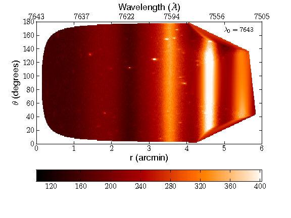
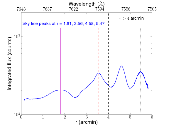
The two-dimensional images are collapsed into one-dimensional spectra by taking the median across all $\theta$ at a given $r$. The example in Figure 3 shows a sky spectrum for an image where the central wavelength is approximately 7643 $\rm\AA$. Comparing Figure 3 to Figure 1, while noting the central wavelength of 7643 $\rm\AA$, implies the visible sky lines in the spectrum correspond to wavelengths 7624.85, 7571.80, 7524.75, and 7477.8 $\rm\AA$. The central wavelength of each sky line in a one-dimensional spectrum is measured simply as the local maximum emission.

Reliable observations in the OSIRIS red TF data are limited to a circular field of view of radius 4 arcmin (960 pixels); beyond 4 arcmin, there can be contamination by other orders. For all sky lines at radii less than 4 arcmin from the optical centre, we measure the expected wavelengths of the sky lines using Equation (1). The average offsets between the actual and expected sky line wavelengths are the requisite adjustments to $\lambda_{0}$ for a single exposure. As a simplification, we calculate average adjustments to $\lambda_{0}$ as a function of tuning wavelength and field. The adjustments were typically $\sim 5$ $\rm\AA$, but they were as high as $\sim$11 $\rm\AA$ in some cases.

In Figure 4 we test whether the updated calibration still follows the relation from González et al. (2014, our Equation 1). We plot $\lambda_{\rm sky}-\lambda_{0}^{\prime}$, where $\lambda_{\rm sky}$ is the sky line wavelength and $\lambda_{0}^{\prime}$ is the recalibrated tuning wavelength, for sky lines within 4 arcmin of the optical centre. The line is the relation from González et al. (2014). Offsets of $\sim 2-3$ $\rm\AA$ from the calibration are common. González et al. (2014) assumed the CS-100 Fabry-Pérot controller in OSIRIS is strictly linear in its gap spacing-control variable (Z) relation, and attributed all non-linearities to phase dispersion effects in the dielectric coatings of the etalons. The discrepancy we measure here may be an indication that the assumption of linearity is not strictly true.

While the relation from González et al. (2014) is accurate over a large wavelength range, systematic offsets up to 3 $\rm\AA$ can occur in certain narrow wavelength ranges. One can proceed with this level of disagreement if it does not affect the accuracy of the science, e.g., H$\alpha$-based star-formation rates. For redshift determinations, however, a 2 $\rm\AA$ error (93 km/s) is large.

We propose an iterative method to refit the wavelength calibration and reduce the typical error down to 1 $\rm\AA$. In our data set, most (89%) exposures with more than one sky line inside 4 arcmin of the optical centre contain the sky line at 7624.85 $\rm\AA$. We focus on these exposures and perform an iterative procedure.

• •

  Calculate offsets relative to the González et al. (2014) calibration for sky line 7624.85 $\rm\AA$ as a function of tuning wavelength setting ($\lambda_{0}$) and field.

• •

  Apply these offsets to the remaining sky lines at wavelengths other than 7624.85 $\rm\AA$. To these sky lines, fit the same functional form justified by González et al. (2014), but with more free parameters for better agreement, namely

  $$\lambda=\lambda_{0}+a_{2}r^{2}+a_{3}(\lambda)r^{3}$$

  (3)

  where

  $$a_{3}(\lambda)=a_{3,0}-1.5698\times 10^{-3}\lambda+1.0024\times 10^{-7}\lambda^{2}.$$

  (4)

  The free parameters are $a_{2}$ and $a_{3,0}$, which are fixed to -5.04 and 6.0396 by González et al. (2014).

• •

  Iterate until the model converges with the sky lines at 7624.85 $\rm\AA$. In subsequent iterations, the offsets for the 7624.85 $\rm\AA$ sky line are calculated relative to the newly fit model in the above step.

Figure 4 shows the result after 10 iterations of this procedure. The fit is noticeably better overall (although residuals for a few measurements slightly worsen). Most (85.5%) of the individual sky line measurements agree to within 1 $\rm\AA$ of the new calibration. This is an improvement over Figure 4 where that percentage is only 50.7% for the González et al. (2014) solution.

Using the new calibration from Figure 4, we calculated average corrections to $\lambda_{0}$ for each combination of wavelength setting and field in our data. Correcting the central wavelengths with the offsets calculated from the sky lines in this way yields a wavelength calibration accurate to within $0.5$ $\rm\AA$ for most (76%) of the individual image frames, and accurate to within $1$ $\rm\AA$ for 95% of the frames. The 1 $\rm\AA$ level of accuracy is a success considering it is $\sim 7\%$ of the 14 $\rm\AA$ instrumental resolution. The calculated corrections do not vary in any systematic way with date of observation, ambient temperature, or humidity. The mean offset does vary weakly with $\lambda_{0}$. The average offset declines from $2$ $\rm\AA$ at $\lambda_{0}=7620$ $\rm\AA$ to $-2.7$ $\rm\AA$ at $\lambda_{0}=7734$ $\rm\AA$.

It is important to point out that OSIRIS uses a non-standard phase correction scheme that may affect the generalisability of this method to very different Fabry-Pérot interferometers. Additional prerequisites for the application of this method are that the data be circularly symmetric around the optical centre and that wavelength dependence on detector position be radially symmetric. Our wavelength recalibration benefited from having a common sky line across most exposures; not having this may produce poorer results. This technique’s accuracy may further be limited by variation in sky line relative intensities, which can perturb the effective peak positions of the blended sky lines in the low-resolution OSIRIS sky spectra. For our TF bandpass ($\sim 14$ $\rm\AA$) and spectral range, the variability is small ($\pm 0.14$ $\rm\AA$), but it may be worse in other instances.

In this section we overview a new sky subtraction technique for TF data. The current sky subtraction in OOPS works by artificially dithering images on a 3-by-3 pixel grid (Ederoclite 2012). Median combining the dithered images produces an estimate of the sky background. Visual inspection of the sky maps, such as the one shown in Figure 5 tuned to a central wavelength of 7615 $\rm\AA$, shows that the outer envelopes of galaxies remain in the sky background. Applying this sky background oversubtracts and eliminates the real outer envelopes of galaxies.

We have developed an alternate approach to sky subtraction that mitigates the problem of source oversubtraction. The basic idea is to remap the flat-fielded images from Cartesian to polar coordinates (Section 3) and then run a median filter, in polar coordinates, along circular arcs of grouped radii, to filter out sources and leave behind an estimate of the sky background.

Circular symmetry in the background sky emission means that the sky changes quickly in $r$ but is relatively stable across $\theta$ at a given $r$ (Figure 3). However, sky subtraction is not as straightforward as converting a collapsed one-dimensional sky spectrum (e.g., Figure 3) into a two-dimensional circularly-symmetric sky model. Because in some cases the sky varies as a slow function of $\theta$ ($5$–$10$% amplitude) due to imperfect flatfielding, this simplified approach is less effective at removing broadened sky line emission than the method we will adopt.

The simplest application of a median filter is to filter over $\theta$ at a given $r$ with a fixed window size (as measured in polar image pixels). This is also not recommended. Sources at small distances from the optical centre are not effectively removed because, for a fixed window size in polar coordinates, the number of pixels from the original image that contribute to the median becomes very small at small radii. A significant improvement in filtering performance is achieved by fixing the median filter window to contain an approximately constant number of pixels from the original image. Thus, for a given filtering window $drd\theta$, the number of polar image pixels in the filter varies inversely with radius, and this ensures a sufficient number of pixels from the original image are filtered over at small radii.

As we show below, changing the width of $d\theta$ has little effect on the outcome of the sky subtraction. Changing $dr$, however, has a more significant effect. Increasing $dr$ incorporates more image pixels into the filter, improving robustness and increasing the speed of the filtering. Raising $dr$ too high yields a sky map with too low spectral resolution that introduces artifacts in the sky-subtracted images. As a compromise, we have chosen to set $dr$ to 3 pixels ($0\hbox{$.\!\!^{\prime\prime}$}75$, 0.57 $\rm\AA$ at $r=4$ arcmin), small enough to be beneficial but not problematic.

Because the dependence of $\lambda$ on $r$ is approximately quadratic, a more sophisticated approach would be to change $dr$ according to quadratically varying bins such that each radial bin represents a constant $\Delta\lambda$ decrement in wavelength. We have tested this binning pattern with our data. Even if we make the radial bins 1 pixel wide at large radii, the radial bins near the optical centre become so wide that often include many sources which are not effectively removed by the median. This leaves behind residual background light in the sky-subtracted images that would bias the photometry of centrally located sources. Other, more complex, radial binning patterns could also be applied, but we did not find they yield any significant improvement over our method. Nevertheless, while this increased complexity is not necessary with our data, it may prove useful with different data sets.

As a further refinement, we apply sigma clipping to prevent the extended halos of bright sources from being smeared into the background sky, which causes local oversubtraction of the sky and leads to dark halos around galaxies. We have found that iteratively clipping to $3\sigma$ for 5 iterations is sufficient to nullify this effect.

Figure 5 shows the results of applying the filtering to the same exposure highlighted in Figure 5. For this example, we have fixed $dr$ to 3 pixels and the total filter size $drd\theta$ to 170 pixel-radians, corresponding to a filter size of 20 degrees at $r=2$ arcmin. The sky background is much smoother than what is provided by the current algorithm in OOPS (Figure 5, left-hand panel), and the sky-subtracted sources in the right-hand panel of Figure 5 are clearly brighter than in Figure 5. Binning in $r$, however, yields sky models with band-like artifacts of width $dr$ (see Figure 6, row 2, column 2). The change in brightness between bands is typically $\sim$1-2% of the sky background, smaller than the background shot noise (3–4%).

Figure 6 gives a magnified view of the sky subtraction in an image subregion containing bright extended objects as well as small faint sources. The sky subtracted-images in the third column emphasise that galaxy light sacrificed by the standard OOPS algorithm is retained with median filtering.

To quantify how much light was gained with the revised sky subtraction procedure, we measured the fluxes of sources in the sky-subtracted images using the methodology of Chies-Santos et al. (2015). Fluxes of galaxies in the right-hand panel of Figure 5 are higher by a median of $\sim 37\%$ versus the OOPS image in Figure 5. This boost in flux is not strongly sensitive to either $dr$ or the total filter size $drd\theta$. We repeated this test for filters with $dr$ values of 1–5 pixels (at fixed $drd\theta$ of 170 pixel-radians), as well as for $drd\theta$ values of 10–30 degrees at $r=2$ arcmin (with $dr=3$ pixels). The resulting median flux ratios deviate by $\sim 1-3\%$ from the $\sim 37\%$ value obtained with the adopted fiducial filter parameters ($dr=3$ pixels, $drd\theta=170$ pixel-radians).

This filtering technique is implemented in Python using standard libraries, including Astropy (Astropy Collaboration et al. 2013). We are assisting with the incorporation of this technique into OOPS so that all users of OSIRIS will have access (Ederoclite, private communication).

In this letter, we have used data from the red TF mode on OSIRIS to demonstrate new techniques for wavelength calibration and sky subtraction. Central to our methodology is the use of polar coordinates, which simplifies matters when the TF data is circularly symmetric. In Section 3, we outlined a technique for wavelength recalibration using OH sky emission rings. This approach increases the accuracy of the absolute wavelength calibration from $\sim 5$ $\rm\AA$ to 1 $\rm\AA$, or $\sim 7\%$ of the instrumental resolution. In Section 4, we presented a new method to estimate the sky background by median filtering in polar coordinates. The merit of this approach is that of light from the extended halos of emission-line galaxies does not contaminate the background sky maps. Sources in the associated sky-subtracted images will likely be significantly brighter than how they would appear in images based on the current sky-subtraction algorithm in the OSIRIS reduction software pipeline, OOPS. Future OSIRIS/OOPS users will benefit from this sky subtraction method.

Based on observations made with the Gran Telescopio Canarias, installed in the Observatorio del Roque de los Muchachos of the Instituto de Astrofísica de Canarias, in the island of La Palma. The GTC reference for this programme is GTC2002-12ESO. Access to GTC was obtained through ESO Large Programme 188.A-2002.

References

- Astropy Collaboration et al. (2013) Astropy Collaboration, Robitaille T. P., Tollerud E. J., et al., 2013, A&A, 558, A33
- (2) Bland-Hawthorn J., 2000, in van Breugel W., Bland-Hawthorn J., eds, ASP Conf. Ser. Vol. 195, Imaging the Universe in Three Dimensions. Astron. Soc. Pac., SanFrancisco, p. 34
- (3) Chies-Santos A. et al., 2015, MNRAS, in press
- (4) Cepa J., Bongiovanni A., Pérez García A. M., et al. 2013, Highlights of Spanish Astrophysics VII, 868
- (5) Cepa J. 2013b, Revista Mexicana de Astronomia y Astrofisica Conference Series, 42, 77
- (6) Ederoclite A., The OSIRIS Offline Pipeline Software (OOPS), 2012
- González et al. (2014) González J. J., Cepa J., González-Serrano J. I., & Sánchez-Portal M. 2014, MNRAS, 443, 3289
- Gray et al. (2009) Gray, M. E., Wolf, C., Barden, M., et al. 2009, MNRAS, 393, 1275
- Osterbrock et al. (1996) Osterbrock, D. E., Fulbright, J. P., Martel, A. R., et al. 1996, PASP, 108, 277