A New Energy Efficient Beamforming Strategy
for MISO Interfering Broadcast Channels
based on Large Systems Analysis
Abstract
In this paper, we propose a new beamforming design to maximize energy efficiency (EE) for multiple input single output interfering broadcast channels (IFBC). Under this model, the EE problem is non-convex in general due to the coupled interference and its fractional form, and thus it is difficult to solve the problem. Conventional algorithms which address this problem have adopted an iterative method for each channel realization, which requires high computational complexity. In order to reduce the computational complexity, we parameterize the beamforming vector by scalar parameters related to beam direction and power. Then, by employing asymptotic results of random matrix theory with this parametrization, we identify the optimal parameters to maximize the EE in the large system limit assuming that the number of transmit antennas and users are large with a fixed ratio. In the asymptotic regime, our solutions depend only on the second order channel statistics, which yields significantly reduced computational complexity and system overhead compared to the conventional approaches. Hence, the beamforming vector to maximize the EE performance can be determined with local channel state information and the optimized parameters. Based on the asymptotic results, the proposed scheme can provide insights on the average EE performance, and a simple yet efficient beamforming strategy is introduced for the finite system case. Numerical results confirm that the proposed scheme shows a negligible performance loss compared to the best result achieved by the conventional approaches even with small system dimensions, with much reduced system complexity.
I Introduction
A design of traditional wireless networks focusing on high spectral efficiency has caused rapidly increasing energy consumption and negative impact on the environment. Therefore, pursuing high energy efficiency (EE) becomes an important and urgent task for future wireless system designs [1]. In general, the EE is defined as the ratio of the sum-rate to the total power consumption measured in bit/Joule. Meanwhile, coordinated beamforming schemes, which allow base stations (BSs) to jointly optimize their transmissions by sharing channel state information (CSI), are considered as a key technology in cellular networks due to its significant spectral efficiency improvement [2]. When the EE is taken into account for a design of future wireless systems, cooperative transmission techniques need to be investigated with new perspectives.
From the EE point of view, several papers have studied methods to maximize the performance various systems [3, 4, 5, 6, 7, 8, 9]. The EE maximization problem in general belongs to a class of fractional programming due to its fractional form, and thus is nonlinear. Nevertheless, for the special case of no interference among users, the problem can be transformed into an equivalent convex problem without loss of optimality by exploiting the pseudo concavity of the objective function [3]. As a result, the global optimal solution can be found efficiently by convex optimization tools [10]. Also, for the multi-user case, the same framework can be adopted by employing zero-forcing beamforming [11], although the resultant performance is suboptimal in terms of EE. However, in more general scenarios with inter-user interference, the optimization problem for EE is non-convex, and thus it is difficult and more challenging to optimize the EE in the presence of interference.
In this paper, we focus on designing a new energy efficient scheme for multi-cell multi-user downlink systems where each BS equipped with multiple antennas communicates with its corresponding single-antenna users. These systems can be mathematically modeled as multiple input single output (MISO) interfering broadcast channels (IFBC). After transforming from fractional programming to linear programming in [3] and applying the weighted minimum mean square error (WMMSE) approach in [12], a local optimal solution was achieved in [5]. However, this method requires either centralized channel knowledge or the exchange of additional parameters. In addition, the optimal beamforming vectors should be computed in an iterative manner for every channel realizations. Moreover, it is difficult to get insights on average performance without resorting to Monte Carlo simulations.
To overcome these issues, we propose a low complexity energy efficient scheme with a negligible performance loss compared to the best results achieved by the conventional approach. To this end, we first parameterize the beam vectors by the parameters associated with beam direction and power. With this parameterization, we then employ the asymptotic results of random matrix theory [13, 14, 15, 16]. More specifically, in the large system limit where the number of transmit antennas and users in each cell go to infinity with a fixed ratio, we identify the parameters to optimize the EE. Note that the beamforming vector which maximizes the EE performance is still constructed based on local instantaneous CSI in a finite dimension. Meanwhile, the parameters can be optimized by adopting the large system analysis. It is worth noting that in the asymptotic regime, the parameters become deterministic and the randomness according to instantaneous channel realizations disappears. Therefore, only second order channel statistics is required for the large system approach.
In [17], the sum rate (SR) maximization is performed for MIMO interference channel by utilizing the fact that a zero gradient value for sum rate maximization under fixed full power is efficiently obtained by utilizing a relationship between the SR and virtual signal-to-interference-plus-noise. However, this method cannot be directly applied for the EE metric since beamforming direction and power allocation are jointly considered for the EE maximization. Different from conventional EE algorithms which should be updated in each channel realization, the proposed method does not recalculate the parameters as long as statistical channel information remains constant. Thus, our long-term strategy significantly reduces complexity and the system overhead compared to the conventional methods. In addition, the dimensionality of the optimization problem is greatly reduced by virtue of the asymptotic approach. Moreover, an asymptotic expression of the achievable EE allows efficient evaluation of the system performance without the need of heavy Monte Carlo simulations. The simulation results demonstrate that the performance of the proposed scheme is almost identical to the near-optimal EE even for small system dimensions, with much reduced computational complexity.
The rest of this paper is organized as follows: Section II describes a system model and the problem formulation. In Section III, we present a low complexity beamforming design based on large system analysis, and simulation results are presented in Section V. Finally, in Section VI, this paper is terminated with conclusions.
Throughout the paper, we adopt uppercase boldface letters for matrices and lowercase boldface for vectors. The superscripts and stand for transpose and conjugate transpose, respectively. In addition, , , and represent 2-norm, trace, the -th element of a vector and the -th entry of a matrix, respectively. Also, denotes an identity matrix of size and means a zero matrix of size . A set of dimensional complex column vectors is defined by and indicates the cardinality of the set .
II System Model

In this paper, we consider an -cell MISO-IFBC with bandwidth where each BS equipped with transmit antennas serves users with a single antenna as shown in Fig. 1. Here user indicates the -th user in cell . Denoting where is a deterministic transmit covariance matrix at the -th BS and as the flat-fading channel vector from the -th BS to the -th user in cell with the coherence time , the received signal at user is expressed by
where equals the beamforming vector for user , stands for the complex data symbol intended for user , and represents the additive white Gaussian noise at user . Throughout the paper, we assume that the entries of are uncorrelated Rayleigh fading according to where indicates the pathloss from BS to user . Note that our result can be easily extended to a more general channel model. It is also assumed that in order to satisfy per-BS power constraint .
We assume single user detection at the receiver so that each receiver treats interference as the Gaussian noise. Thus, the individual rate of user for given transmit beamforming vectors of all BSs is computed as
| (1) |
where represents the individual signal-to-interference-plus-noise ratio (SINR) for user expressed as
| (2) |
Then, the total amount of information transmitted during a time-frequency chunk is given by
Meanwhile, for designing an energy efficient transmission algorithm, we consider the power consumption model for BSs in [6]. Thus, the total energy consumption during the time-frequency block is modeled as
| (3) |
where is a constant associated with the power amplifier inefficiency, is defined by with being the constant circuit power consumption proportional to the number of radio frequency chains, and denotes with accounting for the static power consumed at the BS which is independent of the number of transmit antennas. For example, includes power dissipation in the transmit filter, mixer, frequency synthesizer, and digital-to-analog converter [6].
Accordingly, the EE in bits/Joule is defined as the weighted sum-rate (WSR) divided by the amount of the energy consumption as
| (4) |
Here, it is assumed that the positive weight term is predetermined by a scheduler according to the priority of user [5]. Thus, the EE maximization problem can be formulated as
| (5) | |||
We notice that problem (5) is in general non-convex due to coupled interference among users and its fractional form. Therefore, identifying a solution of this problem is quite complicated. As an alternative, by applying a transformation from the fractional programming into LP and the WMMSE approach sequentially, a local optimal solution can be obtained as in [5].
III Conventional Approach for Energy Efficiency
In this section, we briefly review a conventional approach for the EE maximization in [5], which employs a two-layer optimization strategy. First, in the outer layer, the fractional programming problem is transformed into a linear programming problem with a new parameter. Then, for the given parameter, the inner problem is solved by using the WMMSE method developed in [12]. Eventually, a final solution is found by inner and outer loops iterations.
The optimization problem (5) can be transformed into a linear programming problem by introducing a new parameter . From the relationship between the fractional programming and the parametric programming [3], the original problem (5) can be recast as the following equivalent form
| (6) | |||||
| s.t. | |||||
For a fixed value of , we have a feasibility problem in which checks if , where indicates the optimal value of the following problem
| (7) | |||||
| s.t. |
From Theorem 1 in [5], is shown to be a monotonically decreasing function with respect to and the equation has a unique solution. As a result, the optimal value of can be identified using one dimensional search algorithms such as a simple bisection method [10].
Next, the optimal beamforming needs to be determined in the inner problem for a fixed . For the given , the inner problem (7), excluding terms irrelevant to the optimization variables , is rephrased as
| (8) | |||||
| s.t. |
where .
Note that this problem is quite similar to the SR maximization problem except for the power term in the objective function. Thus, using the relationship between the SR and the WMMSE, a solution of the problem (8) can be computed from the following equivalent problem
| (9) | |||||
| s.t. |
where the mean square error is given by
| (10) |
and and are auxiliary variables.
The above problem is still non-convex in terms of jointly, making the direct optimization of the problem difficult. However, since the problem is convex with respect to each of the optimization variables and , we can solve the problem with one parameter by fixing the other two, i.e., the problem can be calculated by alternating the optimization method. For given , the optimal of the problem (9) is obtained by
| (11) |
Furthermore, for fixed and , the optimal is expressed by
| (12) |
Then, once the values of and are given, the optimization of is decoupled among the BSs by substituting in (10) into the objective function of the problem (9), and this leads to the following distributed optimization problems for the -th BS
| (13) | |||||
| s.t. |
Denoting as the Lagrange multiplier corresponding to the power constraint, the first order optimality condition of the Lagrange function with respect to each yields
| (14) |
where is chosen such that the complementary slackness condition of power constraint is fulfilled. Let be the right-hand side of (14). If , then . Otherwise, can be found by using the bisection method which satisfies . Therefore, a solution of for a given can be computed by updating and in an alternating fashion.
In summary, a local optimal point of the EE can be determined by two-layer optimization. However, the algorithm should be carried out in an iterative manner per each instantaneous channel realization by sharing global channel information among BSs. This leads to high computational complexity and signaling overhead. In the following, we will propose a new algorithm with low complexity and overhead which is more desirable in practical systems.
IV Proposed EE Scheme based on Large System Analysis
In this section, we propose an energy efficient scheme with low complexity in a finite dimension. After introducing conventional approaches, we describe the proposed method based on the asymptotic results of random matrix theory. Note that we consider the asymptotic regime where with held at a fixed ratio to quantify beamforming parameters. The key idea is to combine large system analysis techniques with the WMMSE approach. Specifically, by applying the equivalence property between SR and WMMSE, the structure of the optimal beamforming vector is characterized with parameters related to beam direction and power. Then, by employing the asymptotic results of random matrix theory, the value of the parameters becomes deterministic which depends only on the second order channel statistics, and this leads to a significant reduction in the computational complexity compared to the system which utilizes instantaneous CSI. As will be shown later, the beamforming vector can be computed using only the optimized parameters and local CSI.
Before explaining the algorithm, we provide useful results for solving the problem. First, we identify the structure of the optimal beamforming based on in (14). Note that from , the structure of beamforming can be paramterized with the power term and the parameters related to the beam direction and as
| (15) |
where and are given as
| (16) | |||||
| (17) |
and and are denoted as and , respectively. Based on this structure, the normalized beam direction vectors is defined as
| (18) |
where and represent the parameters which control the leakage interference power level to other users adaptively.
In order to quantify the component-wise impact on the performance for the given beamforming vectors , we introduce the normalized channel gain matrix as
| (19) |
As mentioned before, in order to compute these instantaneous channel gains in a finite dimension, we exploit the results of the RMT for an asymptotic region. The -th off-diagonal element of accounts for interference power at user generated by the -th BS for serving its supporting user , and the diagonal elements stand for the desired signal power. Employing the asymptotic results of random matrix theory, we arrive at the following lemma.
Lemma 1
For fixed ratio with , the deterministic equivalent of is obtained as
| (20) |
where
| (21) |
Here, and are given by
| (22) | |||||
| (23) |
where and are provided in the proof.
Proof:
See Appendix A. ∎
With , the deterministic equivalent of is derived as
| (24) |
where
| (25) |
Here, represents the -th element of . By the continuous mapping theorem [18], one can show that the deterministic equivalents of the SR and the EE are expressed as
| (26) | |||||
| (27) |
In what follows, based on the above asymptotic results, we optimize the EE performance in the large system limit instead of the original problem (5). The EE problem in the asymptotic regime is formulated as
| (28) | |||||
| s.t. |
In the outer layer optimization, our algorithm is analogous to the conventional approach shown in Section III. However, unlike the conventional approach adopting a short-term strategy, we consider a long-term strategy in order to achieve low complexity. Notice that for the finite dimensional case, the outer layer algorithm is required only to generate and pass to the inner problem. Then, is updated according to the feasibility, i.e., or not, based on a solution of the inner problem. Similar to the finite case, the feasibility in the asymptotic regime can be determined whether or not, where is the optimal value of the following problem
| (29) | |||||
| s.t. |
Now, the only remaining work in the outer layer optimization is to identify the maximum value of for a bisection method. It is clear that the maximum value can be obtained as
| (30) |
Thus, applying Theorem 3.4 in [19], it follows
| (31) |
where we have used .
Next, we derive the optimal beamforming in the inner problem for a fixed . Similar to (8), the objective function in the problem (29) can be reduced to
| (32) |
Then, by utilizing the WMMSE approach, the problem (29) can be recast as
| (33) | |||||
| s.t. |
where the mean square error is given by
Thus, for any given , the optimal receiver filters of the problem (33) are obtained by
| (34) |
Furthermore, the optimal is expressed by
| (35) |
It is obvious that the optimal in (33) is equal to from (16) for the finite case. Thus, we can calculate new based on the updated .
Next, for given and , the distributed problem for the -th BS in the large system regime becomes
| (36) | |||||
| s.t. |
Then, the optimal transmit power is written by
| (37) |
Here, from (17), is equal to where is determined by the complementary slackness of power constraint.
IV-A Overall Algorithm and Complexity Analysis
The Algorithm 1 and 2 describe the overall procedure of the proposed scheme. Here, indicates a predefined threshold. It is worth noting that our proposed algorithm depends only on the second channel statistics, and not on instantaneous channel realizations. More specifically, the conventional method determines and per each channel realization, while the proposed algorithm does so only when the second order statistics changes, i.e., signal-to-noise ratio (SNR) changes. Once the optimal and are determined, we can construct the beamforming vectors based only on local CSI without additional complexity. Thus, the proposed algorithm dramatically reduces the computational complexity compared to the conventional scheme.
In what follows, we compare the complexity of the conventional scheme with that of the proposed method. For comparison, the overall computational complexity can be characterized by the multiplication of the following terms: the execution rate of the algorithm, the iteration number of the outer layer, the iteration number of the inner layer, and the complexity of inner layer optimization per each iteration. Here, the per-iteration complexity of the outer layer optimization is ignored since the calculation using the bisection method is relatively simple.
First, the per-iteration computational complexities of the conventional scheme and the proposed method are and , respectively. The difference between the two schemes comes from an inverse operation of an matrix. The conventional algorithm requires the inverse operation to generate the beamforming vectors in (14), while the proposed scheme does not need as can be seen in Algorithm 2. Thus, a complexity gain becomes larger as increases. Next, for the inner and outer layer algorithm, the required number of iterations of both schemes are quite similar in average sense, since both of them are based on the bisection method and the WMMSE algorithm.
Compared to the conventional scheme, the factor which reduces the complexity the most in the proposed algorithm is the execution rate of the overall algorithm. The update rate of the proposed algorithm depends on how often the second order channel statistics changes, and thus is much slower than that of the conventional method which needs to update at each realization. This is because large scale fading varies with tens of seconds, while small scale fading changes with few milliseconds in general wireless environments [20]. Thus, the coherence time of small scale fading is typically 1000 times smaller than that of large scale fading. As a result, for example, with , , and , the CPU running time of the conventional EE algorithm is about 300 times more than that of the proposed scheme. Therefore, we can verify that the proposed algorithm greatly reduces the computational complexity compared to the conventional scheme. We shall show in the simulation section that our proposed algorithm exhibits the performance almost identical to that of the conventional algorithm while requiring significantly reduced complexity.
V Numerical results
| System bandwidth () | 20 MHz |
|---|---|
| The number of user drops | 10 |
| The number of channel realizations per user drop | 100 |
| The number of Tx antennas for each BS | 4 |
| Cell radius | 500 m |
| Minimum distance from BS to each user | 35 m |
| Pass loss exponent | 3.8 |
| Transmit power constraint per BS | 26 46 dBm |
| Circuit power per antenna | 30 dBm |
| Basic power consumed at BS | 40 dBm |
| Noise figure () | 7 dB |
| Noise power | -94 dBm |
| Inefficiency of the power amplifier | 2 |
In this section, we evaluate the EE performance of the proposed beamforming scheme. We consider a cooperative cluster of hexagonal cells for Monte Carlo simulations. These simulations are carried out with the parameters listed in Table I, unless specified otherwise. The pathloss from BS to user is given as in decibels, where in meter indicates the distance from BS to user . Also, the noise power can be calculated as in dBm where means the system bandwidth and denotes the noise figure.

First, we illustrate the convergence of the proposed algorithm. For the case of the outer layer optimization, the optimal can be found based on one dimensional line search without loss of optimality, and thus the convergence is guaranteed. On the other hand, the inner layer algorithm cannot achieve the global optimal value due to the non-convexity of the problem. However, the convergence to a local optimal point is guaranteed by virtue of the WMMSE approach [21]. Fig. 2 plots the objective function in (32) with respect to the number of iterations for . The convergence trend varies with parameters such as power, user position and . In this figure, the curves corresponding to 5 different user drop events are plotted by fixing certain and dBm. As shown in this plot, the inner layer algorithm converges to a stable point with about 10 iterations.

Fig. 3 exhibits the average EE performance of various beamforming schemes as a function of for with . For comparison, we first present the EE performance of the following beamforming schemes.
- •
Maximal ratio transmission (MRT): the beamformers are aligned with the corresponding channels.
- •
Zero-forcing beamforming (ZFBF): the signal to unintended users is nullified.
- •
- •
WMMSE algorithm: beamformers are designed to maximize the SR by using the WMMSE approach [12].
- •
Conventional EE algorithm: the algorithm based on the WMMSE approach is adopted to maximize EE as described in Section III.
- •
Proposed EE algorithm: the proposed algorithm performs with adaptive control of and based on second order channel statistics for the EE maximization.
For both the WMMSE and the conventional EE schemes which achieve the local optimal solution, a solution of the VSINR scheme is adopted as an initial point. Surprisingly, we can see that the proposed scheme achieves near-optimal performance with much reduced complexity for all simulated transmit power constraint ranges. It is emphasized again that our proposed algorithm is performed only when second order channel statistics changes and the constant values of and are employed for generating beamforming vectors as long as the statistics remains unchanged. This results in a significant computational complexity reduction compared to the conventional EE scheme which should be carried out in every channel realizations. Moreover, we can observe the trade-off relationship between the performance and the complexity for various beamforming strategies. Simple beamforming schemes such as MRT, ZFBF, and VSINR require lower computational complexity to comprise the beamforming structure than the proposed scheme but with poor performance. In the ZFBF case, the EE performance is mainly degraded by the deficiency of dimension for nullifying the unintended user signals. We also observe that the WMMSE schemes designed for spectral efficiency maximization produce much worse EE performance compared to the proposed scheme. Especially, a performance gain of the proposed EE scheme is about at dBm .
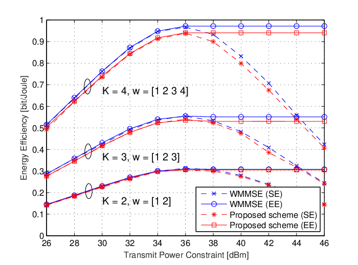
Also, the average EE performance for the conventional and proposed EE algorithms is illustrated for various number of users in Fig. 4. We can see that the EE performance of these two algorithms increases with the number of users. Moreover, the performance of the proposed EE algorithm has a small gap compared to the conventional algorithm, which is less than for all cases.

In Fig. 5, we demonstrate the EE performance of the proposed scheme for the correlated transmit antenna case. The transmit covariance matrix is set as the exponential correlation model which is given by with and . In this correlation model, the average EE performance is enhanced when the correlation coefficient grows at a high transmit power region. On the contrary, the opposite trend is observed at a low transmit power region. This is due to the fact that the EE performance can be mainly affected by an array gain at the low power region. For the high BS power region, the effect of spatial multiplexing takes a key role of the EE performance.

In what follows, we validate the accuracy of the deterministic equivalent of EE compared to true EE. Fig. 6 compares the average EE with the deterministic approximation for and with the fixed ratio . In this plot, each curve corresponds to a particular drop of users for each . The error bars indicate the standard deviation of the simulation results. As shown in this plot, the deterministic equivalent of EE provides a very accurate approximation. It can be seen that the approximation lies within one standard deviation of the Monte Carlo simulations and the standard deviation becomes smaller as increases. Also, we can check that the maximum value of EE gets larger as grows. This comes from an increased multiplexing gain, (i.e. pre-log term) as and grow larger. From the plots, it is observed that the EE performance curve increases up to a certain point, and after that it is saturated. Investigation of the saturation point will be an interesting future work.
VI Conclusions
In this paper, we have proposed a low complexity beamforming scheme for MISO-IFBC. With the parametrization of the beamforming vectors by the scalar values, we have found the optimal parameters to maximize the EE in the asymptotic regime. Our solutions depend only on second order channel statistics, not on instantaneous CSI, and thus the parameters are computed only when channel statistics changes. As a result, the computational complexity is significantly reduced compared to the conventional method. Through simulations, we have confirmed that the proposed schemes with the asymptotic results provide the near-optimal EE performance even for the finite system case. Additionally, the proposed scheme allows efficient calculation of the system performance without resorting to heavy Monte Carlo simulations.
Appendix A Proof of Lemma 1
We will derive the deterministic equivalents of the desired signal power and the interference power subsequently as in [17]. For simplicity, we assume .
A-1 Deterministic equivalent for
For given and , is written by
| (39) | |||||
where , and the last equality comes from the Sherman-Morrison matrix inversion lemma.
First, applying Theorem 3.4 in [19] to the term in the numerator of (39) yields
| (40) |
where . By employing Theorem 1 in [24], it follows
| (41) |
where and with . Here, is defined as
| (42) |
where equals a set with non-negative elements for , represents a positive scalar value and ’s are unique positive solutions of the fixed-point equations
| (43) |
A-2 Deterministic equivalent for
The interference term can be written as
| (48) | |||||
where and the second and third equality come from the Sherman-Morrison matrix inversion lemma with respect to and , respectively.
References
- [1] Y. Chen, S. Zhang, , S. Xu, and G. Y. Li, “Fundamental Trade-offs on Green Wireless Networks,” IEEE Communications Magazine, vol. 49, pp. 30–37, June 2011.
- [2] W. Lee, I. Lee, J. S. Kwak, B.-C. Ihm, and S. Han, “Multi-BS MIMO Cooperation: Challenges and Practical Solutions in 4G Systems,” IEEE Wireless Communications, vol. 19, pp. 89–96, February 2012.
- [3] C. Isheden, Z. Chong, E. Jorswieck, and G. Fettweis, “Framework for Link-Level Energy Efficiency Optimization with Informed Transmitter,” IEEE Transactions on Wireless Communications, vol. 11, pp. 2946–2957, August 2012.
- [4] H. Kim, E. Park, H. Park, and I. Lee, “Beamforming and Power Allocation Designs for Energy Efficiency Maximization in MISO Distributed Antenna Systems,” IEEE Communications Letters, vol. 17, pp. 2100–2103, November 2013.
- [5] S. He, Y. Huang, S. Jin, and L. Yang, “Coordinated Beamforming for Energy Efficient Transmission in Multicell Multiuser Systems,” IEEE Transactions on Communications, vol. 61, pp. 4961–4971, December 2013.
- [6] D. W. K. Ng, E. S. Lo, and R. Schober, “Energy-efficient resource allocation in OFDMA systems with large numbers of base station antennas,” IEEE Transactions on Wireless Communications, vol. 11, pp. 3292–3304, September 2012.
- [7] ——, “Energy-Efficient Resource Allocation in Multi-Cell OFDMA Systems with Limited Backhaul Capacity,” IEEE Transactions on Wireless Communications, vol. 11, pp. 3618–3631, October 2012.
- [8] E. Björnson, M. Kountouris, and M. Debbah, “Massive MIMO and small cells: Improving energy efficiency by optimal soft-cell coordination,” in Proc. 20th International Conference on Telecommuincations, May 2013.
- [9] H. Q. Ngo, E. G. Larsson, and T. L. Marzetta, “Energy and Spectral Efficiency of Very Large Multiuser MIMO Systems,” IEEE Transactions on Communications, vol. 61, pp. 1436–1449, April 2013.
- [10] S. Boyd and L. Vandenberghe, Convex Optimization. Cambridge University Press, 2004.
- [11] E. Björnson, L. Sanguinetti, J. Hoydis, and M. Debbah, “Optimal Design of Energy-Efficient Multi-User MIMO Systems: Is Massive MIMO the Answer?” IEEE Transactions on Wireless Communications, 2014, Submitted. [Online]. Available: http://arxiv.org/pdf/1403.6150v2.pdf.
- [12] Q. Shi, M. Razaviyayn, Z.-Q. Luo, and C. He, “An Iteratively Weighted MMSE Approach to Distributed Sum-Utility Maximization for a MIMO Interfering Broadcast Channel,” IEEE Transactions on Signal Processing, vol. 59, pp. 4331–4340, September 2011.
- [13] R. Zakhour and S. V. Hanly, “Min-Max Power Allocation in Cellular Networks with Coordinated Beamforming,” IEEE Journal on Selected Areas in Communications, vol. 31, pp. 287–302, February 2013.
- [14] R. Couillet, S. Wagner, and M. Debbah, “Asymptotic Analysis of Correlated Multi-Antenna Broadcast Channels,” in Proc. IEEE WCNC, April 2009.
- [15] H. Huh, S.-H. Moon, Y.-T. Kim, I. Lee, and G. Caire, “Multi-Cell MIMO Downlink with Cell Cooperation and Fair Scheduling: A Large-System Limit Analysis,” IEEE Transactions on Information Theory, vol. 57, pp. 7771–7786, December 2011.
- [16] J. Hoydis, S. ten Brink, and M. Debbah, “Massive MIMO in the UL/DL of Cellular Networks: How Many Antennas Do We Need?” IEEE Journal on Selected Areas in Communications, vol. 31, pp. 160–171, February 2013.
- [17] S.-R. Lee, H.-B. Kong, H. Park, and I. Lee, “Beamforming Designs Based on an Asymptotic Approach in MISO Interference Channels,” IEEE Transactions on Wireless Communications, vol. 12, pp. 6430–6438, December 2013.
- [18] P. Billingsley, Probability and Measure. 3rd ed. NewYork: Wiley, 1995.
- [19] R. Couillet and M. Debbah, Random Matrix Methods for Wireless Communications. 1st ed. Cambridge University Press, 2011.
- [20] D. Tse and P. Viswanath, Fundamentals of Wireless Communication. Cambridge University Press, 2005.
- [21] M. V. Solodov, “On the convergence of constrained parallel variable distribution algorithms,” SIAM Joulnal on Optimization, vol. 8, pp. 187–196, February 1998.
- [22] R. Zakhour and D. Gesbert, “Distributed Multicell-MISO Precoding Using the Layered Virtual SINR Framework,” IEEE Transactions on Wireless Communications, vol. 9, pp. 2444–2448, August 2010.
- [23] S.-H. Park, H. Park, H. Kong, and I. Lee, “New beamforming techniques based on virtual SINR maximization for coordinated multi-cell transmission,” IEEE Transactions on Wireless Communications, vol. 11, pp. 1034–1044, March 2012.
- [24] S. Wagner, R. Couillet, M. Debbah, and D. T. M. Slock, “Large System Analysis of Linear Precoding in Correlated MISO Broadcast Channels Under Limited Feedback,” IEEE Transactions on Information Theory, vol. 58, pp. 4509–4537, July 2012.