跳到论文正文
W Papers独立论文阅读器 arXiv:1508.06553 论文正文 计算阅读时间 · 0%
引用这篇论文根据当前论文元数据生成,正式投稿前建议核对。


License: arXiv.org perpetual non-exclusive license
arXiv:1508.06553v1 [physics.atom-ph] 24 Aug 2015

Stereochemical properties of the OH molecule in combined electric and magnetic fields: analytic results

Stefano Marin and Mishkatul Bhattacharya Affiliation: School of Physics and Astronomy, Rochester Institute of Technology, 84 Lomb Memorial Drive, Rochester, NY 14623, USA
August 24, 2026
Abstract

The stereochemical properties of the ultracold ground state OH molecule in the presence of electric and magnetic fields are currently of considerable interest. For example, relevant quantities such as molecular alignment and orientation, calculated numerically by using large basis sets, have lately appeared in the literature. In this work, based on our recent exact solution to an effective eight-dimensional matrix Hamiltonian for the molecular ground state, we present analytic expressions for the stereochemical properties of OH. Our results require the solution of algebraic equations only, agree well with the aforementioned fully numerical calculations, provide compact expressions for simple field geometries, allow ready access to relatively unexplored parameter space, and yield straightforwardly higher moments of the molecular axis distribution.

1 Introduction

The ultracold ground state X2​Π3/2X^{2}\Pi_{3/2} OH molecule is a versatile enabler for studies of spectroscopy [1], precision measurement [2, 3, 4], trapping [5], slowing [6, 7], state transfer [8], cold chemistry [9, 10, 11, 12, 13], and quantum degeneracy [14]. The molecular ground state is polar as well as paramagnetic, and thus many theoretical [15, 16, 18, 19, 20, 21] and experimental [22] studies have focused on the behavior of ultracold OH in combined electric and magnetic fields.

Recently, the stereochemical properties of cold molecules have come under investigation, due to their importance for cold chemistry [23, 24, 25] and molecular beam manipulation [26], for example. Particularly relevant is the work by Gärttner et al. [27], who have calculated the OH molecular axis alignment and orientation by numerically solving the time-independent Schrodinger equation using large sets of basis functions. While such numerical investigations lead to accurate and comprehensive characterization of the OH properties, analytical studies have also provided a fruitful line of investigation in the past, yielding physical insight as well as mathematical compactness [15, 16, 18, 17]. In particular, it has been found that experimental data on Landau-Zener transitions [8] as well as evaporative cooling [14] can be accurately modeled using an eight-level characterization of the ground state OH molecule in crossed electric and magnetic fields [15]; we have recently analytically diagonalized the corresponding Stark-Zeeman matrix Hamiltonian with the assistance of an underlying chiral symmetry [19, 20].

In this article, we exploit the availability of this solution to calculate analytical expressions for the alignment and orientation of the ground state OH molecule. We find good agreement between our analytical results and the existing numerical calculations, indicating the reliability of our expressions. We present our results in order of increasing complexity, by first considering simple field geometries. These yield quite compact expressions - which are exact within the framework of the effective matrix Hamiltonian - for the stereochemical properties. Subsequently, we consider more complicated configurations, where some approximate but useful expressions are presented. Then we show that our full expressions can be used to directly investigate relatively unexplored parameter regimes, such as variation in the angle between the two fields. Finally, we demonstrate that higher order moments of the molecular axis distribution [28] can also be found simply using our approach.

The remainder of this paper is arranged as follows. Section 2 establishes the formalism using the effective Hamiltonian, Section  3 discusses the stereochemical properties, and Section  4 supplies the conclusions.

2 Formalism

In this section we outline the formalism used to calculate the OH stereochemical properties. We first recapitulate the ground state matrix OH Hamiltonian derived originally by Lara et al. [15], for the system shown in Fig. 1.

Refer to caption
Figure 1: Schematic of the diatomic OH molecule in external magnetic (B)(B) and electric (E)(E) fields. The magnetic field has been chosen to lie along the laboratory zz axis and the electric field on the x−zx-z plane, making an angle θ\theta with the zz axis. The angle between the laboratory zz and molecular axes is labelled Θ\Theta and is the main interest of this paper.

The Hamiltonian neglects hyperfine structure and spin-orbit interactions, is valid for strong, but not ultrastrong electric and magnetic fields, and accounts for the Lambda-doublet in the ground OH rotational state

H=Ho−μ→e⋅E→−μ→b⋅B→.H=H_{o}-\vec{\mu}_{e}\cdot\vec{E}-\vec{\mu}_{b}\cdot\vec{B}. (1)

In Equation  (1), HoH_{o} is the field-free Hamiltonian, the second term accounts for the Stark interaction and the third term corresponds to the Zeeman interaction. The symbol μ→e​(μ→b)\vec{\mu}_{e}(\vec{\mu}_{b}) stands for the molecular electric (magnetic) dipole moment, and E→​(B→)\vec{E}(\vec{B}) is the static electric (magnetic) field. To represent this Hamiltonian in matrix form, we use the Hund’s case (a) parity basis |J,M,Ω¯,ϵ⟩|J,M,\bar{\Omega},\epsilon\rangle following Lara et al. [15], where J=3/2J=3/2 is the rotational angular momentum, MM is its projection in the laboratory frame, Ω¯\bar{\Omega} is its projection on the internuclear axis, and ϵ={e,f}\epsilon=\{e,f\} is the e−fe-f symmetry. In this representation, the Hamiltonian reads [18]

HM=(A1−A2−C−CA1+A2),H_{M}=\left(\begin{array}[]{cc}A_{1}-A_{2}&-C\\ -C&A_{1}+A_{2}\\ \end{array}\right), (2)

with

A1=25​μB​B\displaystyle A_{1}=\frac{2}{5}\mu_{B}B (−30000−10000100003),\displaystyle\left(\begin{array}[]{cccc}-3&0&0&0\\ 0&-1&0&0\\ 0&0&1&0\\ 0&0&0&3\\ \end{array}\right),
A2=ℏ​Δ2\displaystyle A_{2}=\frac{\hbar\Delta}{2} (1000010000100001),\displaystyle\left(\begin{array}[]{cccc}1&0&0&0\\ 0&1&0&0\\ 0&0&1&0\\ 0&0&0&1\\ \end{array}\right),
C=μe​E5\displaystyle C=\frac{\mu_{e}E}{5} (−3​cos⁡θ3​sin⁡θ003​sin⁡θ−cos⁡θ2​sin⁡θ002​sin⁡θcos⁡θ3​sin⁡θ003​sin⁡θ3​cos⁡θ),\displaystyle\left(\begin{array}[]{cccc}-3\cos\theta&\sqrt{3}\sin\theta&0&0\\ \sqrt{3}\sin\theta&-\cos\theta&2\sin\theta&0\\ 0&2\sin\theta&\cos\theta&\sqrt{3}\sin\theta\\ 0&0&\sqrt{3}\sin\theta&3\cos\theta\\ \end{array}\right),

where the Lambda-doubling parameter is denoted by Δ\Delta, the Bohr magneton by μB\mu_{B}, the magnitude of the molecular electric dipole moment by μe\mu_{e}, the electric and magnetic field magnitudes by E=|E→|E=|\vec{E}| and B=|B→|B=|\vec{B}|, respectively, and the angle between the magnetic and electric field vectors by θ\theta. For convenience, below we will use the quantities

E~=μe​E,B~=μB​B,Δ~=ℏ​Δ,\tilde{E}=\mu_{e}E,\,\tilde{B}=\mu_{B}B,\,\tilde{\Delta}=\hbar\Delta, (15)

all of which have dimensions of energy. The numerical values of the relevant constants are μe=1.66\mu_{e}=1.66D, μB=9.27×10⁻²⁴\mu_{B}=9.27\times 10^{-24}JT-1 and Δ=2​π×1.67\Delta=2\pi\times 1.67GHz.

The eigenvalues of the eight-dimensional matrix HMH_{M} of Eq. (2) can be found analytically, as shown earlier [19]. For the calculations in this article, we used the commercial software package Mathematica to find the eigenstates of HMH_{M} analytically. The typical form of the OH eigenstate is

|ψ⟩=1N​|c1,c2,c3,c4,c5,c6,c7,c8⟩,\ket{\psi}=\frac{1}{N}\ket{c_{1},c_{2},c_{3},c_{4},c_{5},c_{6},c_{7},c_{8}}, (16)

where the cic_{i} are the components in the Hund’s case (a) parity basis, and the normalization is given by

N=∑i=18ci2.N=\sqrt{\sum_{i=1}^{8}c_{i}^{2}}. (17)

The cic_{i}’s, which are always real, and are somewhat large in form, have been provided in Appendix A.

3 Stereochemical properties

In this section we present our analytical results for the OH stereochemical properties. We consider the expressions for quantities of the form ⟨cosk⁡Θ⟩\langle\cos^{k}\Theta\rangle, which include the orientation (k=1)(k=1), alignment (k=2)(k=2) as well as higher moments (k=3,4)(k=3,4) of the molecular axis distribution [28]. The angle Θ\Theta refers to the inclination of the molecular axis with respect to the laboratory zz axis, see Fig.1. Using the matrix elements of cos⁡Θ\cos\Theta in the Hund’s case (a) basis from Sharma et al. [25], we find, for the eigenstate of Eq. (16),

⟨cos⁡Θ⟩=−25​N2​(3​c1​c5+c2​c6−c3​c7−3​c4​c8),\langle\cos{\Theta}\rangle=-\frac{2}{5N^{2}}\left(3c_{1}c_{5}+c_{2}c_{6}-c_{3}c_{7}-3c_{4}c_{8}\right), (18)
⟨cos2⁡Θ⟩=115​N2\displaystyle\langle\cos^{2}{\Theta}\rangle=\frac{1}{15N^{2}} [7(c12+c42+c52+c82)\displaystyle\left[7\left(c_{1}^{2}+c_{4}^{2}+c_{5}^{2}+c_{8}^{2}\right)\right. (19)
+3(c22+c32+c62+c72)],\displaystyle\left.+3\left(c_{2}^{2}+c_{3}^{2}+c_{6}^{2}+c_{7}^{2}\right)\right],
⟨cos3⁡Θ⟩=−225​N2​(7​c1​c5+c2​c6−c3​c7−7​c4​c8),\langle\cos^{3}{\Theta}\rangle=-\frac{2}{25N^{2}}\left(7c_{1}c_{5}+c_{2}c_{6}-c_{3}c_{7}-7c_{4}c_{8}\right), (20)
⟨cos4⁡Θ⟩=11225​N2\displaystyle\langle\cos^{4}{\Theta}\rangle=\frac{1}{1225N^{2}} [289(c12+c42+c52+c82)\displaystyle\left[289\left(c_{1}^{2}+c_{4}^{2}+c_{5}^{2}+c_{8}^{2}\right)\right. (21)
+89(c22+c32+c62+c72)].\displaystyle\left.+89\left(c_{2}^{2}+c_{3}^{2}+c_{6}^{2}+c_{7}^{2}\right)\right].

In the interest of readability, we start by considering simple geometries for which we find compact analytic expressions, and then move on to more general cases. Readers who wish to first convince themselves that our analytic expressions match well with previous numerical calculations may refer to Section 3.5, especially Fig. 6, directly.

3.1 Magnetic Field Only

We start by considering the orientation and alignment in the presence of a magnetic field only,

⟨cos⁡Θ⟩=0,for all states,\langle\cos{\Theta}\rangle=0,\,\,\text{for all states,} (22)
⟨cos2⁡Θ⟩=130​(4​M2+5).\langle\cos^{2}{\Theta}\rangle=\frac{1}{30}\left(4M^{2}+5\right). (23)

Thus, all states with M=±3/2M=\pm 3/2 have ⟨cos2⁡Θ⟩=7/15\langle\cos^{2}{\Theta}\rangle=7/15, whereas for M=±1/2M=\pm 1/2, ⟨cos2⁡Θ⟩=1/5\langle\cos^{2}{\Theta}\rangle=1/5. We see that the magnetic field does not affect either of these stereochemical properties; this is because the Zeeman terms in Eq. (1) are diagonal in the Hund’s case (a) basis, and therefore do not influence the components of the eigenstate [Eq. (16)] at all. The presence of a magnetic field is thus equivalent to the field-free case.

3.2 Electric field only

We now consider the orientation and alignment in the presence of an electric field only. In this case, it is convenient to rotate the electric field to the laboratory zz axis in Fig.  1. While general expressions applying to all states can easily be given, for the sake of illustration, we discuss the properties of the lowest energy state |ψg⟩\ket{\psi_{g}}. In the presence of an electric field this state is given by

|ψg⟩=1N​|0,0,−−5​Δ~−25​Δ~2+4​E~22​E~,0,0,0,1,0⟩,\displaystyle\ket{\psi_{g}}=\frac{1}{N}\ket{0,0,-\frac{-5\tilde{\Delta}-\sqrt{25\tilde{\Delta}^{2}+4\tilde{E}^{2}}}{2\tilde{E}},0,0,0,1,0}, (24)

in the Hund’s case (a) parity basis with

N=2+5​Δ~​(5​Δ~+25​Δ~2+36​E~2)18​E~2.N=\sqrt{2+\frac{5\tilde{\Delta}\left(5\tilde{\Delta}+\sqrt{25\tilde{\Delta}^{2}+36\tilde{E}^{2}}\right)}{18\tilde{E}^{2}}}. (25)

A straightforward calculation yields the orientation

⟨cos⁡Θ⟩=18​E~5​25​Δ~2+36​E~2,\langle\cos{\Theta}\rangle=\displaystyle\frac{18\tilde{E}}{5\sqrt{25\tilde{\Delta}^{2}+36\tilde{E}^{2}}}, (26)

and the alignment

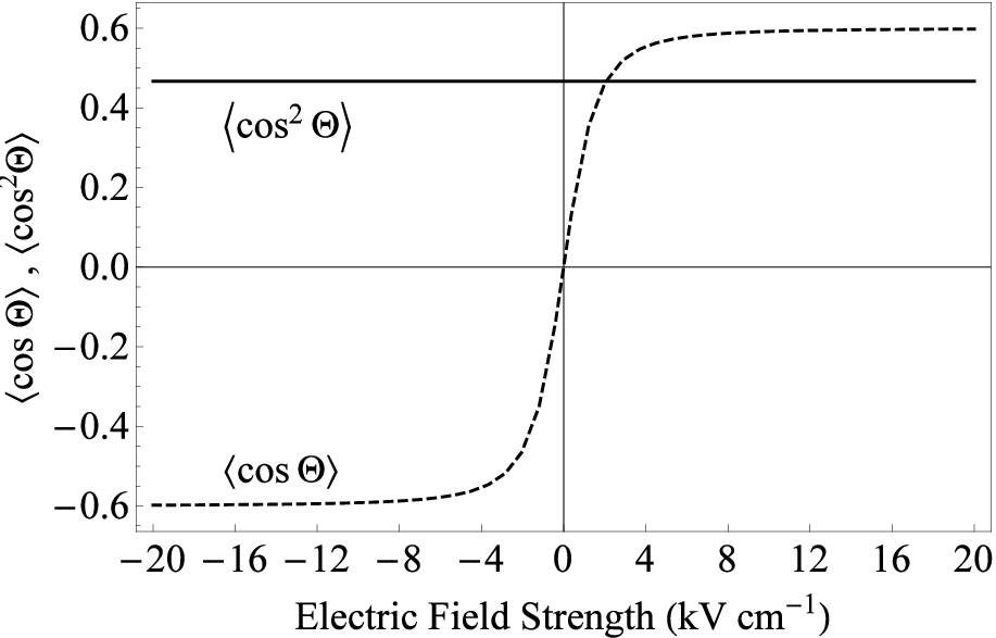
⟨cos2⁡Θ⟩=715.\langle\cos^{2}{\Theta}\rangle=\displaystyle\frac{7}{15}. (27)

The alignment is independent of the electric field due to the presence of chiral symmetry [20]. The orientation, as can be seen from the property

∂⟨cos⁡Θ⟩∂E~=90​Δ~2(25​Δ~2+36​E~2)3/2,\frac{\partial\langle\cos{\Theta}\rangle}{\partial\tilde{E}}=\frac{90\tilde{\Delta}^{2}}{\left(25\tilde{\Delta}^{2}+36\tilde{E}^{2}\right)^{3/2}}, (28)

increases monotonically with the electric field, and reaches an asymptotic value of

limE~→∞⟨cos⁡Θ⟩=35.\lim_{\tilde{E}\rightarrow\infty}\langle\cos{\Theta}\rangle=\frac{3}{5}. (29)

The orientation and alignment have been plotted versus the electric field in Fig. 2.

Refer to caption
Figure 2: ⟨cos⁡Θ⟩\langle\cos{\Theta}\rangle (dashed), ⟨cos2⁡Θ⟩\langle\cos^{2}{\Theta}\rangle (solid) for B=0B=0 as a function of the electric field.

3.3 Parallel fields

As we have shown in Section 3.1, a magnetic field along the laboratory zz axis does not influence the orientation or alignment. If, in addition, an electric field is introduced the same direction (i.e. θ=0\theta=0 in Fig. 1), then for these parallel fields the results of Section 3.2 apply. In other words, only the electric field has an effect on the stereochemical properties of the molecule and it influences only the molecular orientation.

3.4 Perpendicular fields

We now consider the case where the electric and magnetic fields are applied at right angles to each other, i.e. θ=π/2\theta=\pi/2 in Fig. 1. We can express the lowest energy eigenstate as

|ψg⟩=1N\displaystyle\ket{\psi_{g}}=\frac{1}{N} |0,(γ−12​B~+5​Δ~)​[2​B~​(γ+8​B~)−2​ω+E~2]2​E~​[4​B~​(5​Δ~−4​B~)−4​ω+5​E~2],0,\displaystyle|0,\frac{\left(\gamma-12\tilde{B}+5\tilde{\Delta}\right)\left[2\tilde{B}\left(\gamma+8\tilde{B}\right)-2\omega+\tilde{E}^{2}\right]}{2\tilde{E}\left[4\tilde{B}\left(5\tilde{\Delta}-4\tilde{B}\right)-4\omega+5\tilde{E}^{2}\right]},0, (30)
2​3​E~γ+12​B~−5​Δ~,3​E~2−2​γ​B~+16​B~2−2​ω+E~2,0,1,0⟩,\displaystyle\frac{2\sqrt{3}\tilde{E}}{\gamma+12\tilde{B}-5\tilde{\Delta}},\frac{\sqrt{3}\tilde{E}^{2}}{-2\gamma\tilde{B}+16\tilde{B}^{2}-2\omega+\tilde{E}^{2}},0,1,0\rangle,

with

N\displaystyle N =(3​E~4(16​B~2−2​B~​γ+E~2−2​ω)2+12​E~2(12​B~+γ−5​Δ~)2CLOSE\displaystyle=\left(\frac{3\tilde{E}^{4}}{\left(16\tilde{B}^{2}-2\tilde{B}\gamma+\tilde{E}^{2}-2\omega\right)^{2}}+\frac{12\tilde{E}^{2}}{(12\tilde{B}+\gamma-5\tilde{\Delta})^{2}}\right. (31)
OPEN(−12​B~+γ+5​Δ~)2​[2​B~​(8​B~+γ)+E~2−2​ω]24​E~2​(4​B~​(5​Δ~−4​B~)+5​E~2−4​ω)2+1)12,\displaystyle\left.\frac{(-12\tilde{B}+\gamma+5\tilde{\Delta})^{2}\left[2\tilde{B}(8\tilde{B}+\gamma)+\tilde{E}^{2}-2\omega\right]^{2}}{4\tilde{E}^{2}\left(4\tilde{B}(5\tilde{\Delta}-4\tilde{B})+5\tilde{E}^{2}-4\omega\right)^{2}}+1\right)^{\frac{1}{2}},

where

ω=−25​B~2​Δ~2+5​B~​Δ~​(8​B~2−E~2)+(4​B~2+E~2)2,\omega=-\sqrt{25\tilde{B}^{2}\tilde{\Delta}^{2}+5\tilde{B}\tilde{\Delta}\left(8\tilde{B}^{2}-\tilde{E}^{2}\right)+\left(4\tilde{B}^{2}+\tilde{E}^{2}\right)^{2}}, (32)

and

γ=80​B~2+40​B~​Δ~+25​Δ~2+20​E~2−16​ω.\gamma=\sqrt{80\tilde{B}^{2}+40\tilde{B}\tilde{\Delta}+25\tilde{\Delta}^{2}+20\tilde{E}^{2}-16\omega}. (33)

For the orientation of the state |ψg⟩\ket{\psi_{g}}, we find

⟨cos⁡Θ⟩=0,\langle\cos{\Theta}\rangle=0, (34)

which turns out to be true for all eight states (see also Fig. 7 below). For the alignment, we get

⟨cos2⁡Θ⟩=ν540​E~6+(12​B~+γ+5​Δ)260​E~2+[2​B~​(8​B~+γ)+E~2−2​ω]215​E~4+715ν36​E~6+(12​B~+γ+5​Δ~)212​E~2+[2​B~​(8​B~+γ)+E~2−2​ω]23​E~4+1,\langle\cos^{2}{\Theta}\rangle=\displaystyle\frac{\frac{\nu}{540\tilde{E}^{6}}+\frac{(12\tilde{B}+\gamma+5\Delta)^{2}}{60\tilde{E}^{2}}+\frac{\left[2\tilde{B}(8\tilde{B}+\gamma)+\tilde{E}^{2}-2\omega\right]^{2}}{15\tilde{E}^{4}}+\frac{7}{15}}{\frac{\nu}{36\tilde{E}^{6}}+\frac{(12\tilde{B}+\gamma+5\tilde{\Delta})^{2}}{12\tilde{E}^{2}}+\frac{\left[2\tilde{B}(8\tilde{B}+\gamma)+\tilde{E}^{2}-2\omega\right]^{2}}{3\tilde{E}^{4}}+1}, (35)

where

ν=\displaystyle\nu= {96B~3+8B~2(γ+20Δ~)\displaystyle\left\{96\tilde{B}^{3}+8\tilde{B}^{2}(\gamma+20\tilde{\Delta})\right.
+2​B~​[5​Δ~​(γ+5​Δ)+6​E~2−12​ω]\displaystyle+2\tilde{B}\left[5\tilde{\Delta}(\gamma+5\Delta)+6\tilde{E}^{2}-12\omega\right]
−(γ+5Δ~)(E~2+2ω)}2,\displaystyle\left.-(\gamma+5\tilde{\Delta})\left(\tilde{E}^{2}+2\omega\right)\right\}^{2},

The alignment has been plotted in Fig. 3

Refer to caption
Figure 3: ⟨cos2⁡Θ⟩\langle\cos^{2}{\Theta}\rangle versus electric field for θ=π/3\theta=\pi/3 and B=0.2​TB=0.2T.

as a function of the electric field, for specific values of BB and θ\theta (please see the figure caption for values). As expected from Eq. (35), the alignment is even in E~\tilde{E}. The alignment is plotted in Fig. 4 as a function of the magnetic field

Refer to caption
Figure 4: ⟨cos2⁡Θ⟩\langle\cos^{2}{\Theta}\rangle versus magnetic field for θ=π/2\theta=\pi/2 and E=10​k​V​cm−1E=10\text{k}V\text{cm}^{-1}.

and is not even in B~\tilde{B}. In order to describe Fig. 4 in useful detail, we consider a simpler, but approximate, characterization of ⟨cos2⁡Θ⟩\langle\cos^{2}{\Theta}\rangle by taking a Taylor series expansion of Eq. (35) around B=0B=0

⟨cos2⁡Θ⟩=\displaystyle\langle\cos^{2}{\Theta}\rangle= 415+B~​Δ~2​E~2+B~2​(75​Δ~2+32​E~2)40​E~4\displaystyle\frac{4}{15}+\frac{\tilde{B}\tilde{\Delta}}{2\tilde{E}^{2}}+\frac{\tilde{B}^{2}\left(75\tilde{\Delta}^{2}+32\tilde{E}^{2}\right)}{40\tilde{E}^{4}} (36)
+(B~E~)3​(25​Δ~316​E~3+2​Δ~E~)+𝒪⁡(B~4).\displaystyle+\left(\frac{\tilde{B}}{\tilde{E}}\right)^{3}\left(\frac{25\tilde{\Delta}^{3}}{16\tilde{E}^{3}}+\frac{2\tilde{\Delta}}{\tilde{E}}\right)+\mathcal{O}(\tilde{B}^{4}).

From Fig. 5 it can be seen that using the Taylor series of Eq. (36) and retaining the term up to B~3\tilde{B}^{3} (dashed line) describes quite well the ⟨cos2⁡Θ⟩\langle\cos^{2}{\Theta}\rangle, in the magnetic field interval [−0.1,0.1]​T~[-0.1,0.1]T. For comparison, a Taylor approximation up to fifth order has also been shown using a dot-dashed line.

Refer to caption
Figure 5: ⟨cos2⁡Θ⟩\langle\cos^{2}{\Theta}\rangle from Eq. (35)(solid line), approximations from Eq. (36) to 3rd order (dashed line) and 5th order (dot-dashed line). The vertical line indicates the value of the alignment minimum from Eq. (37). The parameters are θ=π/2\theta=\pi/2 and E=10​k​V​cm−1E=10\text{k}V\text{cm}^{-1}.

The approximate location of the alignment minimum can be found from Eq. (36)

Bmin≈2​(−32​E~4−75​Δ2​E~2+1024​E~8+1875​Δ~4​E~4)15​Δ~​(25​Δ~2+32​E~2).B_{\mathrm{min}}\approx\frac{2\left(-32\tilde{E}^{4}-75\Delta^{2}\tilde{E}^{2}+\sqrt{1024\tilde{E}^{8}+1875\tilde{\Delta}^{4}\tilde{E}^{4}}\right)}{15\tilde{\Delta}\left(25\tilde{\Delta}^{2}+32\tilde{E}^{2}\right)}. (37)

This expression takes the value Bmin≈−0.0355​TB_{\mathrm{min}}\approx-0.0355T for θ=π/2\theta=\pi/2 and E=10​k​V​cm−1E=10\text{k}V\text{cm}^{-1}, and, as can be seen from the vertical line in Fig. 5, is quite a good approximation.

3.5 Crossed fields

In this section we consider the most general case, with both fields turned on, and a variable angle of separation between them. Fully analytic expressions for the results were found by combining the formulas of Eqs. (18) and (19) with those of Appendix A, but are quite long, and will not be presented them here. Instead the intention behind this section is to show that these analytic formulas are very convenient for plotting quantities of interest versus experimentally tunable parameters.

We first present the orientation for all eight OH ground states, as a function of the applied electric field, with a constant magnetic field and for various values of the angle of separation. These values have been shown in Fig. 6 (a)-(d)

Refer to caption
Figure 6: ⟨cos⁡Θ⟩\langle\cos{\Theta}\rangle for all eight OH states. The parameters are B=1​TB=1T and a) θ=0\theta=0 b) θ=π/6\theta=\pi/6 c) θ=π/3\theta=\pi/3 and d) θ=π/2\theta=\pi/2. These plots of our analytical results can be compared to Fig. 10 (a)-(d) of Ref.[25] which displays the same quantities obtained by solving Schrodinger’s equation with a large basis set. As can be verified from such a comparison, the analytical agree well with the full numerical calculations.

and may be compared to Fig. 10 (a)-(d) of Ref. [25] which displays the same quantities obtained by numerically solving Schrodinger’s equation with a large number of basis functions. As can be seen from such a comparison, the analytical results agree well with the full numerical calculations. We note that in this specific case, to enable comparison to the numerical results, we calculated the molecular axis orientation with respect to the electric field, rather than with respect to the laboratory zz axis. The two cases are linked through a straightforward coordinate transformation [25].

Useful analytical approximations can be found even in this most general case. For example, the orientation of the least energetic state goes linearly with the electric field for small fields, and is to a good approximation given by

⟨cos⁡Θ⟩(1)=18​cos⁡θ​E~25​Δ~+𝒪⁡(E2~).\langle\cos{\Theta}\rangle^{(1)}=\frac{18\cos{\theta}\tilde{E}}{25\tilde{\Delta}}+\mathcal{O}(\tilde{E^{2}}). (38)

We note that this result is independent of the magnetic field; however outside of the linear regime this is no longer true, and the magnetic field must be taken into consideration. The variation of orientation and alignment with the magnetic field has likewise been displayed in Figs. 7(a) and  8(a), respectively. To our knowledge the variation of OH stereochemical properties with the inter-field angle θ\theta, has not been presented earlier in the literature. These have been shown in Figs. 7(b) and  8(b), respectively.

Refer to caption
Figure 7: ⟨cos⁡Θ⟩\langle\cos{\Theta}\rangle for the 8 OH states. The parameters are a) θ=π/6\theta=\pi/6 and E=10​k​V/cmE=10\text{k}V/\text{cm} b) B=0.2​TB=0.2T and E=10​k​V/cmE=10\text{k}V/\text{cm}. Note that the orientation vanishes at θ=π/2\theta=\pi/2 for all states [Eq. (34)].
Refer to caption
Figure 8: ⟨cos2⁡Θ⟩\langle\cos^{2}{\Theta}\rangle for the 8 OH states. The parameters are a) θ=π/6\theta=\pi/6 and E=10​k​V/cmE=10\text{k}V/\text{cm} b) B=0.2​TB=0.2T and E=10​k​V/cmE=10\text{k}V/\text{cm}.

We note that the stereochemical properties display various kinds of degeneracies. For example, whereas in the most general case, as can be seen from Figs. 7 and  8, the orientation ⟨cos⁡Θ⟩\langle\cos{\Theta}\rangle is distinct for each state, the alignment ⟨cos2⁡Θ⟩\langle\cos^{2}{\Theta}\rangle is always doubly degenerate. Furthermore we have found (not shown in the plots), that in the presence of only an electric or magnetic field, or for parallel fields, ⟨cos⁡Θ⟩\langle\cos{\Theta}\rangle is two-fold degenerate but ⟨cos2⁡Θ⟩\langle\cos^{2}{\Theta}\rangle is four-fold degenerate, i.e. with only two distinct values. Thus, as the symmetries of the problem are restored, more degeneracy appears in the stereochemical properties.

3.6 Higher order moments

The alignment and orientation are often adequate for describing the angular distribution of the molecular axis. For some applications, however, a higher level of characterization is needed [28]. In this section we will present the quantities ⟨cos3⁡Θ⟩\langle\cos^{3}\Theta\rangle and ⟨cos4⁡Θ⟩\langle\cos^{4}\Theta\rangle calculated using our analytical method. Our task is simplified by the fact that the structure of the matrix representation of these higher order terms is similar to that of the orientation (k=1)(k=1) and alignment (k=2)(k=2) already considered above.

Let us first examine the case of parallel fields. In this case

⟨cos3⁡Θ⟩=42​E~25​25​Δ~2+36​E~2,\langle\cos^{3}\Theta\rangle=\frac{42\tilde{E}}{25\sqrt{25\tilde{\Delta}^{2}+36\tilde{E}^{2}}}, (39)

and

⟨cos4⁡Θ⟩=2891225.\langle\cos^{4}\Theta\rangle=\frac{289}{1225}. (40)

As expected, these results are quite similar to their lower order counterparts. However we do notice that they are scaled down by a factor of approximately one half. Now let us consider the situation with both fields turned on with an arbitrary angle of separation. In this case, the expressions are quite long, and examples of the results are presented graphically in Fig. 9. From these plots, we find, as for the lower order cosines that the degree of manipulation is maximized in the parallel (perpendicular) configuration for ⟨cos3⁡Θ⟩\langle\cos^{3}{\Theta}\rangle (⟨cos4⁡Θ⟩\langle\cos^{4}{\Theta}\rangle).

Refer to caption
Figure 9: ⟨cos3⁡Θ⟩\langle\cos^{3}{\Theta}\rangle (dashed), ⟨cos4⁡Θ⟩\langle\cos^{4}{\Theta}\rangle (solid). The parameters are B=0.2​TB=0.2T and a) θ=π/6\theta=\pi/6 b) θ=π/3\theta=\pi/3 c) θ=π/2\theta=\pi/2.

4 Conclusions

From the analytic treatment presented in our article, we arrive at the following conclusions regarding the stereochemical properties of the ground state OH molecule in crossed electric and magnetic fields:

  1. 1.

    Analytical calculations based on an eight-dimensional effective matrix Hamiltonian compare well to full numerical calculations (Section 3.5).

  2. 2.

    A magnetic field does not, by itself, allow manipulation of the stereochemical properties of OH (Section  3.1) [27]. Likewise, if a magnetic field is applied parallel to an electric field, only the electric field has any stereochemical effect on the molecule (Section  3.3).

  3. 3.

    If it is desirable to manipulate the orientation - but not the alignment - of the molecule, solely an electric field should be used. In that case a compact expression for the orientation is available (Section  3.2).

  4. 4.

    If it is desirable to create alignment - but completely cancel the orientation - of the molecule, one way is to use perpendicular electric and magnetic fields. In that case a reasonably compact expression for the alignment is available, and yields simple and useful approximations (Section  3.4).

  5. 5.

    Higher order moments of the molecular axis distribution can readily be found and analyzed using our analytical approach (Section  3.6).

We expect these conclusions to be useful guiding principles, even in considerations of fully numerical work. Future work will investigate the possibilities added by the use of time-varying electromagnetic fields [25] and also probe the connection between orientation-to-alignment conversion and spin squeezing [29].

5 Acknowledgements

We are grateful to the JILA groups for past discussions on the OH molecule. S. M. would like to thank the Rochester Institute of Technology for a College of Science Summer Research Fellowship.

Appendix A Components of the eigenstate

In this Appendix we supply the expressions for the components of the eigenstate of Eq. (16). In the expressions below, λ\lambda is the eigenvalue of the state [19]

c1\displaystyle c_{1} =[2304B~4+3840B~3Δ~+32B~2(72E~2−25(Δ~2+20λ2))\displaystyle=\left[2304\tilde{B}^{4}+3840\tilde{B}^{3}\tilde{\Delta}+32\tilde{B}^{2}\left(72\tilde{E}^{2}-25\left(\tilde{\Delta}^{2}+20\lambda^{2}\right)\right)\right. (41)
+1152​B~2​E~2​cos⁡2​θ−80​B~​Δ~​(25​(Δ~2−4​λ2)+36​E~2)\displaystyle+1152\tilde{B}^{2}\tilde{E}^{2}\cos 2\theta-80\tilde{B}\tilde{\Delta}\left(25\left(\tilde{\Delta}^{2}-4\lambda^{2}\right)+36\tilde{E}^{2}\right)
+(25(Δ~2−4λ2)+4E~2)(25(Δ~2−4λ2)+36E~2)]\displaystyle\left.+\left(25\left(\tilde{\Delta}^{2}-4\lambda^{2}\right)+4\tilde{E}^{2}\right)\left(25\left(\tilde{\Delta}^{2}-4\lambda^{2}\right)+36\tilde{E}^{2}\right)\right]
×(−48​E~3​sin3⁡θ),\displaystyle\times\left(-48\tilde{E}^{3}\sin^{3}\theta\right),
c2\displaystyle c_{2} =[−20736B~4+23040B~3(Δ~−λ)−2400B~2(3Δ~2−16Δ~λ\displaystyle=\left[-20736\tilde{B}^{4}+23040\tilde{B}^{3}(\tilde{\Delta}-\lambda)-2400\tilde{B}^{2}\left(3\tilde{\Delta}^{2}-16\tilde{\Delta}\lambda\right.\right. (42)
OPEN−20​λ2)+3456​B~2​E~2​cos⁡2​θ−160​B~​(25​(Δ~+2​λ)​(Δ~+5​λ)CLOSE\displaystyle\left.-20\lambda^{2}\right)+3456\tilde{B}^{2}\tilde{E}^{2}\cos 2\theta-160\tilde{B}\left(25(\tilde{\Delta}+2\lambda)(\tilde{\Delta}+5\lambda)\right.
×(Δ~−2λ)+36E~2(Δ~+λ))+432E~4\displaystyle\times(\tilde{\Delta}-2\lambda)\left.+36\tilde{E}^{2}(\tilde{\Delta}+\lambda)\right)+432\tilde{E}^{4}
+375(Δ~2−4λ2)(5(Δ~2−4λ2)+8E~2)]\displaystyle\left.+375\left(\tilde{\Delta}^{2}-4\lambda^{2}\right)\left(5\left(\tilde{\Delta}^{2}-4\lambda^{2}\right)+8\tilde{E}^{2}\right)\right]
×(−16​3​E~3​sin2⁡θ​cos⁡θ),\displaystyle\times\left(-16\sqrt{3}\tilde{E}^{3}\sin^{2}\theta\cos\theta\right),
c3\displaystyle c_{3} =[−3456B~2E~4sin5θ+2E~2sin3θ(6912B~4−23040B~3Δ~\displaystyle=\left[-3456\tilde{B}^{2}\tilde{E}^{4}\sin 5\theta+2\tilde{E}^{2}\sin 3\theta\left(6912\tilde{B}^{4}-23040\tilde{B}^{3}\tilde{\Delta}\right.\right. (43)
+192​B~2​(25​(3​Δ~+4​λ)​(Δ~−4​λ)+9​E~2)+80​B~​(25​(Δ~+2​λ)CLOSE\displaystyle\left.+192\tilde{B}^{2}\left(25(3\tilde{\Delta}+4\lambda)(\tilde{\Delta}-4\lambda)+9\tilde{E}^{2}\right)+80\tilde{B}\left(25(\tilde{\Delta}+2\lambda)\right.\right.
OPEN(Δ~+20​λ)​(Δ~−2​λ)+36​E~2​(Δ~+4​λ))−3​(25​(Δ~2−4​λ2)CLOSE\displaystyle\left.\left.(\tilde{\Delta}+20\lambda)(\tilde{\Delta}-2\lambda)+36\tilde{E}^{2}(\tilde{\Delta}+4\lambda)\right)-3\left(25\left(\tilde{\Delta}^{2}-4\lambda^{2}\right)\right.\right.
OPENOPEN+4​E~2)​(25​(Δ~2−4​λ2)+36​E~2))+sin⁡θ⁡(−110592​B~6CLOSE\displaystyle\left.\left.+4\tilde{E}^{2}\right)\left(25\left(\tilde{\Delta}^{2}-4\lambda^{2}\right)+36\tilde{E}^{2}\right)\right)+\sin\theta\left(-110592\tilde{B}^{6}\right.
−92160​B~5​(Δ~+4​λ)−768​B~4​(−325​Δ~2+800​Δ~​λ+18​E~2CLOSE\displaystyle\left.-92160\tilde{B}^{5}(\tilde{\Delta}+4\lambda)-768\tilde{B}^{4}\left(-325\tilde{\Delta}^{2}+800\tilde{\Delta}\lambda+18\tilde{E}^{2}\right.\right.
OPEN−700​λ2)+1280​B~3​(25​(Δ~+4​λ)​(5​Δ~2−16​Δ~​λ+20​λ2)CLOSE\displaystyle\left.\left.-700\lambda^{2}\right)+1280\tilde{B}^{3}\left(25(\tilde{\Delta}+4\lambda)\left(5\tilde{\Delta}^{2}-16\tilde{\Delta}\lambda+20\lambda^{2}\right)\right.\right.
OPEN+144​E~2​(Δ~−λ))+16​B~2​(−625​(Δ~−2​λ)​(Δ~+2​λ)​(13​Δ~2CLOSECLOSE\displaystyle\left.\left.+144\tilde{E}^{2}(\tilde{\Delta}-\lambda)\right)+16\tilde{B}^{2}\left(-625(\tilde{\Delta}-2\lambda)(\tilde{\Delta}+2\lambda)\left(13\tilde{\Delta}^{2}\right.\right.\right.
OPENOPEN−32​Δ~​λ+28​λ2)+864​E~4−2400​E~2​(3​Δ~−7​λ)​(Δ~−λ))\displaystyle\left.\left.\left.-32\tilde{\Delta}\lambda+28\lambda^{2}\right)+864\tilde{E}^{4}-2400\tilde{E}^{2}(3\tilde{\Delta}-7\lambda)(\tilde{\Delta}-\lambda)\right)\right.
−40​B~​(625​(Δ~+4​λ)​(Δ~2−4​λ2)2+576​Δ~​E~4+100​E~2CLOSE\displaystyle\left.-40\tilde{B}\left(625(\tilde{\Delta}+4\lambda)\left(\tilde{\Delta}^{2}-4\lambda^{2}\right)^{2}+576\tilde{\Delta}\tilde{E}^{4}+100\tilde{E}^{2}\right.\right.
OPEN(Δ~+2​λ)​(13​Δ~+20​λ)​(Δ~−2​λ))+(25​(Δ~2−4​λ2)+4​E~2)\displaystyle\left.\left.(\tilde{\Delta}+2\lambda)(13\tilde{\Delta}+20\lambda)(\tilde{\Delta}-2\lambda)\right)+\left(25\left(\tilde{\Delta}^{2}-4\lambda^{2}\right)+4\tilde{E}^{2}\right)\right.
×(25(Δ~2−4λ2)+6E~2)(25(Δ~2−4λ2)+36E~2))]\displaystyle\left.\times\left.\left(25\left(\tilde{\Delta}^{2}-4\lambda^{2}\right)+6\tilde{E}^{2}\right)\left(25\left(\tilde{\Delta}^{2}-4\lambda^{2}\right)+36\tilde{E}^{2}\right)\right)\right]
×(2​3​E~),\displaystyle\times\left(2\sqrt{3}\tilde{E}\right),
c4\displaystyle c_{4} =[−1152B~2E~4cos5θ+2E~2cos3θ(11520B~4+30720B~3λ\displaystyle=\left[-1152\tilde{B}^{2}\tilde{E}^{4}\cos 5\theta+2\tilde{E}^{2}\cos 3\theta\left(11520\tilde{B}^{4}+30720\tilde{B}^{3}\lambda\right.\right. (44)
−64​B~2​(25​(8​λ2−5​Δ~2)+9​E~2)+160​B~​λ​(125​(Δ~2−4​λ2)CLOSE\displaystyle-64\tilde{B}^{2}\left(25\left(8\lambda^{2}-5\tilde{\Delta}^{2}\right)+9\tilde{E}^{2}\right)+160\tilde{B}\lambda\left(125\left(\tilde{\Delta}^{2}-4\lambda^{2}\right)\right.
OPENOPEN+36​E~2)−(25​(Δ~2−4​λ2)+4​E~2)​(25​(Δ~2−4​λ2)+36​E~2))\displaystyle\left.\left.+36\tilde{E}^{2}\right)-\left(25\left(\tilde{\Delta}^{2}-4\lambda^{2}\right)+4\tilde{E}^{2}\right)\left(25\left(\tilde{\Delta}^{2}-4\lambda^{2}\right)+36\tilde{E}^{2}\right)\right)
+cos⁡θ⁡(−36864​B~6−61440​B~5​λ+256​B~4​(475​Δ~2+18​E~2CLOSECLOSE\displaystyle+\cos\theta\left(-36864\tilde{B}^{6}-61440\tilde{B}^{5}\lambda+256\tilde{B}^{4}\left(475\tilde{\Delta}^{2}+18\tilde{E}^{2}\right.\right.
OPEN+1700​λ2)+7680​B~3​λ​(25​(Δ~2+4​λ2)−4​E~2)−16​B~2​(625CLOSE\displaystyle\left.\left.+1700\lambda^{2}\right)+7680\tilde{B}^{3}\lambda\left(25\left(\tilde{\Delta}^{2}+4\lambda^{2}\right)-4\tilde{E}^{2}\right)-16\tilde{B}^{2}\left(625\right.\right.
×(11Δ~4−72Δ~2λ2+112λ4)+288E~4+2400E~2(2Δ~2−λ2))\displaystyle\times\left.\left(11\tilde{\Delta}^{4}-72\tilde{\Delta}^{2}\lambda^{2}+112\lambda^{4}\right)+288\tilde{E}^{4}+2400\tilde{E}^{2}\left(2\tilde{\Delta}^{2}-\lambda^{2}\right)\right)
−80​B~​λ​(1875​(Δ~2−4​λ2)2+192​E~4+1100​E~2​(Δ~2−4​λ2))\displaystyle-80\tilde{B}\lambda\left(1875\left(\tilde{\Delta}^{2}-4\lambda^{2}\right)^{2}+192\tilde{E}^{4}+1100\tilde{E}^{2}\left(\tilde{\Delta}^{2}-4\lambda^{2}\right)\right)
+(25​(Δ~2−4​λ2)+4​E~2)​(25​(Δ~2−4​λ2)+6​E~2)\displaystyle+\left(25\left(\tilde{\Delta}^{2}-4\lambda^{2}\right)+4\tilde{E}^{2}\right)\left(25\left(\tilde{\Delta}^{2}-4\lambda^{2}\right)+6\tilde{E}^{2}\right)
×(25(Δ~2−4λ2)+36E~2))]×(6E~),\displaystyle\left.\left.\times\left(25\left(\tilde{\Delta}^{2}-4\lambda^{2}\right)+36\tilde{E}^{2}\right)\right)\right]\times\left(6\tilde{E}\right),
c5\displaystyle c_{5} =[144​B~2+25​(Δ~+2​λ)​(Δ~−10​λ)+36​E~2]\displaystyle=\left[144\tilde{B}^{2}+25(\tilde{\Delta}+2\lambda)(\tilde{\Delta}-10\lambda)+36\tilde{E}^{2}\right] (45)
×(−1536​B~​E~4​sin3⁡θ​cos⁡θ),\displaystyle\times\left(-1536\tilde{B}\tilde{E}^{4}\sin^{3}\theta\cos\theta\right),
c6\displaystyle c_{6} =[27648B~5+11520B~4(5Δ~+2λ)+384B~3(25(Δ~2+4Δ~λ\displaystyle=\left[27648\tilde{B}^{5}+11520\tilde{B}^{4}(5\tilde{\Delta}+2\lambda)+384\tilde{B}^{3}\left(25\left(\tilde{\Delta}^{2}+4\tilde{\Delta}\lambda\right.\right.\right. (46)
OPENOPEN−20​λ2)+36​E~2)−160​B~2​(25​(Δ~+2​λ)​(7​Δ~2−12​Δ~​λ+20​λ2)CLOSE\displaystyle\left.\left.-20\lambda^{2}\right)+36\tilde{E}^{2}\right)-160\tilde{B}^{2}\left(25(\tilde{\Delta}+2\lambda)\left(7\tilde{\Delta}^{2}-12\tilde{\Delta}\lambda+20\lambda^{2}\right)\right.
OPEN+144​E~2​(Δ~−λ))−4​B~​(25​(Δ~+2​λ)​(Δ~+6​λ)+36​E~2)\displaystyle\left.+144\tilde{E}^{2}(\tilde{\Delta}-\lambda)\right)-4\tilde{B}\left(25(\tilde{\Delta}+2\lambda)(\tilde{\Delta}+6\lambda)+36\tilde{E}^{2}\right)
(25​(Δ~2−4​λ2)+12​E~2)+96​B~​E~2​cos⁡2​θ​(5​(Δ~+2​λ)​(12​B~CLOSECLOSE\displaystyle\left(25\left(\tilde{\Delta}^{2}-4\lambda^{2}\right)+12\tilde{E}^{2}\right)+96\tilde{B}\tilde{E}^{2}\cos 2\theta\left(5(\tilde{\Delta}+2\lambda)(12\tilde{B}\right.
OPENOPEN−5​Δ~+50​λ)−36​E~2)+5​(Δ~+2​λ)​(25​(Δ~2−4​λ2)+4​E~2)\displaystyle\left.-5\tilde{\Delta}+50\lambda)-36\tilde{E}^{2}\right)+5(\tilde{\Delta}+2\lambda)\left(25\left(\tilde{\Delta}^{2}-4\lambda^{2}\right)+4\tilde{E}^{2}\right)
×(25(Δ~2−4λ2)+36E~2)]×(83E~2sin2θ),\displaystyle\left.\times\left(25\left(\tilde{\Delta}^{2}-4\lambda^{2}\right)+36\tilde{E}^{2}\right)\right]\times\left(8\sqrt{3}\tilde{E}^{2}\sin^{2}\theta\right),
c7\displaystyle c_{7} =[−13824B~5+11520B~4(Δ~−6λ)+192B~3(25(5Δ~2\displaystyle=\left[-13824\tilde{B}^{5}+11520\tilde{B}^{4}(\tilde{\Delta}-6\lambda)+192\tilde{B}^{3}\left(25\left(5\tilde{\Delta}^{2}\right.\right.\right. (47)
OPENOPEN+16​Δ~​λ−12​λ2)+36​E~2)−160​B~2​(25​(Δ~+2​λ)​(5​Δ~2−CLOSECLOSE\displaystyle\left.\left.\left.+16\tilde{\Delta}\lambda-12\lambda^{2}\right)+36\tilde{E}^{2}\right)-160\tilde{B}^{2}\left(25(\tilde{\Delta}+2\lambda)\left(5\tilde{\Delta}^{2}-\right.\right.\right.
OPENOPEN12​Δ~​λ−20​λ2)+72​Δ~​E~2)+2​B~​(−625​(Δ~−2​λ)​(Δ~+2​λ)2CLOSE\displaystyle\left.\left.\left.12\tilde{\Delta}\lambda-20\lambda^{2}\right)+72\tilde{\Delta}\tilde{E}^{2}\right)+2\tilde{B}\left(-625(\tilde{\Delta}-2\lambda)(\tilde{\Delta}+2\lambda)^{2}\right.\right.
×(3Δ~+26λ)+432E~4−2400E~2(Δ~+2λ)(Δ~+4λ))\displaystyle\times\left.\left.(3\tilde{\Delta}+26\lambda)+432\tilde{E}^{4}-2400\tilde{E}^{2}(\tilde{\Delta}+2\lambda)(\tilde{\Delta}+4\lambda)\right)\right.
OPEN+5​(Δ~+2​λ)​(25​(Δ~2−4​λ2)+4​E~2)​(25​(Δ~2−4​λ2)+36​E~2))\displaystyle\left.+5(\tilde{\Delta}+2\lambda)\left(25\left(\tilde{\Delta}^{2}-4\lambda^{2}\right)+4\tilde{E}^{2}\right)\left(25\left(\tilde{\Delta}^{2}-4\lambda^{2}\right)+36\tilde{E}^{2}\right)\right)
+24B~E~2sin4θ(5(Δ~+2λ)(24B~−5Δ~+50λ)−36E~2]\displaystyle+24\tilde{B}\tilde{E}^{2}\sin 4\theta\left(5(\tilde{\Delta}+2\lambda)(24\tilde{B}-5\tilde{\Delta}+50\lambda)-36\tilde{E}^{2}\right]
(8​3​E~2​sin⁡2​θ),\displaystyle\left(8\sqrt{3}\tilde{E}^{2}\sin 2\theta\right),
c8\displaystyle c_{8} =−[442368B~7−184320B~6(Δ~−2λ)+3072B~5(36E~2\displaystyle=-\left[442368\tilde{B}^{7}-184320\tilde{B}^{6}(\tilde{\Delta}-2\lambda)+3072\tilde{B}^{5}\left(36\tilde{E}^{2}\right.\right.
OPEN−25​(19​Δ~2+4​Δ~​λ+76​λ2))+1280​B~4​(25​(Δ~−2​λ)CLOSE\displaystyle\left.\left.-25\left(19\tilde{\Delta}^{2}+4\tilde{\Delta}\lambda+76\lambda^{2}\right)\right)+1280\tilde{B}^{4}\left(25(\tilde{\Delta}-2\lambda)\right.\right.
OPEN(19​Δ~2+4​Δ~​λ+76​λ2)+288​E~2​λ)+192​B~3​(625​(Δ~+2​λ)2CLOSE\displaystyle\left.\left.\left(19\tilde{\Delta}^{2}+4\tilde{\Delta}\lambda+76\lambda^{2}\right)+288\tilde{E}^{2}\lambda\right)+192\tilde{B}^{3}\left(625(\tilde{\Delta}+2\lambda)^{2}\right.\right.
×(11​Δ~2−36​Δ~​λ+44​λ2)+576​E~4+400​E~2​(17​Δ~2CLOSE\displaystyle\times\left.\left.\left(11\tilde{\Delta}^{2}-36\tilde{\Delta}\lambda+44\lambda^{2}\right)+576\tilde{E}^{4}+400\tilde{E}^{2}\left(17\tilde{\Delta}^{2}\right.\right.\right.
OPENOPEN+2​Δ~​λ−28​λ2))−80​B~2​(625​(Δ~+2​λ)2​(Δ~−2​λ)​(11​Δ~2CLOSECLOSE\displaystyle\left.\left.\left.+2\tilde{\Delta}\lambda-28\lambda^{2}\right)\right)-80\tilde{B}^{2}\left(625(\tilde{\Delta}+2\lambda)^{2}(\tilde{\Delta}-2\lambda)\left(11\tilde{\Delta}^{2}\right.\right.\right.
OPEN−36​Δ~​λ+44​λ2)+576​E~4​(3​Δ~−5​λ)+600​E~2​(Δ~+2​λ)\displaystyle\left.\left.\left.-36\tilde{\Delta}\lambda+44\lambda^{2}\right)+576\tilde{E}^{4}(3\tilde{\Delta}-5\lambda)+600\tilde{E}^{2}(\tilde{\Delta}+2\lambda)\right.\right.
×(13Δ~2−40Δ~λ+44λ2))+192B~E~4cos4θ(144B~2\displaystyle\times\left.\left.\left(13\tilde{\Delta}^{2}-40\tilde{\Delta}\lambda+44\lambda^{2}\right)\right)+192\tilde{B}\tilde{E}^{4}\cos 4\theta\left(144\tilde{B}^{2}\right.\right.
OPEN−180​B~​(Δ~+2​λ)+25​(Δ~+2​λ)​(Δ~−10​λ)+36​E~2)\displaystyle\left.\left.-180\tilde{B}(\tilde{\Delta}+2\lambda)+25(\tilde{\Delta}+2\lambda)(\tilde{\Delta}-10\lambda)+36\tilde{E}^{2}\right)\right.
−4​E~2​cos⁡2​θ​(110592​B~5−11520​B~4​(3​Δ~−10​λ)CLOSE\displaystyle\left.-4\tilde{E}^{2}\cos 2\theta\left(110592\tilde{B}^{5}-11520\tilde{B}^{4}(3\tilde{\Delta}-10\lambda)\right.\right.
+1152​B~3​(125​(Δ~2−4​λ2)+12​E~2)−640​B~2​(25​(Δ~−λ)CLOSE\displaystyle\left.\left.+1152\tilde{B}^{3}\left(125\left(\tilde{\Delta}^{2}-4\lambda^{2}\right)+12\tilde{E}^{2}\right)-640\tilde{B}^{2}\left(25(\tilde{\Delta}-\lambda)\right.\right.\right.
×(Δ~+2λ)(5Δ~−16λ)+18E~2(3Δ~−4λ))+24B~\displaystyle\times\left.\left.\left.(\tilde{\Delta}+2\lambda)(5\tilde{\Delta}-16\lambda)+18\tilde{E}^{2}(3\tilde{\Delta}-4\lambda)\right)+24\tilde{B}\right.\right.
×(−625​(Δ~−2​λ)​(Δ~+2​λ)2​(Δ~+10​λ)+144​E~4CLOSE\displaystyle\left.\left.\times\left(-625(\tilde{\Delta}-2\lambda)(\tilde{\Delta}+2\lambda)^{2}(\tilde{\Delta}+10\lambda)+144\tilde{E}^{4}\right.\right.\right.
OPEN−400​E~2​(Δ~+2​λ)​(2​Δ~+7​λ))+15​(Δ~+2​λ)​(25​(Δ~2CLOSECLOSE\displaystyle\left.\left.\left.-400\tilde{E}^{2}(\tilde{\Delta}+2\lambda)(2\tilde{\Delta}+7\lambda)\right)+15(\tilde{\Delta}+2\lambda)\left(25\left(\tilde{\Delta}^{2}\right.\right.\right.\right.
−4λ2)+4E~2)(25(Δ~2−4λ2)+36E~2))−300B~(Δ~\displaystyle\left.\left.\left.\left.-4\lambda^{2}\right)+4\tilde{E}^{2}\right)\left(25\left(\tilde{\Delta}^{2}-4\lambda^{2}\right)+36\tilde{E}^{2}\right)\right)-300\tilde{B}(\tilde{\Delta}\right.
OPEN+2​λ)​(625​(Δ~+2​λ)3​(Δ~−2​λ)2+192​E~4​(3​Δ~+λ)CLOSE\displaystyle\left.+2\lambda)\left(625(\tilde{\Delta}+2\lambda)^{3}(\tilde{\Delta}-2\lambda)^{2}+192\tilde{E}^{4}(3\tilde{\Delta}+\lambda)\right.\right.
OPEN+100​E~2​(Δ~+2​λ)​(13​Δ~+6​λ)​(Δ~−2​λ))+5​(Δ~+2​λ)\displaystyle\left.\left.+100\tilde{E}^{2}(\tilde{\Delta}+2\lambda)(13\tilde{\Delta}+6\lambda)(\tilde{\Delta}-2\lambda)\right)+5(\tilde{\Delta}+2\lambda)\right.
×(25​(Δ~2−4​λ2)+4​E~2)​(25​(Δ~2−4​λ2)+16​E~2)\displaystyle\left.\times\left(25\left(\tilde{\Delta}^{2}-4\lambda^{2}\right)+4\tilde{E}^{2}\right)\left(25\left(\tilde{\Delta}^{2}-4\lambda^{2}\right)+16\tilde{E}^{2}\right)\right.
×(25(Δ~2−4λ2)+36E~2)].\displaystyle\times\left.\left(25\left(\tilde{\Delta}^{2}-4\lambda^{2}\right)+36\tilde{E}^{2}\right)\right]. (48)

References

  • (1) E. R. Hudson, H. J. Lewandowski, B. C. Sawyer and J. Ye, Phys. Rev. Lett. 96, 143004 (2006).
  • (2) B. L. Lev, E. R. Meyer, E. R. Hudson, B. C. Sawyer, J. L. Bohn and J. Ye , Phys. Rev. A 74, 061402(R) (2006).
  • (3) M. G. Kozlov, Phys. Rev. A 80, 022118 (2009).
  • (4) S. V. Alyabyshev, M. Lemeshko and R. V. Krems, Phys. Rev. A 86, 013409 (2012).
  • (5) B. C. Sawyer, B. L. Lev, E. R. Hudson, B. K. Stuhl, M. Lara, J. L. Bohn and J. Ye, Phys. Rev. Lett. 98, 253002 (2007).
  • (6) J. R. Bochinski. E. R. Hudson, H. J. Lewandowski and J. Ye, Phys. Rev. A 70, 043410 (2004).
  • (7) S. Y. T. van de Meerakker, P. H. M. Smeets, N. Vanhaecke, R. T. Jongma and G. Meijer, Phys. Rev. Lett. 94, 023004 (2005).
  • (8) B. K. Stuhl, M. Yeo, B. C. Sawyer, M. T. Hummon and J. Ye, Phys. Rev. A 85, 033427 (2012).
  • (9) A. V. Avdeenkov and J. L. Bohn, Phys. Rev. Lett. 90, 043006 (2003).
  • (10) C. Ticknor and J. L. Bohn, Phys. Rev. A 71, 022709 (2005).
  • (11) B. C. Sawyer, B. K. Stuhl, D. Wang, M. Yeo and J. Ye, Phys. Rev. Lett. 101, 203203 (2008).
  • (12) T. V. Tscherbul, Z. Pavlovic, H. R. Sadeghpour, R. Cote and A. Dalgarno, Phys. Rev. A 82, 022704 (2010).
  • (13) G. Quemener and J. L. Bohn, Phys. Rev. A 88, 012706 (2013).
  • (14) B. K. Stuhl, M. T. Hummon, M. Yeo, G. Quemener, J. L. Bohn and J. Ye, Nature 492, 396 (2012).
  • (15) M. Lara, B. L. Lev and J. L. Bohn, Phys. Rev. A 78, 033433 (2008).
  • (16) J. L. Bohn and G. Quemener, Mol. Phys. 111, 1931 (2013).
  • (17) M. Bhattacharya, S. Marin and M. Kleinert, Phys. Rev. A 89, 052503 (2014).
  • (18) N. Cawley, Z. Howard, M. Kleinert and M. Bhattacharya, Eur. J. Phys. D 67, 233 (2013).
  • (19) M. Bhattacharya, Z. Howard and M. Kleinert, Phys. Rev. A 88, 012503 (2013).
  • (20) M. Bhattacharya and M. Kleinert, Eur. J. Phys. 35, 025007 (2014).
  • (21) K. Maeda, M. L. Wall and L. D. Carr, N. J. Phys 17, 045014 (2015).
  • (22) M. Lemeshko, R. V. Krems, J. M. Doyle and S. Kais, Mol. Phys. 111, 1648 (2013).
  • (23) M. H. G. de Miranda, A. Chotia, B. Neyenhuis, D. Wang, G. Quemener, S. Ospelkaus, J. L. Bohn, J. Ye and D. S. Jin, Nat. Phys. 7, 502 (2011).
  • (24) B. K. Stuhl, M. T. Hummon and J. Ye, Ann. Rev. Phys. Chem. 65, 501 (2014).
  • (25) K. Sharma and B. Friedrich, N. J. Phys 17, 045017 (2015).
  • (26) B. Friedrich and G. Meijer, Nat. Phys. 2, 437 (2006).
  • (27) M. Gärttner, J. J. Olmiste, P. Schmelcher and R. Gonzalez-Ferez, Mol. Phys. 111, 1865 (2013).
  • (28) P. Hockett, New. J. Phys. 17, 023069 (2015).
  • (29) S. M. Rochester, M. P. Ledbetter, T. Zigdon, A. D. Wilson-Gordon and D. Budker, Phys. Rev. A 85, 022125 (2012).