Maximal Ratio Transmission
in Wireless Poisson Networks
under Spatially Correlated Fading Channels

Multiple-input multiple-output (MIMO) systems have been instrumental in increasing the spectral efficiency and improving the reliability of wireless links by combating channel fading and potentially reducing interference. Several multi-antenna techniques have been proposed, implemented, and standardized over the past decade, including diversity reception, beamforming, and spatial multiplexing. Diversity-oriented schemes enable multi-antenna transceivers to enhance the system performance by exploiting the diversity provided by the multiple channel fading variations. A classical antenna diversity technique is maximal ratio combining (MRC) [1], where the signals from the multiple receive antennas are weighted such that the signal-to-noise ratio (SNR) of their sum is maximized in the absence of interference, or when interference is treated as background noise. Maximum ratio transmission (MRT) [2] is the dual of MRC at the transmitter side, i.e. the transmit antenna weights are matched to channel fading, and exhibits the same performance.

It has been long recognized that the theoretical performance gains of multi-antenna communication are degraded in practice due to correlated fading [3, 4, 5, 6, 7, 8]. Spatially correlated fading channels are usually encountered in multi-antenna systems employing not sufficiently wide separated antennas or with insufficient scattering around the transmitter. While spatial correlation has been considered as a drawback in both single- and multi-user MIMO systems (see e.g. [9]), correlated fading may have a positive impact on spatial diversity techniques if opportunistic multi-user scheduling is employed [10].

The performance of diversity-oriented multi-antenna techniques in multi-cell networks has not been extensively studied until very recently, mainly due to significant difficulties in characterizing and modeling the co-channel/out-of-cell interference. Recent advances in spatial network modeling using tools from stochastic geometry were key enablers for analyzing large spatial networks, departing from the classical simplifying assumption of Gaussian interference. Several recent papers have studied multi-antenna processing techniques in wireless networks with Poisson distributed interferers [11, 12, 13, 14], ignoring, however, the effect of spatially correlated fading. In [15, 16], the effect of spatial interference correlation across diversity branches on the performance of single-input multiple-output (SIMO) links in Poisson networks was quantified. These works showed that multi-antenna diversity techniques suffer a diversity loss when spatial interference correlation is properly accounted for. Despite this progress, the performance characterization of multi-antenna techniques in spatially correlated fading channels remains open, and is the main focus of this paper. In contrast to our paper, all aforementioned papers consider spatially uncorrelated Rayleigh fading, i.e. channel vectors are spatially white random vectors, and interference correlation occurs due to the common interference locations.

In this work, we investigate the effect of spatially arbitrarily correlated Rayleigh fading on the performance of MRT in wireless Poisson networks, where interferers form a Poisson point process (PPP) and fading correlation at the antenna branches is present only at the transmitter. The latter consideration describes, for instance, a network set up in which multiple antennas are placed at a high-point base station (BS), while the mobile station (MS) is located in a rich scattering surrounding. We provide analytical expressions for the success probability and area spectral efficiency as a means to capture the effect of spatial fading correlation on the network performance. For that, we present novel closed-form expressions for the distribution of the squared norm of a normalized version of the dot product of two uncorrelated random vectors, each having correlated elements described by a common covariance matrix. The validity of our theoretical analysis is corroborated through comparisons with equivalent computer simulations.

Notation: Vectors and matrices are denoted by boldface lowercase letters and boldface capital letters, respectively. The transpose conjugate is denoted by $(\cdot)^{\rm H}$, while $\mathbf{I}_{n}$ ($n\geq 2$) is the $n\times n$ identity matrix. $||\mathbf{a}||$ stands for the Euclidean norm of $\mathbf{a}$, $[\mathbf{a}]_{n}$ represents $\mathbf{a}$’s $n$th element, $[\mathbf{A}]_{i,j}$ represents $\mathbf{A}$’s $(i,j)$th element, and ${\rm diag}\{\mathbf{a}\}$ denotes a square diagonal matrix with $\mathbf{a}$’s elements in its main diagonal. $\mathcal{N}$, $\mathcal{R}$ and $\mathcal{C}$ represent the natural, real, and complex number sets, respectively, whereas $\mathbb{E}\{\cdot\}$ is the expectation operator and $\mathbb{P}[\cdot]$ represents probability. The Laplace transform (LT) of RV $x$ is denoted as $\mathcal{L}_{x}\{\cdot\}$ and $x\sim\mathcal{C}\mathcal{N}\left(0,\sigma^{2}\right)$ indicates that $x$ is a circularly-symmetric complex Gaussian RV with zero mean and variance $\sigma^{2}$. Finally, $\Gamma(\cdot)$ is the Gamma function [17, eq. (8.310/1)], ${\rm Ei}(\cdot)$ is the exponential integral [17, eq. (8.211/1)], and ${}_{2}F_{1}(\cdot,\cdot;\cdot;\cdot)$ denotes the Gauss Hypergeometric function [17, eq. (9.14)].

We consider the downlink of a wireless network, as shown in Fig. 1, where BSs are arranged according to a spatial homogeneous PPP $\Phi\subset\mathcal{R}^{2}$ of density $\lambda$ in the Euclidean plane. Each BS is equipped with $n_{\rm T}\geq 2$ transmit antennas and communicates with one single-antenna MS at a fixed distance. Our results can be easily extended for random link distances, e.g. assuming a geographically nearest BS connectivity model. All simultaneous downlink transmissions are assumed perfectly synchronized, and each BS $k$, with $k\in\mathcal{N}_{+}$, processes individually its complex symbols $s_{k}$ with a linear precoding vector $\mathbf{f}_{k}\in\mathcal{C}^{n_{\rm T}}$ before transmitting. It is also assumed that for each value of $k$, $||\mathbf{f}_{k}||=1$ and $\mathbb{E}\{|s_{k}|^{2}\}\leq{\rm P}$, where ${\rm P}$ denotes the transmit power of each BS.

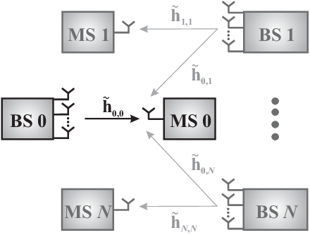
Let $\mathbf{\tilde{h}}_{k,\ell}\in\mathcal{C}^{n_{\rm T}}$ be the narrowband channel vector for the wireless link between MS $k$ and BS $\ell$ and also let $r_{k,\ell}$ denote the Euclidean distance between these nodes. The baseband received signal at MS $k$ can be mathematically expressed as

where the standard power-law pathloss model $l(r)=r^{-\alpha}$ with common pathloss exponent $\alpha>2$ for all links is assumed, $\mathcal{I}_{k}$ is the cumulative interference from all BSs except the associated BS $k$, which is given by

and $n_{k}\sim\mathcal{C}\mathcal{N}(0,\sigma^{2})$ denotes the additive white Gaussian noise (AWGN). Based on the considered system model described by (1) and (2), the signal-to-interference-plus-noise ratio (SINR) at MS $k$ can be computed as

The elements of each channel gain vector are assumed to be arbitrarily correlated and in particular, each $\mathbf{\tilde{h}}_{k,\ell}$ is modeled as $\mathbf{\tilde{h}}_{k,\ell}=\mathbf{R}^{1/2}\mathbf{h}_{k,\ell}$, where $\mathbf{h}_{k,\ell}\in\mathcal{C}^{n_{\rm T}}$ is a standard circularly-symmetric jointly-Gaussian random vector [18, Sec. 3.7] and $\mathbf{R}\triangleq\mathbb{E}\{\mathbf{\tilde{h}}_{k,\ell}\mathbf{\tilde{h}}_{k,\ell}^{\rm H}\}$ denotes the common covariance matrix of $\mathbf{\tilde{h}}_{k,\ell}$’s. In addition, we assume that $\mathbf{R}$ is real symmetric having ones in its main diagonal as well as that $\mathbf{\tilde{h}}_{k,\ell}$’s are independent across the different BSs and of both $r_{k,\ell}$’s and $n_{k}$’s.

In this paper, we assume that each BS $k$ knows perfectly $\mathbf{\tilde{h}}_{k,k}$ and treats interference as background noise. BSs do not cooperate [19] and each of them acts selfishly aiming at maximizing its own SNR. In order to accomplish that, each BS $k$ is assumed to perform channel-matched precoding, a.k.a. MRT. Hence, $\mathbf{f}_{k}$ at each BS $k$ is designed as [2, Sec. III]

In this section we present analytical expressions for the success probability and the area spectral efficiency of the considered downlink wireless network. The network performance is analyzed assuming a typical MS $0$ located at the origin. As a result of Palm probabilities (see [20] and references therein for details) and the stationarity of the PPP, the statistics of signal reception at the typical MS $0$ is seen by any MS in the considered wireless network.

In this section, numerically evaluated results for the performance expressions provided in Section III are presented and compared with equivalent results obtained by means of computer simulations. In particular, we numerically evaluate both the exact and the approximate expressions for $P_{\rm suc}$ given by (22) and (23), respectively, as well as those for ${\rm ASE}$ obtained from (24). Without loss of generality, in the performance evaluation results that follow, exponential correlation matrices have been considered and it has been assumed that $\alpha=3.5$, $r_{0,0}=1$ and $\sigma^{2}/{\rm P}=1$.

In Fig. 4, $P_{\rm suc}$ is plotted versus $\gamma_{\rm th}$ for $\lambda=10^{-4}$, $n_{\rm T}=2$ and $5$, and for $\rho=\{0.01,0.7,0.95\}$. As shown for all cases, the numerically evaluated results for the derived exact ($n_{\rm T}=2$) and the approximate ($n_{\rm T}=5$) $P_{\rm suc}$ match perfectly and are sufficiently close, respectively, with equivalent simulations. In addition, it is demonstrated that $P_{\rm suc}$ improves with decreasing $\gamma_{\rm th}$ and increasing $n_{\rm T}$. Interestingly, there exists a critical $\gamma_{\rm th}$ value, $\gamma_{\rm th}^{*}$, (crossing point in the figure) that increases with increasing $n_{\rm T}$ that determines the impact of $\rho$ on $P_{\rm suc}$. More specifically, for $\gamma_{\rm th}\leq\gamma_{\rm th}^{*}$, $P_{\rm suc}$ improves with decreasing $\rho$. However, when $\gamma_{\rm th}>\gamma_{\rm th}^{*}$, as $\rho$ decreases $P_{\rm suc}$ degrades.

By setting $\gamma_{\rm th}=3$ dB in Fig. 5, ${\rm ASE}$ is illustrated as a function of $\lambda$ for $n_{\rm T}=2$ and $\rho=\{0.01,0.7,0.95\}$. As shown in this figure, there exists a perfect match between the evaluated results for the derived exact ${\rm ASE}$ and equivalent simulations. In addition, the derived approximation appears to be a tight lower bound, which tightness increases as $\rho$ tends to either of its two extreme values (i.e. $\rho\rightarrow 0$ or $\rho\rightarrow 1$) as well as when $\lambda$ decreases. It is also demonstrated that ${\rm ASE}$ degrades with increasing $\rho$ and its maximum value happens for lower values of $\lambda$ as $\rho$ increases. The same performance metric over $\lambda$ is illustrated in Fig. 6 for cases where $\rho=0.7$ and $0.95$, $n_{\rm T}$ takes the values $5$ and $20$, and $\gamma_{\rm th}$ is increased to $5$ dB. In this figure, it is shown that ${\rm ASE}$ improves with increasing $n_{\rm T}$. In contrast to Fig. 5, as $\rho$ increases, ${\rm ASE}$ is shown to improve. Moreover, the maximum value for ${\rm ASE}$ happens for lower values of $\lambda$ as $\rho$ decreases. As also discussed in the description of Fig. 4, the latter behavior implies that, for the parameters’ setting in Figs. 5 and 6, $\rho$ has different impact on ${\rm ASE}$. Finally, it is noted that, as demonstrated in Fig. 6, the impact of $\rho$ on ${\rm ASE}$ increases with increasing $n_{\rm T}$.

In this paper, we have analyzed the performance of MRT in a wireless Poisson network assuming spatially arbitrarily correlated Rayleigh fading channels. Novel closed-form expressions for the distribution of the power of the interference resulting from the coexistence of one intended and one unintended MRT over the considered fading channels were first presented. Based on these expressions and using tools from stochastic geometry, we further derived closed-form expressions for the success probability and area spectral efficiency of the downlink network under investigation. Our theoretical analysis, which is corroborated with simulation results, shed light on how spatial fading correlation affects the network performance depending on the interplay between the density of BSs and the target SINR threshold. Interestingly, depending on the background noise level, spatial fading correlation may increase or decrease the network throughput, having a phase transition for a certain SINR threshold value.

References

- [1] J. Winters, “Optimum combining in digital mobile radio with cochannel interference,” IEEE Trans. Veh. Technol., vol. 2, no. 4, pp. 528–539, Aug. 1984.
- [2] T. K. Y. Lo, “Maximum ratio transmission,” IEEE Trans. Commun., vol. 47, no. 10, pp. 1458–1461, Oct. 1999.
- [3] Q. T. Zhang, “Maximal-ratio combining over Nakagami fading channels with an arbitrary branch covariance matrix,” IEEE Trans. Veh. Technol., vol. 48, no. 4, pp. 1141–1150, Jul. 1999.
- [4] P. Lombardo, G. Fedele, and M. M. Rao, “MRC performance for binary signals in Nakagami fading with general branch correlation,” IEEE Trans. Commun., vol. 47, no. 1, pp. 44–52, Jan. 1999.
- [5] S. L. Loyka, “Channel capacity of MIMO architecture using the exponential correlation matrix,” IEEE Trans. Commun., vol. 5, no. 9, pp. 369–371, Sep. 2001.
- [6] C.-N. Chuah, D. N. C. Tse, J. M. Kahn, and R. A. Valenzuela, “Capacity scaling in MIMO wireless systems under correlated fading,” IEEE Trans. Inf. Theory, vol. 48, no. 3, pp. 637–650, Mar. 2002.
- [7] A. M. Tulino, A. Lozano, and S. Verdú, “Impact of antenna correlation on the capacity of multiantenna channels,” IEEE Trans. Inf. Theory, vol. 51, no. 7, pp. 2491–2509, Jul. 2005.
- [8] G. C. Alexandropoulos, N. C. Sagias, F. I. Lazarakis, and K. Berberidis, “New results for the multivariate Nakagami- fading model with arbitrary correlation matrix and applications,” IEEE Trans. Wireless Commun., vol. 8, no. 1, pp. 245–255, Jan. 2009.
- [9] D. Park and S. Park, “Effect of transmit antenna correlation on multiuser diversity,” in Proc. IEEE ISIT, Adelaide, Australia, 4-9 Sep. 2005, pp. 1421–1425.
- [10] H. Kim, W. Choi, and H. Park, “Effects of antenna correlation on spatial diversity and multiuser diversity,” in Proc. IEEE WCNC, Las Vegas, USA, 31 Mar.-3 Apr. 2008, pp. 65–69.
- [11] A. Hunter, J. G. Andrews, and S. Weber, “Transmission capacity of ad hoc networks with spatial diversity,” IEEE Trans. Wireless Commun., vol. 7, no. 12, pp. 5058–5071, Dec. 2008.
- [12] N. Jindal, J. G. Andrews, and S. Weber, “Rethinking MIMO for wireless networks: Linear throughput increases with multiple receive antennas,” in Proc. IEEE ICC, Dresden, Germany, 14-18 Jun. 2009, pp. 1–6.
- [13] O. B. S. Ali, C. Cardinal, and F. Gagnon, “Performance of optimum combining in a Poisson field of interferers and Rayleigh fading channels,” IEEE Trans. Wireless Commun., vol. 9, no. 8, pp. 2461–2467, Aug. 2010.
- [14] R. H. Y. Louie, M. R. McKay, and I. B. Collings, “Open-loop spatial multiplexing and diversity communications in ad hoc networks,” IEEE Trans. Inf. Theory, vol. 57, no. 1, pp. 317–344, Jan. 2011.
- [15] M. Haenggi, “Diversity loss due to interference correlation,” IEEE Commun. Lett., vol. 16, no. 10, pp. 1600–1603, Oct. 2012.
- [16] R. Tanbourgi, H. S. Dhillon, J. G. Andrews, and F. K. Jondral, “Effect of spatial interference correlation on the performance of maximum ratio combining,” IEEE Trans. Wireless Commun., vol. 13, no. 6, pp. 3307–3316, Jun. 2014.
- [17] I. S. Gradshteyn and I. M. Ryzhik, Table of Integrals, Series, and Products, 6th ed. New York: Academic, 2000.
- [18] R. G. Gallager, Stochastic Processes: Theory for Applications. Cambridge: Cambridge University Press, 2013.
- [19] A. Lozano, R. W. Heath, and J. G. Andrews, “Fundamental limits of cooperation,” IEEE Trans. Inf. Theory, vol. 59, no. 9, pp. 5213–5226, Mar. 2013.
- [20] J. G. Andrews, F. Baccelli, and R. K. Ganti, “A tractable approach to coverage and rate in cellular networks,” IEEE Trans. Commun., vol. 59, no. 11, pp. 3122–3134, Nov. 2011.
- [21] A. Shah and A. M. Haimovich, “Performance analysis of maximal ratio combining and comparison with optimum combining for mobile radio communications with cochannel interference,” IEEE Trans. Veh. Technol., vol. 49, no. 4, pp. 1454–1463, Jul. 2000.
- [22] G. C. Alexandropoulos, “On the distribution of the Rayleigh quotient and applications in the performance analysis of wireless communication systems,” under preparation, 2015.