Isospin splittings of meson and baryon masses from three-flavor lattice QCD + QED

Isospin breaking effects are crucial for the existence of our Universe. Our Universe would not exist in the present form if the $n-p$ mass difference would only be slightly different. If it would be larger than the binding energy of the deuteron, no fusion would take place. If it would be a little smaller, all hydrogen would have been burned to helium. Isospin breaking in hadron masses has two sources, the mass difference of up and down quarks, and electromagnetic interactions. Both effects are of the same order of magnitude and cannot be separated unambiguously due to the nonperturbative nature of the strong interactions. This makes a direct calculation from QCD + QED necessary [1, 2, 3]. While substantial progress has been made, [3] is the only other published work to report simulations with fully dynamical QCD + QED.

In [4, 5] we have outlined a program to systematically investigate the pattern of flavor symmetry breaking in three-flavor lattice QCD for Wilson-type fermions. Our strategy was to start from the SU(3) symmetric point with all three quark masses equal, $m_{u}=m_{d}=m_{s}$, and extrapolate towards the physical point keeping the average sea quark mass $\bar{m}=\left(m_{u}+m_{d}+m_{s}\right)/3$ constant. For this trajectory to reach the physical quark masses, $\bar{m}$ is tuned to the physical value of the average pseudoscalar meson mass $X_{\pi}^{2}=\left(M_{K^{0}}^{2}+M_{K^{+}}^{2}+2M_{\pi^{0}}^{2}-M_{\pi^{+}}^{2}\right)/3$. We denote the distance from $\bar{m}$ by $\delta m_{q}=m_{q}-\bar{m}\ (q=u,d,s)\,.$ This implies $\delta m_{u}+\delta m_{d}+\delta m_{s}=0$ on our quark mass trajectory. To describe how physical quantities depend on the quark masses, we Taylor expand about the symmetric point [5]. This results in polynomials in $\bar{m}$ and $\delta m_{q}$, which we classify into representations of the SU(3) and $\mathrm{S_{3}}$ flavor groups. As we keep $\bar{m}$ constant and change only the octet part of the mass matrix, to first order in $\delta m_{q}$ flavor symmetry is broken by an SU(3) octet, leading to Gell-Mann–Okubo mass relations. We follow a similar approach here with QED added [2].

The symmetry of the electromagnetic current is similar to the symmetry of the quark mass matrix. The simplifications that come from $\delta m_{u}+\delta m_{d}+\delta m_{s}=0$ in the mass case are analogous to the simplifications we get from the identity $e_{u}+e_{d}+e_{s}=0$. A difference between quark mass and electromagnetic expansions is that in the mass expansion we can have both odd and even powers of $\delta m_{q}$, whereas only even powers of the quark charges $e_{q}$ are allowed. We consider contributions of $O(e_{q}^{2})$ only. Hence, QED corrections can be simply read off from the mass expansion presented in [5], dropping the linear terms and changing masses to charges.

For the masses of octet mesons with the flavor structure $a\bar{b}$, and all annihilation diagrams turned off, we find to leading order in $\alpha_{\rm EM}$

up to corrections of $O(\delta m_{q}^{2})$. Several of the coefficients in (1) can be matched up with different classes of Feynman diagrams shown in Fig. 1. The first diagram, with both ends of the photon attached to the same valence quark, contributes to $(\beta_{1}^{\rm EM}+\beta_{2}^{\rm EM})$. The second diagram, with the photon crossing between the valence lines, contributes to $\beta_{2}^{\rm EM}$. The last diagram, with the photon being attached to the sea quarks, is an example of a diagram contributing to $\beta_{0}^{\rm EM}$. It would be missed out if the electromagnetic field was quenched instead of dynamical. Similar assignments hold for the mixed (charge squared times mass) terms. For a single choice of sea quark masses, the $\beta_{0}^{\rm EM}$ and $\gamma_{4}^{\rm EM}$ terms can be absorbed into the constant $M_{0}^{2}$ and the $\alpha$ term. However, for a combined fit of both QCD and QCD + QED data we will need these coefficients. More details can be found in [6]. Similarly, for octet baryons with the flavor structure $aab$ we find to leading order in $\alpha_{\rm EM}$

up to corrections of $O(\delta m_{q}^{2})$. This excludes the case of baryons with three different quarks, as in the $\Sigma^{0}-\Lambda$ system [7]. Again, the $\beta_{0}^{\rm EM}$ term can be absorbed into the mass term $M_{0}^{2}$. The coefficients $\beta_{1}^{\rm EM}$, $\beta_{2}^{\rm EM}$ and $\beta_{3}^{\rm EM}$ can be matched up with distinct classes of Feynman diagrams similar to the ones in Fig. 1.

Our goal is to compute the mass splittings of pseudoscalar mesons and octet baryons at the physical point for QCD + QED. This amounts to determining the coefficients $\alpha$, $\beta^{\rm EM}$ and $\gamma^{\rm EM}$ in (1) and (2). It greatly helps to vary valence and sea quark masses independently [5], which is referred to as partial quenching (PQ). In this case the sea quark masses remain constrained by $\bar{m}=\mbox{constant}$, while the valence quark masses $\mu_{u}$, $\mu_{d}$ and $\mu_{s}$ are unconstrained. Defining $\delta\mu_{q}=\mu_{q}-\bar{m}$, the resulting modification of Eq. (1) to PQ octet mesons is

For octet baryons Eq. (2) becomes

The coefficients $\alpha$, $\beta^{\rm EM}$ and $\gamma^{\rm EM}$ in (3) and (4) are identical to those in (1) and (2). This is to say that hadron mass splittings are unaffected by PQ at this order, as PQ moves (e.g.) all octet mesons and baryons by the same amount. We would have to expand to cubic terms to see PQ errors in the splittings [5]. Hence, PQ calculations offer a computationally cheaper way of obtaining them.

In QCD + QED there is some ambiguity in the definition of the symmetric point. The definition we have chosen is that the electrically neutral pseudoscalar mesons have the same masses, $M^{2}(u\bar{u})=M^{2}(d\bar{d})=M^{2}(s\bar{s})=M^{2}(d\bar{s})=M^{2}(s\bar{d})=M^{2}(n\bar{n})\,,$ where $n$ is a fictitious electrically neutral quark. As annihilation diagrams are neglected, different neutral mesons do not mix. We denote the Wilson hopping parameter $\kappa$ (introduced in (7) below) marking the symmetric point by $\bar{\kappa}_{q}$. We then have $\delta m_{q}=(m_{q}-\bar{m})=1/2\kappa_{q}^{\rm sea}-1/2\bar{\kappa}_{q}$ and $\delta\mu_{q}=(\mu_{q}-\bar{m})=1/2\kappa_{q}^{\rm val}-1/2\bar{\kappa}_{q}$, setting the lattice spacing $a=1$. It should be noted that even when all three quark masses are equal we do not have full SU(3) symmetry. Because of their different charges, the $u$ quark is always distinguishable from the $d$ and $s$ quark.

The action we are using is

Here $S_{G}$ is the tree-level Symanzik improved SU(3) gauge action with gauge coupling $\beta=6/g^{2}$, and $S_{A}$ is the noncompact U(1) gauge action [8, 9] of the photon,

We employ the nonperturbatively ${\cal O}(a)$ improved SLiNC fermion action [10] for each quark flavor,

This action features single iterated mildly stout smeared QCD links with $\alpha=0.1$ [5] and unsmeared QED links in the hopping terms, while the clover term contains unsmeared QCD links only. We keep the action deliberately local, as excessive smearing will lead to large autocorrelation times. Stout smearing is analytic, so a derivative can be taken, which makes the HMC force well defined. The clover coefficient has been computed nonperturbatively in QCD [10]. We presently neglect electromagnetic modifications to the clover term. This will leave us with corrections of $O(\alpha_{\rm EM}\,e_{q}^{2}\,a)$, which turn out to be no larger than the $O(a^{2})$ corrections from QCD in our simulations. We check this later by comparing neutral meson masses with different quark charges $e_{q}$ (Fig. 3). Adding an electromagnetic clover term with $c_{SW}^{\rm EM}=1$ would leave us with corrections of $O(\alpha_{\rm EM}\,e_{q}^{2}\,g^{2}a)$ (to this order in $\alpha_{\rm EM}$), which is not a significant improvement, if at all. Simulations are performed using the HMC and RHMC [11] algorithms. The gluon field and the EM field are updated sequentially.

In this study, we limit our calculations to a single value of the strong coupling constant (lattice spacing) $\beta=5.50$, where we have our largest sample of dynamical QCD configurations [12]. Furthermore, we restrict ourselves to simulations at the symmetric point, $\delta m_{u}=\delta m_{d}=\delta m_{s}=0$, which we define as $X_{\pi}^{2}/X_{N}^{2}=0.126$, where $X_{N}^{2}=\left(M_{n}^{2}+M_{p}^{2}+M_{\Sigma^{-}}^{2}+M_{\Sigma^{+}}^{2}+M_{\Xi^{-}}^{2}+M_{\Xi^{0}}^{2}\right)/6$. We may use either $X_{\pi}$ or $X_{N}$ to set the scale [5]. After several tuning runs carried out on $24^{3}\times 48$ lattices we arrived at the $\kappa$ values $\bar{\kappa}_{u}=0.124362\,,\ \bar{\kappa}_{d}=\bar{\kappa}_{s}=0.121713$. At these $\kappa$ values, we study three different volumes, $24^{3}\times 48$, $32^{3}\times 64$ and $48^{3}\times 96$, with $O(2000)$ to $O(500)$ trajectories. We like to add that simulations at the symmetric point already catch the essential features of the physical QCD + QED vacuum, as flavor singlet quantities vary slowly along the $\bar{m}=\mbox{constant}$ trajectory [5].

On these ensembles we have computed PQ pseudoscalar meson and octet baryon masses for a variety of quark masses ranging from $m_{PS}/m_{N}=0.22$ to $0.5$, with $e_{q}=-1/3,0$ and $+2/3$. This leads to about 40 pseudoscalar masses and 70 baryon masses per ensemble. The baryons include several artificial states containing the fictitious $n$ quark and charge 2 baryons with flavor structure $uuu^{\prime}$.

The action (5) is invariant under $\mathrm{U(1)}$ gauge transformations

However, this is not the case for propagators of charged particles, which demands fixing the gauge, as in perturbation theory. We choose the Landau gauge, which is defined by the condition $\bar{\Delta}_{\mu}A_{\mu}(x)=0$, where $\Delta_{\mu}$ ($\bar{\Delta}_{\mu}$) is the forward (backward) lattice derivative. The Landau gauge does not eliminate all gauge degrees of freedom, but allows for shifts $\Delta_{\mu}\alpha(x)$ of the photon field with $\Delta^{2}\alpha(x)=0$, where $\Delta^{2}=\Delta_{\mu}\bar{\Delta}_{\mu}$ [9]. To maintain (anti-)periodicity of the quark fields, $\alpha(x)$ must be periodic up to a transformation of the form

where $L_{\mu}$ is the extent of the lattice in $\mu$ direction. This gauge field redundancy can be eliminated by adding multiples of $2\pi/e_{q}L_{\mu}$ to $A_{\mu}(x)$, such that

Taking $e_{q}=-1/3$ in (9) serves both charges. The advantage of this procedure is that it leaves the fermion determinant and Polyakov loops for all quark flavors unchanged. In other popular gauges [3] this is not the case, but results in a permanent Polyakov loop $\Pi_{x_{\nu},\nu\neq\mu}\,L_{\mu}^{\rm EM}(x_{\nu})=1$, which we would not know how to correct for in a simple manner.

The constant background field can be factored out from the link matrices, configuration by configuration, and absorbed into the quark momenta by straightforward algebra.¹¹ 1 Note that the transformation $\displaystyle q(x)\rightarrow e^{i\Delta x}\,q(x)\,,\;\bar{q}(x)\rightarrow\bar{q}(x)\,e^{-i\Delta x}$ amounts to a shift of quark momenta $\displaystyle p\rightarrow p+\Delta$. This leaves us with photon propagators that are devoid of zero modes. In the presence of a constant background field $B_{\mu}$ the correlator of a single hadron $H$ thus becomes [9]

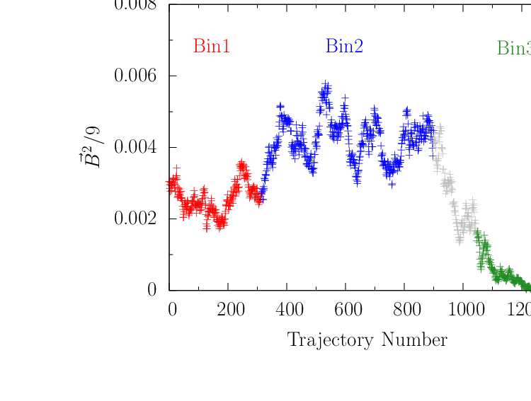
where $M_{H}$, $\vec{p}$ and $e_{H}$ are mass, three-momentum and electric charge of the hadron, respectively. This amounts to a shift of the rest energy of the charged hadrons, $M_{H}\rightarrow\sqrt{M_{H}^{2}+e_{H}^{2}\,\vec{B}^{2}}\simeq M_{H}+e_{H}^{2}\,\vec{B}^{2}/2M_{H}$. We determine the ensemble average of $\vec{B^{2}}$ directly on each of our three volumes. The result is $0.024$, $0.0079$ and $0.000095$ for the smallest to largest volumes, respectively. To extract masses, we remove the influence of the background field effect by subtracting the associated kinetic energy from the ensemble averaged lattice energy. To demonstrate the validity of this procedure, we have divided a subset of our $24^{3}\times 48$ ensemble into three bins of approximately constant background field in Fig. 2 and plot the corresponding lattice energies for each of these bins against the corresponding $\vec{B^{2}}$. It shows that both the energies of the individual bins as well as the ensemble averaged energy fall on a single straight line, in line with our subtraction method. On the $48^{3}\times 96$ lattice the effect of the background field is comparable to our statistical precision. With the zero modes removed, we then can employ established methods, such as [13], to correct for the remaining electromagnetic finite size effects associated with the long-range tail of the photon field. Any residual effect of the background field will only act to modify the recoil energy of any charged hadron propagator within loops.

Our strategy is to simulate at an artificial coupling $e^{2}=1.25$, and then interpolate between this point and pure QCD to the physical fine structure constant $\alpha_{\rm EM}=1/137$. This value is chosen so that electromagnetic effects can be easily seen, but is still small enough that they scale linearly in $e^{2}$ and we do not need to consider higher order terms. Most importantly, $Z_{3}=0.94(3)$, obtained from the vacuum polarization. Furthermore, in Figs. 4 and 5 of [6] we have plotted $1/\kappa_{q}^{c}\,,\,1/\bar{\kappa}_{q}$ and the bare quark mass at the symmetric point, $1/2\bar{\kappa}_{q}-1/2\kappa_{q}^{c}$, against $e_{q}^{2}$ for $e_{q}=-1/3,0$ and $2/3$ and found that all three quantities lie on a straight line. In addition, we find that the coefficients $\alpha$ and $\alpha_{1},\,\alpha_{2}$ in (3) and (4) agree to a good precision with the corresponding numbers in pure QCD [5]. This rules out significant higher order corrections in $e^{2}$.

After the initial small volume tuning runs, it turns out that the chosen $\kappa$ values do not quite satisfy our constraint of equal neutral pseudoscalar meson masses. A more accurate estimate can be determined from a fit to the pseudoscalar meson masses. On the $48^{3}\times 96$ lattice we obtain

which is only a small displacement from the underlying simulation kappas. We shall expand about these $\kappa$ values in our subsequent fits.

In contrast to QCD, equal meson masses at the symmetric point no longer mean equal bare quark masses. We renormalize the quark masses to remove this defect. We do so by absorbing the QED terms of the neutral pseudoscalar mesons into the quark self-energies. On our symmetric background, $\delta m_{u}=\delta m_{d}=\delta m_{s}=0$, this is achieved by replacing $\delta\mu_{q}$ by the ‘Dashen’ scheme mass [6]

Substituting (12) into (3), and absorbing $\beta_{0}^{\rm EM}$ into $M_{0}^{2}$ and $\gamma_{4}^{\rm EM}$ into $\alpha$, we obtain in the ‘Dashen’ scheme

Note that since we choose the neutral pseudoscalar mesons to have the same mass, $\beta_{1}^{\rm EM}=0$ by definition. We define the critical point, $\kappa_{q}^{c}$ for each flavor, to be the point where the masses of the neutral pseudoscalar mesons vanish. It is then easily seen that the ‘Dashen’ scheme quark masses are all equal at the symmetric point, $\bar{\mu}_{q}^{D}=M_{0}^{2}/2\alpha$, $q=u,d,s$ and $n$, see [6] for further details. It follows that the total electromagnetic contributions to the neutral pseudoscalar meson masses, $M_{\pi^{0}}$ and $M_{K^{0}}$, are zero. In Fig. 3 we show the neutral meson masses $M^{2}(a\bar{a})$ against $\delta\mu_{a}^{D}$. It is striking to see that the data fall perfectly on a straight line, which strongly supports our group-theoretical classification of SU(3) flavor symmetry breaking as well as octet (Gell-Mann–Okubo) type mass splitting. $O(\alpha_{\rm EM}\,e_{a}^{2}\,a)$ corrections would result in deviations from the straight line proportional to $e_{a}^{2}$, for which we see no evidence. To be consistent, we also expand the baryon masses in terms of the ‘Dashen’ masses,

In Fig. 4 we show the charge $e_{N}=+1$ baryon masses $M^{2}(aab)$ against $2\delta\mu^{D}_{a}+\delta\mu^{D}_{b}$. Again, the data fall perfectly on a straight line, in accord with our flavor expansions.

For the total contribution of QCD + QED it does not matter which scheme we use to define the quark masses, but for the individual contributions of QCD and QED it will make a difference. The fits of (13) and (14) to the lattice data are quite robust, giving $\chi^{2}/\mbox{dof}=0.7-1.2$. To obtain physical numbers, we extrapolate the coefficients $\beta_{i}^{\rm EM}$ and $\gamma_{i}^{\rm EM}$ to $\alpha_{\rm EM}=1/137$ by scaling them with a factor $\sim 10/137$. In our extrapolation to the physical point we keep the sum of the quark masses constant. We choose $M_{\pi^{0}}^{2}$ and $M_{K^{0}}^{2}-M_{K^{+}}^{2}+M_{\pi^{+}}^{2}-M_{\pi^{0}}^{2}$ to determine the physical $\kappa$ values. In Fig. 5 we show the result of the fit to the meson and baryon masses on the $48^{3}\times 96$ lattice. We obtain $X_{\pi}^{2}/X_{N}^{2}=0.128(3)$, which is to be compared with the physical value, $0.126$. This tells us that we have hit the symmetric point with remarkable precision. Using $X_{\pi}$ to set the scale, the lattice spacing turns out to be $a=0.068(2)\,\mbox{fm}$. The figure also indicates that the baryon masses extrapolate nicely to their experimental values, leaving little room for quadratic terms. Similarly good results are found on the $32^{3}\times 64$ lattice. Having found the $\kappa$ values of the physical point and the point where the ‘Dashen’ scheme masses vanish (the critical point), we can determine the quark masses. For the quark mass ratios we find on the $48^{3}\times 96$ lattice in the ‘Dashen’ scheme

In [6] we have shown how to switch between the ‘Dashen’ and $\overline{\rm MS}$ schemes. Applying this, we find the ratio $m_{u}/m_{d}$ in the $\overline{\rm MS}$ scheme at $\mu^{2}=4\,{\rm GeV}^{2}$ decreases by less than a percent, whereas $m_{s}/m_{d}$ remains a renormalization group invariant, even in the presence of QED. Hence Eq. (15) represents our results in the $\overline{\rm MS}$ scheme at $\mu^{2}=4\,{\rm GeV}^{2}$.

In this Letter we are primarily interested in the isospin splittings of pseudoscalar meson and octet baryon masses. To get to our final numbers, we need to correct for finite size effects first. From QED we expect power-law corrections, due to the photon being massless, in addition to exponential corrections from QCD. We correct for QCD finite size effects by using the results of [14, 15], adapted to three flavors of PQ quarks. In case of the nucleon the corrections amount to approximately $1\%$ on the $48^{3}\times 96$ lattice and to $5\%$ on the $32^{3}\times 64$ lattice. Having successfully removed the zero modes, we can correct for the remaining QED effects by employing the mass shift formulae of effective field theory (EFT) [13]. We test this in Fig. 6, where we compare the QED contribution to the $p-n$ mass splitting, $(M_{p}-M_{n})_{\rm QED}$, with the prediction of [13] on our two largest volumes. We find good agreement between the data and the analytic expression, indicating that QED finite size effects are well accounted for by EFT. In Fig. 7 we present our QCD + QED results for the isospin splittings of mesons and baryons as a function of lattice size. The curves represent the predictions of [13]. They have been drawn through the points on the $48^{3}\times 96$ lattice. We find good agreement between the curves and our points on the two largest lattices, while the data on the $24^{3}\times 48$ lattice (with $L\approx 1.6\,\mbox{fm}$) appear to lie outside the range of validity of the expansion. We consider the extrapolation of the $48^{3}\times 96$ lattice points to $a/L=0$ by [13] our best estimate of the infinite volume result. We compare this result with a fit to the points on the two largest lattices. The differences are taken as an estimate of systematic error. In Table 1 we list our final results for the mass splittings in the infinite volume, for the total and the QED contribution separately. Following [6], we find the QED contributions in the ‘Dashen’ scheme and the $\overline{\rm MS}$ scheme at $\mu^{2}=4\,{\rm GeV}^{2}$ to differ by less than a percent. As a result, the QED contributions in Table 1 also represent our results in the $\overline{\rm MS}$ scheme at $\mu^{2}=4\,{\rm GeV}^{2}$. The traditional way of expressing the electromagnetic contributions is through $\Delta_{\pi}=M_{\pi^{+}}^{2}-M_{\pi^{0}}^{2}$ and the $\epsilon$ parameter,

On the $48^{3}\times 96$ lattice we find $\epsilon=0.49(5)$, which translated to $\overline{\rm MS}$ gives [6]

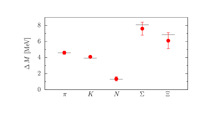
This result is well within the range quoted by FLAG [17], albeit with significantly reduced uncertainty. We now can compare the baryon mass splittings of this calculation with our recent results from pure QCD [16]. The QCD numbers are quoted in the fourth column of Table 1. They have been brought in line with our new value of $\epsilon$ (17). Both sets of results are found to be largely consistent. It is worth emphasizing that the QED and pure QCD contributions to the nucleon mass splitting sum up nicely to the total QCD + QED contribution, which is encouraging. Finally, in the last column of Table 1 we quote the experimental mass splittings. We observe good agreement for both octet pseudoscalar mesons and octet baryons. Since we have not yet computed the QCD contribution to the $\pi^{0}$ mass from $\pi^{0}$–$\eta$ mixing, arising from quark-line disconnected diagrams, we only quote the QED contribution to the $M_{\pi^{+}}-M_{\pi^{0}}$ mass difference. It is worth noting that phenomenological estimates for the disconnected contribution are of the order of 0.1 MeV [18], which is within the precision of our present calculation. Figure 8 summarizes our results.

Both the total QCD + QED mass splittings as well as the QED contributions satisfy the Coleman-Glashow relation [19] by construction. So do the experimental values, which once again supports our group-theoretical approach and truncation (14). The QED contribution to the $n-p$ mass splitting in the ‘Dashen’ and $\overline{\rm MS}$ schemes turns out to be somewhat larger (in absolute terms) than the numbers derived from the Cottingham formula [20]. It should be noted though that the individual estimates [20] cover a wide range of values. To accommodate the lower numbers from the Cottingham formula, the result of pure QCD [16] (fourth column of Table 1) would have to be smaller by a factor up to two as well. Our QED result is also larger than the recently reported lattice number in [3]. In our approach the QED and QCD separation is defined within the meson sector. In contrast, [3] chose the QED part of the $\Sigma^{+}-\Sigma^{-}$ mass difference to be zero, for which we identify a clear nonzero signal. This would be the case if $(2/3)\,\beta_{1}^{\rm EM}+\beta_{2}^{\rm EM}+(1/3)\,\beta_{3}^{\rm EM}=0$ in our mass expansion (14). A fit to our data with this constraint gives $(M_{n}-M_{p})_{\rm QED}=-1.71(28)(10)\,\mbox{MeV}$ in the ‘Dashen’ scheme. While this result is largely compatible with the analysis of Walker-Loud, Carlson and Miller [20], $(M_{n}-M_{p})_{\rm QED}=-1.30(50)\,\mbox{MeV}$, it illustrates quite clearly that the QED part of the $n-p$ mass difference depends sensitively on how electromagnetic and strong contributions are separated. While our results do not support higher order terms in the quark mass expansion, it may be possible that one source of the discrepancy could be related to nonlinearities in the chiral behavior of the electromagnetic self energy [21] that are not being captured by the Taylor expansion.

As discussed in the introduction, the existence of the Universe as we know it is highly sensitive to the magnitude of the $n-p$ mass difference. Having an analytic expression for the mass of neutron and proton, Eq. (14), we can express the allowed region in terms of the fundamental parameters $m_{u},m_{d}$ and $\alpha_{\rm EM}$, as shown in Fig. 9. Not shown are the bounds on $\alpha_{\rm EM}$ from the stability of atoms [22]. It turns out that both $\alpha_{\rm EM}$ and the ratio of light quark masses $m_{u}/m_{d}$ are finely tuned. At the physical fine structure constant the ratio is restricted to a narrow region around $m_{u}/m_{d}=0.5$.

We have outlined a program to systematically investigate the flavor structure of hadrons in a full QCD + QED lattice simulation. By treating the valence quark masses differently to those in the sea allows for a range of valence quark masses and charges to be explored and significantly enhances our ability to accurately constrain the fit parameters in our flavor-breaking expansions. As a result, we have successfully computed the isospin splittings of pseudoscalar meson and octet baryon masses. By using our recently introduced ‘Dashen’ scheme as an intermediate step [6], we are able to quote the first lattice results for the QED contribution to the $n-p$ mass splitting in the ${\overline{\rm MS}}$ scheme.

The calculations have been done at lattice spacing $a=0.068\,\mbox{fm}$. At this lattice spacing discretization errors are expected to be less than $2\%$ [12], which are well below our present statistical and systematic errors. To reduce the errors and gain full control over the infinite volume extrapolation, simulations on $64^{3}\times 128$ lattices and larger will have to be done. To further constrain our fits, and test for potential $\delta m_{q}$ effects, we have started dynamical $1+1+1$ flavor simulations along the $\bar{m}=\mbox{const}$ line, with $\delta m_{u}\neq\delta m_{d}\neq\delta m_{s}\neq 0$ and sea quark masses approaching the physical point. Finally, future simulations will also naturally be required on lattices with different lattice spacings to allow for a continuum extrapolation.

This work has been partly supported by DFG through grant SCHI 422/10-1 (HP) and the Australian Research Council through grants DP140103067 (RDY and JMZ), FT120100821 (RDY) and FT100100005 (JMZ). The numerical calculations were carried out on the BlueGeneQs at FZ Jülich and EPCC Edinburgh (using DIRAC 2), the Cray XC30 at HLRN (Berlin and Hannover) and on the NCI National Facility (Canberra).

References

- [1] For recent work see: T. Blum et al., Phys. Rev. D 82 (2010) 094508 [arXiv:1006.1311 [hep-lat]], S. Aoki et al., Phys. Rev. D 86 (2012) 034507 [arXiv:1205.2961 [hep-lat]], Sz. Borsanyi et al., Phys. Rev. Lett. 111 (2013) 25, 252001 [arXiv:1306.2287 [hep-lat]], G. M. de Divitiis et al. Phys. Rev. D 87 (2013) 11, 114505 [arXiv:1303.4896 [hep-lat]], R. Zhou and S. Gottlieb, PoS LATTICE 2014 (2014) 024 [arXiv:1411.4115 [hep-lat]], M. G. Endres, A. Shindler, B. C. Tiburzi and A. Walker-Loud, arXiv:1507.08916 [hep-lat].
- [2] R. Horsley et al., PoS Lattice 2013 (2014) 499 [arXiv:1311.4554 [hep-lat]].
- [3] S. Borsanyi et al., Science 347 (2015) 1452 [arXiv:1406.4088 [hep-lat]].
- [4] W. Bietenholz et al., Phys. Lett. B 690 (2010) 436 [arXiv:1003.1114 [hep-lat]].
- [5] W. Bietenholz et al., Phys. Rev. D 84 (2011) 054509 [arXiv:1102.5300 [hep-lat]].
- [6] R. Horsley et al., JHEP 1604 (2016) 093 [arXiv:1509.00799 [hep-lat]].
- [7] R. Horsley et al., Phys. Rev. D 91 (2015) 7, 074512 [arXiv:1411.7665 [hep-lat]].
- [8] M. Göckeler et al., Nucl. Phys. B 334 (1990) 527.
- [9] M. Göckeler, R. Horsley, P. E. L. Rakow, G. Schierholz and R. Sommer, Nucl. Phys. B 371 (1992) 713.
- [10] N. Cundy et al., Phys. Rev. D 79 (2009) 094507 [arXiv:0901.3302 [hep-lat]].
- [11] M. A. Clark and A. D. Kennedy, Phys. Rev. Lett. 98 (2007) 051601 [hep-lat/0608015].
- [12] V. G. Bornyakov et al., arXiv:1508.05916 [hep-lat].
- [13] Z. Davoudi and M. J. Savage, Phys. Rev. D 90 (2014) 054503 [arXiv:1402.6741 [hep-lat]].
- [14] A. Ali Khan et al., Nucl. Phys. B 689 (2004) 175 [hep-lat/0312030].
- [15] G. Colangelo, S. Dürr and C. Haefeli, Nucl. Phys. B 721 (2005) 136 [hep-lat/0503014].
- [16] R. Horsley et al., Phys. Rev. D 86 (2012) 114511 [arXiv:1206.3156 [hep-lat]].
- [17] S. Aoki et al., Eur. Phys. J. C 74 (2014) 2890 [arXiv:1310.8555 [hep-lat]].
- [18] J. Gasser and H. Leutwyler, Phys. Rept. 87 (1982) 77.
- [19] S. R. Coleman and S. L. Glashow, Phys. Rev. Lett. 6 (1961) 423.
- [20] J. Gasser and H. Leutwyler, Nucl. Phys. B 94 (1975) 269, A. Walker-Loud, C. E. Carlson and G. A. Miller, Phys. Rev. Lett. 108 (2012) 232301 [arXiv:1203.0254 [nucl-th]], F. B. Erben, P. E. Shanahan, A. W. Thomas and R. D. Young, Phys. Rev. C 90 (2014) 6, 065205 [arXiv:1408.6628 [nucl-th]], J. Gasser, M. Hoferichter, H. Leutwyler and A. Rusetsky, Eur. Phys. J. C 75 (2015) 8, 375 [arXiv:1506.06747 [hep-ph]].
- [21] A. W. Thomas, X. G. Wang and R. D. Young, Phys. Rev. C 91 (2015) 1, 015209 (2015) [arXiv:1406.4579 [nucl-th]].
- [22] See, for example, E. H. Lieb and W. E. Thirring, The stability of matter: From atoms to stars. Selecta of Elliott H. Lieb, Berlin, Germany: Springer (2001)