Randomness determines practical security of BB84 quantum key distribution

Quantum key distribution (QKD) [1] is the art of sharing secret keys between two remote parties Alice and Bob, unconditional security of which is based on the fundamental laws of quantum mechanics. The detailed security analysis has been proved by applying the entanglement distillation and purification (EDP) technology [2, 3] and the von Neumann entropy theory [4, 5, 6] respectively. However, unconditional security of the QKD protocol has an important assumption, which requires Alice and Bob have random numbers to control the classical bit encoding and measurement bases selection, and it can be easily proved that security of the final key can’t be guaranteed if input random numbers are controlled or known by the eavesdropper Eve. In recent years, practical QKD system was attacked by considering the imperfect state preparation and measurement respectively [7]. More generally, the practical attacking scheme can be divided into three different types. The first type is considering the Trojan horse attack [8], where the signal state combining with the trojan horse state can be assumed to be high dimensional state modulation. Note that Eve can measure one dimension of the modulated high dimensional state to get all of the secret key information without being discovered, thus Alice and Bob should apply the dimension filter (such as wavelength filter) to avoid this attack.

The second type is the strong randomness attack, which considers some of the input random numbers are totally controlled by the eavesdropper Eve. Such as the multi photon state can be attacked by applying the photon number splitting (PNS) attack [9, 10], where the multi photon encoding quantum states can be assumed to be known by Eve. Another example is the detector blinding attack [11, 12], where Eve can easily mount the man-in-the-middle (MITM) attack by converting the avalanche photodiodes (APDs) into linear mode. The detectors have the count iff Bob’s bases selection is equal to Eve, which means that the bases selection in Bob’s side are controlled by Eve. Recently we propose the probabilistic blinding attack model [13], where Eve partly applies the blinding attack to avoid being catched by detecting the current parameter. In the strong randomness attack model, the final secret key rate should delete all of the counting events known by Eve. The GLLP [14] secret key rate and the decoy state method [15, 16, 17] can be assumed to delete all of the multi photon pulse counting result, and only the single photon counting event can generate the final secret key. While the probabilistic blinding attack can be assumed to delete all of the blinding counting results, and only the non-blinding counting event can generate the final secret key. In the strong randomness attack model, the previous secret key rate [18] formula can be modified to

where $p$ is the probability of valid counting result, which can’t be controlled by Eve. $a$ is Alice’s measurement outcomes, $E$ is Eve’s auxiliary quantum system, $S(a|E)=S(a,E)-S(E)$ is the conditional von Neumann entropy, which demonstrates Eve’s uncertainty about Alice’s key bit $a$. $e$ is the practical bit error rate, $h(e)=-elog_{2}e-(1-e)log_{2}(1-e)$ is the classical Shannon entropy function, $f\geq 1$ is the error correction efficiency. If we consider the PNS attack, $p$ can be illustrated by the single photon counting rate, $S(a|E)$ can be estimated by the single photon error rate.

The third type is the weak randomness attack, which considers input random numbers are partly controlled by Eve [19]. Such as the wavelength dependence about the beam splitter will introduce the wavelength attack [20], where Eve can apply different wavelengths to control Bob’s bases selection. Since the practical beam splitter and different wavelengths may only have partial correlation, which means the beam splitter coupling ratio can’t reach $0$ and $1$ with two different bases, thus Eve can only partly control bases selection. Another example is the time shift attack [21], where Eve controls the APDs detection efficiency by controlling the photon arriving time, thus Eve has the advantage to guess the measurement outcomes. Since the practical time shift attack will introduce nonzero error rate, the classical bit encoding can be assumed to be partly known by Eve correspondingly.

Now, the Trojan horse attack can be avoided by applying the dimension filter before the state modulation and measurement, which can be used to prevent Eve’s Trojan horse light. The strong randomness attacking model has also been analyzed by applying the strict post processing, where we only need to precisely estimate $p$ and $S(a|E)$. However, the weak randomness attacking model has not been analyzed until now. In this work, we prove security of the practical QKD system with weak input random numbers, which can affect the classical bit encoding and bases selection respectively. We give two security analysis models, the first is based on one post processing step, where all of the measurement outcomes should be applied one time error correction and privacy amplification. While the second is considering two post processing steps, where the measurement outcomes in two bases should be applied post processing respectively. If we only consider bit encoding weak randomness, two different methods can get the same secret key rate. But, if we consider the bases selection weak randomness, the analysis result show that two post processing steps can generate much more secret key. Our analysis models can be applied in several attacking schemes, such as the wavelength attack and the time shift attack. Combining with the previous three attacking models, security of the practical QKD system can be evaluated completely. Thus, our analysis result can be applied to estimate security of the practical QKD system, which can be employed to build the practical QKD system security standardization.

BB84 QKD protocol with weak randomness - In the BB84 protocol, there are two binary input bits $x_{1}$ and $x_{0}$ in Alice’s side, which can be used to select the state preparation bases and encoding classical bits respectively. While the state measurement side Bob needs one binary input bit $y$ to select the measurement basis. After the quantum state preparation and measurement, Alice and Bob should apply the bases sifting process to save the same bases case ($x_{1}=y$). Thus, in the security analysis model, the input randomness can be divided into two sets, the first set can be used to decide the encoding classical bit selection $x_{0}$, while the second set can be used to decide the encoding and decoding bases selection $x_{1}$ (or $y$). Since Alice and Bob should publicly compare $x_{1}$ and $y$ to save the same value, we can only consider Eve has partial knowledge about the bases selection $x_{1}$ before the state measurement, the security analysis model can be simplified correspondingly. Thus we can only assume weak random numbers $x_{0}$ and $x_{1}$ to control the encoding classical bit and bases selection respectively, the detailed analysis model is given in Fig. 1.

In the weak randomness model, the weak random numbers $x_{0}$ and $x_{1}$ can be controlled by two different sets of hidden variables $\lambda_{0}$ and $\lambda_{1}$ as the following equations,

where $\lambda_{0}$ and $\lambda_{1}$ are hidden variables controlled by Eve, $p(x_{0}=0)$ is the probability that Alice encodes classical bit $0$, while $p(x_{0}=1)=1-p(x_{0}=0)$ is the probability that Alice encodes classical bit $1$. Similarly, $p(x_{1}=0)$ is the probability that Alice applies the rectilinear encoding basis, $p(x_{1}=1)=1-p(x_{1}=0)$ is the probability that Alice applies the diagonal encoding basis. Note that two sets of hidden variables $\lambda_{0}$ and $\lambda_{1}$ should satisfy $\sum_{i}p_{\lambda_{0}=i}=\sum_{j}p_{\lambda_{1}=j}=1$. However, even if the practical experimental realization can observe $p(x_{0})=\dfrac{1}{2}$ and $p(x_{1})=\dfrac{1}{2}$ respectively, we still can’t guarantee $p(x_{0}|\lambda_{0}=i)=p(x_{1}|\lambda_{1}=j)=\dfrac{1}{2}$ for arbitrary hidden variables $\lambda_{0}=i$ and $\lambda_{1}=j$. Thus, the the aforementioned security analysis model based on perfect random input numbers can’t be satisfied directly, we need to estimate the randomness deviation for arbitrary hidden variables. The practical weak randomness model is given by

where $0\leq\varepsilon_{0},\varepsilon_{1}\leq\dfrac{1}{2}$, $\varepsilon_{0}=0$ ($\varepsilon_{1}=0$) is the perfect random number case, which means that Eve has no prior knowledge about the classical bit selection (bases selection). While $\varepsilon_{0}=\dfrac{1}{2}$ ($\varepsilon_{1}=\dfrac{1}{2}$) means Eve previously knows the classical bit selection (bases selection), in which case Alice and Bob can’t generate any secret key even if they can observe $p(x_{0})=\dfrac{1}{2}$ ($p(x_{1})=\dfrac{1}{2}$).

One-step post processing method - By considering the given hidden variable $\lambda_{0}=i$, we apply the EDP technology to illustrate the practical state preparation as the following equation,

where Alice encoding the classical bit $0$ with probability $p(x_{0}=0|\lambda_{0}=i)$, and encoding the classical bit $1$ with probability $p(x_{0}=1|\lambda_{0}=i)=1-p(x_{0}=0|\lambda_{0}=i)$. By considering the given hidden variable $\lambda_{1}=j$, Alice prepares the quantum state in the rectilinear basis with probability $p(x_{1}=0|\lambda_{1}=j)$, and prepares the quantum state in the diagonal basis with probability $p(x_{1}=1|\lambda_{1}=j)=1-p(x_{1}=0|\lambda_{1}=j)$, thus the final quantum state preparation under the Pauli quantum channel is

where $u,v\in\{0,1\}$, $H=\dfrac{1}{\sqrt{2}}\begin{pmatrix}1&1\\ 1&-1\end{pmatrix}$ is the Hadmard matrix, $\sum_{u,v}q_{u,v}=1$, $q_{0,0}$ is the probability that Eve applies identity operation $I=\begin{pmatrix}1&0\\ 0&1\end{pmatrix}$, $q_{0,1}$ is the probability that Eve applies phase error operation $Z=\begin{pmatrix}1&0\\ 0&-1\end{pmatrix}$, $q_{1,0}$ is the probability that Eve applies bit error operation $X=\begin{pmatrix}0&1\\ 1&0\end{pmatrix}$, $q_{1,1}$ is the probability that Eve applies bit phase error operation $XZ$. Since Alice’s state preparation is restricted in the two dimensional Hilbert space, we can prove the final secret key rate under the Pauli quantum channel. Thus, the quantum bit error rate and phase error rate introduced by Eve can be respectively given by

where

For arbitrary hidden variable $\lambda_{0}=i$ and $\lambda_{1}=j$, upper bound of the phase error rate $e_{phase}^{i,j}$ can be estimated by applying the bit error rate $e_{bit}^{i,j}$ and the randomness deviation parameters,

where we apply $q_{00}+q_{11}\leq 1$, $q_{01}+q_{10}\leq 1$ and $\sum_{u,v}q_{u,v}=1$ in the previous calculation. By applying the EDP technology, the final secret key rate with given hidden variables $\lambda_{0}=i$ and $\lambda_{1}=j$ is

In the practical experimental realization, we can only observe the practical quantum bit error rate $e_{bit}=\sum_{i,j}p_{\lambda_{0}=i}p_{\lambda_{1}=j}e_{bit}^{i,j}$, the final secret key rate with given quantum bit error rate $e_{bit}$ can be given by

where we apply the concavity property of the Shannon entropy function in the previous calculation. By implementing the security analysis result, we calculate the secret key rate $R$ with given randomness deviation parameters $\epsilon_{0}$ and $\epsilon_{1}$ in Fig. 2. The calculation result demonstrates that the bases selection weak randomness decrease the final secret key rate more obviously comparing with the classical bit encoding weak randomness.

Two-step post processing method - In the previous weak randomness model, the input random numbers maybe controlled by the hidden variables $\lambda_{0}$ and $\lambda_{1}$. Since there are two different bases selection (diagonal basis and rectilinear basis) and two different classical bit encoding (0 and 1), we can simply assume $\lambda_{0}$ and $\lambda_{1}$ have two different values $\{0,1\}$ respectively.

In the practical experimental realization, we can only observe the classical bit encoding probability $p(x_{0})=p_{\lambda_{0}=0}p(x_{0}|\lambda_{0}=0)+p_{\lambda_{0}=1}p(x_{0}|\lambda_{0}=1)$, but $p(x_{0})=\dfrac{1}{2}$ can’t guarantee $p(x_{0}|\lambda_{0}=0)=p(x_{0}|\lambda_{0}=1)=\dfrac{1}{2}$, the detailed classical bit deviation model is given in Fig. 3.

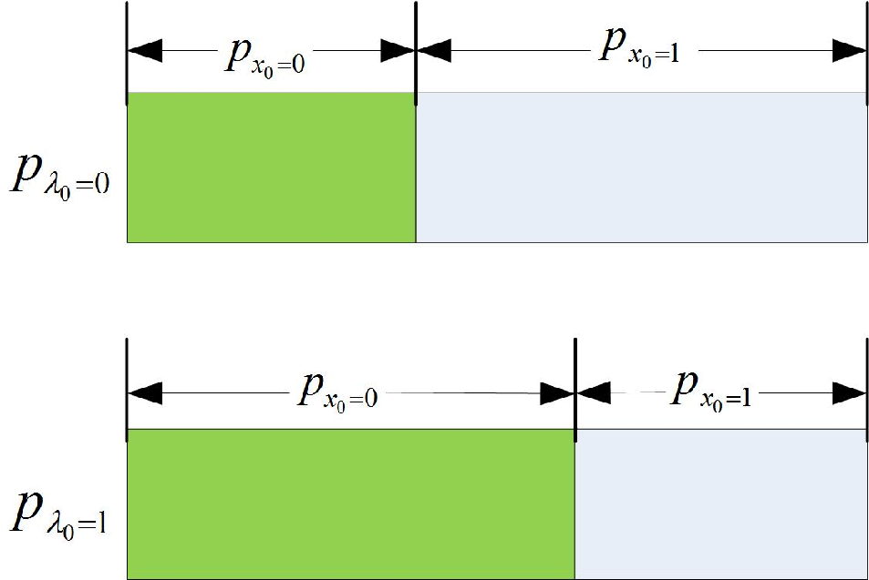
Similarly, we can also only observe the bases selection probability $p(x_{1})=p_{\lambda_{1}=0}p(x_{1}|\lambda_{1}=0)+p_{\lambda_{1}=1}p(x_{1}|\lambda_{1}=1)$, but the observed probability $p(x_{1})=\dfrac{1}{2}$ can’t guarantee $p(x_{1}|\lambda_{1}=0)=p(x_{1}|\lambda_{1}=1)=\dfrac{1}{2}$, the detailed bases selection deviation model is given in Fig. 4.

The practical quantum state preparation is given by

where

For given hidden variables $\lambda_{0}$ and $\lambda_{1}$, the difference between the phase error rate in the rectilinear basis and bit error rate in the diagonal basis can be given by

where $e_{p{\lambda_{0}}{\lambda_{1}}0}=\langle\phi_{3}|\rho_{AB_{Z\lambda_{0}}}|\phi_{3}\rangle+\langle\phi_{4}|\rho_{AB_{Z\lambda_{0}}}|\phi_{4}\rangle$, $e_{b{\lambda_{0}}{\lambda_{1}}1}=\langle\phi_{2}|\rho_{AB_{X\lambda_{0}}}|\phi_{2}\rangle+\langle\phi_{4}|\rho_{AB_{X\lambda_{0}}}|\phi_{4}\rangle$. Similarly, The difference between the phase error rate in the diagonal basis and bit error rate in the rectilinear basis can be given by

where $e_{p{\lambda_{0}}{\lambda_{1}}1}=\langle\phi_{3}|\rho_{AB_{X\lambda_{0}}}|\phi_{3}\rangle+\langle\phi_{4}|\rho_{AB_{X\lambda_{0}}}|\phi_{4}\rangle$, $e_{b{\lambda_{0}}{\lambda_{1}}0}=\langle\phi_{2}|\rho_{AB_{Z\lambda_{0}}}|\phi_{2}\rangle+\langle\phi_{4}|\rho_{AB_{Z\lambda_{0}}}|\phi_{4}\rangle$. By considering $e_{p{\lambda_{1}}0}=\langle\phi_{3}|\sum_{{\lambda_{0}}}p_{\lambda_{0}}\rho_{AB_{Z\lambda_{0}}}|\phi_{3}\rangle+\langle\phi_{4}|\sum_{{\lambda_{0}}}p_{\lambda_{0}}\rho_{AB_{Z\lambda_{0}}}|\phi_{4}\rangle=\sum_{\lambda_{0}}p_{\lambda_{0}}e_{p{\lambda_{0}}{\lambda_{1}}0}$ and $e_{b{\lambda_{1}}1}=\langle\phi_{2}|\sum_{{\lambda_{0}}}p_{\lambda_{0}}\rho_{AB_{X\lambda_{0}}}|\phi_{2}\rangle+\langle\phi_{4}|\sum_{{\lambda_{0}}}p_{\lambda_{0}}\rho_{AB_{X\lambda_{0}}}|\phi_{4}\rangle=\sum_{\lambda_{0}}p_{\lambda_{0}}e_{b{\lambda_{0}}{\lambda_{1}}1}$, we calculate the difference between the phase error rate $e_{p{\lambda_{1}}0}$ and the bit error rate $e_{b{\lambda_{1}}1}$

Similarly, the difference between $e_{p{\lambda_{1}}1}$ and $e_{b{\lambda_{1}}0}$ is

The probability of getting the rectilinear basis and diagonal basis measurement outcomes in Bob’s side can be respectively given by

where $p_{rec1}=p_{{\lambda_{1}}=0}p(x_{1}=0|{\lambda_{1}}=0),~p_{rec2}=p_{{\lambda_{1}}=1}p(x_{1}=0|{\lambda_{1}}=1),~~p_{dia1}=p_{{\lambda_{1}}=0}p(x_{1}=1|{\lambda_{1}}=0),~p_{dia2}=p_{{\lambda_{1}}=1}p(x_{1}=1|{\lambda_{1}}=1)$. The phase error rate in the rectilinear basis and diagonal basis can be respectively given by

The bit error rate in the rectilinear basis and diagonal basis can be respectively given by

By applying the two-step post processing method with the two different bases measurement outcomes, the final secret key rate can be given by

where the first part is the secret key generated by the rectilinear basis, while the second part is the secret key generated by the diagonal basis. The corresponding secret key rate $R$ with different quantum bit error rate values is given in Fig. 2, the calculation is based on the nonlinear optimization method with given quantum bit error rate, the detailed explanation is in the methods. To explain our analysis result, we compare the two analysis methods by considering the wavelength attack has the coupling ratio $0.4$ and $0.6$ with different wavelengths. If the observed quantum bit error rate is $0.02$, one-step post processing method can generate the secret key rate $0.0984$, while the two-step post processing method can generate the secret key rate $0.6642$.

Methods- By considering Eve’s arbitrary attacking scheme, the final secret key rate with two different bases can be calculated with the following optimization method

where $Q$ is the quantum bit error rate estimated in the practical experimental realization, $p_{rec}=p_{dia}=\dfrac{1}{2}$ are the bases selection probability observed in the practical experimental realization.

Conclusion - In this work, security of BB84 QKD protocol again the strong randomness attack and the weak randomness attack have been analyzed, which satisfies several practical attacking schemes, such as the photon number splitting attack, detector blinding attack, wavelength attack and time shift attack. We demonstrate that security of the practical QKD system can be evaluated by respectively considering the Trojan horse attack, the strong randomness attack and the weak randomness attack, and the three attacking models can be employed to build the practical QKD system security standardization in the future.

Acknowledgements - The authors are supported by the the National Natural Science Foundation of China (Grant Nos. 11304397, 61201239, 61205118 and 61475148), China Postdoctoral Science Foundation (Grant No. 2013M540514) and Anhui Provincial Natural Science Foundation(Grant No. 1408085QF102).

References

- [1] Bennett, C. H., Brassard, G., Quantum cryptography: Public-key distribution and coin tossing, Proceedings IEEE Int. Conf. on Computers, Systems and Signal Processing, Bangalore, India, pp. 175-179 (IEEE, New York, 1984).
- [2] Lo, H. K., Chau, H. F., Unconditional security of quantum key distribution over arbitrarily long distances. Science 283, 5410 (1999).
- [3] Shor, P., Preskill, J., Simple proof of security of the BB84 quantum key distribution protocol. Phys. Rev. Lett. 85, 441-444 (2000).
- [4] Renner, R., Security of Quantum Key Distribution. PhD thesis, Diss. ETH No 16242, quant-ph/0512258 (2005).
- [5] Kraus, B., Gisin, N., Renner, R., Lower and Upper Bounds on the Secret-Key Rate for Quantum Key Distribution Protocols Using One-Way Classical Communication. Phys. Rev. Lett. 95, 080501(2005).
- [6] Renner, R., Gisin, N., Kraus, B., Information-theoretic security proof for quantum-key-distribution protocols. Phys. Rev. A 72, 012332 (2005).
- [7] Scarani, V. et al. The security of practical quantum key distribution. Rev. Mod. Phys. 81, 1301-1350 (2009).
- [8] Gisin, N., Fasel, S., Kraus, B., Zbinden, H., and Ribordy, G., Trojan-horse attacks on quantum-key-distribution systems. Phys. Rev. A, 73, 022320 (2006).
- [9] Lutkenhaus, N., Estimates for practical quantum cryptography. Phys. Rev. A, 59, 3301 (1999).
- [10] Lutkenhaus, N., Security against individual attacks for realistic quantum key distribution. Phys. Rev. A, 61, 052304 (2000).
- [11] Lydersen, L., Wiechers, C., Wittmann, C., Elser, D., Skaar, J., and Makarov, V., Hacking commercial quantum cryptography systems by tailored bright illumination. Nature Photonics, 4, 686-689 (2010).
- [12] Yuan, Z. L., Dynes J. F., and Shields, A. J., Avoiding the blinding attack in QKD. Nature Photonics, 4, 800 (2010).
- [13] Qian, Y. J., Li, H. W., He, D. Y., Yin, Z. Q., Zhang, C. M., Chen, W., Wang, S., Han, Z. F., Countermeasure against probabilistic blinding attack in practical quantum key distribution systems, Chin. Phys. B, Vol. 24, No. 9, 090305 (2015).
- [14] Gottesman, D., Lo, H. K., Lutkenhaus, N., and Preskill, J., Security of quantum key distribution with imperfect devices. Quant. Inf. Comput., 5, 325-360 (2004).
- [15] Hwang, W. Y., Quantum Key Distribution with High Loss: Toward Global Secure Communication. Phys. Rev. Lett., 91, 057901 (2003).
- [16] Wang, X. B., Phys. Rev. Lett., Beating the photon-number-splitting attack in practical quantum cryptography. 94, 230503 (2005).
- [17] Lo, H. K., Ma, X., and Chen, K., Decoy State Quantum Key Distribution. Phys. Rev. Lett., 94, 230504 (2005).
- [18] Devetak, I., and Winter, A., Distillation of secret key and entanglement from quantum states. Proc. R. Soc. Lond. A 461 (2005).
- [19] Bouda, J., Pivoluska, M., Plesch, M. and Wilmott. C, Weak randomness seriously limits the security of quantum key distribution. Phys. Rev. A, 86, 062308 (2012).
- [20] Li, H. W., et al., Attacking a practical quantum-key-distribution system with wavelength-dependent beam-splitter and multiwavelength sources. Phys. Rev. A, 84, 062308 (2011).
- [21] Qi, B., Fung, C. H. F., Lo, H. K., and Ma, X., Time-shift attack in practical quantum cryptosystems. Quantum Inf. Comput., 7, 73-82 (2007).