OCReP: An Optimally Conditioned Regularization for Pseudoinversion
Based Neural Training
Abstract
In this paper we consider the training of single hidden layer neural networks by pseudoinversion, which, in spite of its popularity, is sometimes affected by numerical instability issues. Regularization is known to be effective in such cases, so that we introduce, in the framework of Tikhonov regularization, a matricial reformulation of the problem which allows us to use the condition number as a diagnostic tool for identification of instability. By imposing well-conditioning requirements on the relevant matrices, our theoretical analysis allows the identification of an optimal value for the regularization parameter from the standpoint of stability. We compare with the value derived by cross-validation for overfitting control and optimisation of the generalization performance. We test our method for both regression and classification tasks. The proposed method is quite effective in terms of predictivity, often with some improvement on performance with respect to the reference cases considered. This approach, due to analytical determination of the regularization parameter, dramatically reduces the computational load required by many other techniques.
Keywords:
Regularization parameter , Condition number , Pseudoinversion , Numerical instability1 Introduction
In past decades Single Layer Feedforward Neural Networks (SLFN) training was mainly accomplished by iterative algorithms involving the repetition of learning steps aimed at minimising the error functional over the space of network parameters. These techniques often gave rise to methods slow and computationally expensive.
Researchers therefore have always been motivated to explore alternative algorithms and recently some new techniques based on matrix inversion have been developed. In the literature, they were initially employed to train radial basis function neural networks (Poggio and Girosi, 1990a): the idea of using them also for different neural architectures was suggested for instance in (Cancelliere, 2001).
The work by Huang et al. (see for instance (Huang et al., 2006)) gave rise to a great interest in neural network community: they presented the technique of Extreme Learning Machine (ELM) for which SLFNs with randomly chosen input weights and hidden layer biases can learn sets of observations with a desired precision, provided that activation functions in the hidden layer are infinitely differentiable. Besides, because of the use of linear output neurons, output weights determination can be brought back to linear systems solution, obtained via Moore-Penrose generalised inverse (or pseudoinverse) of the hidden layer output matrix; so doing iterative training is no more required.
Such techniques appear anyway to require more hidden units with respect to conventional neural network training algorithms to achieve comparable accuracy, as discussed in Yu and Deng (Yu and Deng, 2012).
Many application-oriented studies in the last years have been devoted to the use of these single-pass techniques, easy to implement and computationally fast; some are described e.g. in (Nguyen et al., 2010; Kohno et al., 2010; Ajorloo et al., 2007). A yearly conference is currently being held on the subject, the International Conference on Extreme Learning Machines, and the method is currently dealt with in some journal special issue, e.g. Soft Computing (Wang et al., 2012) and the International Journal of Uncertainty, Fuzziness and Knowledge-Based Systems (Wang, 2013).
Because of the possible presence of singular and almost singular matrices, pseudoinversion is known to be a powerful but numerically unstable method: nonetheless in the neural network community it is often used without singularity checks and evaluated through approximated methods.
In this paper we improve on the theoretical framework using singular value analysis to detect the occurrence of instability. Building on Tikhonov regularization, which is known to be effective in this context (Golub et al., 1999), we present a technique, named Optimally Conditioned Regularization for Pseudoinversion (OCReP), that replaces unstable, ill-posed problems with well-posed ones.
Our approach is based on the formal definition of a new matricial formulation that allows the use of condition number as diagnostic tool. In this context an optimal value for the regularization parameter is analytically derived by imposing well-conditioning requirements on the relevant matrices.
The issue of regularization parameter choice has often been identified as crucial in literature, and dealt with in a number of historical contributions: a conservative guess might put its published estimates at several dozens. Some of the most relevant works are mentioned in section 2, where the related theoretical background is recalled.
Its determination, mainly aimed at overfitting control, has often been done either experimentally via cross-validation, requiring heavy computational training procedures, or analytically under specific conditions on the matrices involved, sometimes hardly applicable to real datasets, as discussed in section 2.
In section 3 we present the basic concepts concerning input and output weights setting, and we recall the main ideas on ill-posedness, regularization and condition number.
In section 4 our matricial framework is introduced, and constraints on condition number are imposed in order to derive the optimal value for the regularization parameter.
In section 5 our diagnosis and control tool is tested on some applications selected from the UCI database and validated by comparison with the framework regularized via cross-validation and with the unregularized one.
The same datasets are used in section 6 to test the technique effectiveness: our performance is compared with those obtained in other regularized frameworks, originated in both statistical and neural domains.
2 Recap on ordinary least-square and ridge regression estimators
As stated in the introduction, pseudoinversion based neural training brings back output weights determination to linear systems solution: in this section we recall some general ideas on this issue, that in next sections will be specialized to deal with SLFN training.
The estimate of through ordinary least-squares (OLS) technique is a classical tool for solving the problem
| (1) |
where and are column -vectors, is a column -vector and is an matrix; is random, with expectation value zero and variance .
In (Hoerl, 1962) and (Hoerl and Kennard, 1970) the role of ordinary ridge regression (ORR) estimator as an alternative to the OLS estimator in the presence of multicollinearity is deeply analized. In statistics, multicollinearity (also collinearity) is a phenomenon in which two or more predictor variables in a multiple regression model are highly correlated, meaning that one can be linearly predicted from the others with a non-trivial degree of accuracy. In this situation, the coefficient estimates of the multiple regression may change erratically in response to small changes in the model or the data.
It is known in literature that there exist estimates of with smaller mean square error (MSE) than the unbiased, or Gauss-Markov, estimate (Golub et al., 1979; Berger, 1976)
| (2) |
Allowing for some bias may result in a significant variance reduction: this is known as the bias-variance dilemma (see e.g. (Tibshirani, 1996; Geman et al., 1992), whose effects on output weights determination will be deepened in section 3.2.
Hereafter we focus on the one parameter family of ridge estimates given by
| (3) |
It can be shown that is also the solution to the problem of finding the minimum over of
| (4) |
which is known as the method of regularization in the approximation theory literature (Golub et al., 1979); basing on it we will develop the theoretical framework for our work in the next sections.
There has always been a substantial amount of interest in estimating a good value of from the data: in addition to those already cited in this section a non-exhaustive list of well known or more recent papers is e.g (Hoerl and Kennard, 1976; Lawless and Wang, 1976; McDonald and Galarneau, 1975; Nordberg, 1982; Saleh and Kibria, 1993; Kibria, 2003; Khalaf and Shukur, 2005; Mardikyan and Cetin, 2008).
A meaningful review of these formulations is provided in (Dorugade and Kashid, 2010). They first define the matrix such that ( contains the eigen values of the matrix ); then they set and , and show that a great amount of different methods require the OLS estimates of and
| (5) |
| (6) |
to define effective ridge parameter values. It is important to note that often specific conditions on data are needed to evaluate these estimators.
In particular this applies to the expressions of the ridge parameter proposed by (Kibria, 2003) and (Hoerl and Kennard, 1970), that share the characteristic of being functions of the ratio between and a function of ; they will be used for comparison with our proposed method in section 6.
The alternative technique of generalised cross-validation (GCV) proposed by (Golub et al., 1979) provides a good estimate of from the data as the minimizer of
| (7) |
where
| (8) |
This solution is particularly interesting, since it does not require an estimate of : because of this, it will be one term of comparison with our experimental results in section 6.
In the next section we will show how the problem of finding a good solution to (1) applies to the context of pseudoinversion based neural training, specializing the involved relevant matricies to deal with this issue.
3 Main ideas on regularization and condition number theory
3.1 Generalised inverse matrix for weights setting
We deal with a standard SLFN with input neurons, hidden neurons and output neurons, non-linear activation functions in the hidden layer and linear activation functions in the output layer.
Considering a dataset of distinct training samples , where and , the learning process for a SLFN aims at producing the matrix of desired outputs when the matrix of all input instances is presented as input.
As stated in the introduction, in the pseudoinverse approach the matrix of input weights and hidden layer biases is randomly chosen and no longer modified: we name it . After having fixed , the hidden layer output matrix is completely determined; we underline that since , it is not invertible.
The use of linear output neurons allows to determine the output weight matrix in terms of the OLS solution to the problem , in analogy with eq.(1). Therefore from eq.(2), we have
| (9) |
According to (Penrose and Todd, 1956; Bishop, 2006)
| (10) |
is the Moore-Penrose pseudoinverse (or generalized inverse) of matrix , and it minimises the cost functional
| (11) |
Singular value decomposition (SVD) is a computationally simple and accurate way to compute the pseudoinverse (see for instance (Golub and Van Loan, 1996)), as follows.
Every matrix can be expressed as
| (12) |
where and are orthogonal matrices and is a rectangular diagonal matrix (i.e. a matrix with if ); its elements , called singular values, are non-negative. A common convention is to list the singular values in descending order, i.e.
| (13) |
where p = min , so that is uniquely determined.
The SVD of is then used to obtain the pseudoinverse matrix :
| (14) |
where is again a rectangular diagonal matrix whose elements are obtained by taking the reciprocal of each corresponding element: (see also (Rao and Mitra, 1971)). From eq.(9) we than have:
| (15) |
Remark
An interesting case occurs when only elements in
eq.(13)
are non-zero, i.e. ; in this case the rank of matrix is and is defined as:
| (16) |
as shown for instance in (Golub and Van Loan, 1996).
This is also often done in practice, for computational reasons, for elements smaller than a predefined threshold, thus actually computing an approximated version of the pseudoinverse matrix .
This approach is for example used by default for pseudoinverse evaluation by means of the Matlab pinv function 11 1 http://www.mathworks.com/help/matlab/ref/pinv.html., because the tool is widely used by many scientists for example in ELM context, each time that it is applied blindly, i.e. without having decided at what threshold to zero the small , an approximation a priori uncontrolled is introduced in evaluation.
3.2 Stability and generalization properties of regularization algorithms
A key property for any learning algorithm is stability: the learned mapping has to suffer only small changes in presence of small perturbations (for instance the deletion of one example in the training set).
Another important property is generalization: the performance on the training examples (empirical error) must be a good indicator of the performance on future examples (expected error), that is, the difference between the two must be small. An algorithm that guarantees good generalization predicts well if its empirical error is small.
Many studies in literature dealt with the connection between stability and generalization: the notion of stability has been investigated by several authors, e.g. by Devroye and Wagner (Devroye and Wagner, 1979) and Kearns and Ron (Kearns and Ron, 1999).
Poggio et al. in (Mukherjee et al., 2003) introduced a statistical form of leave-one-out stability, named , building on a cross-validation leave-one-out stability endowed with conditions on stability of both expected and empirical errors; they demonstrated that this condition is necessary and sufficient for generalization and consistency of the class of empirical risk minimization (ERM) learning algorithms, and that it is also a sufficient condition for generalisation for not ERM algorithms (see also (Poggio et al., 2004)).
To turn an original instable, ill-posed problem into a well-posed one, regularization methods of the form (4) are often used (Badeva and Morozov, 1991) and among them, Tikhonov regularization is one of the most common (Tikhonov and Arsenin, 1977; Tikhonov, 1963). It minimises the error functional
| (17) |
obtained adding to the cost functional in eq.(11) a penalty term that depends on a suitably chosen Tikhonov matrix . This issue has been discussed in its applications to neural networks in (Poggio and Girosi, 1990b), and surveyed in (Girosi et al., 1995; Haykin, 1999).
Besides, Bousquet and Elisseeff (Bousquet and Elisseeff, 2002) proposed the notion of uniform stability to characterize the generalization properties of an algorithm. Their results state that Tikhonov regularization algorithms are uniformly stable and that uniform stability implies good generalization (Mukherjee et al., 2006).
Regularization thus introduces a penalty function that not only improves on stability, making the problem less sensitive to initial conditions, but it is also important to contain model complexity avoiding overfitting.
The idea of penalizing by a square function of weights is also well known in neural literature as weight decay: a wide amount of articles have been devoted to this argument, and more generally to the advantage of regularization for the control of overfitting. Among them we recall (Hastie et al., 2009; Tibshirani, 1996; Bishop, 2006; Girosi et al., 1995; Fu, 1998; Gallinari and Cibas, 1999).
A frequent choice is , to give preference to solutions with smaller norm (Bishop, 2006), so eq. (17) can be rewritten as
| (18) |
We define the regularized solution of (18): it belongs to the family of ridge estimates described by eq.(3) and can be expressed as
| (19) |
or, as shohw in ((Fuhry and Reichel, 2012)) as
| (20) |
and are from the singular value decomposition of (eq.(12)) and is a rectangular diagonal matrix whose elements, built using the singular values of matrix , are:
| (21) |
We remark on the difference between the minima of the regularized and unregularized error functionals. Increasing values of the regularization parameter induce larger and larger departure of the former (eq. (19)) from the latter (eq. (9)). Thus, the regularization process increases the bias of the approximating solution and reduces its variance, as discussed about the bias-variance dilemma in section 2.
3.3 Condition number as a measure of ill-posedness
The condition number of a matrix is the number defined as
| (22) |
where is any matrix norm. If the columns (rows) of are linearly independent, e.g. in case of experimental data matrices, then is a left (right) inverse of , i.e. . The Cauchy-Schwarz inequality in this case then provides ; besides, .
Matrices are said to be ill-conditioned if .
If norm is used, then
| (23) |
where and are the largest and smallest singular values of respectively.
From eq.(23) we can easily understand that large condition numbers suggest the presence of very small singular values (i.e. of almost singular matrices), whose numerical inversion, required to evaluate and the unregularized solution , is a cause of instability.
From numeric linear algebra we also know that if the condition number is large the problem of finding least-squares solutions to the corresponding system of linear equations is ill-posed, i.e. even a small perturbation in the data can lead to huge perturbations in the entries of solution (see (Golub and Van Loan, 1996)).
According to (Mukherjee et al., 2006) the stability of Tikhonov regularization algorithms can also be characterized using the classical notion of condition number: our proposed regularization method fits within this context. We will see that it specifically aims at analitically determining the value of the parameter that minimizes the conditioning of the regularized hidden layer output matrix so that the solution is stable in the sense of eq.(2.9) of (Mukherjee et al., 2006).
In the next section, we will derive the optimal value of the regularization parameter according to this stability criterion (minimum condition number).
The experimental results presented in sections 5 and 6 will evidence that our quest for stable solutions allows us to also achieve good generalization and predictivity. A comparison will be made to this purpose with the performance obtained when is determined via the standard cross-validation approach, aimed at overfitting control and generalization performance optimization.
4 Conditioning of the regularized matricial framework
For convenient implementation of our diagnostics, and building on eq.(20), we propose an original matricial framework in which to develop our study tool with the following definition.
Definition 1.
We define the matrix
| (24) |
as the regularized hidden layer output matrix of the neural network.
By construction, is decomposed in three matrices according to the SVD framework, and its singular values are provided by eq.(21) as a function of the singular values of .
This new regularized matricial framework makes easier the comparison of the properties of with those of the corresponding unregularized matrix . In fact, when unregularized pseudoinversion is used, nothing prevents the occurrence of very small singular values that make numerically instable the evaluation of (see eq. 14). On the contrary, even in presence of very small values of the original unregularized problem, a careful choice of the parameter allows to tune the singular values of the regularized matrix , preventing numerical instability.
4.1 Condition number definition
According to eq. (23), we define the condition number of as:
| (26) |
where and are the largest and smallest singular values of .
The shape of the functional relation that links regularized and unregularized singular values, defined through eq. (21), is shown in Fig.1 for three different values of .
The curves are non-negative, because and , and have only one maximum, with coordinates .
A few pairs of corresponding values are marked by dots on each curve.

For the sake of the determination of we are interested in evaluating and of over the finite, discrete range .
The value is reached in correspondence to a given singular value of , a priori not known, that we label , so that:
| (27) |
The variation of has the effect of changing the curve and shifting its maximum point within the interval . Therefore, can coincide with any singular value of from eq. (13), including the extreme ones.
Conversely, we now demonstrate that can only be reached in correspondence to or (or both when coincident).
Theorem 3.1
The minimum singular value of matrix can only be reached in correspondence to the largest singular value or to the smallest singular value of the unregularized matrix (or both).
Proof.
Without loss of generality, we can express as a function of , i.e. , where is a real positive value. By replacement in eq. (21), we get
To establish their ordering, we evaluate the difference of their inverses:
Recalling that , we can distinguish three cases:
- Case 1,
-
Because of the distribution shape, is also the minimum among all values , so that .
- Case 2,
-
Then, is also the minimum among all values , so that .
- Case 3,
-
Thus, and are both minima, so that .
∎
4.2 Condition number evaluation
The result by Theorem 3.1 allows us to find, according to eq. (26), the following expressions for :
Case 1, :
Case 2, :
Case 3, :
Bearing in mind that well-conditioned problems are characterized by small condition numbers, we now will look for the parameter values which, in the three cases above, make the regularized condition number smaller.

In Case 1, is an increasing function of , so that in its domain, i.e. , its minimum value is reached when . On the contrary, in Case 2, is a decreasing function of , so that in its domain, i.e. , the minimum is reached when .
Fig.2 shows the function behaviour over the whole domain.
Both cases have a common limit:
| (28) |
Such value is just that provided by Case 3, which can therefore be considered the best possible choice to minimize the condition number.
Thus our quest for the best possible conditioning for the matrix identifies an explicit optimal value for the regularization parameter :
| (29) |
5 Simulation and Discussion
For the numerical experimentation, we use eight benchmark datasets from the UCI repository (Bache and Lichman, 2013) listed in Table 1. All simulations are carried out in Matlab 7.3 environment.
The performance is assessed by statistics over a set of 50 different extractions of input weigths, computing either the average RMSE (for regression tasks) or the average percentage of misclassification rate (for classification tasks) on the test set. Either quantity is labeled “Err" in the tables summarising our results. The error standard deviation (labeled “Std") is also computed to evidence the dispersion of experimental results.
Our regularization strategy, labeled Optimally Conditioned Regularization for Pseudoinversion (OCReP), is verified by simulation against the common approach in which cross-validation is used i) to determine the regularization parameter at a fixed high number of hidden neurons and ii) to perform also hidden neurons number optimization, respectively in sec. 5.1 and 5.2.
A discussion of the effectiveness of OCReP in terms of minimization of the condition number of the involved matricies is done in sec. 5.3.
| Dataset | Type | N. Instances | N. Attributes | N. Classes |
|---|---|---|---|---|
| Abalone | Regression | 4177 | 8 | - |
| Machine Cpu | Regression | 209 | 6 | - |
| Delta Ailerons | Regression | 7129 | 5 | - |
| Housing | Regression | 506 | 13 | - |
| Iris | Classification | 150 | 4 | 3 |
| Diabetes | Classification | 768 | 8 | 2 |
| Wine | Classification | 178 | 13 | 3 |
| Segment | Classification | 2310 | 19 | 7 |
5.1 OCReP performance assessment: fixed number of hidden units
In this section we compare OCReP with a regularization approach in which is selected by a cross-validation scheme, which is typically used for control of under/overfitting and optimization of the model generalization performance. A 70%/30% split between training and test set is applied; then, a three-fold cross-validation search on the training set identifies the best by best performance on the validation set, over the set of 50 values of .
For the sake of comparison, a fixed, high number of hidden units is used, selected according to dimension and complexity of the datasets. For the three datasets Machine Cpu, Iris and Wine the simulation is performed for 50 and 100 hidden neurons; for Abalone, Delta Ailerons, Housing and Diabetes, we use 50, 100, 200 and 300 neurons; for Segment, we use 1000 and 1500 units.
Figures 3 and 4 (respectively for regression and classification datasets) show average test errors as a function of the sampled values of (red dots); the standard deviation is shown as an error bar. Our proposed optimal is evidenced as a blue circle, whereas the value of selected by cross-validation is shown as a black square. The results are in each case related to the highest number of neurons experimented.
The horizontal axis has been zoomed in onto the region of interest, i.e. .


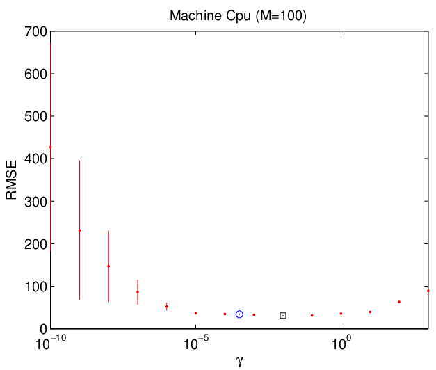

It may be noted that the performance from OCReP and cross-validation are comparable, and also close to the experimental minimum. This may be interpreted as good predictivity for both algorithms.
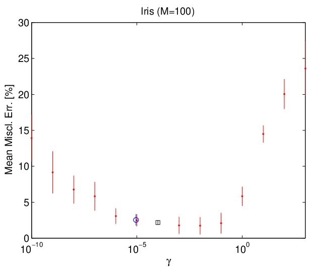


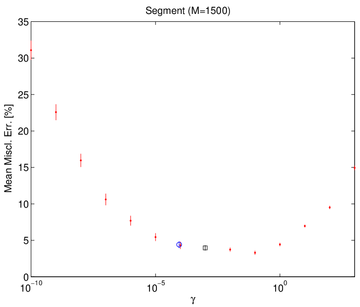
Also, we remark that the error bars, i.e. experimental result dispersion, is large for small values of , consistently with expectations on ineffective regularization.
| Iris | Wine | Machine Cpu | ||||
|---|---|---|---|---|---|---|
| OCReP | Err. | |||||
| Std | ||||||
| cross-val. | Err. | |||||
| Std | ||||||
| OCReP | Err. | |||||
| Std | ||||||
| cross-val. | Err. | |||||
| Std | ||||||
| Segment | ||||
|---|---|---|---|---|
| OCReP | Err. | |||
| Std | ||||
| cross-val. | Err. | |||
| Std | ||||
| OCReP | Err. | |||
| Std | ||||
| cross-val. | Err. | |||
| Std | ||||
| Abalone | Delta Ailerons | Housing | Diabetes | ||||
|---|---|---|---|---|---|---|---|
| OCReP | Err. | ||||||
| Std | |||||||
| cross-val. | Err. | ||||||
| Std | |||||||
| OCReP | Err. | ||||||
| Std | |||||||
| cross-val. | Err. | ||||||
| Std | |||||||
| OCReP | Err. | ||||||
| Std | |||||||
| cross-val. | Err. | ||||||
| Std | |||||||
| OCReP | Err. | ||||||
| Std | |||||||
| cross-val. | Err. | ||||||
| Std | |||||||
The numerical results have been reported in Tab. 2, 3 and 4 according to the grouping based on dimension and complexity of the datasets.
For each dataset and selected number of hidden neurons , the best test error is evidenced in bold, whenever the difference is statistically significant22 2 The Student’s t-test has been used for assessing the statistical significance through determination of the confidence intervals related to confidence level..
Thus, for example, on Iris the best performance is achieved using 50 neurons by OCReP, and with 100 neurons by cross-validation. In some cases, e.g. Wine (50 neurons), there is no clear winner from statistical considerations, i.e. the best results are comparable, within the errors.
From the above results it appears that cross-validation has better test error performance on a number of datasets slightly higher, at fixed number of hidden neurons. However, it is important to evidence that the use of OCReP allows to save the hundreds of pseudoinversion steps required by cross-validation, wich is a crucial issue for practical implementation.
5.2 OCReP performance assessment: variable number of hidden units
In order to pursue the double aim of performance and hidden units optimization, a first interesting step is to give a look to the variation as a function of hidden layer dimension of error trends of unregularized models (i.e. models whose output weights are evaluated according to eq.(10)).
A context widely used among researchers using such techniques (see e.g. Helmy and Rasheed (2009); Huang et al. (2006)) is to use input weights distributed according to a random uniform distribution in the interval , and sigmoidal activation functions for hidden neurons: hereafter we name this framework Sigm-unreg.


Figures 5 and 6 show, respectively for regression and classification datasets, the average test error values, (over 50 different input weights selections) for both OCReP (blue line) and Sigm-unreg (red line) as a function of the number of hidden nodes, which is gradually increased by unity steps. In all cases, after an initial decrease the Sigm-unreg test error increases significantly.
On the contrary, the OCReP test error curves keep decreasing, albeit at slower and slower rate, thus showing also a good capability of overfitting control of the method.
We aim now at comparing the results obtained when the trade-off value of is searched by cross-validation, with the two different frameworks discussed so far, i.e. OCReP and Sigm-unreg.
A 70%/30% split between training and test set is applied; we then perform a three-fold cross-validation for the selection of the number of hidden neurons at which the minimum error is recorded in all cases. Test errors are again evaluated as the average of 50 different random choices of input weights.
The numerical results of the simulation are presented in Tables 5 and 6, respectively for regression and classification tasks, with their standard deviations (Std) and .
Best test errors are evidenced in bold, whenever the difference between OCReP and cross-validation is statistically significant.
We see that our proposed regularization technique provides, for regression datasets, performance comparable with the cross-validation option but always a better performance (with statistical significance at level) with respect to the unregularized case.
For classification datatsets in three cases out of four OCReP provides a better performance with respect to cross-validation, and always a better performance with respect to the Sigm-unreg case. In all such cases, the statistical significance is at the level.
Also, in almost all cases smaller standard deviations are associated with the OCReP method, suggesting a lower sensitivity to initial input weights conditions.
5.3 Additional considerations
The proposed method OCReP presents in our opinion two features of interest: on one side, its computational efficiency, and on the other side its optimal conditioning.
Our goal of optimal analytic determination of the regularization parameter results in a dramatic improvement in the computing requirements with respect to experimental tuning by search over a pre-defined large grid of tentative values. In the latter case, for each choice of over the selected range, at least a pseudoinversion is required for every output weight determination, thus increasing the computational load by a factor .


Besides, our method is designed explicitly for optimal conditioning. In our simulations, we verify that the goal is fulfilled by evaluating average condition numbers of hidden layer output matrices. The statistics is performed over 50 different configurations of input weights and a fixed number of hidden units, namely the largest used in section 5.1 for each dataset. The results are summarised in Tables 7 and 8, respectively for regression and classification datasets. On the first row of each table, we list the ratio of average condition numbers of matrices , and , associated respectively to OCReP and Sigm-unreg, i.e. regularized and unregularized approaches. On the second row, we list the ratio of average condition numbers of matrices and , thus comparing our regularization approach with the more conventional one, the latter using cross-validation.
Not surprisingly, our regularization method provides a significant improvement on conditioning with respect to the unregularized approach, as evidenced by ratio values much smaller than unity. Besides, OCReP also provides better conditioned matrices than those derived by selection of through cross-validation, since the corresponding condition numbers are systematically smaller in the former case, sometimes up to an order of magnitude.
| Abalone | Housing | Delta Ailerons | Machine Cpu | |
| OCReP | ||||
| Err. | ||||
| Std. | ||||
| Cross-validation | ||||
| Err. | ||||
| Std. | ||||
| Sigm-unreg | ||||
| Err. | ||||
| Std. | ||||
| Iris | Wine | Diabetes | Segment | |
| OCReP | ||||
| Err. | ||||
| Std. | ||||
| Cross-validation | ||||
| Err. | ||||
| Std. | ||||
| Sigm-unreg | ||||
| Err. | ||||
| Std. | ||||
| Abalone | Housing | Delta Ailerons | Machine Cpu | |
|---|---|---|---|---|
| Iris | Wine | Diabetes | Segment | |
|---|---|---|---|---|
6 Comparison with other approaches
Since the literature provides a host of different recipes for either the choice of the regularization parameter, or the actual regularization algorithm, hereafter we focus on a couple of specific frameworks.
| Iris | Wine | Machine Cpu | |||
|---|---|---|---|---|---|
| Err. | |||||
| Std | |||||
| Err. | |||||
| Std | |||||
| Segment | ||||
|---|---|---|---|---|
| Err. | ||||
| Std | ||||
| Err. | ||||
| Std | ||||
| Abalone | Housing | Delta Ailerons | Diabetes | ||||
|---|---|---|---|---|---|---|---|
| Err. | |||||||
| Std | |||||||
| Err. | |||||||
| Std | |||||||
| Err. | |||||||
| Std | |||||||
| Err. | |||||||
| Std | |||||||
6.1 Other choices of regularization parameter
Among the approaches mentioned in section 2, we primary select the technique of generalised cross-validation (GCV) from (Golub et al., 1979), described by eqs. (7) and (8), for comparison with our method. The main motivation for our choice is its independence on the estimate of the error variance , which is a characteristic shared with our case. For each dataset, we select the same fixed numbers of hidden units as in section 5.1: then for each case eq. (7) is minimized over the set of 50 values of and for 50 different configurations of input weights.
We evaluate the mean and standard deviation of the corresponding regularized test error, reported in Tables 9, 10 and 11. We also remind that the tabulated error “Err" is either the average RMSE for regression tasks, or the average misclassification rate for classification tasks; “Std" is the corresponding standard deviation. The performance comparison is based on statistical significance at level.
Whenever GCV provides test error values statistically better than OCReP (listed in Tab. 2, 3 and 4), they are marked in bold.
We remark that in all cases listed in Tab. 2 and 3 OCReP provides statistically better results than GCV. The situation of medium size datasets evidences a somewhat mixed behaviour: with 50 hidden neurons, GCV wins; with 100 neurons, for three out of four datasets (i.e. Abalone, Housing and Diabetes) the performance is statistically comparable. In all other cases of Tab. 4 OCReP again provides better statistical results than GCV.
We make two other comparisons, using the ridge estimates described in eq.(13) and eq.(9) of (Dorugade and Kashid, 2010), and proposed respectively by (Kibria, 2003) and (Hoerl and Kennard, 1970):
| (30) |
| (31) |
Our experimentation is made only for regression datasets because the theoretical background of (Dorugade and Kashid, 2010), and of most of other works referred in section 2, directly applies to the case in which the quantity in eq.(1) is a one column matrix. In our formulation is the desired target and it is a one-column matrix only for regression tasks.
For each dataset we applied both methods described by eq. 30 and 31; we select the same fixed numbers of hidden units as in section 5.1 and perform 50 experiments with different configuration of input weights.
Each step of pseudoinversion is regularized for each method with the corresponding value. We evaluate the mean and standard deviation of the regularized test errors, reported respectively in Tables 12 and 13.
Whenever the methods provide test error values statistically better than OCReP (listed in Tab. 2 and 4), they are marked in bold.
We remark that the method by Kibria obtains a better performance in two cases over sixteen, while OCReP in 12 cases over sixteen. Besides, the method by Hoerl and Kennard obtains a better performance in three cases over sixteen, while OCReP in eight cases over sixteen. For both methods, better performance is achieved only for the case of neurons.
It may be noted that with respect to processing requirements OCReP has clear advantages, since it requires only a SVD step for each determination of , while the above two methods require full spectral decomposition and an additional matrix inversion.
6.2 Alternative regularization methods
A first comparison can be done with the work by Huang et al. (Huang et al., 2012), whose technique Extreme Learning Machine (ELM) uses a cost parameter that can be considered as related to the inverse of our regularization parameter . As authors state, in order to achieve good generalization performance, needs to be chosen appropriately. They do this by trying 50 different values of this parameter: .
A fair comparison can be done on our classification datasets, using their number of hidden neurons, i.e. 1000. Our optimal choice of allows to obtain a better performance on all datasets (with statistical significance assessed at the same confidence level that previous experiments).
| Abalone | Housing | Delta Ailerons | Machine Cpu | ||||
|---|---|---|---|---|---|---|---|
| Err. | |||||||
| Std | |||||||
| Err. | |||||||
| Std | |||||||
| Err. | |||||||
| Std | |||||||
| Err. | |||||||
| Std | |||||||
| Abalone | Housing | Delta Ailerons | Machine Cpu | ||||
|---|---|---|---|---|---|---|---|
| Err. | |||||||
| Std | |||||||
| Err. | |||||||
| Std | |||||||
| Err. | |||||||
| Std | |||||||
| Err. | |||||||
| Std | |||||||
| Iris | Wine | Diabetes | Segment | ||
|---|---|---|---|---|---|
| OCReP | Err. | ||||
| Std. | |||||
| ELM | Err. | ||||
| Std | |||||
Deng et al. (Deng et al., 2009) propose a Regularized Extreme Learning Machine (hereafter, RELM) in wich the regularization parameter is selected according to a similar criterion among 100 values: . Because their performance is optimized with respect to the number of hidden neurons, for the sake of comparison we use OCReP values from table 6. We obtain a statistically significant better performance on dataset Segment, while for Diabetes the method RELM performs better (see table 15).
| Diabetes | Segment | ||
|---|---|---|---|
| OCReP | Err. | ||
| Std. | |||
| RELM | Err. | ||
| Std. | |||
Comparing our results on the common regression datasets with the alternative method TROP-ELM proposed by Miche et al. (Miche et al., 2011), we note that OCReP achieves always lower RMSE values 33 3 In that work, performance and related statistics are expressed in terms of MSE; we only derived the corresponding RMSE for comparison with our results. (with statistical significance), as can be seen from table 16.
Besides, in our opinion our method is simpler, in the sense that it uses a single step of regularization rather than two.
| Abalone | Delta Ailerons | Machine Cpu | Housing | ||
| OCReP | Err. | ||||
| Std. | |||||
| TROP-ELM | Err. | ||||
In (Martinez-Martinez et al., 2011), an algorithm is proposed for pruning ELM networks by using regularized regression methods: the crucial step of regularization parameter determination is solved by creating different models, each one based on a different value of this parameter, among which the best one is selected using a Bayesian information criterion. Authors state that a typical value for is 100, thus an heavy computational load is required, and the method is focused on regression tasks.
7 Conclusions
In the context of regularization techniques for single hidden layer neural networks trained by pseudoinversion, we provide an optimal value of the regularization parameter by analytic derivation. This is achieved by defining a convenient regularized matricial formulation in the framework of Singular Value Decomposition, in which the regularization parameter is derived under the constraint of condition number minimization. The OCReP method has been tested on UCI datasets for both regression and classification tasks. For all cases, regularization implemented using the analytically derived is proven to be very effective in terms of predictivity, as evidenced by comparison with implementations of other approaches from the literature, including cross-validation. OCReP avoids hundreds of pseudoinversions usually needed by most other methods, i.e. it is quite computationally attractive.
Acknowledgements
The activity has been partially carried on in the context of the Visiting Professor Program of the Gruppo Nazionale per il Calcolo Scientifico (GNCS) of the Italian Istituto Nazionale di Alta Matematica (INdAM). This work has been partially supported by ASI contracts (Gaia Mission - The Italian Participation to DPAC) I/058/10/0-1 and 2014-025-R.0.
References
- Ajorloo et al. (2007) Ajorloo, H., Manzuri-Shalmani, M. T., and Lakdashti, A. (2007). Restoration of damaged slices in images using matrix pseudo inversion. In Proceedings of the 22nd International symposium on computer and information sciences, pages 1–6.
- Bache and Lichman (2013) Bache, K. and Lichman, M. (2013). UCI machine learning repository.
- Badeva and Morozov (1991) Badeva, V. and Morozov, V. (1991). Problèmes incorrectement posés: Théorie et applications en identification , filtrage optimal, contrôle optimal, analyse et synthèse de systèmes, reconnaissance d’images. Série Automatique. Masson.
- Berger (1976) Berger, J. (1976). Minimax estimation of a multivariate normal mean under arbitrary quadratic loss. J. Multivariate Analysis, 6, 256–264.
- Bishop (2006) Bishop, C. M. (2006). Pattern Recognition and Machine Learning (Information Science and Statistics). Springer-Verlag New York, Inc., Secaucus, NJ, USA.
- Bousquet and Elisseeff (2002) Bousquet, O. and Elisseeff, A. (2002). Stability and generalization. J. Mach. Learn. Res., 2, 499–526.
- Cancelliere (2001) Cancelliere, R. (2001). A high parallel procedure to initialize the output weights of a radial basis function or bp neural network. In Proceedings of the 5th International Workshop on Applied Parallel Computing, New Paradigms for HPC in Industry and Academia, PARA ’00, pages 384–390, London, UK, UK. Springer-Verlag.
- Deng et al. (2009) Deng, W., Zheng, Q., and Chen, L. (2009). Regularised extreme learning machine. In Proceedings of the IEEE Symposium on Computational Intelligence and Data Mining.
- Devroye and Wagner (1979) Devroye, L. P. and Wagner, T. (1979). Distribution-free performance bounds for potential function rules. Information Theory, IEEE Transactions on, 25(5), 601–604.
- Dorugade and Kashid (2010) Dorugade, A. and Kashid, D. (2010). Alternative method for choosing ridge parameter for regression. Applied Mathematical Sciences, 4, 447–456.
- Fu (1998) Fu, W. (1998). Penalized regressions: the bridge vs. the lasso. Journal of Computational and Graphical Statistics, 7, 397–416.
- Fuhry and Reichel (2012) Fuhry, M. and Reichel, L. (2012). A new tikhonov regularization method. Numerical Algorithms, 59(3), 433–445.
- Gallinari and Cibas (1999) Gallinari, P. and Cibas, T. (1999). Practical complexity control in multilayer perceptrons. Signal Processing, 74, 29–46.
- Geman et al. (1992) Geman, S., Bienenstock, E., and Doursat, R. (1992). Neural networks and the bias/variance dilemma. Neural Computation, 4, 1–58.
- Girosi et al. (1995) Girosi, F., Jones, M., and Poggio, T. (1995). Regularization Theory and Neural Networks Architectures. Neural Computation, 7, 219–269.
- Golub et al. (1979) Golub, G., heath, M., and Wahba, G. (1979). Generalized cross-validation as a method for choosing a good ridge parameter. Technometrics, 21, 215–223.
- Golub and Van Loan (1996) Golub, G. H. and Van Loan, C. F. (1996). Matrix computations (3rd ed.). Johns Hopkins University Press, Baltimore, MD, USA.
- Golub et al. (1999) Golub, G. H., Hansen, P. C., and O’Leary, D. P. (1999). Tikhonov regularization and total least squares. SIAM J. Matrix Anal. Appl., 21(1), 185–194.
- Hastie et al. (2009) Hastie, T., Tibshirani, R., and Friedman, J. (2009). The elements of Statistical Learning: Data Mining, Inference, and Prediction (2rd ed.). Springer.
- Haykin (1999) Haykin, S. (1999). Neural Networks: A Comprehensive Foundation. International edition. Prentice Hall.
- Helmy and Rasheed (2009) Helmy, T. and Rasheed, Z. (2009). Multi-category bioinformatics dataset classification using extreme learning machine. In Proceedings of the Eleventh conference on Congress on Evolutionary Computation, CEC’09, pages 3234–3240, Piscataway, NJ, USA. IEEE Press.
- Hoerl (1962) Hoerl, A. (1962). Application of ridge analysis to regression problems. Chemical Engineering Progress, 58, 54–59.
- Hoerl and Kennard (1970) Hoerl, A. and Kennard, R. (1970). Ridge regression: Biased estimation for nonorthogonal problems. Technometrics, 12, 55–67.
- Hoerl and Kennard (1976) Hoerl, A. and Kennard, R. (1976). Ridge regression: iterative estimation of the biasing parameter. Communications in Statistics, A5, 77–88.
- Huang et al. (2006) Huang, G.-B., Zhu, Q.-Y., and Siew, C.-K. (2006). Extreme learning machine: theory and applications. Neurocomputing, 70(1), 489–501.
- Huang et al. (2012) Huang, G.-B., Zhu, Q.-Y., and Siew, C.-K. (2012). Extreme learning machine for regression and multiclass classification. IEEE Transactions on Systems, Man, and Cybernetics–Part B: Cybernetics, 42(2), 513–529.
- Kearns and Ron (1999) Kearns, M. and Ron, D. (1999). Algorithmic stability and sanity-check bounds for leave-one-out cross-validation. Neural Computation, 11(6), 1427–1453.
- Khalaf and Shukur (2005) Khalaf, G. and Shukur, G. (2005). Choosing ridge parameter for regression problem. Communications in Statistics – Theory and methods, 34, 1177–1182.
- Kibria (2003) Kibria, B. (2003). Performance of some new ridge regression estimators. Communications in Statistics – Simulation and Computation, 32, 419–435.
- Kohno et al. (2010) Kohno, K., Kawamoto, M., and Inouye, Y. (2010). A matrix pseudoinversion lemma and its application to block-based adaptive blind deconvolution for mimo systems. Trans. Cir. Sys. Part I, 57(7), 1449–1462.
- Lawless and Wang (1976) Lawless, J. and Wang, P. (1976). A simulation study of ridge and other regression estimators. Communications in Statistics, A5, 307–324.
- Mardikyan and Cetin (2008) Mardikyan, S. and Cetin, E. (2008). Efficient choice of biasing constant for ridge regression. International Journal of Contemporary Mathematical Sciences, 3, 527–547.
- Martinez-Martinez et al. (2011) Martinez-Martinez, J., Escandell-Montero, P., Soria-Olivas, E., Martı´n-Guerrero, J., Magdalena-Benedito, R., and Juan, G.-S. (2011). Regularized extreme learning machine for regression problems. Neurocomputing, 74, 3716–3721.
- McDonald and Galarneau (1975) McDonald, G. and Galarneau, D. (1975). A monte carlo evaluation of some ridge-type estimators. J. Amer. Statist. Assoc., 70, 407–416.
- Miche et al. (2011) Miche, Y., van Heeswijk, M., Bas, P., Simula, O., and Lendasse, A. (2011). Trop-elm: A double-regularized elm using lars and tikhonov regularization. Neurocomputing, 74(16), 2413 – 2421.
- Mukherjee et al. (2003) Mukherjee, S., Niyogi, P., Poggio, T., and Rifkin, R. (2003). Statistical learning: stability is sufficient for generalization and necessary and sufficient for consistency of empirical risk minimization. CBCL, Paper 223, Massachusetts Institute of Technology.
- Mukherjee et al. (2006) Mukherjee, S., Niyogi, P., Poggio, T., and Rifkin, R. (2006). Learning theory: stability is sufficient for generalization and necessary and sufficient for consistency of empirical risk minimization. Advances in Computational Mathematics, 25(1-3), 161–193.
- Nguyen et al. (2010) Nguyen, T. D., Pham, H. T. B., and Dang, V. H. (2010). An efficient pseudo inverse matrix-based solution for secure auditing. In Proceedings of the IEEE International Conference on Computing and Communication Technologies, Research, Innovation, and Vision for the Future, IEEE International Conference.
- Nordberg (1982) Nordberg, L. (1982). A procedure for determination of a good ridge parameter in linear regression. Communications in Statistics, A11, 285–309.
- Penrose and Todd (1956) Penrose, R. and Todd, J. A. (1956). On best approximate solutions of linear matrix equations. Mathematical Proceedings of the Cambridge Philosophical Society, null, 17–19.
- Poggio and Girosi (1990a) Poggio, T. and Girosi, F. (1990a). Networks for approximation and learning. Proceedings of the IEEE, 78(9), 1481–1497.
- Poggio and Girosi (1990b) Poggio, T. and Girosi, F. (1990b). Regularization algorithms for learning that are equivalent to multilayer networks. Science, 247(4945), 978–982.
- Poggio et al. (2004) Poggio, T., Rifkin, R., Mukherjee, S., and Niyogi, P. (2004). General conditions for predictivity in learning theory. Letters to Nature, 428, 419/422.
- Rao and Mitra (1971) Rao, C. and Mitra, S. (1971). Generalized inverse of matrices and its applications. Wiley series in probability and mathematical statistics: Applied probability and statistics. Wiley.
- Saleh and Kibria (1993) Saleh, A. and Kibria, B. (1993). Performances of some new preliminary test ridge regression estimators and their properties. Communications in Statistics – Theory and methods, 22, 2747–2764.
- Tibshirani (1996) Tibshirani, R. (1996). Regression shrinkage and selection via the lasso. Journal of Royal Statistical Society, 58, 267–288.
- Tikhonov and Arsenin (1977) Tikhonov, A. and Arsenin, V. (1977). Solutions of ill-posed problems. Scripta series in mathematics. Winston, Washington DC.
- Tikhonov (1963) Tikhonov, A. N. (1963). Solution of incorrectly formulated problems and the regularization method. Soviet Math. Dokl., 4, 1035–1038.
- Wang (2013) Wang, X. (2013). Special issue on extreme learning machines with uncertainty. Int. J. Unc. Fuzz. Knowl. Based Syst., 21.
- Wang et al. (2012) Wang, X.-Z., D., W., and Huang, G.-B. (2012). Special issue on extreme learning machines. Soft Computing, 16(9), 1461–1463.
- Yu and Deng (2012) Yu, D. and Deng, L. (2012). Efficient and effective algorithms for training single-hidden-layer neural networks. Pattern Recogn. Lett., 33(5), 554–558.