Wavelet subspace decomposition of thermal infrared images for defect detection in artworks
Abstract
Monitoring the health of ancient artworks requires adequate prudence because of the sensitive nature of these materials. Classical techniques for identifying the development of faults rely on acoustic testing. These techniques, being invasive, may result in causing permanent damage to the material, especially if the material is inspected periodically. Non destructive testing has been carried out for different materials since long. In this regard, non-invasive systems were developed based on infrared thermometry principle to identify the faults in artworks. The test artwork is heated and the thermal response of the different layers is captured with the help of a thermal infrared camera. However, prolonged heating risks overheating and thus causing damage to artworks and an alternate approach is to use pseudo-random binary sequence excitations. The faults in the artwork, though, cannot be detected on the captured images, especially if their strength is weak. The weaker faults are either masked by the stronger ones, by the pictorial layer of the artwork or by the non-uniform heating. This work addresses the detection and localization of the faults through a wavelet based subspace decomposition scheme. The proposed scheme, on one hand, allows to remove the background while, on the other hand, removes the undesired high frequency noise. It is shown that the detection parameter is proportional to the diameter and the depth of the fault. A criterion is proposed to select the optimal wavelet basis along with suitable level selection for wavelet decomposition and reconstruction. The proposed approach is tested on a laboratory developed test sample with known fault locations and dimensions as well as real artworks. A comparison with a previously reported method demonstrates the efficacy of the proposed approach for fault detection in artworks.
Index Terms:
Non-destructive testing, subspace decomposition, wavelet transform, fault detection, mutual information, Infrared thermography, PRBS excitationI Introduction
The detection and identification of faults in different materials has seen major emphasis over the last decades, both in research context and in industrial applications. Diverse techniques like Gamma and X-rays, ultrasounds, Foucault currents and Nuclear magnetic resonance are conventionally utilized for non-destructive testing of materials [1], [2], [3], [4], [5], [6], [7]. Recently, techniques focusing on thermal radiations, such as photo-reflectance, photo-acoustics, mirage effect and photo thermal radiometry, have been tested on the laboratory scale for non-invasive testing of materials [8]. One such technique is the photo-thermal radiometry (or photo-thermometry) which requires a relatively simple and low-cost experimental setup [9]. The test material is excited by a flow of heat, resulting in a change in local thermal conditions of the material. The thermal response of the material to this excitation is then captured by a thermal infrared camera. The acquired thermal response depends on different parameters of the material such as thermal conductivity, diffusivity, emissivity and specific heat as well as the excitation used at the input. More specifically, the above properties manifest themselves in the thermal response depending upon different factors such as fissures or holes in the material, material structure, physicochemical processes taking place in the material, delamination, sedimentation, etc. The detection of faults in ancient artworks is a challenging problem requiring adequate precaution to identify the faults without deteriorating the material, even slightly. The conventional method used for exciting the material is the pulse excitation method which consists of heating the material over a relatively long time and then allowing it to cool down [10]. In the current research endeavor the frescos(Italian murals) are the subject of interest which are layered structures. Due to the environmental effects air gaps occur at the interface of the layers. This is the working definition of a defect in the artwork which will be used through out the current paper. The acquired thermal response is relatively easier to process from fault identification purposes. However, the prolonged heating involved in the process risks overheating and thus causing damage to the material. An alternate approach is to use random excitations like the Gaussian and pseudo-random binary sequence (PRBS) excitations. The step heating results in a greater transfer of thermal energy to the material under analysis as compared to the PRBS excitation.In photo-thermal radiometry the detection of fault is based on the variations in the thermal radiations based on the presence of faults hence a greater transfer of thermal energy will yield better contrast. While these techniques are more favorable from material health conservation perspective, they necessitate more intensive processing to retrieve useful information about the defects.
The useful information should reveal the localization maps of different defects in the material after having suppressed the effects of pictorial layer, measurement noise, potential interference patterns due to multiple excitation sources and inhomogeneous illumination of the test material. Recently, some signal processing based methods were deployed for detecting defects in artworks while using PRBS excitations [11]. Although, the method revealed some interesting results regarding the material defects, the interpretation of the final results was not very evident. In this paper, we propose a new processing algorithm based on wavelet decomposition for identification of defects. The algorithm exploits the multi-resolution capability of wavelet transform and approximates an efficient subspace, which contains information on the defects, while removing other influences from the acquired thermal response. The proposed subspace decomposition approach is applied spatially and the resulting subspaces for different acquisitions are then temporally processed to extract a single representative subspace for the defects. Since there is no universal criterion for the selection of wavelet basis function, we propose a selection criterion as well as an automated mechanism for determining the wavelet decomposition level. Even though the main focus of the paper is proposition of a defect detection algorithm, it is demonstrated that the intensity of the final detection parameter can be associated to the intensity of the defect. The proposed method is validated on a sample test material, containing defects of various depths and diameters. The detection parameter allows localizing these faults in the test sample with different intensities. The method is also applied on a real artwork to reveal interesting information about the defects. The paper is organized to start with a presentation of the experimental setup, the test samples and the acquired data set. This is followed by the proposed methodology section comprising the mathematical formulation of the problem, the details of the proposed algorithm and the different parameters involved therein. The results of the proposed approach on a test sample are discussed in the subsequent section. The paper is finally concluded to highlight the pros and cons of the proposed approach along with an insight into some future work in the domain.
II Experimental Setup and Raw Data Set
In this section, the experimental setup for photo-radiometry system including the excitation and acquisition process is described, along with the presentation of a sample data set.


II-A Excitation and Acquisition System
The experimental setup for photo thermometry is illustrated in Figure 1(a). The artwork is heated simultaneously by two halogen lamps, each one with a power of W. The lamps are symmetrically placed around the infrared camera and placed at approximately cm from the artwork. The temporal excitation pattern of these two lamps is controlled by a pseudo random binary sequence (PRBS). The smallest duration of each binary pulse in this sequence represents the excitation time (). The experiment described in this paper is carried out for different excitation times as represented in Table I.This was done to demonstrate the generality of the proposed algorithm across different experimental parameters. An illustrative excitation pattern is shown in Figure 1(b).
The incident flow of heat strikes the surface of the material and its subsequent absorption depends on the physical properties of the material. The surface defects, such as cracks, might appear instantly due to the different optical properties and require other methods for detection. The sub-surface defects appear after some time depending on their respective depths. The major challenge is posed by the defects that are not visible at the surface and are located at different or varying depths. Such defects cause air pockets in otherwise uniform material, resulting in different distributions of the heat inside the materials. The radiated thermal energy is modified and presents an opportunity to identify the faults and to quantify them. In brief, different defects into a material exhibit different thermal responses to the same excitation.
The thermal response of these different areas subjected to the excitation sequence are then captured by a A FLIR thermal Infrared (IR) camera. This bolometer camera, working in long wavelength range ( to ) and having a thermal sensitivity of at , was placed around cm from the sample. The excitation of the lamp and the IR camera were synchronized, the former being in a slave mode. A thermal image is obtained for each pulse duration of the input PRBS sequence, the total number of such images is thus same as the number of pulses in the PRBS sequence, . The number of pulses in the PRBS sequences corresponding to the different excitation times is mentioned in Table I.
Even though, the relative positions of the halogen lamps and the camera have been carefully setup after exhaustive testing, the problem of inhomogeneous illumination can not be ruled out. It will be demonstrated that the proposed wavelet based subspace decomposition approach allows estimation of a background affect which may be attributed to inhomogeneous illumination. The preceding description of the experimental setup indicates that the thermal behavior of the material is spatially non-stationary. The subsequent sections will reveal how the proposed approach allows exploiting this spatial non-stationarity.
II-B Test Materials
Before developing a mathematical formulation for the problem of defect detection, we briefly shift our focus to the presentation of the test samples used in this work. In particular, we consider two types of test materials, one with faults of different dimensions simulated by introducing holes in a plaster material and other are real artworks containing faults of varying geometry and dimensions.
II-B1 Laboratory test sample
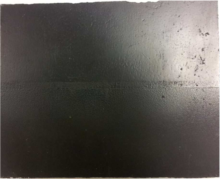
The complete acquisition chain of the experimental setup will be demonstrated with the help of this test material to enhance understanding of the underlying problem, which needs to be modeled. It will also serve as a ground truth against which different parameters of the proposed algorithm will be established. The test material is composed of a white plaster substrate with a thickness of approximately mm (Fig. 2). The front side of the material, which is exposed to the excitation, does not contain any significant defects, but still has some minor irregularities, especially toward the edges (Fig. 2(a)). As described earlier a defect in an artwork is typically characterized by the slight delamination of the material in the vicinity of the defect causing air pockets within the material. The back side of the material was therefore modified to create defects of different dimensions (Fig. 2(b)). In particular, differentiation amongst these defects arise from differences in their depths and diameters. Twelve different holes were created in the material and their dimensions (depths and diameters) are marked in Fig. 2(b) and also summarized in Table II. It is pertinent to mention that these depths are measured from the front side of the material. Thus, hole (Fig. 2(b) top right) is at a depth of mm from the front surface. The holes have been numbered in sequence starting from top right (hole ) and moving left and down to bottom left (hole ). As illustrated in Fig. 2(b), three different depths, ( mm, mm, and mm) with four different diameters ( mm, mm, mm, and mm) for each of these depths, have been tested in this experiment. It is assumed that each fault has uniform depth and diameter signifying that at the spatial location of the fault, there’s an air pocket across the material up till the depth of the given fault. As the surface is heated the thermal energy gradually diffuses through the depth of the material. The rate of the diffusion depends on the thermal diffusivity of the material. The thermal diffusivity of the plaster of Paris (the main constituent of the fresco) is greater than that of the air (present at the fault locations). This results in a difference in the rate of diffusion of heat and in result the amount of back scattered radiation results in detection of fault regions(as they present higher thermal intensity).

Shallower and wider faults offer bigger air pockets which effect the thermal diffusivity and conductivity. This translates physically into the mm hole (depth) more likely to depict a higher heat intensity as compared to the mm and mm holes. The overall impact on the outcome is that the acquired thermal response is more intense at the location of shallower and wider holes as compared to deeper and narrower holes.
| Hole | Coordinates(pixels) | Diameter | Depth | Improvement in SNR via proposed algorithm | |||||
| (mm) | (mm) | (dB) | |||||||
Photo-radiometry is an inspection technique, which works at depths closer to the contact surface [9]. While, the higher intensity faults may be identifiable in the raw thermal images, the smaller faults are often masked. The goal of this work is to extract such faults from the background. The test sample described above will also allow studying the influence of the diameter (spread) of a certain defect for a given depth. Moreover, it will reveal the impact of processing raw data through the proposed algorithm in terms of enhancing the detectability of the faults at different depths. It should be mentioned that real defects in an artwork will not necessarily be circular in shape, but the purpose of the current research is not to indulge in particular defect geometries but rather to establish the detectability limits. Nevertheless, the viability of the proposed approach for irregular defects will be demonstrated on real artworks in the results section.
II-B2 Real Artwork
In order to validate the proposed approach, thermal responses of a real artwork, namely Mural , were acquired. This artwork represents a replica of the “Saint Christopher with the Christ Child”, a Florentine fresco realized in the end of the century, created in laboratory according to the technique of the Italian primitives [11]. Fig. 3(a) shows a picture of Mural , along with the designated faults in this artwork (Fig. 3(b)). Five inclusions of plastazote have been introduced in the fresco in its manufacturing process. These five faults are labeled A to E: A is tilted with varying depths of to mm and a thickness of mm; B is at a depth of mm with a thickness varying between mm and mm; D is located at a depth of mm and has a thickness of mm; E is at a depth of mm, lying beneath D, and has a thickness of mm; finally, C is a powdery defect located at a depth of mm and has thickness of mm. These faults are of non-uniform shapes.
Another real artwork used during the course of this work is named Mural . No information regarding the position of the sub-surface faults is known prior to the application of the proposed algorithm. The surface artifact is a piece of gold foil which in the course of present investigation is not of interest and will hence be removed using post processing techniques as discussed later on.


III Proposed methodology: selective sub-space extraction for defect detection
In this section, we will present the proposed approach for the detection of defects. Before delving into the details of the algorithm, we will associate a mathematical formulation to the acquired thermal responses. Moreover, we will also briefly discuss a method previously developed by the authors in order to substantiate the merits of the approach proposed in this paper. The acquired raw data consist of thermal images, as shown in Fig. 4. Note that images acquired on the front side were flipped on the axis in order to have the same positioning of the holes shown in the back side (see Fig. 2(b)). The raw data cube, , exist in the Hilbert space , where and correspond to the dimension of the test material (pixels) as captured by the camera and corresponds to the total number of acquisitions in time (samples). While and will be fixed for a given test sample (assuming the experimental setup is not changed and the resolution of the camera is not exceeded), the value of will depend on the excitation time () as represented in the Table I. The raw data contains information from multiple sources including defects, background or pictorial layer, inhomogeneous illumination and measurement noise. The Hilbert space containing the raw data can be decomposed into its subspaces, each representing single or multiple afore mentioned sources. Subspace decomposition is a processing technique which allows more meaningful projections. In our case, we are looking to decompose the data into background, defect (useful) and noise subspaces. Subspace decomposition based matrix filtering techniques have been used in diverse applications [12], [13], [14], [15], [16]. Singular Value Decomposition (SVD) and Wavelet decomposition are common methods of sub-space decomposition. In this paper, the SVD based technique for defect identification will be compared with the proposed wavelet based decomposition technique.

III-A State-of-the-art decomposition of thermal responses
An SVD based defect detection scheme in artworks using the thermal responses was developed by Vrabie et al. [11]. The scheme was based on the hypothesis that the evolution of thermal response over time is a distinguishing factor between defects and background. It involved rearranging the data cube, into a -D data set , where , represents the spatial dimension. This -D space was then decomposed into three subspaces, the first one representing background, the second one useful information containing defects and the third one the noise components. The number of singular values to be considered for each of the three subspaces was determined empirically. Specifically, only one singular value containing of energy was used for extracting the background, whereas the so called useful subspace containing defects was synthesized from few subsequent components and the lowest energy singular components were attributed to the noise. The second subspace was selected for further processing to detect the locations of defects. The higher order statistics (HOS) of skewness and kurtosis were then computed for the time series in the useful subspace to obtain the results in space, which were then rearranged to obtain an image map in for both kurtosis and skewness. It was demonstrated that these skewness and kurtosis maps can help in identification of defects. However, the interpretation of the results obtained with this SVD and HOS based approach was not systematic.
Although, SVD is a matrix filtering technique, it was utilized in the temporal domain without any focus on explicitly exploiting the spatial patterns of the defects. The high energy first component of SVD contains information on the average behavior of the input data. Since, the SVD-HOS approach, discussed above, discards the first subspace, it therefore runs the risks of suppressing high energy defects along with the background. This fact is attributable to the poor separability of different components by a second-order statistics based approach such as SVD. The limitations of this SVD-HOS based approach led us to the development of an alternate approach for detection of defects. This multi-resolution analysis based approach also performs the subspace decomposition but in spatial rather than the temporal domain.
III-B Wavelet based subspace decomposition
The raw thermal response acquired by the camera at a given instant, , incorporates information on the defects but this information is often masked by many undesirable effects such as inhomogeneous illumination, background pictorial layer and measurement noise. The inhomogeneous illumination is caused by irradiation from two different sources whose placement, though carefully adjusted, could not make the captured image illumination invariant. The characteristics of the pictorial layer of the test material such as pattern and/or the paint also manifest themselves strongly in the acquired raw image. In addition, the defects can have different dimensions in terms of the wear-ability of the material. The stronger defects will have more significant intensities and will appear sooner as compared to the weaker ones because of the fact that for stronger defects (e.g. those closer to the surface), the heat diffusion will be greater as compared to weaker ones. The spatial pattern of the raw thermal image is therefore non-stationary. In order to better exploit this non-stationarity, we resort to the joint-time frequency analysis of wavelet transform. The underlying principle is that of the multi-resolution analysis whereby it is possible to decompose the input data into multiple subbands.
Discrete Wavelet Transform (DWT) is a powerful tool for performing multi-resolution analysis and has been exploited in numerous fault detection applications [15], [17], [18], [19], [20], [13]. At any level of decomposition ‘’, DWT decomposes the input data into a high pass or detail subspace and a low pass or approximation subspace , with input to the level being and to any subsequent level , the approximation of the previous level . To apply the DWT on -D datasets, the filtering is first applied along one dimension and then the resulting images are processed along the other dimension. represents the detail components resulting from high pass filtering in at least one dimension (horizontal or vertical) whereas corresponds to the low pass filtering output in both dimensions. As depicted in Fig. 5, application of DWT on images yields sub-images, out of which the sub-image resulting from the two low-pass filters represent the approximation subspace and the remaining images are summed up to get the detail subspace. The output of the wavelet decomposition process depends on the basis function used for computation. In general, the basis function should be similar to the features being searched for in the data, however, the exact signatures of the features being not known, this choice is mostly empirical. In this paper, we perform an exhaustive search approach to select the best basis for our defect detection application which will be discussed later. Another important parameter is the number of levels to be used for decomposition which will mainly depend on the separability between the strongest defects, the background pictorial layer and the illumination effects. We utilize a criterion based on regional mutual information [21] for the selection of number of decomposition levels.

III-B1 Proposed algorithm
The acquired data at a given instant, , being a mixture of different sources (inhomogeneous illumination, measurement noise, pictorial layer, background effects and useful defects), the goal is to separate out the useful band pass region containing the information of the defects. DWT with its multi-resolution capability acts as a filter bank with pass bands of different widths. Since our objective is the localization of fault in the spatial plane, we apply the D wavelet transform in the spatial domain at each time instant. The proposed algorithm is presented in Fig. 6 and involves three principal stages: multi-level decomposition of each image, selective reconstruction and temporal averaging to obtain the final detection result in terms of a fault map (image). The relevance of the DWT output depends on the choice of the basis function. The signal representation using a basis set essentially corresponds to finding the inner product so to obtain the best representation, the basis function must be similar to the analyzed signal. The acquired data, , is dependent on the excitation sequence, the thermal properties of the test material and the nature of existing faults. As the nature of the faults is not known beforehand and we are not physically quantifying the material, we propose a method for determining the best basis function for our application based on an exhaustive search approach.
After decomposition using selected basis, the useful information containing the defects is extracted by reconstruction using appropriate subspaces. The space containing the raw data is decomposed into three subspaces as:
| (1) |
where represents the subspace corresponding to the background pictorial layer and uneven illumination effects as obtained in the approximation at level , corresponds to the useful subspace containing fault information and is reconstructed from intermediate level details and represents the discarded subspace corresponding to the high frequency noise appearing in the lower level details.
Three important parameters in the proposed algorithm (Fig. 6) are the wavelet basis selection; the number of decomposition levels and; the selection of the details to reconstruct . Before focusing on the selection criteria for these three parameters, we consider the third module of the overall processing algorithm (Fig. 6). The first two modules of image decomposition and reconstruction are applied to every temporal acquisition thus resulting in a representative fault subspace at every time instant.

Since the final goal is to localize the faults in the spatial domain while using PRBS excitations, the fault subspaces , at different time instants, are temporally averaged to obtain the final result . thus represents the spatial fault map of the sample being tested.
III-B2 Parameter selection criteria
An important aspect in the application of wavelet transform is the choice of basis function to be used in the decomposition and reconstruction of the subspaces. Although, wavelet analysis has found widespread applications in diverse domains, it is not a data driven technique and there does not exist a global rule to select the best basis. The most frequent approach is to perform exhaustive testing with different basis functions and select the one which produces the best desired results. As the current problem is based on the classification of thermal image pixels into fault and non-fault regions we require a ground truth to establish the effect of the values of different parameters on the classification accuracy of the proposed algorithm. The test sample created in the laboratory represented in the Figure 2(b), presents an excellent test subject as it simulates faults of differnt depths and diameters. For our application, we propose a criterion for best basis selection by formulating and subsequently minimizing an error function. We exploit the detection results on the test sample (Fig. 2) to select the basis which provides best separation of the desired faults from the background without compromising on the weaker faults. The cost function is formulated as:
| (2) |
where, represents the set of all the basis functions , which are tested, represents the detection parameter at the output of the algorithm computed in a window around the fault for the basis, represents the average value of the detection parameter in the background, where there are no known faults for the basis and represents the matrix norm. The numerator of Eq. 2 ensures that the difference between the detection results for all the faults is minimized with respect to the most significant fault that corresponds to Hole , whereas the denominator maximizes the differences between the most significant Hole and the background that corresponds to the noise. In fact, viewing the problem in terms of the classification of raw image into defective and non-defective regions, the minimization of this cost function ensures that the inter-class distance is maximized while simultaneously minimizing the intra-class distance. The best basis is the one that provides minimum value for this cost function.
It is pertinent to mention that the proposed approach has been formulated given a ground truth about the nature (depth and diameter) and the location of the faults. The results obtained are directly applied to the real artworks in this work with the assumption that the test sample contains a wide range of faults from very stronger ones to very weaker ones. Nevertheless, the measure can be improved by rigorous training on simulated faults of different shapes, sizes, depth and orientations which goes beyond the scope of current work.
The second important parameter in the proposed algorithm is the number of levels till which the original space should be decomposed with the selected basis function. Wavelet decomposition level, when viewed in terms of filter banks, determines the frequency resolution of the proposed method and will thus depend on the nature of the defects that need to identified. Although, multiple factors may influence this level selection including the geometry and physical properties of the material, the two fundamental parameters that are considered for level selection are the depths and the diameters of the defects. We exploit the laboratory developed test sample (Fig. 2) to establish a criterion for level selection by computing mutual information based similarity index between the original image and its subsequent low pass versions at different levels.
The wavelet decomposition yields higher frequency information of the analyzed content in lower decomposition levels and lower frequency information in the higher decomposition levels. The faults that are closest to the surface and widest manifest themselves with the highest intensities in the acquired thermal images vis-a-vis other faults of smaller dimensions that are farther from the surface. As a result, stronger the fault in terms of its diameter and depth, the more likely it is to appear in the lower frequency bands of the spectrum and thus in the lower decomposition levels. Based on this assumption, while the smaller and weaker faults may be retrieved in some latest levels of decomposition, the stronger faults are likely to be associated with the background in the subsequent levels. The wavelet decomposition essentially involves successive application of two-channel (low pass and high pass) filtering of the approximation (low pass content) at each level with perfect reconstruction capability. Hence, when at a certain level , information about the strongest fault has been completely detached from the approximation at that level, , the remaining fault information essentially goes into the detail at that level. Any further decomposition performed after this level would thus yield no additional information regarding the faults. We utilize a measure based on the mutual information for automating the level selection.
Mutual information between two random variables allows measuring the similarity between them and the mutual information based measures have been extensively used as similarity index in image processing domain [22], [23], [24], [25], [26], [27]. A slight variant of the classical mutual information is the Regional Mutual Information (RMI) [21]. RMI exploits localized regional information rather than the global information and has been demonstrated to be a more robust method for measuring the mutual information between two images. A higher RMI indicates a higher degree of dependence between the analyzed images.
We compute the RMI between the raw thermal image, and a subspace spanning the approximation at level for every pulse in the PRBS sequence. The resulting RMI is normalized by the mutual information of the raw image and then temporally averaged to obtain for a given basis function. The resulting mutual information (Fig. 7) follows a monotonous trend as expected with reducing similarity index at each subsequent level. is the highest value obtained at the first level of decomposition and the difference between the successive level values remains constant until level . However, from level onwards, this difference becomes relatively small and stays that way for subsequent levels. It can thus be deduced from this graph that level represents the maximum decomposition level for the test sample being analyzed. At this level, the most dominant fault has been completely detached from the background and the pictorial layers and hence the mutual information does not change significantly for higher levels of decomposition. This observation was ascertained by visual inspection of the approximation at level , where the Hole was found to have been removed. An other way to argue this is to use the scale(length in x and y direction) of the analyzing wavelet functions. This can be estimated in the x direction by and in the y-direction by the where is the level of wavelet decomposition.We can see that any value of L beyond would result in a very small length and can hence be thought of as noise and the result in big lengths and can be interpreted as capturing the background and illumination effects.As discussed in the Section II-A the distance between the camera and the mural is fixed so the correspondence between the pixel in image and the real distance on the mural surface can be established via simple trigonometry. Hence a similar argument can be established to match different wavelet decomposition levels to size of faults and irregularities represented therein. The proposed level selection measure was tested for different basis functions excitation times () but similar trend (difference between successive levels) was observed albeit with minor variations in the parameter values as shown in the Figure 7 . The proposed measure presents the best compromise for the problem at hand and while it was developed based on laboratory generated defects, the obtained parameter (level of decomposition) can be utilized for real artworks having similar fault dimensions. At this point, it remains difficult to give a generic parameter, which caters for all types and dimensions of defect geometries. In a future work, it would be interesting to study the problem in the context of test sample characterization through its physical properties and to correlate with the findings of the proposed method.
The framework discussed above allows an efficient selection of model parameters for the proposed algorithm. The useful subspace is then reconstructed by considering intermediate level details. The higher frequency details account for the noise, whereas the level approximation caters for the background affects. In the next section, the results obtained by application of the method to the test sample and the real artwork are presented along with elaborate discussion on the revealed fault maps.

IV Results and Discussion
IV-A Application to Test Sample
Fig. 8(a) illustrates one of the raw images, captured on the test sample (Fig. 2), with the best visibility of smaller faults. It can be observed from this image that there is a strong influence of the illumination pattern on the acquired image. This pattern results from non-homogeneous illumination of the test sample by the two halogen lamps. An important processing task will thus be to suppress this pattern to reveal more relevant information regarding the defects. The most dominant hole, Hole (mm depth, mm diameter), is easily observable on this raw image, while Hole also appears on the raw data albeit with reduced intensity. However, all the other holes have been masked by the strong illumination effect and the general texture of the test material.
| Basis | |||||||||||||||
In the first instance, we consider application of the proposed method to the laboratory developed test sample (Fig. 4). The first parameter that needs to be selected is the set of basis functions for data decomposition and reconstruction. In this study, we tested different standard wavelet basis, a subset of which is listed in Table III. Adopting the criterion developed in Eq. 2, the proposed measure for wavelet basis selection is also presented in Table III. Although the analysis was performed for different excitation times, results and the fault maps for only one () are displayed (Figure 8) due to the shortage of space. The following discussion hence discusses this one case. The cost function has comparable values for a number of different basis functions and the minimum value is achieved for the basis function , as shown in Table III, i.e., the reverse biorthogonal rbio . It may be argued that the selected basis is not uniquely the optimal basis, which will provide the best results in all the scenarios, but it has been derived systematically rather than through trial and error. All the subsequent analysis on both the laboratory developed sample and the real art works will be carried out using this optimal basis set.
The application of the proposed algorithm to the test sample of Fig. 2 leads to the detection results illustrated in Fig. 8(b). The data are decomposed till level and the useful subspace is reconstructed from the details obtained at level to level . In order to highlight the efficacy of the proposed algorithm, a comparison with the previously developed SVD based approach [11] is performed. The SVD based subspace decomposition approach works on temporal signatures for each pixel and reconstructs the useful subspace after subtraction of a reference subspace, corresponding to the first singular value, and the high frequency noise subspace. The higher order statistics of skewness and kurtosis are then computed over the useful subspace temporally to obtain the final detection images demonstrated in Fig. 8(c)-8(d). The results of the proposed approach clearly outperform the results of the SVD based approach where none of the defects, except a few traces of Hole , appear in the detection results. A comparison with the raw data (Fig. 8(a)) suggests that the SVD based approach was unsuccessful in achieving a good separation between the defects and the background. This can primarily be attributed to the inherent nature of SVD which is based on diagonalization using second order statistics. Moreover, the SVD based approach involves temporal processing of the data while considering spatial independence. The temporal evolutions of faulty and non-faulty pixels in the acquired image follow a very similar trend and while, there are subtle variations in their respective temporal behaviours, the difference is not significant to establish a pronounced distinguishability. The suppression of the subspace corresponding to the first singular value therefore suppress useful information related to the defects.
A comparison of the results of the proposed approach (Fig. 8(b)) with the raw dataset (Fig. 8(a)) clearly shows that the proposed approach allows identification of most of the defects in the test material with a better spatial localization. In particular, of the total holes, Holes - are visible now after processing through the proposed system. The faults corresponding to Holes and are the most dominant followed by Holes , , , and . The Holes , and appear with relatively lesser intensities as compared to other faults due to their dimensions. Finally, the weakest faults Holes and are not detected by our proposed approach. It is pertinent to recall that the thermal radiography is a technique, which works well closer to the surface and these weaker holes are probably too small and too far from the surface. Their non-detectability is thus more to do with the physical limitation of the acquisition process than the proposed processing scheme. Moreover, for a given depth, the intensity of the detected faults enhances with increasing diameters and similarly for a given diameter, the intensity reduces as the faults move farther from the material surface. Although, at this stage, it is not the interest to accurately quantify the defects in terms of their dimensions but the relative intensities of different holes in the final detection parameter is a potential indicator of the fault dimension (depth and diameter). This opens up the possibility of exploring indirect fault quantification oriented approach in the future.
In order to give a qualitative measure for the utility of the proposed approach, we compare the Signal to Noise Ratio (SNR) for different defects in the raw data against the SNR in the processed detection results. In order to compute the SNR after the application of the proposed algorithm, the signal power for a given hole is computed in a window centered around that hole, whereas the noise power is computed by averaging the powers in different background windows not containing the faults, being the same with used in Eq. 2. This process can be represented by the equation (3a) .
The value is the optimal basis for the wavelet decomposition as described in the section III-B2 and is the hole number thus . The SNR for the raw data () is calculated in a similar way by replacing the with as represented in (3b) . To formulate a measure of the performance of the proposed algorithm denoted we calculate the improvement in the SNR resulting from the application of the algorithm using the equation (3c).
| (3a) | |||
| (3b) | |||
| (3c) | |||
These values for various excitation times are shown in Table II.
It can be observed that the SNRs for most of faults were very low in the raw data and the Hole , representing the most dominant hole, was almost at the same level as the background. The other holes scored progressively lower with respect to SNR in the raw data. A marked improvement is obtained after processing the data through the proposed algorithm as seen in the last column of Table II. Hole now has an SNR of dB whereas most of the other holes which were not visible in the raw data have been significantly enhanced to higher level SNRs. This clearly demonstrates the strength of the proposed approach to extract the useful information from the raw thermal images. Some of the lower holes, however, demonstrate lower SNRs but still show some visible traces in the detected image. The improvement in the SNR achieved by the application of the proposed methodology on the rest of the excitation times () has been included in the Table II. It demonstrates that the results obtained are quite similar to the case discussed above and that the proposed algorithm works effectively.


IV-B Application on the real artwork
After validation of the proposed method on the laboratory generated test sample, we focus our attention to the real artwork. All the parameters of the proposed algorithm including the wavelet basis and the decomposition levels for Mural are kept same as those for the laboratory generated test sample. Fig. 9(a) shows the best raw image available for Mural . The detection results obtained for the Mural are shown in Fig. 9(b) which demonstrate a very good detection of all faults. Faults and are highlighted with same intensities. This is very interesting since they are both at the same, mm, depth. Fault is highlighted in the bottom with a higher intensity. It is interesting to note that this fault manifests variable detection intensities in its proximity, a fact attributable to the varying depth of this defect from mm to mm. Fault , which is deeper at 5 mm, shows a lighter intensity which correspond to the center of the fault . A region around the eyes in Mural is also detected in the result, which is a false alarm in this case. The defect is not detectable by the proposed approach, owing partially to its deep location ( mm) from the surface of the material. However, a slight heterogeneity on the upper right part of the fault might be attributable to this fault. Compared with the state-of-the art method (results shown in Figs. 9(c) and 9(d)), the shapes of the faults are better identified, especially for the ones closest to the front side (, and ). Moreover, this systematic identification of faults is available through a single output of the proposed method. This is in contrast to the skewness, which identifies only the faults and and to the kurtosis, which identifies only the faults and , albeit with a poor shape.
The proposed method was tested on other data sets as well with success. This non-invasive method, thus allows us to characterize the faults in artworks using a simple setup with a heating distributed over the time by a PRBS excitation and a strong processing strategy. The approach can be adapted to other types of materials with minimal modifications.


The proposed algorithm is next applied to Mural to obtain the detection results as shown in Fig. 10(b). While, the raw image depicted a strong anomaly in the top left corner (Fig. 10(a)), the detection results show three additional anomalies. In order to obtain a closer inspection of the identified anomalies, the temporal evolution of the the reconstructed subspace is plotted in Fig. 11 for four different regions including two principal anomalies on the right side (top and bottom), a background location and the anomaly on the top left. It was observed that the anomaly on the top left exhibits a very high temporal correlation with the excitation sequence, whereas the temporal correlations for the other anomalies are relatively lower. The results are then post adjusted by setting a correlation based threshold on the detection results to remove the anomalies that are highly correlated with the excitation sequence. The results after applying this correction are demonstrated in Fig. 10(c). The three anomalies originally identified are retained in the detection parameter whereas the fourth anomaly has been subdued to a large extent. This fourth anomaly was actually due to a gold foil in that spatial vicinity which resulted in a high reflection and thus a higher correlation with the excitation sequence. The analysis thus allows us not only to detect the defects in the real artworks with a better separation from the background but also to identify the anomalies that may result from highly reflective surfaces. Out of these regions the one on the top left is an anomaly caused by a gold foil coating on the surface of the specimen being analysed. On closer inspection we find that the first point is not a conventional fault but is a piece of gold foil on the pictorial layer. This leads to its distinct behavior when we plot the time series specified by this point in as shown in Figure 11. The point visually shows marked similarity between the PRBS excitation sequence and the time-series . When we take the correlation of all the four time-series with the PRBS excitation sequence the result is depicted in Figure 11(b). Two points which yield a very high correlation are the and the the former being the gold foil and later the background.Based on the marked difference in the correlation of the different time-series we apply thersh-holding on the maximum value of the correlation coefficient to eliminate the effect of reflective materials (gold foil)and thus obtain an improved estimate of the fault location as shown in Figure 10(c).


V Conclusion
Non-destructive testing of materials is a highly developed field where different techniques are employed for automated characterization of test materials. One particular type of material that is highly sensitive to rupture is ancient artwork. Photo-radiometry can be employed to test these artworks, where the material is heated and the resulting thermal response is captured by a thermal infrared camera. In this paper, a pseudo-radom binary sequence based excitation, as opposed to the classical pulse excitation, is employed which prevents excessive heating of the material thus reducing the risk of irreversible damage to the artworks. Using simplified thermal models, the faults in the material should induce an irregularity in the acquired thermal image at their spatial locations. However, owing to different factors such as the background pictorial layer, illumination conditions, the measurement noise and the diffusion, the faults are not readily identifiable on the raw acquired images. While, the faults of larger dimensions are visible in the raw data, they are at similar intensity levels as the background. The weaker faults are masked by the afore mentioned factors and are not visible at all in the raw data. Considering the spatial non-stationarity in the acquired raw data, we developed an algorithm based on the wavelet subspace decomposition. Appropriate selection criteria for selection of different parameters like the basis selection and the decomposition level selection were also proposed in this paper. The application on a laboratory generated test sample allowed establishing these parameters and the final subspace obtained represented the fault maps in the spatial domain, thereby allowing characterization of different faults. A significant enhancement in the SNR of the faults was obtained in the detected subspace as compared to the raw data. The method was also demonstrated to successfully identify faults in real artworks. It was also observed that the intensities of the detected fault maps are proportional to the fault dimensions (diameter and depth), a potential indicator for quantification of faults in future work. In brief, this work integrates a simple non-invasive material testing setup with a post-processing strategy, enabling an efficient spatial localization of faults in the material.
References
- [1] J. Baker-Jarvis, M. D. Janezic, P. D. Domich, and R. G. Geyer, “Analysis of an open-ended coaxial probe with lift-off for nondestructive testing,” Instrumentation and Measurement, IEEE Transactions on, vol. 43, no. 5, pp. 711–718, 1994.
- [2] D. Vasic, V. Bilas, and D. Ambrus, “Pulsed eddy-current nondestructive testing of ferromagnetic tubes,” Instrumentation and Measurement, IEEE Transactions on, vol. 53, no. 4, pp. 1289–1294, 2004.
- [3] A. Bernieri, G. Betta, G. Rubinacci, and F. Villone, “A measurement system based on magnetic sensors for nondestructive testing,” Instrumentation and Measurement, IEEE Transactions on, vol. 49, no. 2, pp. 455–459, 2000.
- [4] M. Benedetti, M. Donelli, A. Martini, M. Pastorino, A. Rosani, and A. Massa, “An innovative microwave-imaging technique for nondestructive evaluation: applications to civil structures monitoring and biological bodies inspection,” Instrumentation and Measurement, IEEE Transactions on, vol. 55, no. 6, pp. 1878–1884, 2006.
- [5] G. Karagiannis, D. S. Alexiadis, A. Damtsios, G. D. Sergiadis, and C. Salpistis, “Three-dimensional nondestructive sampling of art objects using acoustic microscopy and time–frequency analysis,” Instrumentation and Measurement, IEEE Transactions on, vol. 60, no. 9, pp. 3082–3109, 2011.
- [6] M. Faifer, R. Ottoboni, S. Toscani, and L. Ferrara, “Nondestructive testing of steel-fiber-reinforced concrete using a magnetic approach,” Instrumentation and Measurement, IEEE Transactions on, vol. 60, no. 5, pp. 1709–1717, 2011.
- [7] M. Ricci, L. Senni, and P. Burrascano, “Exploiting pseudorandom sequences to enhance noise immunity for air-coupled ultrasonic nondestructive testing,” Instrumentation and Measurement, IEEE Transactions on, vol. 61, no. 11, pp. 2905–2915, 2012.
- [8] K. Wilson, K. Homan, and S. Emelianov, “Biomedical photoacoustics beyond thermal expansion using triggered nanodroplet vaporization for contrast-enhanced imaging,” Nature communications, vol. 3, p. 618, 2012.
- [9] S. Bagavathiappan, B. Lahiri, T. Saravanan, J. Philip, and T. Jayakumar, “Infrared thermography for condition monitoring – a review,” Infrared Physics & Technology, vol. 60, pp. 35 –– 55, 2013.
- [10] T. Qingju, B. Chiwu, L. Yuanlin, Q. Litao, and Y. Zongyan, “A new signal processing algorithm of pulsed infrared thermography,” Infrared Physics & Technology, vol. 68, pp. 173 –– 178, 2015.
- [11] V. Vrabie, E. Perrin, J. Bodnar, K. Mouhoubi, and V. Detalle, “Active ir thermography processing based on higher order statistics for nondestructive evaluation,” in Signal Processing Conference (EUSIPCO), 2012 Proceedings of the 20th European. IEEE, 2012, pp. 894–898.
- [12] J. Q. Zhang and Y. Yan, “A wavelet-based approach to abrupt fault detection and diagnosis of sensors,” Instrumentation and Measurement, IEEE Transactions on, vol. 50, no. 5, pp. 1389–1396, 2001.
- [13] D. G. Ece and O. N. Gerek, “Power quality event detection using joint 2-d-wavelet subspaces,” Instrumentation and Measurement, IEEE Transactions on, vol. 53, no. 4, pp. 1040–1046, 2004.
- [14] M. Blanco-Velasco, B. Weng, and K. E. Barner, “Ecg signal denoising and baseline wander correction based on the empirical mode decomposition,” Computers in biology and medicine, vol. 38, no. 1, pp. 1–13, 2008.
- [15] J. Cusido, L. Romeral, J. A. Ortega, J. A. Rosero, and A. Garcia Espinosa, “Fault detection in induction machines using power spectral density in wavelet decomposition,” Industrial Electronics, IEEE Transactions on, vol. 55, no. 2, pp. 633–643, 2008.
- [16] A. A. Khan, V. Vrabie, J. I. Mars, A. Girard, and G. d’Urso, “A source separation technique for processing of thermometric data from fiber-optic dts measurements for water leakage identification in dikes,” Sensors Journal, IEEE, vol. 8, no. 7, pp. 1118–1129, 2008.
- [17] V. Purushotham, S. Narayanan, and S. A. Prasad, “Multi-fault diagnosis of rolling bearing elements using wavelet analysis and hidden markov model based fault recognition,” Ndt & E International, vol. 38, no. 8, pp. 654–664, 2005.
- [18] O. A. Youssef, “A wavelet-based technique for discrimination between faults and magnetizing inrush currents in transformers,” Power Delivery, IEEE Transactions on, vol. 18, no. 1, pp. 170–176, 2003.
- [19] J. Q. Zhang and Y. Yan, “A wavelet-based approach to abrupt fault detection and diagnosis of sensors,” Instrumentation and Measurement, IEEE Transactions on, vol. 50, no. 5, pp. 1389–1396, 2001.
- [20] J. Liu, W. Wang, and F. Golnaraghi, “An extended wavelet spectrum for bearing fault diagnostics,” Instrumentation and Measurement, IEEE Transactions on, vol. 57, no. 12, pp. 2801–2812, 2008.
- [21] D. B. Russakoff, C. Tomasi, T. Rohlfing, and C. R. Maurer Jr, “Image similarity using mutual information of regions,” in Computer Vision-ECCV 2004. Springer, 2004, pp. 596–607.
- [22] J. P. Pluim, J. A. Maintz, and M. A. Viergever, “Mutual-information-based registration of medical images: a survey,” Medical Imaging, IEEE Transactions on, vol. 22, no. 8, pp. 986–1004, 2003.
- [23] W. R. Crum, T. Hartkens, and D. Hill, “Non-rigid image registration: theory and practice,” The British Journal of Radiology, vol. 77, no. 2, pp. S140–53, 2004.
- [24] H. Hirschmuller, “Stereo processing by semiglobal matching and mutual information,” Pattern Analysis and Machine Intelligence, IEEE Transactions on, vol. 30, no. 2, pp. 328–341, 2008.
- [25] H. Peng, F. Long, and C. Ding, “Feature selection based on mutual information criteria of max-dependency, max-relevance, and min-redundancy,” Pattern Analysis and Machine Intelligence, IEEE Transactions on, vol. 27, no. 8, pp. 1226–1238, 2005.
- [26] M. Corsini, M. Dellepiane, F. Ponchio, and R. Scopigno, “Image-to-geometry registration: a mutual information method exploiting illumination-related geometric properties,” in Computer Graphics Forum, vol. 28, no. 7. Wiley Online Library, 2009, pp. 1755–1764.
- [27] L. Gueguen, S. Velasco-Forero, and P. Soille, “Local mutual information for dissimilarity-based image segmentation,” Journal of mathematical imaging and vision, vol. 48, no. 3, pp. 625–644, 2014.