Maximal Thurston-Bennequin number and reducible Legendrian surgeryThanks: The author was partially supported by JSPS KAKENHI Grant Number 25800048.

The author would like to thank Robert Gompf, Joshua Sabloff and Steven Sivek for their helpful comments on an earlier version of this paper. He also thanks the referee for his/her helpful comments.

We briefly review basics of Stein handlebodies. For details, see [8] and [9]. For basics of contact topology and Legendrian knots, the readers can consult [20]. Throughout this paper, we assume that a handlebody is 4-dimensional, compact, connected and oriented.

Recall that a 1-handlebody (resp. 2-handlebody) is a handlebody which consists of $0$- and 1-handles (resp. 0-, 1- and 2-handles). We call a handlebody a Stein handlebody, if it is constructed from a 1-handlebody $\natural_{n}S^{1}\times D^{3}$ $(n\geq 0)$ by attaching 2-handles along a Legendrian link in the Stein fillable contact structure on the boundary $\#_{n}S^{1}\times S^{2}$ such that the framing of each Legendrian knot is $-1$ relative to the framing induced from the contact plane (i.e. contact $-1$ framing). According to a result of Eliashberg [2] (cf. [8]), any Stein handlebody admits a Stein structure, extending the Stein structure on the 0-handle $D^{4}$. We note that each $\#_{n}S^{1}\times S^{2}$ $(n\geq 0)$ admits a unique Stein fillable contact structure up to isotopy ([4]). In the rest of this paper, a Legendrian link in $\#_{n}S^{1}\times S^{2}$ $(n\geq 0)$ means the one with respect to the Stein fillable contact structure. By a result of Gompf [8] (cf. [9]), one can draw a Legendrian link in the boundary $\#_{n}S^{1}\times S^{2}$ of a 1-handlebody using Gompf’s Legendrian link diagram in standard form. In particular, we can draw a handlebody diagram of a Stein handlebody.

The Thurston-Bennequin number $tb(\mathcal{K})$ of a Legendrian knot $\mathcal{K}$ in the boundary $\#_{n}S^{1}\times S^{2}$ of a 1-handlebody is defined to be the difference between the contact framing and the $0$-framing. Here recall that the $0$-framing of a knot in $S^{3}$ (i.e. the boundary of 0-handle) is defined to be the Seifert framing (i.e. the one induced from a Seifert surface), and recall that the $0$-framing of a knot in the boundary of a 1-handlebody is defined to be the Seifert framing induced from the dotted circle notation of the 1-handlebody. Consequently, if a knot bounds a Seifert surface in $\#_{n}S^{1}\times S^{2}$, then the $0$-framing coincides with the framing induced from the surface. Note that a knot in $\#_{n}S^{1}\times S^{2}$ bounds a surface if and only if the knot is null-homologous. For details of the Gompf’s standard form diagram and calculation of the Thurston-Bennequin number in $\#_{n}S^{1}\times S^{2}$, we refer to [8] and [9]. For the definition of $0$-framings, see [9].

Let $\mathcal{K}$ be a Legendrian knot in $S^{3}$, and let $g_{4}(\mathcal{K})$ denote the 4-genus of $\mathcal{K}$ (i.e. the minimal genus of a smoothly embedded surface in $D^{4}$ which bounds $\mathcal{K}$). One can estimate $g_{4}(\mathcal{K})$ as follows. By attaching a 2-handle to $D^{4}$ along $\mathcal{K}$ with framing $tb(\mathcal{K})-1$, we have a Stein 4-manifold. Since any Stein 4-manifold can be embedded into a closed minimal complex surface of general type with $b_{2}^{+}>1$ ([15]), applying the adjunction inequality ([5, 13, 17, 21]) for this closed 4-manifold together with Gompf’s Chern class formula ([8]), we obtain the following adjunction inequality, where $r(\mathcal{K})$ denotes the rotation number of $\mathcal{K}$.

Note that this holds even for the genus zero case (cf. [9, 20]), unlike the version for general closed 4-manifolds.

Here we introduce our notations and definitions. Beware that some of our definitions are different from the standard ones.

The 4-manifold represented by a framed knot in $S^{3}$ means the 4-manifold obtained from $D^{4}$ by attaching a 2-handle along the framed knot.

For a Legendrian knot diagram, left and right handed twists are abbreviated as shown in Figure 1.

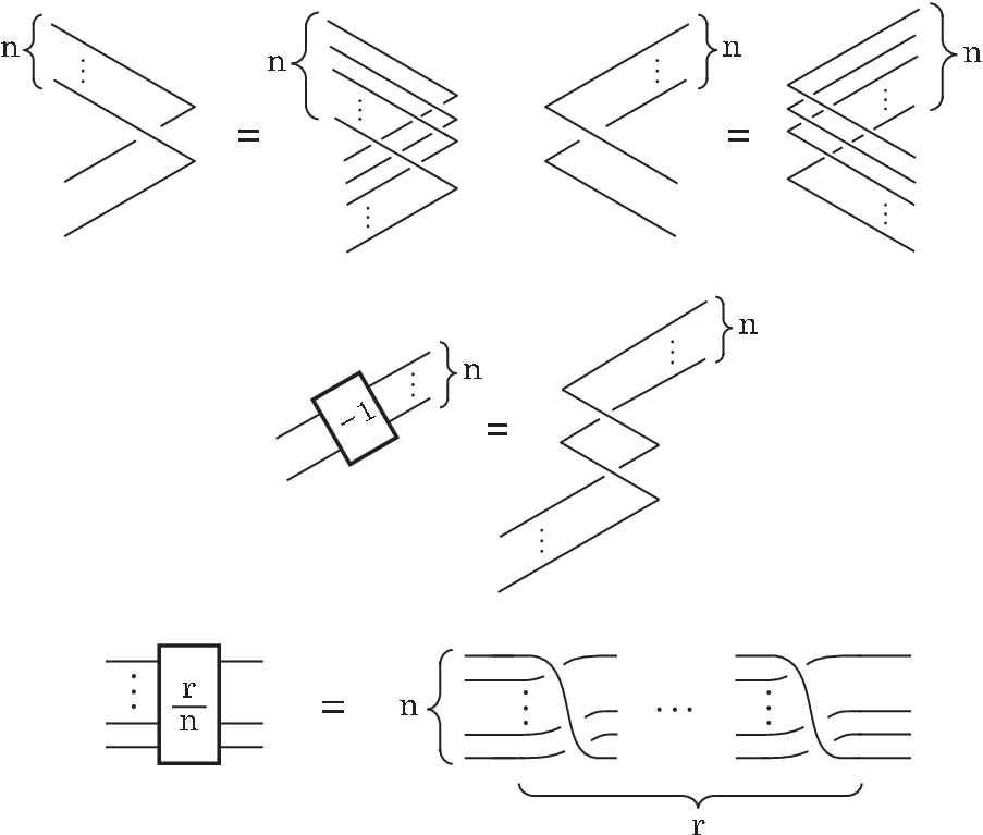
For a knot $K$ in the boundary of a 1-handlebody, a Legendrian knot $\mathcal{K}$ in the boundary is called a Legendrian representative of $K$, if $\mathcal{K}$ satisfies the condition below.

• •

  In the case where $K$ is homologically trivial, $\mathcal{K}$ is smoothly isotopic to $K$.

• •

  In the case where $K$ is homologically non-trivial, $\mathcal{K}$ is smoothly isotopic to $K$ without sliding $\mathcal{K}$ “over” any 1-handle. More explicitly, this condition is stated as follows. Consider the dotted circle notation of the 1-handlebody. The condition is that $\mathcal{K}$ is isotopic to $K$ by an isotopy of $S^{3}$ fixing the disks bounded by the dotted circles. Note that this condition does not allow slidings over the dotted circles.

We use this narrow definition to define the maximal Thurston-Bennequin number for a homologically non-trivial knot. The maximal Thurston-Bennequin number $\overline{tb}(K)$ of a knot $K$ in the boundary of a 1-handlebody is defined to be the maximal value of $tb(\mathcal{K})$ of a Legendrian representative $\mathcal{K}$ of $K$.

We remark that, if we change our narrow definition of a Legendrian representative to the natural one, then there are many examples of homologically non-trivial knots with $\overline{tb}=\infty$.

To see effectiveness of our method, we here estimate $\overline{tb}(K_{m,n})$ by the standard cabling construction of a Legendrian representative (cf. Section 5 in [7]). Before discussing the $(n,-1)$ cable $K_{m,n}$, we discuss its companion $K_{m}$. Since $K_{m}$ bounds a disk in $D^{4}$, the adjunction inequality shows $\overline{tb}(K_{m})\leq-1$. On the other hand, for $m\leq-1$, we can easily check that $K_{m}$ is isotopic to the Legendrian knot $\mathcal{K}_{m}$ with $tb=-1$ shown in Figure 4. Therefore, this Legendrian representative of $K_{m}$ realizes $\overline{tb}(K_{m})=-1$.

We draw $n$ copies of the front diagram of $\mathcal{K}_{m}$ each of which is slightly shifted to the vertical direction. Inserting $\frac{n-1}{n}$ right handed full twists to the resulting diagram appropriately, we obtain the Legendrian representative of $K_{m,n}$ in Figure 5. Calculating the number of left cusps and the writhe, one can easily check that $tb$ of this representative is $-2n+1$. Thus the standard construction merely shows $\overline{tb}(K_{m,n})\geq-2n+1$. It seems difficult to realize a larger Thurston-Bennequin number by modifying this representative.

Now we apply our method to $K_{m,n}$. We give necessary definitions to proceed Step 1 of the method. For an integer $m$, let $Z^{(m)}$ be the 4-manifold shown in Figure 6. Since the 2-handle goes over the 1-handle geometrically once after isotopy, $Z^{(m)}$ is diffeomorphic to $D^{4}$. We identify the boundary $\partial Z^{(m)}$ with $S^{3}$ via this diffeomorphism. Let $\widetilde{K}_{m}$ and $\widetilde{K}_{m,n}$ be the unframed knots in $\partial Z^{(m)}=S^{3}$ given by Figures 7 and 8, respectively.

To apply Step 1, we show the lemma below.

We regard $\widetilde{K}_{m,n}$ as a knot in the boundary of the sub 1-handlebody $Z^{(m)}_{1}$ of $Z^{(m)}$. Then $\widetilde{K}_{m,n}$ is clearly an unknot in the boundary $\partial Z^{(m)}_{1}$, and we know a Legendrian representative of an unknot realizing $\overline{tb}$. Therefore we finished Step 1.

Next we apply Step 2. We note that, if the framing $m$ of the 2-handle of $Z^{(m)}$ is a sufficiently large negative number, then we can obviously achieve this step. We first isotope $\widetilde{K}_{m,n}$ to its Legendrian representative realizing $\overline{tb}$ in $\partial Z^{(m)}_{1}$, and then we keep track of the 2-handle of $Z^{(m)}$ as shown in Figure 10. By putting the 2-handle into a Legendrian position, we obtain the Legendrian representative of $\widetilde{K}_{m,n}$ in $\partial Z^{(m)}_{1}$ shown in Figure 11 for $m\leq-4n+3$. Note that $Z^{(m)}$ is now a Stein handlebody and that $tb(\widetilde{K}_{m,n})=-1$. The Legendrian representative of $\widetilde{K}_{m,n}$ thus gives a Legendrian representative of ${K}_{m,n}$ in the boundary $\partial Z^{(m)}$ of the Stein handlebody, since $\widetilde{K}_{m,n}$ represents $K_{m,n}$ in $\partial Z^{(m)}$.

Since $\widetilde{K}_{m,n}$ bounds a disk in $Z^{(m)}_{1}$, the adjunction inequality shows $\overline{tb}(K_{m,n})\leq-1$. Therefore the Legendrian representative of $K_{m,n}$ in Figure 11 realizes $\overline{tb}=-1$. Note that this value of $\overline{tb}$ is equal to the one induced from the front diagram of $S^{3}$ (see Remark 3.2). This completes Step 2, and the proposition below follows.

Now we can easily prove Theorem 1.3.

Finally we apply Step 3 to obtain a Legendrian representative of $K_{m,n}$ realizing $\overline{tb}$ in the front diagram of $S^{3}$. We first apply local isotopies in Figure 14 to the Stein handlebody diagram of $Z^{(m)}$ and the knot $K_{m,n}$. Note that these isotopies preserve $tb$ of $K_{m,n}$ and the 2-handle. To simplify the diagram, we use tangles $A$ and $B$ defined in Figure 15. The resulting diagram of $K_{m,n}$ and $Z^{(m)}$ is shown in the first diagram of Figure 16. Now we can easily isotope the 2-handle and $K_{m,n}$ so that the 2-handle goes over the 1-handle geometrically once and that $tb$ of these knots do not change. The resulting diagram is given in the second diagram of Figure 16 (This isotopy can be easily seen by ignoring $K_{m,n}$ and tangles $A$ and $B$.).

Next we slide $K_{m,n}$ over the 2-handle so that $K_{m,n}$ does not go over the 1-handle (after suitable isotopy) and that $tb(K_{m,n})$ does not change. More specifically, we slide $K_{m,n}$ at the right most part of Figure 16 as shown in Figure 17, where the framings of the 2-handle are the contact $-1$ framings. We can easily check that this operation preserves $tb(K_{m,n})$ by counting the numbers of positive crossings, negative crossings and left cusps. Clearly we can isotope the resulting $K_{m,n}$ preserving $tb$ so that it does not go over the 1-handle. Now we can cancel (erase) the canceling pair of 1- and 2-handles. The resulting diagram is given in Figure 19, where we use the tangles $A_{n},B_{n}$ defined in Figure 18. Therefore, this diagram gives a Legendrian representative of $K_{m,n}$ realizing $\overline{tb}=-1$ in the front diagram of $S^{3}$. We thus completed Step 3.

As we mentioned in Remark 3.1, our method is also effective for finding a good lower bound of $\overline{tb}$ by minor modification. We demonstrate this using the knot $K_{m,n}$ with $n\geq 2$ and $m\leq-2n-1$.

Recall that $K_{m,n}$ is isotopic to the unframed knot $\widetilde{K}_{m,n}$ in the boundary of the handlebody $Z^{(m)}$ shown in Figure 8. We regard $\widetilde{K}_{m,n}$ as a knot in the boundary of the sub 1-handlebody $Z^{(m)}_{1}$ of $Z^{(m)}$. Since $\widetilde{K}_{m,n}$ is an unknot in $\partial Z^{(m)}_{1}$, we can isotope $\widetilde{K}_{m,n}$ to its Legendrian representative with $tb=-n+1$. We then isotope the 2-handle of $Z^{(m)}$ to its Legendrian representative fixing the representative of $\widetilde{K}_{m,n}$. The resulting diagram of $\widetilde{K}_{m,n}$ and $Z^{(m)}$ is shown in Figure 20. Clearly this diagram gives a Stein handle decomposition of $Z^{(m)}$, and thus the Legendrian representative of $\widetilde{K}_{m,n}$ gives a Legendrian representative of $K_{m,n}$ with $tb=-n+1$ in the Stein fillable contact structure on $\partial Z^{(m)}\cong S^{3}$. Hence the proposition below follows.

It seems difficult to obtain this estimate without using a handlebody diagram of $D^{4}$. We remark that we can also draw a Legendrian representative with $tb=-n+1$ in the front diagram of $S^{3}$, similarly to Step 3.

Characterizing an unknot is a natural question in knot theory, and various characterizations are known. Here we propose the following question as a potential characterization given by maximal Thurston-Bennequin numbers. Recall that $C_{p,q}(K)$ denotes the $(p,q)$-cable of a knot $K$ in $S^{3}$.

We remark that, for each positive integer $N$, Proposition 4.2 implies the existence of a non-trivial knot $K$ satisfying $\overline{tb}(C_{p,-1}(K))=-1$ for any positive integer $p\leq N$.

References

- [1] S. Akbulut and R. Matveyev, Exotic structures and adjunction inequality, Turkish J. Math. 21 (1997), no. 1, 47–53.
- [2] Y. Eliashberg. Topological characterization of Stein manifolds of dimension , International J. of Math. Vol. 1 (1990), No 1 pp. 29-46.
- [3] Y. Eliashberg. Filling by holomorphic discs and its applications, Geometry of low-dimensional manifolds, 2 (Durham, 1989), 45–67, London Math. Soc. Lecture Note Ser., 151, Cambridge Univ. Press, Cambridge, 1990.
- [4] Y. Eliashberg, Contact 3 -manifolds twenty years since J. Martinet’s work, Ann. Inst. Fourier (Grenoble) 42 (1992), no. 1-2, 165–192.
- [5] R. Fintushel and R. J. Stern, Immersed spheres in 4-manifolds and the immersed Thom conjecture, Turkish J. Math. 19 (1995), 145–157.
- [6] D. Fuchs and S. Tabachnikov, Invariants of Legendrian and transverse knots in the standard contact space, Topology 36 (1997), no. 5, 1025–1053.
- [7] M. Golla, Ozsváth-Szabó invariants of contact surgeries, Geom. Topol. 19 (2015), no. 1, 171–235.
- [8] R. E. Gompf, Handlebody construction of Stein surfaces, Ann. of Math. (2) 148 (1998), no. 2, 619–693.
- [9] R. E. Gompf and A. I. Stipsicz, -manifolds and Kirby calculus, Graduate Studies in Mathematics, 20. American Mathematical Society, 1999.
- [10] F. Gonzalez-Acuna and H. Short, Knot surgery and primeness, Math. Proc. Cambridge Philos. Soc. 99 (1986), no. 1, 89–102.
- [11] C. McA. Gordon, and J. Luecke, Only integral Dehn surgeries can yield reducible manifolds, Math. Proc. Cambridge Philos. Soc. 102 (1987), no. 1, 97–101.
- [12] J. E. Greene, L-space surgeries, genus bounds, and the cabling conjecture, J. Differential Geom. 100 (2015), no. 3, 491–506.
- [13] P. Kronheimer and T. Mrowka, The genus of embedded surfaces in the projective plane, Math. Res. Lett. 1 (1994), no. 6. 797–808.
- [14] T. Lidman and S. Sivek, Contact structures and reducible surgeries, arXiv:1410.0303, to appear in Compositio Math.
- [15] P. Lisca and G. Matić, Tight contact structures and Seiberg-Witten invariants, Invent. Math. 129 (1997) 509–525.
- [16] P. Lisca and G. Matić, Stein 4-manifolds with boundary and contact structures, Topology and its Applications 88 (1998) 55–66.
- [17] J. Morgan, Z. Szabó and C. Taubes, A product formula for the Seiberg-Witten invariants and the generalized Thom conjecture, J. Differential Geom. 44 (1996), 706–788.
- [18] L. Ng, A Legendrian Thurston-Bennequin bound from Khovanov homology, Algebr. Geom. Topol. 5 (2005), 1637–1653.
- [19] L. Ng, On arc index and maximal Thurston-Bennequin number, J. Knot Theory Ramifications 21 (2012), no. 4, 1250031, 11 pp.
- [20] B. Ozbagci and A I. Stipsicz, Surgery on contact 3-manifolds and Stein surfaces, Bolyai Society Mathematical Studies, 13. Springer-Verlag, Berlin; Janos Bolyai Mathematical Society, Budapest, 2004.
- [21] P. Ozsváth and Z. Szabó, The symplectic Thom conjecture, Ann. of Math. 151 (2000), 93–124.
- [22] P. Ozsvath and Z. Szabo, Knot Floer homology and the four-ball genus, Geom. Topol. 7 (2003), 615–639.
- [23] O. Plamenevskaya, Bounds for the Thurston-Bennequin number from Floer homology, Algebr. Geom. Topol. 4 (2004), 399–406.
- [24] O. Plamenevskaya, Transverse knots and Khovanov homology, Math. Res. Lett. 13 (2006), no. 4, 571–586.
- [25] J. Rasmussen, Khovanov homology and the slice genus, Invent. Math. 182 (2010), no. 2, 419–447.
- [26] A. Shumakovitch, Rasmussen invariant, slice-Bennequin inequality, and sliceness of knots, J. Knot Theory Ramifications 16 (2007), no. 10, 1403–1412.
- [27] K. Yasui, Nonexistence of Stein structures on 4-manifolds and maximal Thurston-Bennequin numbers, arXiv:1508.01491, to appear in J. Symplectic Geom.