New Parities and Coverings over Free Knots
Abstract
In the present paper, we develop the parity theory invented in [12]; we construct new parities for two-component (virtual and free) links. New parities significantly depend on geometrical properties of diagrams; in particular, they are mutation-sensitive.
New parities can be used practically in all problems, where parities were previously applied.
Keywords: Knot, link, virtual knot, virtual knot, virtual link, free knot, free link, parity.
1 Introduction
The theory of multi-component links is much richer than the theory of knots. Thus, for classical links there exists a powerful link-homotopy theory [14, 5]: the simplest link homotopy invariant is the linking coefficient. Classical invariants of knots can be modified if one passes from knots to multicomponent links.
Virtual knot theory invented by Kauffman [6] includes classical knot theory. As it turns out, the behaviour of one-component virtual knots is similar to the behaviour of classical links; virtual knots admit invariants similar to invariants of multicomponent classical links. Thus, in [7] the “self-linking coefficient” for virtual knots was defined.
This effect is possible because of parities and coverings over virtual knots: there exists a well defined map from the set of virtual knots to the set of virtual links.
The parity theory invented by the author [12], see also [4, 13], allows one to make a distinction between two types of crossings of virtual knots, even ones and odd ones (in fact, this can be done even for a simplification of virtual knots called free knots); this circumstance allows one to treat virtual knots as multicomponent links by means of coverings coming from parities. These coverings were first used in [11] for the construction of Khovanov homology theory for virtual knots.
Usually, knot invariants are valued in some algebraic objects: numbers, polynomials, groups. The information about knots encoded by such invariants is very implicit. Say, a grading or a degree of some knot invariant allows one to judge about the crossing number of a knot, but not about the geometrical form of diagrams of the knot. The algebraic nature of invariants allows one to construct easily some transformation which do not change the values of the invariant, but change the knot dramatically.
For an important example one can take mutations, [3]. Mutations change the topology of the knot dramatically but do not affect the value of most of algebraic invariants.
The parity theory allows one to construct knot invariants valued in knot diagrams, which allows one to solve problems of the following sorts:
- 1.
Reduce properties of knots to properties of their diagrams;
- 2.
Construct functorial mappings between knots.
Particularily, the first problem can be solved by using the so-called “parity bracket” introduced by the author in [12]. This parity bracket is a well defined map from the set of knots to the set of graphs; if some “oddness” and “irreducibility” conditions are satisfied, then the bracket of a free knot diagram is equal to the diagram itself.
The first statement can be formulated as the following “meta”theorem
Theorem 1.
If a (virtual) knot diagram is complicated enough (“odd”) then any diagram equivalent to it contains as a subdiagram.
View Fig. 1. This figure demonstrates how the theorem applies to a unique second Reidemeister move applied to the diagram .

Among parities, the Gaussian parity plays a special role. It is the only non-trivial parity for free knots. This parity is also defined for knotted spheres (see [13]), which are smoothly mapped to -manifolds. A formal definition in [13] was given for discs, but it can be generalized verbatim for the case of spheres. Thus, the Gaussian parity allows one to construct not only invariants of free knots but also a sliceness obstruction: an obstruction to span a free knot by a disc with standard “-dimensional” singularities.
The other parities for knot theories require some additional structure defined on knots/links; there is no such general structure for free knots.
The major part of invariants constructed by the author in previous papers (for references, see [9, 4]) are well defined for any parity.
However, the parities themselves for knot theories can be constructed easily by looking at some combinatorial or homological properties. Parities that we are going to construct in the present paper are based on some “patterns” (subdiagrams) in a given diagram. This means that some crossing of a knot diagram is decreed even or odd depending on whether there exist some “subknots” inside the knot located in a predicted manner with respect to the given crossing. This makes parity arguments even more delicate.
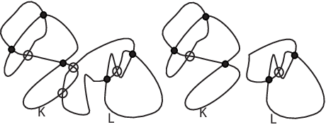
In Fig. 2, we schematically show a way of changing a link or its component (say, mutation); together with its pattern in question ; such a transformation will not change “algebraic” invariants whose construction is based on some “bare count“; however, such an effect can be tackled by looking at parities based on patterns.
The new parities are based on some count of intersections with a given pattern .

Thus, if the sample changes slightly as shown in Fig. 2, then the parity changes drastically. For example, the right part of Fig. 2 does not contain at all, so all the crossings are even, whereas some crossings in the left part of the figure are odd.
Let us note that various topological constructions of parity theory lead us to “graphical” results in classical knot theory, see [2, 8, 1].
In the present paper, we shall show how to construct various new parities for the two-fold covering over a free knot, where the two-fold covering is constructed by using the Gaussian parity, and how to use these new parities to construct new invariants of free knots.
In the sequel, we are planning to use new parities in order to construct invariants of free knot cobordisms.
The present paper is organized as follows.
In the second section, we give the definition of free knots, known parities, the parity bracket, and present a detailed discussion of the Turaev delta (also known as Turaev’s bracket) as well as a detailed discussion of the two-fold covering over virtual knots.
In the third section, we define the parity for crossings of one component in a two-component link and show that in the case of a two-component link, the bracket and the delta may lead one to more elaborated parities.
The last section is devoted to the construction of various examples illustrating various subtleties of new parities and invariants coming from them.
1.1 Acknowledgements
The present work is supported by the Laboratory of Quantum Topology ot the Chelyabinsk State University (Russian Govenrment Grant No, ; 14.Z50.31.0020)
I am deeply indebted to I.M.Nikonov for various discussions of various (Russian and English) versions of the text; I am also grateful to D.P.Ilyutko, D.A.Fedoseev, and V.A.Krasnov for fruitful discussions.
I am also grateful to the referee for various remarks concerning the text.
2 Basic definitions
2.1 Free knots and links
Definition 1.
By a -graph we mean a -dimensional complex each component of which being either homeomorphic to the circle or being a four-valent graph; by vertices of a -graph we mean vertices of its components which are not homeomorphic to circles; by edges of a -graph we mean edges of its components which are not homeomorphic to circles as well as components homeomorphic to the cirlce (the latter will be called cyclic components or cyclic edges); every non-cyclic edge will be treated as an equivalence class of the two (different!) half-edges composing it.
Remark 1.
Note that the CW-structure is immaterial in the sequel; we assume that there are no vertices on cyclic edges.
Definition 2.
We say that a -graph is framed, if at each vertex of this graph, the four half-edges are split into two pairs of opposite ones; we shall call such a splitting a framing; half-edges which are incident to the same vertex and are not opposite, will be called adjacent. Framed -graphs are considered up to the natural equivalence, i.e., a homeomorphism which preserves the framing (we do not impose any restrictions on cyclic components).
Remark 2.
In the sequel, we treat framed -graphs only up to equivalence.
By a cyclic universal component of a framed -graph we mean an equivalence class of edges of this graph containing only one cyclic edge.
Remark 3.
When drawing framed -graphs on the plane, we shall not indicate the framing assuming that formally opposite half-edges are exactly those locally opposite on the plane. Framed -graphs appear naturally when considering generic immersions of a collection of circles into the plane; the framing is inherited from the immersion.
Homotopy classes of curves in -surfaces motivate the following set of elementary equivalences on framed -graphs called Reidemeister moves, see Fig. 3.
When drawing diagrams on the plane, we will show only their changing parts (e.g., for moves).
Definition 3.
By a free link [12] we mean an equivalence class of framed -graphs modulo Reidemeister moves.
Definition 4.
By an orientation of a free link we mean orientations of all its cyclic components together with orientation of all edges belonging to non-cyclic components in such a way that for each two edges which are incident to the same vertex and opposite ate this vertex, one is incoming and the other one is emanating.

We say that a Reidemeister move is increasing, if it increases the number of vertices and decreasing if it decreases the number of vertices.
By a non-cyclic unicursal component of a framed -graph we mean an equivalence class of its edges generated by the elementary equivalence: two edges are elementary equivalent if they are opposite at some vertex.
One naturally gets (see [12]) the number of unicursal components of a free link.
Each crossing of a free link belongs either to one unicursal component or to two different components. In the former case, we shall call it the pure crossing, in the latter case, the crossing is mixed.
If a crossing of a framed -graph is not mixed then the unicursal component passing through this crossing is naturally split into two halves. We say that the two edges belonging to one unicursal component belong to the same half if there exists a chain of edges where every two adjacent edges are opposite at some vertex distinct from . In Fig. 4, chords of the chord diagram corresponding to one half with respect to the vertex , are denoted by , and chords of the other half are denoted by .

We say that a (-component) link is splitting if it can be represented by a splitting diagram; a (-component) diagram, in turn, is splitting if it has no mixed classical crossings.
In Fig. 5, both diagrams are splitting ones. The diagram on the LHS is splitting because it has no pure classical crossings; the diagram on the RHS has no mixed crossings at all; those “virtual crossings” depicted by circles are not counted as vertices.
Remark 4.
Generically, diagrams of curves on two-surfaces, carry more information than framed -graph. To a framed -graph, there corresponds many different immersions into surfaces (even if we restrict ourselves to connected -graphs and even if we require that the graph tiles the surface into cells)). Thus, there is a natural “forgetful” map from homotopy classes of classes of curves on -surfacest to framed -graph.
This map exactly corresponds to the forgetful map from flat links to free links.
2.2 The Parity. The Gaussian Parity
Assume some class of knots represented by equivalence classes of diagrams modulo moves is given; the diagrams are required to be framed -graphs, possibly, with some additional structures and/or restrictions, and possibly, some additional restrictions are imposed on Reidemeister moves. Thus, classical knots can be thought of as planar diagrams modulo moves where edge cyclic structure together with ovepass/underpass structure is indicated, and natural restrictions are imposed on the second and the third Reidemeister moves.
Assume we are given a rule which assigns with each vertex of a diagram from the class a number (such vertices will be called even) or (in this case, the vertex is called odd). In the sequel, we shall denote the parity of a vertex by and write if the crossing is even and if the crossing is odd.
Definition 5.
We say that the above rule satisfies the parity axiomatics if the following holds. For every two diagrams and obtained from each other by one Reidemeister moves where has no more crossings than the following conditions hold:
- 1.
if is obtained from by the first Reidemeister move, then the crossing of participating in the Reidemeister move, is even;
- 2.
if is obtained from by the second Reidemeister move, then both crossings taking part in the Reidemeister move have the same parity;
- 3.
if is obtained from by the third Reidemeister move, then there exists a natural correspondence between the triple of crossings of and the triple of crossings of taking part in the Reidemeister moves(), see Fig. 6.

Figure 6: The third Reidemeister moves and corresponding crossings We require that
a) ,
b) among , the number of odd crossings is even (i.e., equals or ).
- 4.
We require that those crossings which remain untouched when passing from , preserve their parity.
Remark 5.
If a framed -graph admits a symmetry (i.e., a framing-preserving isomorphism), then it follows from the definition that this symmetry preserves the crossing parity.
As an example, let us define the Gaussian parity, as follows.
Definition 6.
A chord diagram is a regular -graph consisting of a selected non-oriented Hamiltonian cycle (the core) of the chord diagram and non-oriented edges (chords),, where each chord connects some two points on the circle, in such a way that different chords do not share points on the circle.
We say that two chords are linked, if the endpoints of one of them belong to different connected components of the set obtained from by deleting the endpoints of the other chords. Otherwise, the chords are called unlinked.
We shall also admit the empty chord diagram, i.e., the chord diagram without chords which is formally not a graph..
Remark 6.
Analogously, one considers multichord diagrams or chord diagrams on several circles.
Definition 7.
A chord of a chord diagram is even (with respect to Gauss) is the number of chords, it is linked with, is even. Otherwise, we call this chord odd. A vertex of a framed -graph is even or odd depending on whether the corresponding chord of the chord diagram is even or odd.
Finally, we say that a chord diagram is even if all chords of it are even and odd if all chords of it are odd.
If a framed -graph has one unicursal component, then it can be thought of as the image of the map , which is bijective everywhere outside neighbourhooods of vertices of and their preimages.
Thus, framed -graphs we are interested in are encoded by chord diagrams, and chords correspond to vertices.
In Fig. 7, we show a framed -graph and the chord diagram corresponding to it.

Absolutely analogously, one can define the correspondence between framed -graphs on many components and multichord diagrams (chord diagrams on many circles).
If we deal with multicomponent chord diagrams, parity can be defined only for pure crossings.
Definition 8.
We say that a vertex of framed chord diagram is even (with respect to Gauss) if the corresponding chord of the chord diagram is even, and odd, otherwise.
In other words, one can define the parity of a vertex (we deal with a free knot) of a framed -graph as the parity of the number of crossings (common vertices) between the two halves of formed by .
It can be easily seen that for free knots, the Gaussian parity satisfies all parity axioms.
In [4] it is proved that the Gaussian parity is the only parity for free knot. Parities for free links are also classified there.
The aim of the present paper is to find non-trivial “parities” which correspond to pure crossings of a free link only, provided that a link has a second component. From the formal point of view, this parity is not a parity for two-component links since it is defined not for all crossings; however, as we shall see further, there will be infinitely many parities of such sort, moreover, non-trivial free knot homotopy type will lead to such parities by means of “patterns”, and these parities will depend on “geometry” of both components.
2.3 The Bracket and The Delta
In the present section we recall the two important mapping for free knots, the parity bracket, see [12], and the Turaev Delta, see Fig. [15].
The first one gives an invariant of free knots valued in linear combinations of framed -graphs.
The second one is a mapping from free knots (with one component) to free links (with two components).
For each framed -graph with a non-empty set of vertices, for each vertex , we define the two splittings ,, both being framed -graphs.
An even splitting is a splitting performed at one or several even crossings.
Let us define the linear space as the set of -linear combinations of the following objects. We consider all framed -graphs modulo the following equivalence relations:
1) the second Reidemeister move;
2) , i.e., the framed -graph having more than one component with at least one trivial component, is assumed to be equal to zero.
Denote by the linear subspace of the space generated by framed -graphs with a unique unicursal component.
Remark 7.
One can easily see that the equivalence classes listed below are uniquely characterized by their minimal representatives, i.e., framed -graphs without single circles and bigons. Thus, for summands from and , we shall use the term “graph” assuming some minimal element of the corresponding equivalence class.
There exists a natural map , taking all equivalence classes of framed graphs with more than one unicursal component, to zero. It is evident that is a group epimorphism.
Let be a framed-graph such that each unicursal component of has evenly many edges. In particular, the construction given below will work for the case of free knots: if we have exactly one component then all edges belong to it.
The invariant (see [12]) is given by
where the sum is taken over all even smoothings of the framed -graph , which are considered as elements of the group .
Here by an even smoothing we mean a smoothing at all even crossings.
Theorem 2.
The bracket is an invariant of free links.
The bracket is defined for free knots and is obtained by projecting the bracket to the subspace ; in other words,
Let us now modify the bracket as follows. We shall consider the two-component free links and apply the smoothings to even crossings of the second component, i.e., we set
where the sum is taken over all even smoothings of the framed -graph having one component.
We shall get a collection of graphs having two components each: one component is exactly the component , and the other component is depending on the state . By looking at components , one can construct further parities of the component .
2.3.1 The map (Turaev’s cobracket [15])
We shall construct a map from -linear combinations of oriented free knots to -linear combinations of oriented non-split free links.
Given an oriented framed graph , and let be the crossings of . At each crossing there is a unique way of smoothing for respecting the orientation: ; we shall denote the result of smoothing by . Thus, we can define a map
| (1) |
where the sum is taken over those crossings for which the link is non-split.
The restriction above on is imposed for the map to be well defined: if we apply the first increasing Reidemeister move to , then on the RHS of (1) we shall get split links with trivial components as additional summands.
Thus, in order to get a well defined delta (cobracket), one should weaken some conditions, and forbid not all split summands, but only those where one component is trivial.
The invariance of delta under the second and the third moves is checked straightforwardly, see [12].
Among the summands (1), one can naturally take only those where the resulting links looks very specially (e.g., one component represents some concrete free knot).
Analogously, one can define maps from -component free links to -linear combinations of -component free links, where the corresponding sum is taken only over those crossings lying in one component, with some additional restrictions and factorizations.
In the sequel, we shall need various modifications of the map to get free links and free knots and to construct parities.
2.4 The projection and the twofold covering
Each parity in a knot (link) theory induces two natural maps (projection and a twofold covering) that are constructing in the following way.
Let be a framed -graph. We construct graphs and as follows. Firstly, assume that the graph is connected.
If is a cycle, then the graph consists of one cycle and the graph consists of two cycles of the same length. We say that the cycles of are dual to each other and that they cover the cycle of .
To each vertex of the graph we assign two covering vertices . These vertices will be called dual. Choose a spanning tree of the graph .
We call all the edges of to be good. Edges of which do not belong to are divided into good and bad edges as follows. Any edge in connects vertices and determines in a minimal cycle which consists of the edge and the shortest path from to in the tree. This cycle is rotating (from an incident edge to a neighbouring edge) at some vertices and transversal at the remaining vertices. We call the edge good if the number of transversal vertices in the cycle is even.
To each edge of the spanning tree , which connects two vertices , we assign two covering edges , where the edge connects with . We shall call the edges and dual.
We do the same with the good edges which do not belong to the spanning tree .
To each bad edge , which connects the vertices and , we assign two covering edges , the first edge connects and , the second edge connects and . The edges will be called dual.
Let be the constructed graph. The framing of a vertex of is naturally induced from the graph which is covered by . One checks directly that the constructed graph and the duality relation do not depend on the choice of the spanning tree.
If is not connected, then the graph is constructed as the split sum of the graphs that correspond to the connected components of the graph .
There is a natural involution on the graph that maps each vertex to the dual vertex and each edge to the dual edge. Since the duality is compatible with the framing relation at a vertex, there is a natural definition of dual components of .
The diagram can be obtained from by removing one of the two sets of components.
The following statement can be checked straightforwardly.
Theorem 3.
[12] The maps are well defined, i.e., when applying the Reidemeister move to the diagram , the diagrams are operated on by combinations of Reidemeister moves.
Remark 8.
In the case if contains of a unique component, the map is described as follows. The chord diagram is obtained from by deleting all odd chords.

An example of the covering over a framed -graph is shown in Fig. 8.
The graph shown in Fig. below, has two vertices and . For the spanning tree , we shall take the tree consisting of one edge and two vertices ,. The remaining edges will also connect to . Herewith, the edge is good, and the edges and are bad. In the upper part of Fig. 8, we show the orientation at vertices and , which agrees along the edge .
This orientation is well defined on the edge but disagrees with itself along and . The cycle is good since it rotates at one vertex and is not transverse anywhere, and both cycles are bad (each of them is transverse at some vertex).
3 Parities relative to a component of a free link
The first known parity was the Gaussian parity. It was defined on free knots and virtual knots and it is the only non-trivial parity for free knots.
We shall see below that for two-component links one can define a similar parity for one component (for crossings of the other component the parity is not defined).
If we want to combine such a parity with the covering map, we construct for a knot its covering and get the parity on the crossings of the diagram relative to the diagram . Since the crossings of the diagram come from the even crossings of the diagram the even crossing of split into two types. This construction was essentially described in [13] where one discusses the “refined parity” of even crossings in a diagram which contains both even and odd crossings.
Nonetheless, that refined parity is based on calculation of intersections in the diagram.
In Fig. 2 we have demonstrated how to construct rather elaborated parities for one component of a free knot by using sample subdiagrams.
It appears that by combining covering approach and the new parities for one component of two-component link relative to the other component, we can get very non-trivial parities for crossings of a component in the link obtained as the covering of a diagram .
Such parities allow one immediately to construct and refine various invariants of the initial diagram , whose values depend on the presence of one or another sample.
3.1 Definition. The Simplest Example
Let be a two-component free link with evenly many mixed crossings.
Let us call a third Reidemeister move of the link special if it involves one crossing of the component and two mixed crossings (of the component with the component ).
Definition 9.
Let be a rule which for some class of free links assigns a number equal or to each crossing of the component . We call parity for in if the following axioms hold:
a) usual parity axioms (see Definition 5) for the Reidemeister moves which involve only crossings of the component ;
b) Reidemeister moves which involve crossings of the component or mixed crossings do not change parity of the crossings of (see Fig. 9);
c) any special third Reidemeister move does not change the parity of the crossing of the component .

For each crossing of the component we define the parity as the parity of number of mixed crossings in a half (the choice of the half does not matter).
Theorem 4.
is a parity for in .
The statement follows from the straightforward check of Reidemeister moves.
Example 1.
Let us consider the following two-component link . It has one pure crossing belonging to the component and two mixed crossings and ; one of them belongs to one half of with respect to , and the other one belongs to the other half of with respect to .
According to the definition, the crossing is the only odd crossing of the link diagram.
It follows from the definition that for any other diagram of the link , the component also contains an odd crossing. These arguments yield the minimality of the diagram shown in Fig 10.

3.2 Parities obtained from Turaev’s cobracket
The parity considered above for one component, being relative to the other component, like the Gaussian parity, is defined by an arithmetic calculation of crossings of some type. It appears that one can construct parities which depend on the presence of some “sublink” in the given link. For this we apply some operation (delta or bracket) to the component of a two-component link and look how the result of the operation intersects the component .
Let us describe the parity construction in more detail.
The first parity will depend on some link , the presence of the link as a resolution of the diagram means all the crossings of the diagram are odd.
Let be a free non-splittable two-component link whose component and are not trivial and are not equivalent to each other.
Let be the set of equivalence classes of non-splittable free three-component links and let be the corresponding free module.
We consider a map which relates ordered two-component links with an element of the module . This map is the composition of two maps: .
Here is the ordered map which maps two-component links to –linear combinations of three-component links. This map relates a link to the sum , where the resolution is taken for all pure crossings of the diagram , and we do not consider splittable summands ; as a result we get a linear combination of three-component links with a distinguished component .
By applying the projection , we keep only those summands for which the two-component link obtained from is equivalent to . Since and are not equivalent the components of each summand can be ordered so that the first component is , the second component is and the third component is .
Statement 1.
The map is well defined.
The statement follows from the direct check of Reidemeister moves.
Let us define the parity for the knot relative to in the link .
Let be a link with even number of mixed crossings. Each pure crossing of the component of the link corresponds naturally to a crossing in every term in the sum . We denote this crossing as as well. One can consider the two-component sublink and the parity relative to the component equivalent to . Summing these parities for all the summands of the sum , we get the number .
Statement 2.
For links with even number of mixed crossings, the parity is a well-defined parity for relative to .
Proof.
For all Reidemeister moves except for a second move applied to the component the number of summands in does not change, one can identify all crossings of in every summand, and the corresponding parities do not change.
A second move on the component leads to two new summands. Their contributions into the parity for each crossing of the diagram annihilate, see Fig. 11.
The figure shows two diagrams that differ with a second Reidemeister move. Below the two contracting summands are shown.

∎
3.3 Parities obtained from the parity bracket
The idea of another parity construction is the following. Let be a two-component link and let the component be odd and irreducible. Consider as a four-valent graph and consider a basis of the homology group of the graph. Each element is presented as a cycle (or sum of cycles) in . Assume that each of these cycles has even number of intersections with the component .
Then we can call a crossing of the component of the diagram to be even (resp., odd) relative to if the intersection number of a component half at the crossing with the cycle is even (resp., odd).
Let us define a linear space as the set of –linear combinations of the following objects. We consider all framed 4-graphs with two ordered unicursal components modulo the following equivalence relations:
1) all possible Reidemeister moves for the first component and all possible mixed Reidemeister moves;
2) second Reidemeister moves on the component .
Remark 9.
Unlike , there is no obvious recognition algorithm for .
Let be the framed -graph with two ordered components and . Let us define the invariant according to the formula
where the sum is taken over all even splittings of the framed -graph having one component.
A straightforward Reidemeister move check leads us to the following
Theorem 5.
is an invariant of -component links with ordered components.
4 Further discussion
It turns out that this definition can be extended for a parity of the component in by using .
Let us now consider .
It turns out that in some special cases, for each diagram of the link , one can identify the homology classes which correspond to the classes of the diagram in such a way that the following holds:
Statement 3.
Let us consider two-component links possessing the above properties. Then the maps are well defined parities for the knot with respect to .
References
- [1] M. W. Chrisman. Knots in virtually fibered 3-manifolds ArXiv e-prints, May 2014
- [2] M. W. Chrisman and V. O. Manturov. Fibered knots and virtual knots. J. Knot Theory Ramifications, 22(12) (2013) :1341003, 23.
- [3] Peter R.Cromwell, Hugh R. Morton,: Distinguishing mutants by knot polynomials. J. Knot Theory Ramifications 5 (1996), no. 2, 225238.
- [4] D.P.Ilyutko, V.O.Manturov, I.M.Nikonov, Parity in Knot Theory and Graph-Links, Journal of Mathematical Sciences, September 2013, Volume 193, Issue 6, pp. 809–965.
- [5] N.Habegger, X.-S.Lin, (1990), The classification of links up to homotopy, Journal of the American Mathematical Society, 2 (American Mathematical Society) 3 (2): 389419
- [6] Kauffman L. H. Virtual knot theory// European Journal of Combinatorics. — 1999. — 20, No. 7. — Ñ. 663–690.
- [7] Kauffman L. H. A Self-Linking Invariant of Virtual Knots// Fundamenta Mathematicae. — 2004. — 184. — Ñ. 135–158.
- [8] V. A. Krasnov and V. O. Manturov. Graph-valued invariants of virtual and classical links and minimality problem. J. Knot Theory Ramifications, 22(12):1341006, 14, 2013.
- [9] V.O.Manturov and D.P.Ilyutko, Virtual Knots: The State of The Art (2013), World Scientific, Series on Knots and Everything, Vol. 51, Singapore.
- [10] V.O.Manturov, Long Virtual Knots and Their Invariants, J. Knot Theory Ramifications, Vol. 13 (8), 2004, P. 1029-1039, 2004.
- [11] V.O.Manturov, The Khovanov Complex for Virtual Links, Journal of Mathematical Sciences (New York), 2007, 144:5, 44514467
- [12] V.O.Manturov, Parity in Knot Theory, Sbornik: Mathematics, 2010, 201:5, 693733.
- [13] V.O.Manturov, Parity and Cobordisms of Free Knots, Sbornik: Mathematics, 2012, 203:2, 196223.
- [14] Milnor, J. Link Groups, Ann. Math., 59 (1954), pp. 177-195.
- [15] V. G. Turaev, Topology of Words, Proc. Lond. Math. Soc. 2007, 95:3, P. 360-412.