Low energy Lorentz violation from modified dispersion at high energies

Introduction. — Although local Lorentz invariance is a pillar of modern physics, there exist serious proposals emerging from quantum theories of spacetime that Lorentz invariance may be broken at sufficiently high energies [1]. The challenge for such proposals is twofold: to recover approximate Lorentz invariance in the well tested low energy regime, and to make predictions through which the violation could conceivably be observed.

If a Lorentz violating theory contains an explicit energy scale $M_{\star}$ that characterizes the violation, such as the Planck energy, it might seem straightforward to secure approximate Lorentz invariance at energies much below $M_{\star}$. However, in quantum field theory (QFT), the effective low energy theory can reveal unexpected imprints of the theory’s high energy structure [2]. For example, a Lorentz violation that is superficially associated with a large energy scale can become observable at arbitrarily low energies via the renormalization of a logarithmically divergent loop diagram [3]. There is a similar result for the Casimir effect [4].

The purpose of this paper is to show that such an unexpected low energy imprint occurs in the response of a simplified atom, modeled as an Unruh-DeWitt (UDW) detector [5, 6], coupled to a class of Lorentz violating quantum field theories in four-dimensional Minkowski spacetime.

The theories we consider have a dispersion relation which in the preferred frame reads

where $\mathbf{k}$ is the spatial momentum, $\omega_{|\mathbf{k}|}$ is the corresponding energy, the positive constant $M_{\star}$ is the energy scale of Lorentz violation, and $f$ is a smooth positive function on the positive real line, with the property that $f(x)\to 1$ as $x\to 0_{+}$. (We set $c=\hbar=1$.) This dispersion relation is approximately Lorentz invariant for $|\mathbf{k}|/M_{\star}\ll 1$.

Despite this low energy recovery of Lorentz invariance, we find that, for any $f$ that dips below unity somewhere, transitions in an inertial UDW detector are strongly Lorentz violating at arbitrarily low transition energies. If $f_{c}:=\inf f$ satisfies $0<f_{c}<1$, the signature of the violation is a sudden enhancement in the rate of spontaneous de-excitations and a sudden emergence of spontaneous excitations when the detector’s rapidity exceeds the critical value $\beta_{c}:=\artanh(f_{c})$. Crucially, $\beta_{c}$ is independent of $M_{\star}$.

As an application, we show that this class of Lorentz violating theories includes a scalar field quantized in the polymer quantization framework [7, 8, 9, 10, 11, 12], a method motivated by the loop quantum gravity (LQG) program [13, 14]. For the polymer quantized scalar field, we find that large Lorentz violation occurs above the critical rapidity $\beta_{c}\approx 1.3675$, a value well below $\beta\approx 3$ attained by ions at the Relativistic Heavy Ion Collider (RHIC) [15]. Given the close correspondence between the Unruh-DeWitt detector and an atom interacting with the electromagnetic field [16, 17], the absence of observations of Lorentz violation at the RHIC therefore provides a strong constraint on the possible families of modified dispersion relations.

Field theory with modified dispersion relation. — We consider a real scalar field $\phi$ that admits a decomposition into spatial Fourier modes such that a mode with spatial momentum $\mathbf{k}\neq\mathbf{0}$ is a harmonic oscillator with the angular frequency $\omega_{|\mathbf{k}|}$ (1), where $f$ is a smooth positive function on the positive real line. To allow sufficient generality, we will for the moment leave the small argument behaviour of $f$ unspecified, and we include in the Fourier decomposition the density-of-states weight factor

where $d$ is a smooth complex-valued function on the positive real line. If $f(x)=1$ and $d(x)=2^{-1/2}$, the field is the usual massless scalar field.

The central object that will be needed below is the Wightman function in the Fock vacuum. It is given by

where the distributional character is encoded in the limit $\epsilon\to 0_{+}$.

Model atom: UDW detector. — We probe the field with a linearly-coupled two-level UDW detector [5, 6]. This detector model captures the essential features of an atom interacting with the electromagnetic field [16, 17], and it has been widely used to analyze motion effects in quantum field theory (for recent reviews see [18, 19, 20]).

The detector is pointlike and moves on the worldline ${\sf{x}}(\tau)$ where $\tau$ is the proper time. The coupling strength is proportional to the switching function $\chi(\tau)$, which is non-negative and smooth, and falls off sufficiently rapidly at $\tau\to\pm\infty$. In first-order perturbation theory, the probability of the detector to make a transition from the state with energy $0$ to the state with energy $\Omega$ (which may be positive or negative) is then proportional to the response function, $\mathcal{F}(\Omega)=\int d\tau\,d\tau^{\prime}\,\chi(\tau)\chi(\tau^{\prime})\,e^{-i\Omega(\tau-\tau^{\prime})}\mathcal{W}(\tau,\tau^{\prime})$, where $\mathcal{W}$ is the pullback of the scalar field’s Wightman function to the detector’s worldline.

When both the trajectory and the quantum state of the field are stationary, $\mathcal{W}(\tau,\tau^{\prime})$ depends on its arguments only through the difference $\tau-\tau^{\prime}$, and we may convert $\mathcal{F}$ into the transition rate per unit time by passing to the limit of adiabatic switching and factoring out the effective total duration of the detection. While this procecure is subtle [19, 21, 22], for the present purposes we may consider the specific switching function family $\chi(\tau)=\pi^{-1/4}\sigma^{-1/2}\exp\bigl[-\tau^{2}/(2\sigma^{2})\bigr]$, where the positive constant $\sigma$ is the effective duration of the interaction, and the normalization factor $\sigma^{-1/2}$ provides the conversion from transition probability to transition rate. For finite $\sigma$ the transition rate is given by $\mathcal{F}(\Omega)=\int_{-\infty}^{\infty}ds\,e^{-s^{2}/(4\sigma^{2})}\,e^{-i\Omega s}\,\mathcal{W}(s,0)$. Passing to the limit in which $\sigma$ is large compared with $1/|\Omega|$ and with the timescales over which $\mathcal{W}$ varies, we obtain

We shall use equation (4) in the analysis that follows.

Inertial detector. — We consider a detector on the inertial worldline $\bigl(t(\tau),\mathbf{x}(\tau)\bigr)=\bigl(\tau\cosh\beta,0,0,\tau\sinh\beta\bigr)$, where $\beta$ is the rapidity with respect to the distinguished inertial frame. For presentational simplicity we proceed assuming $\beta>0$, but it can be verified by a separate analysis that the $\beta=0$ transition rate is equal to the $\beta\to 0$ limit of the results given below.

From (3) and (4) we obtain

where we have introduced $K=|\mathbf{k}|$ and $g=K/M_{\star}$, and $\Theta$ is the Heaviside function. Note that $M_{\star}$ enters (5) only as the overall factor and via the combination $\Omega/M_{\star}$.

The crucial issue in (5) is the behaviour of the argument of $\Theta$: for what values of $\Omega$ is the argument of $\Theta$ positive for at least some interval of $g$? If $f(x)\geq 1$ for all $x$, $\mathcal{F}(\Omega)$ clearly vanishes for all positive $\Omega$: the detector does not become spontaneously excited. This is the case for the usual massless scalar field, for which $f(x)=1$, $d(x)=2^{-1/2}$, and $\mathcal{F}(\Omega)=-\Omega\,\Theta(-\Omega)/(2\pi)$ [23].

We now specialize to $f$ and $d$ for which $f(x)\to 1$ and $|d(x)|\to 2^{-1/2}$ as $x\to 0_{+}$, so that the low energy dispersion relation and the low energy density of states reduce to those of the usual massless scalar field. Crucially, we assume that $f$ dips somewhere below unity. For concreteness, we further assume that $f_{c}:=\inf f$ is positive, so that $0<f_{c}<1$. Finally, we assume for simplicity that $d$ is everywhere nonvanishing. Under these quite broad assumptions, we now show that $\mathcal{F}(\Omega)$ has markedly different properties for rapidities below and above the critical value $\beta_{c}:=\artanh(f_{c})$.

Suppose first that $0<\beta<\beta_{c}$. From the argument of $\Theta$ in (5) we see that $\mathcal{F}(\Omega)$ vanishes for $\Omega>0$ but not for $\Omega<0$: the detector does not become spontaneously excited, but it has a nonvanishing de-excitation rate. This is similar to the ordinary massless scalar field. The de-excitation rate is not Lorentz invariant, but at small negative values of $\Omega$ we find

where $h=\Omega/M_{\star}$, which shows that the Lorentz violation is suppressed at low energies by the factor $\Omega/M_{\star}$. At $M_{\star}\to\infty$ with fixed $\Omega$, (6) reduces to the de-excitation rate of a detector coupled to the usual massless scalar field [23]. This is all as one might have expected.

Suppose then that $\beta>\beta_{c}$. Writing again $h=\Omega/M_{\star}$, the argument of $\Theta$ in (5) shows that $\mathcal{F}(\Omega)$ is now nonvanishing for $0<h<\sup_{g\geq 0}g[\sinh\beta-f(g)\cosh\beta]$: the detector gets spontaneously excited, at arbitrarily small positive $\Omega$! $\mathcal{F}(\Omega)$ has a nonvanishing limit as $\Omega\to 0_{+}$, and the value of this limit is proportional to $M_{\star}$ by a function that depends only on $\beta$.

Similar observations for $\Omega<0$ show that $\mathcal{F}(\Omega)$ has a nonvanishing limit as $\Omega\to 0_{-}$, and the value of this limit is again proportional to $M_{\star}$ by a function that depends only on $\beta$.

We summarize the general result: Suppose that the dispersion relation (1) is such that the smooth positive-valued function $f$ on the positive real line satisfies $f(x)\to 1$ as $x\to 0_{+}$, and $f_{c}:=\inf f$ satisfies $0<f_{c}<1$. Suppose further that the density of states (2) is such that the smooth complex-valued function $d$ on the positive real line satisfies $|d(x)|\to 2^{-1/2}$ as $x\to 0_{+}$ and is nowhere vanishing. Then, an inertial UDW detector with rapidity $\beta>\beta_{c}=\artanh(f_{c})$ in the preferred frame, experiences spontaneous excitations and de-excitations at arbitrarily low $|\Omega|$, and these transitions occur at a rate proportional to the Lorentz violation energy scale $M_{\star}$.

Example: polymer quantum field theory. — LQG is one of the approaches to quantum gravity [13, 14] currently being studied, with significant application to cosmology [24, 25] (for reviews see [26, 27]). A key feature of the LQG formalism is an alternative quantization method called polymer quantization. This method has been applied, beyond its quantum gravity origins, to mechanical systems and to the scalar field [7, 8, 9, 10, 11, 12]. It is expected that for matter coupled to gravity in LQG, matter fields too are to be quantized using this prescription. Hence it is natural to apply our general result on the excitation of inertial UDW detectors to polymer quantization.

We choose the specific implementation of a polymer quantized scalar field studied in [10], referring therein for the details, and summarize here the features and results needed for our analysis. It has been previously observed [28] that an inertial detector coupled to a polymer quantized scalar field can become spontaneously excited: we shall establish both the critical rapidity for this to happen and the magnitude of the effect.

The Wightman function is given by

where $\Delta E_{4n+3}(|\mathbf{k}|)=|\mathbf{k}|f_{4n+3}(g)$, $c_{4n+3}(|\mathbf{k}|)=|\mathbf{k}|^{-1/2}d_{4n+3}(g)$, $g=|\mathbf{k}|/M_{\star}$, and the functions $f_{4n+3}$ and $d_{4n+3}$ may be expressed in terms of functions that appear in the theory of Mathieu’s equation. The asymptotic expressions at small argument are

while those at large argument are

If the polymer quantization is viewed as coming from an underlying quantum theory of spacetime, the polymer energy scale $M_{\star}$ may be identified as Planck energy.

The detector’s response $\mathcal{F}(\Omega)$ is obtained by applying formula (5) to each $n$ in (7), with $f(g)=f_{4n+3}(g)$ and $d(g)=d_{4n+3}(g)$, and summing over $n$. From (8) and (9) we see that $f_{3}(g)\to 1$ as $g\to 0_{+}$, $f_{3}(g)<1$ at small $g$, $f_{3}(g)>1$ at large $g$, and $|d_{3}(g)|\to 2^{-1/2}$ as $g\to 0_{+}$; further, numerical experiments show that $f_{3}(g)$ dips below unity for $0<g<g_{m}\approx 0.4334$, with a unique global minimum at $g=g_{c}\approx 0.2585$, such that $f_{3}(g_{c})\approx 0.8781$. The $n=0$ contribution to $\mathcal{F}(\Omega)$ is hence precisely of the type analyzed above, with $\beta_{c}:=\arctanh[f_{3}(g_{c})]\approx 1.3675$, exhibiting a drastic low energy Lorentz violation for $\beta>\beta_{c}$. For $n>0$, numerical experiments indicate that $f_{4n+3}(g)>1$ for all $g$, consistently with the asymptotic expressions in (8) and (9). This shows that the $n>0$ terms in (7) do not contribute to $\mathcal{F}(\Omega)$ for $\Omega>0$, and while these terms do contribute for $\Omega<0$, the expansions (8) and (9) show that their effect is subdominant when $-\Omega/M_{\star}$ is small. At small and large negative values of $\Omega$ we obtain respectively

and

where again $h=\Omega/M_{\star}$, and the only term in (7) that contributes to the order shown is the $n=0$ term.

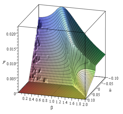
Figures 1–3 show a numerical evaluation of $\mathcal{F}(\Omega)$, expressing $\Omega$ in terms of the dimensionless parameter $h$. The scale of the $\mathcal{F}$-axis is in units of $M_{\star}$. The plots use the $n=0$ term in in (7). For $h>0$ the $n=0$ term is the full contribution. For $h<0$ the $n=0$ term is a lower bound that becomes sharp as $h\to 0_{-}$. The dramatic increase in the transition rate as $\beta$ increases past $\beta_{c}$ is apparent in all the plots.

Discussion. — We have shown that an inertial UDW detector coupled to a scalar field with a dispersion relation that violates Lorentz invariance at high energies, in a certain controlled way, exhibits drastic Lorentz violation at arbitrarily low energies. This violation occurs whenever the detector’s velocity in the distinguished frame exceeds a certain critical rapidity $\beta_{c}$, which is independent of the Lorentz violating energy scale $M_{\star}$.

The class of theories in which this phenomenon occurs includes a scalar field quantized in the polymer framework that imports techniques from loop quantum gravity. For the polymer quantized scalar field we find $\beta_{c}\approx 1.3675$, independently of the polymer mass scale.

The signature of the Lorentz violation is a sudden increase in the rate of spontaneous de-excitations and a sudden emergence of spontaneous excitations in the detector. Our linear perturbation theory analysis predicts for these transition rates a magnitude comparable to the Lorentz-breaking energy scale $M_{\star}$.

As we have assumed the interaction to last much longer than $1/M_{\star}$, and since transition probabilities can by definition not be larger than unity, the predicted value for the transition rate should not be taken literally: what the perturbative result means is that the transition probabilities grow quickly to order unity, after which a quantitative analysis would need to incorporate the back-reaction of the detector on the state of the quantum field [19, 29]. Qualitatively, however, we view the linear perturbation theory result as a reliable indicator of a violent burst of excitations and de-excitations when the detector’s rapidity exceeds $\beta_{c}$.

Since the onset of excitations and the increase in the de-excitations occur when the detector’s velocity exceeds the group velocity of high frequency waves, the phenomenon can be compared to the the Cerenkov effect. The surprise is that the effect shows up already at arbitrary small values of the detector’s energy gap, much below the energies at which the field’s group velocity is less than the speed of light.

While it may seem paradoxical that a symmetry violation at high energies can induce large low energy effects, we emphasize that instances of this kind are known to occur in quantum field theory [2, 3, 4].

The close similarity between an UDW detector and the dipole moment interaction by which an atom couples to the quantized electromagnetic field [16, 17] suggests that our prediction should apply to atoms or ions moving with a relativistic velocity, including the ions accelerated to rapidity $\beta\approx 3$ at the RHIC. The absence of observed Lorentz violations at the RHIC therefore provides a strong constraint on the possible families of modified dispersion relations.

Finally, although we have considered only an inertial detector, we anticipate that a uniformly linearly accelerated detector will exhibit a similar drastic Lorentz violation after operating so long that its rapidity in the preferred frame exceeds $\beta_{c}$. It is therefore curious that the Hawking effect appears to be robust to high energy modifications of the dispersion relation [30], but the response of a uniformly accelerated UDW detector, which in some ways is its equivalence principle dual, is not so immune.

References

- [1] G. Amelino-Camelia, Living Rev. Rel. 16, 5 (2013), eprint 0806.0339.
- [2] J. Polchinski, Class. Quant. Grav. 29, 088001 (2012), eprint 1106.6346.
- [3] J. Collins, A. Perez, D. Sudarsky, L. Urrutia, and H. Vucetich, Phys. Rev. Lett. 93, 191301 (2004), eprint gr-qc/0403053.
- [4] S. Bachmann and A. Kempf, J. Phys. A: Math. Theor. 41, 164021 (2008).
- [5] W. G. Unruh, Phys. Rev. D 14, 870 (1976).
- [6] B. S. DeWitt, in General Relativity; an Einstein Centenary Survey, edited by S. W. Hawking and W. Israel (Cambridge University Press, Cambridge, 1980).
- [7] A. Ashtekar, S. Fairhurst, and J. L. Willis, Class. Quant. Grav. 20, 1031 (2003a), eprint gr-qc/0207106.
- [8] A. Ashtekar, J. Lewandowski, and H. Sahlmann, Class. Quant. Grav. 20, L11 (2003b), eprint gr-qc/0211012.
- [9] V. Husain and A. Kreienbuehl, Phys. Rev. D 81, 084043 (2010), eprint 1002.0138.
- [10] G. M. Hossain, V. Husain, and S. S. Seahra, Phys. Rev. D 82, 124032 (2010a), eprint 1007.5500.
- [11] G. M. Hossain, V. Husain, and S. S. Seahra, Phys. Rev. D 81, 024005 (2010b), eprint 0906.2798.
- [12] S. S. Seahra, I. A. Brown, G. M. Hossain, and V. Husain, JCAP 1210, 041 (2012), eprint 1207.6714.
- [13] C. Rovelli, Quantum Gravity (Cambridge University Press, Cambridge, 2007).
- [14] T. Thiemann, Modern Canonical Quantum General Relativity (Cambridge University Press, Cambridge, 2008).
- [15] Website www.bnl.gov/rhic/complex.asp, visited August 2015.
- [16] E. Martín-Martínez, M. Montero, and M. del Rey, Phys. Rev. D 87, 064038 (2013), eprint 1207.3248.
- [17] A. M. Alhambra, A. Kempf, and E. Martín-Martínez, Phys. Rev. A 89, 033835 (2014), eprint 1311.7619.
- [18] L. C. B. Crispino, A. Higuchi, and G. E. A. Matsas, Rev. Mod. Phys. 80, 787 (2008).
- [19] B. L. Hu, S.-Y. Lin, and J. Louko, Class. Quant. Grav. 29, 224005 (2012), eprint 1205.1328.
- [20] E. Martín-Martínez and N. C. Menicucci, Class. Quant. Grav. 31, 214001 (2014), eprint 1408.3420.
- [21] A. Satz, Class. Quant. Grav. 24, 1719 (2007), eprint gr-qc/0611067.
- [22] J. Louko and A. Satz, Class. Quant. Grav. 25, 055012 (2008), eprint 0710.5671.
- [23] N. D. Birrell and P. C. W. Davies, Quantum Fields in Curved Space (Cambridge University Press, Cambridge, 1984).
- [24] M. Bojowald, Phys. Rev. Lett. 86, 5227 (2001), eprint gr-qc/0102069.
- [25] A. Ashtekar, T. Pawlowski, and P. Singh, Phys. Rev. Lett. 96, 141301 (2006), eprint gr-qc/0602086.
- [26] M. Bojowald, Living Rev. Rel. 11, 4 (2008).
- [27] A. Ashtekar and A. Barrau, Class. Quant. Grav. 32, 234001 (2015), eprint 1504.07559.
- [28] N. Kajuri (2015), eprint 1508.00659.
- [29] S. De Bièvre and M. Merkli, Class. Quant. Grav. 23, 6525 (2006), eprint math-ph/0604023.
- [30] W. G. Unruh, Phys. Rev. D 51, 2827 (1995).