Qubit quantum-dot sensors: Noise cancellation by coherent backaction,
initial slips, and elliptical precession

M. Hell^(1,2) Affiliation: (1) Peter Grünberg Institut, Forschungszentrum Jülich, 52425 Jülich, Germany
(2) JARA- Fundamentals of Future Information Technology
(3) Institute for Theory of Statistical Physics, RWTH Aachen, 52056 Aachen, Germany
(4) Institute for Quantum Information, RWTH Aachen, 52056 Aachen, Germany M. R. Wegewijs^(1,2,3) Affiliation: (1) Peter Grünberg Institut, Forschungszentrum Jülich, 52425 Jülich, Germany
(2) JARA- Fundamentals of Future Information Technology
(3) Institute for Theory of Statistical Physics, RWTH Aachen, 52056 Aachen, Germany
(4) Institute for Quantum Information, RWTH Aachen, 52056 Aachen, Germany D. P. DiVincenzo^(1,2,4) Affiliation: (1) Peter Grünberg Institut, Forschungszentrum Jülich, 52425 Jülich, Germany
(2) JARA- Fundamentals of Future Information Technology
(3) Institute for Theory of Statistical Physics, RWTH Aachen, 52056 Aachen, Germany
(4) Institute for Quantum Information, RWTH Aachen, 52056 Aachen, Germany

August 11, 2026

Abstract

We theoretically investigate the backaction of a sensor quantum dot with strong local Coulomb repulsion on the transient dynamics of a qubit that is probed capacitively. We show that the measurement backaction induced by the noise of electron cotunneling through the sensor is surprisingly mitigated by the recently identified coherent backaction [M. Hell, M. R. Wegewijs, and D. P. DiVincenzo, Phys. Rev. B 89, 195405 (2014)] arising from quantum fluctuations. This indicates that a sensor with quantized states may be switched off better than naively expected. This renormalization effect is missing in semiclassical stochastic fluctuator models and typically also in Born-Markov approaches, which try to avoid the calculation of the nonstationary, nonequilibrium state of the qubit plus sensor. Technically, we integrate out the current-carrying electrodes to obtain kinetic equations for the joint, nonequilibrium detector-qubit dynamics. We show that the sensor current response, level renormalization, cotunneling broadening, and leading non-Markovian corrections always appear together and cannot be turned off individually in an experiment or ignored theoretically. We analyze the backaction on the reduced qubit state – capturing the full non-Markovian effects imposed by the sensor quantum dot on the qubit – by applying a Liouville-space decomposition into quasistationary and rapidly decaying modes. Importantly, the sensor cannot be eliminated completely even in the simplest high-temperature, weak-measurement limit since the qubit state experiences an initial slip depending on the initial preparation of qubit plus sensor quantum dot. The slip persists over many qubit cycles, i.e., also on the time scale of the qubit decoherence induced by the backaction. A quantum-dot sensor can thus not be modeled as usual as a “black box” without accounting for its dynamical variables; it is part of the quantum circuit. We furthermore find that the Bloch vector relaxes (rate $1/T_{1}$ ) along an axis that is not orthogonal to the plane in which the Bloch vector dephases (rate $1/T_{2}$ ), blurring the notions of relaxation and dephasing times. Moreover, the precessional motion of the Bloch vector is distorted into an ellipse in the tilted dephasing plane.

pacs

73.63.Kv, 73.63.-b, 03.65.Yz

I Introduction

The ongoing effort to mitigate the qubit decoherence due to environmental noise detrimental to quantum computing has made substantial progress by identifying well-isolated two-level systems Cirac and Zoller 1995; Tyryshkin et al. 2003; Petta et al. 2005; Koch et al. 2007 and developing efficient decoupling techniques Bluhm et al. 2010; Bylander et al. 2011; Rong et al. 2011. However, active readout elements must be integrated into any quantum computer and “noise” from such sensors may soon become a relevant source of errors. Therefore, the unavoidable disturbance of the qubit evolution during a readout process gains importance, both for single-shot qubit readout Hanson et al. 2005; Barthel et al. 2010 as well as continuous qubit monitoring Il’ichev et al. 2003. Another question of central importance for qubit manipulations is which parameters should be varied to switch off a sensor most effectively when no measurement is intended to be made.

In a single-shot measurement, the goal is to achieve a strong, projective measurement that dephases the qubit state as quickly as possible. However, any measurement still takes a finite time and relaxation processes Barthel et al. 2010, excitation processes Onac et al. 2006, and incoherent detector dynamics limit the detector efficiency Korotkov and Averin 2001; Gurvitz and Berman 2005; Clerk and Stone 2004; Korotkov 2008. For continuously monitoring the qubit evolution, by contrast, one has to realize a weak measurement. The aim is here to disturb the qubit evolution as weakly as possible to retain the (partial) purity of the quantum state Oxtoby et al. 2006, while avoiding quantum jumps and the quantum Zeno effect Goan and Milburn 2001. Understanding the backaction of a weak measurement is therefore of great interest.

In this paper, we focus on the noninvasive, weak-measurement backaction exerted on a qubit by a capacitively coupled sensor quantum dot (SQD) Schoelkopf et al. 1998; Barthel et al. 2010. SQDs are attractive qubit detectors due to their strong tunability and higher signal-to-noise ratio as compared to quantum point contacts Elzerman et al. 2004; Reilly et al. 2007 and dispersive readout schemes Colless et al. 2013. This derives from the fact that an SQD is an interacting quantum system. For smaller quantum dots (QDs) than typically used for readout, the electrons may even occupy discrete energy levels. The required readout current easily leads to a strong nonequilibrium and nonstationary sensor state. This altogether makes the description of the backaction arising from an SQD on a qubit challenging. Thus, typical weak-coupling approaches to decoherence assuming an environment in equilibrium with a continuous spectrum Paladino et al. 2002; Grishin et al. 2005; Bergli et al. 2009; Shnirman et al. 2005; Ithier et al. 2005; Chirollli and Burkard 2008; Galperin et al. 2004 cannot be applied here and naive extensions are prone to errors as we will illustrate. Understanding the intertwined evolution of SQD and qubit is of key importance to understand the measurement backaction Shnirman and Schön 1998; Makhlin et al. 2001; Gurvitz and Berman 2005; Gurvitz and Mozyrsky 2008; Hell et al. 2014.

Out of these challenges arises the question which physical effects have to be included for a consistent description of the measurement backaction of a sensor QD on a qubit. For the qubit, we consider the simplest model that involves capacitive readout, a charge qubit, realized as a double quantum dot. An important aspect lies in the type of setup considered, namely that of indirect detection: one measures the conductance of a sensor QD in the attached electrodes, while only the SQD capacitively interacts with the qubit, see Fig. 1. To maximize the sensitivity, the SQD is operated at the threshold to the Coulomb blockade regime. Here, the conductance of the SQD shows the strongest response to small qubit-induced level shifts. Previous studies addressing the backaction of an SQD on a qubit in this regime focused mainly on the lowest-order approximation in the tunnel coupling $\Gamma$ of the SQD to the attached electrodes Shnirman and Schön 1998; Makhlin et al. 2000; Makhlin et al. 2001; Gurvitz and Berman 2005; Gurvitz and Mozyrsky 2008; Oxtoby et al. 2006, strictly valid when operated in the single-electron tunneling (SET) regime. There are two main reasons for going beyond this approximation.

The first reason relates to the backaction on the qubit and its dependence on the level position, experimentally controlled by gate voltages. This is important since the level position is one of the key experimental control parameters by which one can try to switch off the sensor backaction. In this approximation, the leading-order rates (SET $\propto\Gamma$ ) become exponentially small when the level position ( $\varepsilon$ ) of the SQD is tuned away from the electrochemical potentials of the electrodes $(\mu_{r})$ . Thus, when one is interested in the backaction at the onset of Coulomb blockade, next-to-leading order $\propto\Gamma^{2}$ cotunneling processes should also be accounted for because they are only algebraically suppressed, scaling as $1/(\varepsilon-\mu_{r})$ . One would thus naively expect that the backaction is suppressed only inversely proportional to the detuning from resonance. Yet, level-renormalization effects should also be considered; they lead to level shifts that depend logarithmically on the level position $\varepsilon$ and therefore the response of the level renormalization to the measurement perturbation also scales as $1/(\varepsilon-\mu_{r})$ . A central finding of our study is that level-renormalization effects in fact mitigate the naively expected cotunneling decoherence.

A second reason for going beyond the lowest-order approximation comes in view when one takes into account the experimentally used sensor signal: if one accounts for the first nonvanishing contributions $\propto\lambda\Gamma/T$ that produce a nonzero sensor signal, one has to include also renormalization effects since they appear in the same order. Basically, if one has time to measure, one has time to fluctuate as well. As already emphasized in Ref. Hell et al. 2014, incorporating terms $\propto\lambda\Gamma/T$ is another reason that forces us to keep also cotunneling processes $\propto\Gamma^{2}/T$ since in the weak-measurement limit $\lambda\ll\Gamma$ the latter are larger. Only when one is not interested in the sensor current, one can consistently neglect cotunneling and renormalization effects by taking the high-temperature limit: as we show, they must either be kept or neglected together.

The above-mentioned processes combine in a nontrivial way to give three types of backaction on the qubit Hell et al. 2014. First, both SET and cotunneling processes contribute to a stochastic switching of the SQD charge state. This switching generates a randomly fluctuating effective magnetic field acting on the qubit Bloch or isospin vector Ithier et al. 2005; Chirollli and Burkard 2008. This “noise” – called here the stochastic backaction – leads to a shrinking of the Bloch vector, i.e., to decoherence. In addition, there is a dissipative backaction, which is the flip-side of the measurement action: it arises whenever one accounts for a nonzero response of the sensor SET tunnel rates to the qubit state and therefore a nonzero sensor signal. Finally, there is a coherent backaction, the most striking finding of Ref. Hell et al. 2014. It arises from the above-mentioned level-renormalization response and translates into torque terms involving the qubit Bloch vector. These torques and related precession effects are similar to those emerging in various other QD transport setups: It is well-known that tunneling processes can produce exchange fields leading to an (iso)spin precession in the context of spintronics J. König and J. Martinek 2003; Braun et al. 2004, double dots Wunsch et al. 2005, molecular quantum dots Donarini et al. 2006; Schultz 2010, and superconducting devices Governale et al. 2008. All these level-renormalization effects arise from quantum fluctuations of electrons by tunneling into the attached electrodes. In this respect, a qubit coupled to a sensor QD is not different.

An interesting question is how these different types of backaction relate to the information gained during the measurement process. Clearly, the quasistationary time-dependent current through the sensor contains information about the qubit state and at the same time causes decoherence of the qubit. However, besides this fundamentally unavoidable backaction, the decoherence induced by the detector can be stronger. This can be formulated in terms of general inequalities relating the noise of the measured operator (here the position of the qubit electron) to the noise of the measurement signal (here the current) and additional noise cross terms Clerk et al. 2010. The situation considered in this paper is far away from the quantum limit (meaning the above-mentioned inequality is far from being satisfied with equality).
A part of our work actually focuses on a simple limit when only the stochastic backaction is accounted for but dissipative and coherent backaction are neglected. The SQD then acts rather as an “ordinary” environment and no information is obtained during the operation – a situation relevant when the detector is supposed to be switched off. Yet, even in this simple limit, there are effects beyond the scope of the picture developed in Ref. Clerk et al. 2010: the fast relaxation due to switching on the sensor may affect the qubit state also in a way that depends on the initial dynamical variables of the sensor. This is not captured at all by the noise inequalities mentioned above. The explicit time evolution of the sensor, which is not considered in Ref. Clerk et al. 2010, is thus also crucial to understand the backaction on the qubit. An interesting question arising from this insight is how this backaction effect has to be assessed in view of the information gain. Our work could thus spur new activity on the topic of information gain during the measurement.
The impact of the three backaction effects on the full transient dynamics of the qubit so far remained an outstanding question that we address in this article (the analysis in Ref. Hell et al. 2014 was restricted to the stationary state). Our analysis is divided into two parts.
Part 1. The main point of this paper is to eliminate the electrodes’ degrees of freedom Makhlin et al. 2000 and to analyze the transient dynamics within the resulting physical picture of the coupled SQD-qubit dynamics. In this way, we can deal with the nontrivial interplay of the SQD-qubit coherence, strong local Coulomb interaction in the SQD, nonequilibrium conditions imposed by the attached electrodes, as well as both leading (SET) and next-to-leading order effects in the tunneling (cotunneling). The necessary inclusion of the latter furthermore forces us to extend Ref. Hell et al. 2014 by including also the leading memory effects on the sensor-qubit system due to the tunneling to the electrodes, which is necessary for the study of the transient qubit dynamics. (For the stationary state, which we studied in Ref. Hell et al. 2014, they can be be ignored without making additional approximations.) The importance of memory effects for the dynamics when going beyond weak coupling is known especially since Ref. Braggio et al. 2006, see also Refs. Splettstoesser et al. 2006; Flindt et al. 2008; Flindt et al. 2010; Braggio et al. 2009; Splettstoesser et al. 2010; Goorden et al. 2004 and progress for strong backaction Hartmann and Wilhelm 2007; Kennes et al. 2013. Non-Markovian corrections have also been studied in related contexts, such as the backaction of a quantum point contact on a double dot Hartmann and Wilhelm 2007; Braggio et al. 2009 or quantum-feedback control based on quantum measurements Rebentrost et al. 2009; Floether et al. 2012. The various effects of non-Markovian processes remain, however, an uncharted territory Glaser et al. 2015.
The central result in our case are the kinetic equations (III.2.2) for the system of qubit plus quantum-dot sensor. The equations reveal the above three-fold nature of the backaction of the sensor QD on the qubit; importantly, the relevant energy scale for this backaction is not simply the internal capacitive interaction $\lambda$ (SET-induced stochastic backaction) but additionally involves the energy scale $\Gamma\lambda/T$ (dissipative and coherent backaction involving transport processes).

Our kinetic equation furthermore allows us to identify slowly evolving quasistationary modes – containing the qubit evolution – and faster evolving decay modes reflecting the dissipative SQD dynamics due to its coupling to the electrodes. The coupling between these modes generates the total backaction on the qubit and is mediated by all three types of backaction. To account for all these backaction effects, it is indispensable to keep the capacitive interaction ( $\lambda\neq 0$ ) when integrating out the electrodes. In this aspect, our work differs from the otherwise closely related approach of Ref. Emary 2008, which starts out from the assumption that the electrodes affect exclusively the SQD. There, all backaction effects derive only from the internal interaction, i.e., the stochastic backaction.

A surprising finding of our analysis is that the total backaction exhibits a strong reduction when tuning the SQD towards the Coulomb blockade regime: we find that the coherent backaction actually cancels the cotunneling (“broadening”) corrections in the coupling of the quasistationary to the decay modes. This eliminates the naively expected leading power-law dependence $\propto 1/(\varepsilon-\mu_{r})$ of the backaction, affecting also the decoherence time scales. This indicates that a sensor with quantized orbital states can be switched off more efficiently by controlling its gate voltage than naively expected, the first important experimental implication of this article. This requires, however, to prepare the sensor state in a controlled way to avoid a slip of the qubit state (see part 2 below).

It is important to emphasize already here that the coherent backaction, which is responsible for this mitigation, is not an independent mechanism that can be “added” to counteract cotunneling noise. Instead, it arises together with cotunneling as an integral part of quantum fluctuation effects of the qubit-sensor system when consistently describing all types of backaction. Notably, we show that this mitigation is not captured by widely-used classical stochastic fluctuator models and can also be easily overlooked in Born-Markov approaches that integrate out the entire environment of the qubit (i.e., including the SQD). The effect of the exchange of electrons between the SQD and the electrodes can thus not be fully captured by classical switching of the SQD charge state. We also review and compare in detail our results with earlier works and pinpoint a number of limitations of standard approaches.

The prominent role of renormalization effects underlying the coherent backaction distinguishes a QD sensor with few, discrete energy levels from what can be expected for a sensor with a continuous energy spectrum. The recent study Lindebaum and König 2011 showed that similar torque terms appearing in a spintronic context are much suppressed in single-electron transistors (continuous spectrum) as opposed to QDs (discrete spectrum). In the former case, renormalization effects tend to nullify when averaging over their continuous energy spectrum. This motivates the extensive analysis of the detection of a qubit state by a sensor QD undertaken in this paper. Our work raises the interesting question to which extent backaction effects due to renormalization effects are suppressed in a single-electron transistor.

Part 2. One might think that following the above description one can in a second step eliminate the sensor QD from the description to obtain an effective theory for the qubit only. However, already on general grounds, this is questionable: specific to our indirect detection problem is that the environment of the qubit is not stationary. Moreover, initial correlations between SQD and qubit – both microscopic systems – might exist. When integrating out the environment, the factorizability and the stationarity of the environment are, however, often invoked to eliminate the so-called slip of the initial condition for the subsystem Gaspard and Nagaoka 1999 coming from the initial state of the environment and its short-time transient evolution. To illustrate this point, we analyze in more detail the simpler high-temperature limit where the complications due to cotunneling and coherent backaction can be consistently ignored. Even in this high-temperature, weak-measurement limit the qubit develops a slip of order $\lambda/\Gamma$ on a time scale $t<1/\Gamma$ , which is beyond the control over the qubit system alone. The slip depends explicitly on the initial qubit-sensor state. The second experimental implication of our work is that the dynamical state of the sensor and its correlations with the qubit cannot be ignored and must be brought under experimental control. This slip effect is cumulative, e.g., it results in phase shifts that still affect the qubit on much longer time scales $t\sim 1/\lambda\gg 1/\Gamma$ relevant to the readout. By contrast, the relevant time scales $T_{1}$ (relaxation) and $T_{2}$ (dephasing) of the transient qubit dynamics for times $t\gg 1/\Gamma$ do not depend on the initial sensor QD state.
The precession axis of the qubit Bloch vector also turns out to be independent of the initial state. In the simple high-temperature limit, we furthermore identify an additional effect of the (purely stochastic) backaction, which is to induce a tilt of the Bloch vector precession axis. We find that the circular isospin precession becomes slightly elliptical in the presence of the detector, adding as a fingerprint oscillations to the exponential decay of the qubit-state purity. This mixes the notions of relaxation and dephasing as we will see. It is an interesting question how these effects behave at low temperature and strong qubit-sensor coupling where they have received little attention so far.

Outline. After this topical outline, we now present the organization of the sections of the paper and the key equations. In Sec. II, we briefly review the generic indirect readout model of Ref. Hell et al. 2014 and discuss the dynamical variables that are needed to describe the mixed quantum state of the joint qubit-sensor system. This requires two isospins, which capture both the reduced qubit state as well as the correlations with the sensor QD.
After this, we outline the key technical challenges of our approach in Sec. III, deferring details to the App. A, and we present the time-local kinetic equation (III.2.2) for the coupled sensor QD plus qubit system. In App. A, we further discuss the importance of including non-Markovian corrections to retain the positivity of the reduced density operator. Without further approximations, we identify the relevant unperturbed modes ( $\lambda=0$ ) with the electrodes integrated out. From the representation of the kinetic equation () in these modes we prove the exact cancellation between the coherent backaction and the cotunneling (“broadening”) noise [Eq. (137)]. We furthermore study the implications for the dependence of the total backaction on various experimentally relevant parameters (tunneling-rate asymmetries, bias, and gate voltages). From the formal solution of the effective quasistationary mode evolution [Eqs. (148) and (149)], with details given in Appendix B, we infer that the qubit evolution is non-Markovian and exhibits a slip of the initial condition that we characterize in Appendix C. Initial slips generally go hand in hand with non-Markovian dynamics as Refs. Haake and Lewenstein 1983; Geigenmüller et al. 1983; Haake and Reibold 1985; Gaspard and Nagaoka 1999; Flindt et al. 2008; Wilhelm 2008 and the references therein point out. Initial entanglement between a qubit and its environment, one cause of initial slips, can drastically affect the qubit coherence Wilhelm 2008.
In Sec. IV, we attempt to integrate out the sensor QD to derive an effective Liouvillian [Eq. (165)] that effectively incorporates its fast switching dynamics. We then focus on the analytically tractable case of high temperature. This suffices to illustrate the general importance of initial slips in the context of detector backaction [Eq. (166)], the breakdown of orthogonality of relaxation and dephasing qubit modes, and the exponentially damped oscillatory but elliptical precession of the qubit Bloch vector. In this high-temperature limit, we obtain tangible expressions for the qubit relaxation and dephasing rates, expanded to leading order in $\lambda/\Gamma$ . In Sec. V, we compare our results with semiclassical stochastic fluctuator models as well as Born-Markov and exact quantum approaches to provide further insight into the origin of the coherent backaction. In the accompanying Appendix D we show how the coherent backaction affects the qubit phase evolution in a way that is not accounted for by semiclassical stochastic fluctuator approaches. We summarize our findings in Sec. VI.

Refer to caption — Figure 1: Sensor quantum dot (SQD) tunnel-coupled to source and drain electrodes and capacitively coupled to a qubit, whose different logical states involve two possible positions, left and right, in a double quantum dot. If the qubit electron is left (a) or right (b), the Coulomb repulsion to the SQD electron is larger or smaller, respectively, compared to the full delocalization of the qubit electron.

II Indirect detection

II.1 Model

We analyze the indirect detection setup sketched in Fig. 1: the readout ( $H_{I}$ ) of a double-quantum dot charge qubit ( $H_{Q}$ ) by a proximal sensor quantum dot ( $H_{S}$ ), which in turn is read out ( $H_{T}$ ) by the conductance of the transport current in one of the attached electrode reservoirs ( $H_{R}$ ). The model we use, discussed in detail in Ref. Hell et al. 2014, thus consists of three “layers” with their respective interactions:

\displaystyle H

\displaystyle=

\displaystyle H_{Q}+(H_{I}+H_{S})+(H_{T}+H_{R}).

(1)

This models the essential physics found in many experiments on QD qubits and can be extended to superconducting qubits Devoret and Martinis 2005 as well as to spin qubits if measured by spin-to-charge conversion Elzerman et al. 2004; Barthel et al. 2010.

Qubit. The qubit is realized as a charge qubit, a single electron occupying a double quantum dot. This electron can reside either on the left dot, denoted by the state ${\color[rgb]{0,0,0}|}L{\color[rgb]{0,0,0}\rangle}$ , or on the right dot, denoted by the state ${\color[rgb]{0,0,0}|}R{\color[rgb]{0,0,0}\rangle}$ . The qubit state is represented by the ensemble average ${\color[rgb]{0,0,0}{\bm{\tau}}}={\color[rgb]{0,0,0}\langle}\hat{{\color[rgb]{0,0,0}{\bm{\tau}}}}{\color[rgb]{0,0,0}\rangle}$ of an operator $\hat{{\color[rgb]{0,0,0}{\bm{\tau}}}}$ (corresponding to an isospin $\hat{{\color[rgb]{0,0,0}{\bm{\tau}}}}/2$ ) with components

\displaystyle\hat{\tau}_{i}

\displaystyle=

\displaystyle\sum_{l,l^{\prime}=L,R}(\sigma_{i})_{ll^{\prime}}{\color[rgb]{0,0,0}|}l{\color[rgb]{0,0,0}\rangle}{\color[rgb]{0,0,0}\langle}l^{\prime}{\color[rgb]{0,0,0}|}.

(2)

Here, $\sigma_{i}$ denotes the Pauli matrix for $i=x,y,z$ . The average $z$ component $\tau_{z}$ quantifies the imbalance between the probabilities for finding the qubit electron in the left orbital rather than in the right orbital, while $\tau_{x}$ and $\tau_{y}$ quantify coherences between the left and right occupation. The general form of the Hamiltonian of the isolated qubit is

\begin{array}[]{lll}H_{Q}&=&{\bm{\Omega}}\cdot\hat{{\bm{\tau}}}\text{/}2,\end{array}

(3)

in which the qubit field ${\bm{\Omega}}$ is used in applications to control the qubit evolution: it induces coherent tunneling of the qubit electron between the two dots ( $\Omega_{x}$ , $\Omega_{y}$ ) combined with a detuning ( $\Omega_{z}$ ). In our analysis, ${\bm{\Omega}}$ is constant in time and later on, when we discuss tangible results, we will chose ${\bm{\Omega}}=\Omega\mathbf{e}_{x}$ . However, unless stated otherwise, we first keep ${\bm{\Omega}}$ general.

Sensor quantum dot. The sensor quantum dot (SQD or sensor QD) is modeled as a single, interacting, spin-degenerate orbital level with Hamiltonian $H_{S}=\varepsilon\hat{n}+U\hat{n}_{\uparrow}\hat{n}_{\downarrow}$ . Here, $\hat{n}_{\sigma}=d^{{\dagger}}_{\sigma}d_{\sigma}$ is the number operator for electrons with spin $\sigma=\uparrow,\downarrow$ , where $d_{\sigma}$ denotes the corresponding field operator, and $\hat{n}=\hat{n}_{\uparrow}+\hat{n}_{\downarrow}$ is the total electron number operator. We take the Coulomb repulsion energy $U$ here to be the largest energy scale (except for the bandwidth $2W$ of the electrodes), in accordance with typical experimental situations. We therefore exclude the double occupation of the sensor QD orbital in the following. This allows us to reduce the model to

\begin{array}[]{lllllll}H_{S}&=&\varepsilon\hat{P}^{1},&&\hat{P}^{1}&=&\sum_{\sigma}{\color[rgb]{0,0,0}|}\sigma{\color[rgb]{0,0,0}\rangle}{\color[rgb]{0,0,0}\langle}\sigma{\color[rgb]{0,0,0}|},\end{array}

(4)

if we accordingly adjust the high-energy cutoffs in the electrodes [discussed below Eq. (49)]. In the considered subspace, we can replace $\hat{n}=\hat{P}^{1}$ . For the readout one tunes the level position $\varepsilon=-V_{g}$ by a gate voltage $V_{g}$ close to the electrochemical potentials of one of the electrodes. While the spin of the qubit electron is irrelevant (it was not written above since the readout couples to the charge, see below), it is important to include the spin degree of freedom of the SQD because the spin degeneracy enters into the tunneling rates.

Electrodes. The final stage of the readout involves the electrodes, treated as noninteracting reservoirs of electrons with spin:

\begin{array}[]{lll}H_{R}&=&\sum_{r,k,\sigma}\omega_{rk\sigma}c^{{\dagger}}_{rk\sigma}c_{rk\sigma},\end{array}

(5)

with the field operators $c_{rk\sigma}$ ( $c^{{\dagger}}_{rk\sigma}$ ) acting on the electrons in orbital $k$ with spin $\sigma$ in the source ( $r=s$ ) and the drain ( $r=d$ ), respectively. These are each held in equilibrium with a common temperature $T$ , but at different electrochemical potentials $\mu_{s}=V_{b}\text{/}2$ and $\mu_{d}=-V_{b}/2$ by a applying a bias voltage $V_{b}$ .

Readout. The indirect readout of the qubit state using the sensor QD involves two couplings: the first one is the capacitive interaction of the SQD electron charge $\hat{n}$ with the charge polarization $\hat{\tau}_{z}$ of the qubit:

\begin{array}[]{lll}H_{I}&=&\hat{n}{\bm{\lambda}}\cdot\hat{{\bm{\tau}}}\text{/}2.\end{array}

(6)

The measurement vector ${\bm{\lambda}}$ specifies both the basis in which one measures and the measurement strength $\lambda$ :

\begin{array}[]{lll}{\bm{\lambda}}&=&\lambda\mathbf{e}_{z}.\end{array}

(7)

Thus, depending on the qubit state, the sensor QD level experiences an energy/gate-voltage offset of at most $\pm\lambda/2$ [see Figs. 1 (a) and 1(b)]. This in turn affects the conductance measured in one of the electrodes due to tunneling to and from the SQD:

\begin{array}[]{lll}H_{T}&=&\sum_{r,k,\sigma}t_{r}d^{{\dagger}}_{\sigma}c_{rk\sigma}+\text{H.c.}\end{array}

(8)

The strength of this second coupling involved in the readout is quantified by the tunnel rates $\Gamma_{r}=2\pi|t_{r}|^{2}\nu_{r}$ , where we take both the tunneling amplitude $t_{r}$ and the density of states $\nu_{r}$ to be spin $(\sigma)$ - and energy $(k)$ -independent within the electrode bandwidth $2W$ .

The threefold layered structure of this indirect detection (negligible direct coupling of the electrodes to the qubit) is reflected in our theoretical analysis of the measurement backaction. In Sec. III.3, we first eliminate the ‘‘outer’’ detection layer -- the electrodes -- in favor of effective equations describing the joint SQD-qubit dynamics ¹¹ 1 The first step of our approach is in principle generally possible at least for weak tunnel coupling $\Gamma$ , i.e., not limited to the weak-measurement situation we study in this paper.. In Sec. IV, we then attempt to integrate out the “inner” detection layer – the SQD – to find the effective qubit evolution.

II.2 Weak-measurement and weak-tunneling limit

We consider a sensor with a fast response, i.e., the internal dynamics of qubit plus sensor QD is slow as compared to the electron tunneling dynamics induced by the attached electrodes:

\displaystyle\Delta

\displaystyle\sim

\displaystyle\lambda,\Omega\ \ \ll\ \ \Gamma.

(9)

This condition means physically that many electrons pass through the SQD during its interaction time with the qubit ( $\lambda\ll\Gamma$ ) — a weak measurement is performed. Moreover, if ${\bm{\Omega}}$ lies in the $x$ - $y$ plane, the internal qubit evolution describes a coherent tunneling of the qubit electron with dwell times of electrons in the SQD that are much smaller than the period of a qubit cycle $(\Omega\ll\Gamma)$ . Each electron sees a “snapshot” of the SQD-plus-qubit state. If we assumed $\Gamma\lesssim\Omega$ instead (but still weak measurement $\lambda\ll\Gamma$ ), the readout would be too slow to resolve any qubit evolution.

As we see below in Sec. III, the leading-order response of the tunnel rates to a measurement-induced gate voltage offset $\sim\lambda$ is given by $\Gamma\lambda/T$ . This, in return, induces a dissipative backaction affecting the polarization of the qubit that also scales as $\Gamma\lambda/T$ . Moreover, when condition (9) holds, the tunneling also affects the isospin coherences of the qubit-SQD state. This is well-known from the analysis of two-level systems coupled to a reservoir: Here, the density-operator coherences in the energy basis matter when the levels (here split by $\Delta$ ) are degenerate on the scale of the coupling (here $\Gamma$ ) to the environment. In our case, the two levels correspond to the sensor QD and the qubit, each being a two-state system. One has to carefully identify which coherences are relevant, which is done below in Sec. II.3. These coherences are affected by tunneling processes: The simple physical intuition behind this is that if an electron on the sensor has time to interact with the qubit and change the current, it certainly has time to fluctuate into the electrodes. This leads to a response of the level renormalization and results in a coherent backaction which scales as $\Gamma\lambda/T$ , i.e., in the same way as the response of the sensor tunneling rates resulting in the dissipative backaction. This is a central result of Ref. Hell et al. 2014 and here we explore its effect on transient dynamics.

It should thus be noted that the energy scale for backaction on the qubit is not simply $\lambda$ (from the internal interaction $H_{I}$ ) but also $\lambda\Gamma/T$ , the scale of effective dissipative and coherent coupling between sensor QD and qubit, which are induced by tunneling processes. In a way, these couplings account for an indirect interaction of the qubit with the electrodes extending the approach of Ref. Emary 2008. This is thus another relevant perturbative scale for a weak-measurement expansion, besides the scale $\lambda$ itself, see Ref. Hell et al. 2014 for a detailed exposition.

Another crucial point for this work is that if terms of order $\Gamma\lambda/T$ are taken into account and $\lambda\ll\Gamma$ , then at least cotunneling terms scaling as $\Gamma^{2}/T$ must also be accounted for (if not even higher-order tunneling terms). We can neglect higher-order tunneling processes beyond cotunneling if we restrict the temperatures such that

\displaystyle\Gamma^{2}/T

\displaystyle\ll

\displaystyle\lambda.

(10)

This condition means that the cotunneling-induced noise imposes only a weak perturbation of the qubit. Taken together, we employ here a weak-coupling limit in two ways, namely that of weak measurement and weak tunneling:

\begin{array}[]{lllll}\Gamma/T&\ll&\Delta/\Gamma&\ll&1\end{array}.

(11)

Note that by Eq. (10) this imposes a stronger condition than the usual weak-tunneling assumption $\Gamma/T\ll 1$ alone. We next discuss the dynamical variables needed to describe the measurement backaction.

II.3 Charge-specific isospins and qubit decoherence

To describe both the backaction of the sensor on the qubit as well as to compute the signal current through the sensor QD, one needs at least the reduced density operator $\rho(t)$ of the combined qubit plus SQD system obtained by tracing over the electrodes. Even though we do not analyze the sensor signal here, the signal is of course of high interest to gain insight into, e.g., the efficiency of the measurement Korotkov and Averin 2001; Gurvitz and Berman 2005; Clerk and Stone 2004; Korotkov 2008. Studying the backaction in a situation where the sensor signal current is not negligible, is an experimentally highly relevant situation, which we pursue in this paper.
The relevant part of the SQD-qubit density operator $\rho(t)$ can be expanded as follows Hell et al. 2014:

\displaystyle\rho(t)

\displaystyle=

\displaystyle\frac{1}{2}\sum_{n}\hat{P}^{n}\otimes\left[p^{n}(t)\hat{\mathbbm{1}}+\sum_{i}\tau^{n}_{i}(t)\hat{\tau}_{i}\right].

(12)

Here, $\hat{P}^{n}$ denotes the projector onto the charge states $n=0,1$ of the sensor QD. The numbers $p^{n}(t)=\operatorname{tr}(\hat{P}^{n}\rho(t))$ give the probability for the sensor QD to be in the respective charge state $n=0,1$ , which for any time $t$ sum up to one due to the probability conservation: $p^{0}+p^{1}=1$ . The only irrelevant coherences (off-diagonal matrix elements in the energy basis) of $\rho$ are those involving different charge states on the sensor. These can be shown to decouple from the relevant part due to the charge conservation by the tunneling. However, all remaining qubit-SQD density matrix elements including their coherences must be kept in (12). These are the six numbers $\tau^{n}_{i}(t)=\operatorname{tr}(\hat{P}^{n}\hat{\tau}_{i}\rho(t))$ , which are the averages of the isospin components $i=x$ , $y$ , and $z$ for the two sensor QD charge states $n=0$ or $1$ , respectively. To describe the correlated SQD-qubit system, one thus needs two charge-specific isospins ${\color[rgb]{0,0,0}{\bm{\tau}}}^{0}$ and ${\color[rgb]{0,0,0}{\bm{\tau}}}^{1}$ . Based on Eq. (12), it is convenient to introduce the following column representation of the density operator:

\displaystyle{\bm{\rho}}

\displaystyle=

\displaystyle\left(\begin{array}[]{c}p^{0}\\ p^{1}\\ {\color[rgb]{0,0,0}{\bm{\tau}}}^{0}\\ {\color[rgb]{0,0,0}{\bm{\tau}}}^{1}\end{array}\right).

In this form, one distinguishes the charge and isospin part, respectively, but the isospin part is still kept basis independent. In other words, we may represent ${\color[rgb]{0,0,0}{\bm{\tau}}}^{0}$ and ${\color[rgb]{0,0,0}{\bm{\tau}}}^{1}$ in a different orbital basis than the one used in definition (2) if we transform the directions of ${\bm{\lambda}}$ and ${\bm{\Omega}}$ accordingly.

We now further explore the physical meaning and importance of the two charge-specific isospins. By construction, they sum up to the total isospin,

\displaystyle{\color[rgb]{0,0,0}{\bm{\tau}}}

\displaystyle=

\displaystyle{\color[rgb]{0,0,0}{\bm{\tau}}}^{0}+{\color[rgb]{0,0,0}{\bm{\tau}}}^{1},

(18)

which is often of main interest. This is the usual Bloch vector that describes the state of the qubit, i.e., its reduced density operator. One can easily show that a single Bloch vector can describe the joint SQD-qubit state only if it is factorizable. In other words, if

\displaystyle\rho

\displaystyle=

\displaystyle\rho_{S}\otimes\rho_{Q}=\left(\sum_{n}p^{n}\hat{P}^{n}\right)\otimes\frac{1}{2}\left(\hat{\mathbbm{1}}+\sum_{i}\tau_{i}(t)\hat{\tau}_{i}\right),

then the charge-specific isospins are given by ${\bm{\tau}}^{0}=p^{0}{\bm{\tau}}$ and ${\bm{\tau}}^{1}=p^{1}{\bm{\tau}}$ , respectively, by comparing Eq. () with Eq. (12). The other combination of the two isospins,

\displaystyle{\bm{\delta}}:=p^{0}{\bm{\tau}}^{1}-p^{1}{\bm{\tau}}^{0},

(20)

quantifies the nonfactorizability of the qubit-sensor density operator:

\displaystyle\rho=\rho_{S}\otimes\rho_{Q}

\displaystyle\Leftrightarrow

\displaystyle{\bm{\delta}}=0.

(21)

We emphasize that the nonfactorizability is crucial to describe the readout and its backaction on the qubit state ${\color[rgb]{0,0,0}{\bm{\tau}}}$ . We will see in Sec. III.3.1 below Eq. (III.3.1) that the deviation ${\bm{\delta}}$ has no impact on the qubit evolution only if the qubit and sensor are strictly decoupled ( $\lambda=0$ ). For the coupled case ( $\lambda\neq 0$ ), which is of interest, we have to keep the individual dynamics of ${\bm{\tau}}^{0}$ and ${\bm{\tau}}^{1}$ .
The relevance of the two isospins for the decoherence can be seen explicitly from the equation of motion for $|{\color[rgb]{0,0,0}{\bm{\tau}}}(t)|^{2}$ , which characterizes the purity of the isospin state:

\displaystyle\begin{array}[]{lllll}\frac{d}{dt}[|{\color[rgb]{0,0,0}{\bm{\tau}}}|^{2}]&=&2\dot{{\bm{\tau}}}\cdot{\bm{\tau}}&=&-2{\color[rgb]{0,0,0}{\bm{\lambda}}}\cdot({\color[rgb]{0,0,0}{\bm{\tau}}}^{0}\times{\color[rgb]{0,0,0}{\bm{\tau}}}^{1}),\end{array}

where we inserted after the first equality

\displaystyle\begin{array}[]{lll}\dot{{\bm{\tau}}}&=&{\bm{\Omega}}\times{\bm{\tau}}+{\bm{\lambda}}\times{\bm{\tau}}^{1}.\end{array}

Equation (II.3) is an exact result which can be obtained from the Heisenberg equation of motion for ${\bm{\tau}}$ with respect to the full Hamiltonian (1). The only essential assumption on which Eq. (II.3) relies is the indirect readout structure of our setup, i.e., $[H_{T},H_{Q}]=0$ . It thus holds generally for any ${\bm{\Omega}}$ and any tunneling $\Gamma$ . Preservation of this exact equation imposes an exact isospin sum rule [discussed below Eq. (III.2.2)], which any kinetic equation for $\rho$ should satisfy: This was only realized recently, see Refs. Salmilehto et al. 2012 and Hell et al. 2014, in particular, see Appendices D and E.

Equation (II.3) shows that the reduction of the purity of the qubit state appears only due to noncollinearities of ${\color[rgb]{0,0,0}{\bm{\tau}}}^{0}$ and ${\color[rgb]{0,0,0}{\bm{\tau}}}^{1}$ . These noncollinearities develop because of the readout: the isospins ${\color[rgb]{0,0,0}{\bm{\tau}}}^{0}$ and ${\color[rgb]{0,0,0}{\bm{\tau}}}^{1}$ are subject to different effective “magnetic” fields depending on the charge state $n$ of the sensor QD. To see this, we rewrite $H_{Q}+H_{I}=\hat{\mathbf{B}}_{\operatorname{eff}}(\hat{n})\cdot\hat{{\bm{\tau}}}/2$ with an effective field acting on the isospin $\hat{{\color[rgb]{0,0,0}{\bm{\tau}}}}$ ,

\displaystyle\hat{\mathbf{B}}_{\operatorname{eff}}

\displaystyle=

\displaystyle\tilde{{\bm{\Omega}}}+{\bm{\lambda}}\delta\hat{n},

(26)

where $\delta\hat{n}=\hat{n}-\langle\hat{n}\rangle$ and ${\color[rgb]{0,0,0}\langle}\hat{n}{\color[rgb]{0,0,0}\rangle}=\operatorname{tr}(\hat{P}^{1}\rho)=p^{1}$ . Here, the first part is the mean field,

\displaystyle\tilde{{\bm{\Omega}}}

\displaystyle=

\displaystyle{\bm{\Omega}}+\langle\hat{n}\rangle{\bm{\lambda}},

(27)

which the isospin experiences due to the internal isospin field ${\bm{\Omega}}$ and the average field caused by the mean charge ${\color[rgb]{0,0,0}\langle}\hat{n}{\color[rgb]{0,0,0}\rangle}=p^{1}$ on the sensor QD with respect to the exact total density operator $\rho$ . The mean-field contribution $\tilde{{\bm{\Omega}}}$ to $\hat{\mathbf{B}}_{\operatorname{eff}}$ is the same for both charge-specific isospins, ${\bm{\tau}}^{0}$ and ${\bm{\tau}}^{1}$ , and therefore not responsible for the qubit-state decay. The mean SQD occupation $\langle\hat{n}\rangle=p^{1}$ merely tilts the qubit precession axis and changes its frequency contributing to the detuning of the qubit. Note that the average is here an ensemble average but not a time average since $p^{1}=p^{1}(t)$ can change in time with the state $\rho(t)$ . The qubit decay is induced by the second, fluctuating contribution ${\bm{\lambda}}\delta\hat{n}$ to Eq. (26), where $\delta\hat{n}=\hat{n}-\langle\hat{n}\rangle$ is the charge-state dependent deviation from the mean field. This generates a noncollinearity of ${\color[rgb]{0,0,0}{\bm{\tau}}}^{0}$ and ${\color[rgb]{0,0,0}{\bm{\tau}}}^{1}$ , which reduces the purity of the qubit state by Eq. (II.3).

Even though our approach does not make use of the decomposition into a mean-field and a fluctuating part, we can identify both effects in our results in Sec. III.5. We will first identify $p^{1}=p^{1}_{\operatorname{st}}$ with the state of the SQD in the stationary limit, in which the ensemble and the time average are equal. We further connect more precisely the decoherence rates to the components of the fluctuating part ${\bm{\lambda}}\delta\hat{n}$ along and perpendicular to the mean field $\tilde{{\bm{\Omega}}}$ in Sec. IV.1 (in accordance with the literature Ithier et al. 2005; Chirollli and Burkard 2008). This accounts for what we call stochastic backaction on the qubit by the sensor QD. This effect is also present for single-electron transistor sensors with a continuum of electronic levels, but (classically) quantized charge states.

However, there are also a dissipative and a coherent backaction effect Hell et al. 2014 (see Sec. II.2). As we discuss below, they modify the relative orientations of ${\color[rgb]{0,0,0}{\bm{\tau}}}^{0}$ and ${\color[rgb]{0,0,0}{\bm{\tau}}}^{1}$ and therefore affect the qubit decay as well. This mechanism — first noted in Ref. Hell et al. 2014 — derives from a renormalization effect induced by the interplay of the readout interactions ( $\lambda$ ) and the tunneling on and off the sensor QD ( $\Gamma$ ) as discussed in Sec. III. It results in isospin torques similar to those encountered in spintronic QD setups. As mentioned in the Introduction (Sec. I), the prominent role of renormalization effects distinguishes a QD sensor with few, discrete energy levels from sensors with a continuous energy spectrum.

Finally, we note from Eq. (II.3) that the Bloch vector may not just shrink exponentially. We will find that ${\color[rgb]{0,0,0}{\bm{\tau}}}^{0}$ and ${\color[rgb]{0,0,0}{\bm{\tau}}}^{1}$ perform different precessional motions (due to both $\hat{\mathbf{B}}_{\operatorname{eff}}$ and the coherent backaction being dependent on the charge state of the sensor), which implies that the component of ${\color[rgb]{0,0,0}{\bm{\tau}}}^{0}\times{\color[rgb]{0,0,0}{\bm{\tau}}}^{1}$ along the measurement vector ${\color[rgb]{0,0,0}{\bm{\lambda}}}$ also oscillates in time. Thus, the rate of decay of the purity is not purely exponential but additionally oscillates in time as explicitly confirmed by our analysis in Sec. IV.4. This illustrates that the motion of the charge-specific isospins is closely related to the qubit decay. Accounting for the interplay of their dynamics turns out to be the key to set up a correct description of the transient qubit dynamics that includes all the different types of backaction.

III Qubit-sensor quantum dot dynamics

III.1 Outline

The indirect measurement setup introduced in the previous section poses several challenges for the theoretical treatment of the measurement backaction. A central complication is that the environment of the qubit (the SQD plus the electrodes) is not in a simple equilibrium state since the detection is done by nonequilibrium transport. But even when specializing to near-equilibrium conditions, one has to treat the SQD as a strongly interacting quantum system with spin degeneracy. Both the nonequilibrium conditions and the interactions in the SQD prevent a simple direct approach where one averages over the environmental degrees of freedom, leaving only the qubit degrees of freedom. Moreover, to obtain the sensor current, we need to retain the sensor degrees of freedom as well. As we discuss in Sec. V.2, specifying the environmental state is the main difficulty when trying to directly calculate the evolution of the qubit density operator for an indirect detection setup.

Therefore, we integrate out only the electrodes to obtain the density operator $\rho$ for the joint qubit-SQD system. The resulting equation, which is of the form

\displaystyle\frac{d}{dt}{\bm{\rho}}(t)

\displaystyle=

\displaystyle-iL{\bm{\rho}}(t),

(28)

is given below [Eq. (III.2.2)] and is the first main equation of this work. Our main conclusion is that this provides a systematic description of the measurement backaction: in the weak tunneling, weak measurement limit $\Gamma/T\ll\lambda/\Gamma\ll 1$ , it does not get any simpler without making drastic concessions. Yet, a mere reformulation of Eq. (III.2.2) [see Eq. ()] already provides important insights into the measurement backaction.

Still, we will also describe an attempt to eliminate the SQD degrees of freedom in the high-temperature limit where corrections $\Gamma/T$ can be dropped. This results in an effective Liouvillian $L_{\operatorname{eff}}$ that reproduces the outcome of Eq. (28) for the evolution of total average isospin operator, ${\color[rgb]{0,0,0}{\bm{\tau}}}(t)=\left\langle\hat{{\color[rgb]{0,0,0}{\bm{\tau}}}}\right\rangle={\color[rgb]{0,0,0}{\bm{\tau}}}^{0}(t)+{\color[rgb]{0,0,0}{\bm{\tau}}}^{1}(t)$ , in the long-time limit,

\displaystyle\frac{d}{dt}{\color[rgb]{0,0,0}{\bm{\tau}}}(t)

\displaystyle=

\displaystyle-iL_{\operatorname{eff}}{\color[rgb]{0,0,0}{\bm{\tau}}}(t)\text{ \ \ }(t-t_{0}\gg 1/\Gamma),

(29)

with initial time $t_{0}$ . The preparations for this step provide interesting insights into Eq. (28). However, Eq. (29) turns out to be invalid for small times $t-t_{0}\lesssim 1/\Gamma$ . The error made when still using Eq. (29) to compute ${\bm{\tau}}(t)$ starting from $t=t_{0}$ for $t-t_{0}\gg 1/\Gamma$ can be compensated by a correction to the initial condition ${\color[rgb]{0,0,0}{\bm{\tau}}}(t_{0})$ , a so-called initial slip. This correction depends on the initial qubit-sensor state in an essential way, preventing the sensor from being integrated out completely. Before we discuss the details, let us first outline the further challenges posed in deriving the above two equations.

The derivation of Eq. (28) has to include various effects: First, since we incorporate the measurement backaction terms $\sim\Gamma\lambda/T$ , we must also include next-to-leading order tunnel processes $\sim\Gamma^{2}/T$ into the kinetic equations for the SQD-qubit evolution (see Sec. II.2). We have given such a consistently expanded kinetic equation in Ref. Hell et al. 2014. However, there we employed an additional Markov approximation with respect to the electrodes, which is valid to obtain the stationary long-time limit studied in Ref. Hell et al. 2014. Here, by contrast, we are interested in the transient dynamics, where non-Markovian effects induced by the electrodes must be accounted for, as we explain in Sec. III.2.1. We include the required leading non-Markovian correction perturbatively in the tunnel coupling $\Gamma$ along the lines of Refs. Braggio et al. 2006; Splettstoesser et al. 2006; Flindt et al. 2010; Flindt et al. 2008; Splettstoesser et al. 2010; Karlewski and Marthaler 2014. We present and explain the resulting time-local kinetic equations in Secs. III.2.2–III.2.4.

We next analyze in Sec. III.3 how the qubit is affected by the measurement within the resulting description. For this purpose, we first solve in Sec. III.3.1 the kinetic equations for zero capacitive interaction $\lambda=0$ . An important step is to identify a set of quasistationary modes that contain the degrees of freedom of the qubit only, i.e., ${\bm{\tau}}={\bm{\tau}}^{0}+{\bm{\tau}}^{1}$ . This identification remains valid also for nonzero capacitive interaction $\lambda\neq 0$ . The time scale $\sim 1/\Omega$ for the evolution of these modes – connected with the slow qubit dynamics – is well separated from that for the evolution of the residual decaying modes. Those are strongly damped on a short time $\sim 1/\Gamma$ due to the fast tunneling dynamics of the SQD. We then introduce new dynamical variables to analyze the coupling between the quasistationary and decay modes in Sec. III.3.2 for nonzero capacitive interaction $\lambda$ . This will reveal the mitigation of the measurement backaction by the coherent backaction, the first key result of the paper. Finally, we derive the evolution of the quasistationary modes by effectively incorporating the impact of the decay modes (see Sec. III.5). Importantly, the resulting equations are not independent of the detector evolution and even in the long-time limit an explicit dependence on the initial overlap with the decay modes remains as we will see in Sec. IV

III.2 Kinetic equation

III.2.1 Integrating out the electrodes

Whenever the time evolution of an open system is considered, non-Markovian features arise from the memory of the environment, that is, its correlation functions decay within a nonzero correlation time $\tau_{C}$ Breuer and Petruccione 2002; Saptsov and Wegewijs 2014. When integrating out the environment (here the electrodes, see Fig. 1), the time evolution of the reduced density operator $\rho(t)$ of the open system (here the SQD plus qubit) is governed by a time-nonlocal kinetic equation:

\displaystyle\dot{\rho}(t)

\displaystyle=

\displaystyle-iL_{QS}\rho(t)+\int_{t_{0}}^{t}dt^{\prime}W(t-t^{\prime})\rho(t^{\prime}).

(30)

Here, $L_{QS}\bullet=[H_{Q}+H_{S}+H_{I},\bullet]$ is the internal Liouvillian of the reduced system with “ $\bullet$ ” denoting the operator the Liouvillian acts on. Moreover, all effects of the environment are contained in a kernel $W$ that we compute by a real-time diagrammatic approach Schoeller 2009; Leijnse and Wegewijs 2008. If the initial value $\rho(t_{0})$ is specified, Eq. (30) can be used to compute $\rho(t)$ without explicitly keeping track of the state of the electrodes. A key assumption enabling such a closed description of $\rho(t)$ is that the reservoir is stationary, i.e., $[H_{R},\rho_{R}]=0$ , which is satisfied here because we assume the electrodes to be a thermal equilibrium state $\rho_{R}$ (see, e.g., Ref. Schoeller 2009).

When calculated to leading order in $\Gamma$ , the kernel roughly decays as $W(t-t^{\prime})\sim\Gamma e^{-(t-t^{\prime})/\tau_{C}}$ with correlation time $\tau_{C}\sim 1/T$ Saptsov and Wegewijs 2014. Within the Markov approximation with respect to the electrodes, one replaces $W(t-t^{\prime})=W(i0)\delta(t-t^{\prime})$ , where on the right-hand side $W(z)=\int_{0}^{\infty}e^{izt}W(t)$ denotes the Laplace-transformed kernel. This yields a time-local kinetic equation $d\rho/dt\approx(-iL_{QS}+W(i0))\rho(t)$ when inserted into Eq. (30). In general, $(-iL_{QS}+W(i0))\rho_{\text{st}}=0$ determines the exact stationary state, a fact which is often overlooked but easily shown Schoeller 2009. Physically, this makes sense since a nearly constant state cannot “remember” much. As $\rho(t)$ approaches the constant stationary state $\rho_{\text{st}}$ , non-Markovian corrections in Eq. (31) become weaker [for fixed $t^{\prime}$ the memory kernel $W(t-t^{\prime})$ decays as $t$ increases].

To go beyond this Markovian approximation to obtain the transient dynamics, we include the non-Markovian corrections induced by the electrodes perturbatively in $\Gamma/T$ . To do so, we insert the Taylor expansion for the reduced density operator,

\displaystyle\rho(t^{\prime})

\displaystyle=

\displaystyle\rho(t)+\dot{\rho}(t)(t^{\prime}-t)+\ldots,

(31)

recursively into Eq. (30), as explained in Refs. Splettstoesser et al. 2006; Splettstoesser et al. 2010. As we argue in Appendix A.1, the derivatives $d^{n}\rho/dt^{n}$ are on the order of $\Gamma^{n}$ , and we estimate $(t^{\prime}-t)^{n}\lesssim\tau_{C}^{n}\sim 1/T^{n}$ within the correlation time of the kernel. Thus, higher-order terms in the expansion (31) correspond to higher orders in the tunneling expansion in $\Gamma/T$ . Truncating the expansion after the leading-order memory correction ( $n=1$ ), one can derive a time-local kinetic equation for $\rho(t)$ as we show in Appendix A.1.

The above treatment is closely related to the techniques developed for full counting statistics Braggio et al. 2006; Flindt et al. 2008; Flindt et al. 2010 and to the recent study in Ref. Karlewski and Marthaler 2014. There is also a conceptual connection to time-convolutionless master equations Bates Jr 1969; Tokuyama and Mori 1976; Timm 2011: In the latter approach, the full density operator evaluated at time $t^{\prime}$ is obtained by evolving the full density operator at time $t$ backwards in time before integrating out the electrodes, resulting also in an effectively time-local kinetic equation.

III.2.2 Kinetic equation

Including all terms of order $\Delta$ , $\Gamma$ , as well as $\Gamma^{2}\text{/}T$ and $\Delta\Gamma\text{/}T$ , where $\Delta\sim\Omega,\lambda$ , as well as the leading memory corrections we obtain the kinetic equation expressed here in the representation (II.3) of $\rho$ (no time arguments written):

\displaystyle\frac{d}{dt}\left(\begin{array}[]{c}p^{0}\\ p^{1}\\ {\color[rgb]{0,0,0}{\bm{\tau}}}^{0}\\ {\color[rgb]{0,0,0}{\bm{\tau}}}^{1}\end{array}\right)

\displaystyle=

\displaystyle\left(\begin{array}[]{cccc}-2\gamma^{0}&+\gamma^{1}&+2c{\bm{\lambda}}\cdot&+c{\bm{\lambda}}\cdot\\ +2\gamma^{0}&-\gamma^{1}&-2c{\bm{\lambda}}\cdot&-c{\bm{\lambda}}\cdot\\ +2c{\bm{\lambda}}&+c{\bm{\lambda}}&-2\gamma^{0}+\left({\bm{\Omega}}-\kappa{\color[rgb]{0,0,0}{\bm{\lambda}}}\right)\times&+\gamma^{1}+\kappa{\bm{\lambda}}/2\times\\ -2c{\bm{\lambda}}&-c{\bm{\lambda}}&+2\gamma^{0}+\kappa{\color[rgb]{0,0,0}{\bm{\lambda}}}\times&-\gamma^{1}+\left({\bm{\Omega}}+{\color[rgb]{0,0,0}{\bm{\lambda}}}-\kappa{\color[rgb]{0,0,0}{\bm{\lambda}}}/2\right)\times\end{array}\right)\left(\begin{array}[]{c}p^{0}\\ p^{1}\\ {\color[rgb]{0,0,0}{\bm{\tau}}}^{0}\\ {\color[rgb]{0,0,0}{\bm{\tau}}}^{1}\end{array}\right)

When computing the matrix product with the column vector in the above equation, the dot “ $\cdot$ ” (cross “ $\times$ ”) in the entries of the matrix indicates that a three-dimensional scalar (vector) product is to be formed with the corresponding entries of ${\bm{\rho}}$ . The above equation is valid under the weak-coupling assumption $\Gamma/T\ll\lambda/\Gamma\ll 1$ introduced in Sec. II.2 such that corrections of order $\Gamma^{3}/T^{2}$ , $\Gamma^{2}\Delta/T^{2}$ , and $\Gamma\Delta^{2}/T^{2}$ can be neglected.
The above kinetic equation is the first central equation of this paper. It goes beyond a simple master equation by including all relevant coherences (see Sec. II.3) and extends the kinetic equation of Ref. Hell et al. 2014, which is Markovian with respect to the electrodes, to access the transient dynamics by including the kernel frequency dependence. The kinetic equation (III.2.2) respects the probability conservation, $\dot{p}^{0}+\dot{p}^{1}=0$ , and also the recently found Hell et al. 2014 exact isospin sum rule (II.3), $\dot{{\color[rgb]{0,0,0}{\bm{\tau}}}}^{0}+\dot{{\bm{\tau}}}^{1}={\bm{\Omega}}\times{\bm{\tau}}+{\color[rgb]{0,0,0}{\bm{\lambda}}}\times{\bm{\tau}}^{1}$ . The latter derives from the conservation of the total isospin, ${\bm{\tau}}={\bm{\tau}}^{0}+{\bm{\tau}}^{1}$ , when electrons tunnel from the electrodes into the SQD and vice versa, a generic feature Salmilehto et al. 2012 of indirect measurement models of type (1). We next discuss the expressions and physical significance of the four new coefficients $\gamma^{0},\gamma^{1}$ , $c$ , and $\kappa$ occurring in Eq. (III.2.2); for the definition of ${\bm{\lambda}}$ and ${\bm{\Omega}}$ see Eqs. (7) and (3), respectively.

III.2.3 Stochastic, dissipative, and coherent backaction

First, Eq. (III.2.2) incorporates the SQD switching rates $\gamma^{0,1}=\sum_{r}\gamma^{0,1}_{r}$ with contributions from each junction $r=s,d$ reading

	$\displaystyle\gamma^{0,1}_{r}$	$\displaystyle=$	$\displaystyle\sum_{r=s,d}\left[\eta\Gamma_{r}f_{r}^{\pm}+\sum_{q=s,d}\tfrac{\Gamma_{r}\Gamma_{q}}{2T}(f^{\pm}_{r})^{\prime}\phi_{q}\right.$		(45)
			$\displaystyle\left.\mp\sum_{q=s,d}\tfrac{\Gamma_{r}\Gamma_{q}}{2T}\phi^{\prime}_{r}(2f^{+}_{q}+f^{-}_{q})\right],$		(45)

where $0,1$ corresponds to $\pm$ . Let us first focus on the meaning of the three different physical terms in Eq. (45). The first term in the first line of Eq. (45) is the sequential tunneling contribution, whose dependence on the voltages is governed by the Fermi functions $f^{\pm}_{r}=f^{\pm}((\varepsilon-\mu_{r})\text{/}T)$ for electrode $r=s,d$ with $f^{+}(x)=1/(e^{x}-1)$ and $f^{-}(x)=1-f^{+}(x)$ . We comment on the non-Markovian correction factor $\eta$ [Eq. (54)] in Sec. III.2.4. The second term is a correction to the sequential tunneling rate accounting for a renormalization of the level position $\varepsilon$ , incorporating the derivative of the Fermi function,

\displaystyle(f^{\pm}_{r})^{\prime}

\displaystyle=

\displaystyle\left.\frac{\partial f^{\pm}(x)}{\partial x}\right|_{x=(\varepsilon-\mu_{r})/T},

(46)

and the renormalization function,

\displaystyle\phi_{r}

\displaystyle=

\displaystyle\phi((\varepsilon-\mu_{r})\text{/}T),

(47)

with

	$\displaystyle\phi(x)$	$\displaystyle=$	$\displaystyle\mathcal{P}\int_{-\Lambda}^{+\Lambda}\frac{dy}{\pi}\frac{f^{+}(y)}{x-y}$		(48)
		$\displaystyle=$	$\displaystyle\frac{1}{\pi}\left[-\operatorname{Re}\text{ }\psi\left(\frac{1}{2}+i\frac{x}{2\pi}\right)+\ln\left(\frac{\Lambda}{2\pi}\right)\right].$		(49)

Indeed, combining this second term with the first, $f^{\pm}_{r}(\varepsilon)+(f^{\pm}_{r})^{\prime}(\varepsilon)(\delta/T)\approx f^{\pm}_{r}(\varepsilon+\delta)$ , one identifies the shift $\delta=\sum_{q}\Gamma_{q}\phi_{q}/2$ . The function $\phi(x)$ is plotted in Fig. 2 and shows a maximum at $x=0$ with logarithmic tails. In Eq. (48), $\mathcal{P}$ denotes the principal value of the integral with a cutoff $\Lambda=W\text{/}T$ , yielding the real part of the digamma function $\psi$ with a logarithmic correction. The latter depends on the electrode bandwidth $W$ , which must be set to $W\sim U$ , where $U$ is the large but finite local Coulomb interaction energy of the SQD (we excluded the doubly occupied state from the SQD Hilbert space).

The term in the second line of Eq. (45) relates to the cotunneling processes through the SQD, which incorporates the derivative of the renormalization function,

\displaystyle\phi_{r}^{\prime}

\displaystyle=

\displaystyle\left.\frac{\partial\phi(x)}{\partial x}\right|_{x=(\varepsilon-\mu_{r})/T},

(50)

which is also plotted in Fig. 2. The contribution from each electrode $r$ changes its sign close to the resonance $\varepsilon=\mu_{r}$ and takes its extremal values of $\phi^{\prime}_{r}\approx\mp 0.143$ at $\varepsilon-\mu_{r}\approx\pm 1.911T$ . While the terms in the first line of Eq. (45) depend exponentially on the distance to the resonance $|\varepsilon-\mu_{r}|$ , the cotunneling term is only algebraically suppressed, since ²² 2 Here we use $\operatorname{Re}\text{ }\psi(1/2+ix/2\pi)\approx\ln|x|$ for $|x|\gg 1$ .

\displaystyle\phi_{r}^{\prime}

\displaystyle\approx

\displaystyle-\frac{1}{\pi}\frac{T}{\varepsilon-\mu_{r}}\hskip 10.00002pt\text{for $|\varepsilon-\mu_{r}|\gg T$}.

(51)

and $2f^{+}_{q}+f^{-}_{q}=f^{+}_{q}+1\geqslant 1$ in Eq. (45). When these terms are added together, they result (for each electrode $r$ ) in a temperature-broadened step function, which approaches its asymptotes algebraically. Therefore, this must be accounted for when studying the qubit-sensor dynamics at the onset of Coulomb blockade where typically the readout is performed.

All the above-mentioned tunneling processes contribute to a stochastic switching of the SQD occupation $n$ , which results via the capacitive interaction $H_{I}=\hat{n}{\bm{\lambda}}\cdot\hat{{\bm{\tau}}}/2$ in a fluctuation of the effective field $\mathbf{B}_{\operatorname{eff}}^{n}={\color[rgb]{0,0,0}{\bm{\Omega}}}+n{\color[rgb]{0,0,0}{\bm{\lambda}}}$ acting on the qubit as explained in Sec. II.3 [see Eq. (26)]. The importance of the capacitive interaction to produce this stochastic contribution to the total measurement backaction becomes apparent when rewriting the kinetic equation (III.2.2) in terms of quasistationary and decaying dynamical variables (see Sec. III.3.2). It causes the decoherence of the qubit already in lowest order as we show in Sec. V.
Before we enter the detailed analysis of the next-to-leading order corrections, let us right away indicate their importance for the stochastic backaction on a more qualitative level. In Fig. 3, we compare the evolution of the $x$ -component $\tau_{x}(t)$ of the isospin, obtained by solving the kinetic equations (III.2.2), when higher-order terms are included (red) or neglected by hand (green). The figure illustrates that noise from O( $\Gamma^{2}$ ) terms indeed contributes to the qubit decoherence as naively expected. On a quantitative level, however, one would expect an algebraic suppression of the measurement backaction with $\varepsilon$ based on Eq. (45) when entering the Coulomb blockade regime. It will turn out in Sec. III.3.3 that this expectation is incorrect, i.e., the backaction is weaker than expected.
We further see from Fig. 3 that the oscillation period of the qubit is notably changed due to next-to-leading order corrections. This is due to the mean field, $\tilde{{\bm{\Omega}}}={\bm{\Omega}}+\langle n\rangle{\bm{\lambda}}$ , acting on the qubit in the presence of the sensor QD. The average occupation $\langle n\rangle=p^{1}_{\text{st}}$ on the sensor is significantly modified by higher-order tunneling terms (see Sec. IV.2.1).

In addition to the stochastic backaction, there is also a dissipative backaction of the SQD on the qubit: These terms are related to the isospin-charge conversion rates $\sim c{\bm{\lambda}}$ with coefficient

\displaystyle c

\displaystyle=

\displaystyle\sum_{r}\frac{\Gamma_{r}}{2T}(-f_{r}^{+})^{\prime}.

(52)

This coupling appears in two ways. The isospins influence the SQD dynamics (allowing for the readout) and vice versa the SQD occupation probabilities directly influence the isospins (backaction). This dissipative backaction drives the sensor QD and qubit into a correlated state in the stationary limit, in contrast to the stochastic backaction, which only changes the occupation probabilities of the qubit state. For the parameters chosen for Fig. 3, the dissipative backaction has a negligible impact on the qubit evolution and therefore we show no comparison. The reason for this suppression is that the SQD is already mildly Coulomb blockaded for these parameters and the dissipative backaction is exponentially peaked around the resonance as Eq. (52) shows. The dissipative backaction therefore only becomes relevant close to resonance.
Finally, there is a third type of backaction: the tunneling gives rise to isospin torque terms $\sim\kappa{\bm{\lambda}}$ , where

\displaystyle\kappa

\displaystyle=

\displaystyle\sum_{r}\frac{\Gamma_{r}}{T}\phi_{r}^{\prime},

(53)

incorporates the derivative of the renormalization function shown in Fig. 2. This signals the coherent nature of this contribution to the backaction: it characterizes the response of the sensor QD level renormalization to a change in the state of the qubit. Similar to the cotunneling corrections, the coherent backaction gains importance with the onset of Coulomb blockade Hell et al. 2014.
The importance of coherent backaction for the qubit evolution stands out in Fig. 3. We can see that neglecting the coherent backaction (red) noticably (but artificially) enhances the qubit decoherence as compared to the full solution (blue). This points to a cancellation effect between coherent backaction and cotunneling noise that we discuss in detail in Sec. III.3.3. We further note that the coherent backaction has a negligible effect on the qubit oscillation period [the period is the same for both the curves including $O(\Gamma^{2})$ corrections]. The coherent backaction can thus not be interpreted as a simple correction to the qubit mean field (27); it is the joint system of qubit and sensor QD that is renormalized and not just the qubit system. We finally emphasize that even though Fig. 3 shows theoretical results when different contributions of the kinetic equation are neglected, they cannot be switched off individually in a real experiment - there they always appear together and have to be taken into account altogether.

III.2.4 Impact of non-Markovian corrections

It remains to discuss the three ways in which non-Markovian corrections induced by the electrodes are contained in Eq. (III.2.2) and how the latter differs from the Markovian kinetic equations (Eq. (18) of Ref. Hell et al. 2014). First, the non-Markovian corrections modify the leading-order SQD tunneling rates [see Eq. (45)] just by introducing the prefactor

\displaystyle\eta

\displaystyle=

\displaystyle 1+\sum_{r}\frac{\Gamma_{r}}{T}\phi^{\prime}_{r}.

(54)

Since the correction $\eta-1$ , the cotunneling broadening term [see Eq. (45)], and the coherent backaction coefficient $\kappa$ [see Eq. (53)], all depend on the same factor $\sum_{r}\Gamma_{r}/T\phi^{\prime}_{r}$ with algebraic tails, the non-Markovian effects should clearly be accounted for ³³ 3 Note that we investigate the impact of the coherent backaction by setting here and below “by hand” $\kappa=0$ in our results. Although one can express the non-Markovian correction factor as $\eta=1+\kappa$ , we do not set $\eta=1$ since this would affect the stochastic backaction and would not lead to the comparison we intend to make.. The correction factor $\eta-1$ is an appreciable quantitative correction that yields a contribution of $O(\Gamma^{2}/T)$ to the switching rates Splettstoesser et al. 2006. However, in contrast to the cotunneling and coherent backaction, the correction $\eta-1$ is multiplied with the exponentially scaling SET contribution [see Eq. (45)] and therefore it has no qualitative impact here.

By contrast, the second type of non-Markovian correction affects the coherent backaction terms by qualitatively changing them in general relative to the Markov approximation. The direction of the tunneling-induced isospin torque terms changes: In Ref. Hell et al. 2014, we also found a contribution to the coherent backaction $\propto\kappa{\bm{\Omega}}$ . These terms are canceled out here up to $O(\Gamma\Omega\text{/}T)=O(\Gamma\lambda\text{/}T)$ . This is expected on physical grounds as the backaction is mediated by the capacitive interaction ${\bm{\lambda}}$ and therefore we expect these terms to vanish when setting $\lambda=0$ . We emphasize that the isospin torque terms $\propto\kappa{\bm{\Omega}}\times{\bm{\tau}}^{n}$ do not affect the stationary state, which we studied in Ref. Hell et al. 2014, and therefore all the conclusions drawn in Ref. Hell et al. 2014 remain valid. The third effect of the non-Markovian corrections is a sign change of the isospin torque terms $\sim\kappa{\bm{\lambda}}$ in the last column of the matrix (III.2.2) as compared to Ref. Hell et al. 2014.

Both the above modifications of the coherent backaction have important physical consequences illustrated in Appendix A.2: If one naively computes the transient dynamics of the SQD-qubit system using the equations of Ref. Hell et al. 2014, which neglect non-Markovian terms induced by the electrodes, one obtains exponentially increasing transient modes leading to a violation of the positivity of the density operator. Moreover, within the Markovian approximation the coherent backaction strongly enhances the measurement backaction in the Coulomb-blockade regime for a large parameter regime, while the coherent backaction suppresses the measurement backaction for nearly all parameter values when non-Markovian corrections are correctly accounted for (see Appendix A.2). This clearly illustrates that non-Markovian corrections go hand in hand with renormalization effects, which in an indirect measurement set up go hand in hand with the cotunneling effects of the sensor rates. All of these are of vital importance for describing the indirect measurement.

III.3 Coupling of modes

With the kinetic equations (III.2.2) now in hand we can proceed to analyze the measurement backaction, but still without integrating out the sensor. To achieve this goal, we make use of the separation of different time scales in the coupled evolution of SQD and qubit in the weak-coupling, weak-measurement limit $\Gamma/T\ll\Delta/\Gamma\ll 1$ . To identify these time scales, we first solve in Sec. III.3.1 the unperturbed problem of the decoupled SQD-qubit system ( $\lambda=0$ ) as described by Eq. (III.2.2). This produces eigenmodes which are well-separated in energy by $\Gamma\gg\Omega$ and correspond to the wide-band limit for the sensor quantum dot. It turns out that one needs to compute the evolution of only a part of the modes – referred to as the quasistationary modes in the following – to construct the evolution of the total isospin ${\bm{\tau}}$ .
In Sec. III.3.2, we restore the coupling $\lambda$ and by simply writing the kinetic equation (III.2.2) in the basis of these eigenmodes, we can immediately extract $\lambda^{2}/\Gamma$ as the relevant time scale for the qubit decoherence time. However, this is not the full story of the backaction: there is a prefactor which strongly affects this time scale. We analytically identify a nontrivial competition of the coherent backaction and the cotunneling-induced stochastic backaction determining this prefactor. Finally, introducing an exact [relative to Eq. (III.2.2)] projection of the dynamics onto the quasistationary modes in Sec. III.5 we gain further insight, still without integrating out the sensor. This projection incorporates the effect of the coupling between the modes and provides the starting point for deriving an effective equation for the isospin evolution in Sec. IV.

III.3.1 Quasistationary and decay modes for $\lambda=0$

We first solve the kinetic equation (III.2.2) for $\lambda=0$ in which case the dynamics of the occupation probabilities $p^{0}$ and $p^{1}$ decouples from the dynamics of the isospins ${\color[rgb]{0,0,0}{\bm{\tau}}}^{0}$ and ${\color[rgb]{0,0,0}{\bm{\tau}}}^{1}$ as shown by the “unperturbed” time-evolution generator $L_{0}:=L|_{\lambda=0}$ :

\displaystyle-iL_{0}

\displaystyle=

\displaystyle\left(\begin{array}[]{cccc}-2\gamma^{0}&+\gamma^{1}&0&0\\ +2\gamma^{0}&-\gamma^{1}&0&0\\ 0&0&-2\gamma^{0}+{\bm{\Omega}}\times&+\gamma^{1}\\ 0&0&+2\gamma^{0}&-\gamma^{1}+{\bm{\Omega}}\times\end{array}\right).

This can be brought into diagonal form easily by noting that the cross product operation is diagonal in the basis of the complex unit vectors [Eq. (B.3.1)]

	$\displaystyle\mathbf{e}_{0}$	$\displaystyle=$	$\displaystyle\hat{{\bm{\Omega}}}\text{ \ }=\text{ \ }{\bm{\Omega}}\text{/}\Omega,$		(61)
	$\displaystyle\mathbf{e}_{\pm}$	$\displaystyle=$	$\displaystyle\left(\mathbf{e}_{1}\mp i\mathbf{e}_{2}\right)/\sqrt{2}.$		(62)

These are constructed from a right-handed orthonormal system $\left(\mathbf{e}_{0},\mathbf{e}_{1},\mathbf{e}_{2}\right)$ with $\mathbf{e}_{0}=\hat{{\bm{\Omega}}}$ and an arbitrary choice of unit vectors $\mathbf{e}_{1}$ and $\mathbf{e}_{2}$ in the plane perpendicular to $\mathbf{e}_{0}$ . The complex unit vectors satisfy the orthonormality and completeness relations ( $\alpha=0,\pm$ ):

\displaystyle\begin{array}[]{lllllll}\mathbf{e}_{\alpha}^{{\dagger}}\cdot\mathbf{e}_{\alpha^{\prime}}&=&\delta_{\alpha\alpha^{\prime}},&&\sum_{\alpha}\mathbf{e}_{\alpha}\mathbf{e}_{\alpha}^{{\dagger}}\cdot&=&\mathbbm{1},\end{array}

where here the dot $\cdot$ denotes the scalar product taken with the object to its right. Writing $L_{0}$ in diagonal form, we find

\displaystyle-iL_{0}

\displaystyle=

\displaystyle\sum_{p}\left[i\Omega_{p}\mathbf{V}^{q}_{p}\tilde{\mathbf{V}}^{q{\dagger}}_{p}+(i\Omega_{p}-\gamma)\mathbf{V}^{d}_{p}\tilde{\mathbf{V}}^{d{\dagger}}_{p}\right],

(65)

with $p=c,0,\pm$ , and eigenfrequencies

\displaystyle\Omega_{c}\text{ \ }=\text{ \ }\Omega_{0}\text{ \ }=\text{ \ }0,

\displaystyle\Omega_{\pm}\text{ \ }=\text{ \ }\pm\Omega,

(66)

and $\tilde{\mathbf{V}}^{k{\dagger}}_{p}$ and $\mathbf{V}^{k}_{p}$ are the left and right eigenvectors, respectively, using dyadic notation. The indices $p=c,0,\pm$ and $k=q,d$ label in total eight different modes. Before we discuss the physical meaning of these modes, we first note the following general property: since $L_{0}$ is diagonalizable (although $L_{0}^{{\dagger}}\neq L_{0}$ ), all the left and right eigenvectors are mutually biorthonormal,

\displaystyle\tilde{\mathbf{V}}^{k{\dagger}}_{p}\cdot\mathbf{V}^{k^{\prime}}_{p^{\prime}}

\displaystyle=

\displaystyle\delta^{kk^{\prime}}\delta_{pp^{\prime}},

(67)

and they satisfy the completeness relation

\displaystyle\sum_{k=q,d}\sum_{p=c,0,\pm}\mathbf{V}^{k}_{p}\text{ }\tilde{\mathbf{V}}^{k{\dagger}}_{p}\cdot

\displaystyle=

\displaystyle\mathbbm{1}.

(68)

This also follows explicitly by using Eq. (III.3.1) and the expressions below. This can be exploited to expand the state vector ${\bm{\rho}}(t)$ , defined by Eq. (II.3), as follows:

$\displaystyle{\bm{\rho}}$	$\displaystyle=$	$\displaystyle\text{ \ \ \ \ \ \ \ \ \ }(p^{0}+p^{1})\mathbf{V}^{q}_{c}+\sum_{\alpha}\left(\tau^{0}_{\alpha}+\tau^{1}_{\alpha}\right)\mathbf{V}^{q}_{\alpha}$	(69)
		$\displaystyle+(p^{1}_{\operatorname{st}}p^{0}-p^{0}_{\operatorname{st}}p^{1})\mathbf{V}^{d}_{c}+\sum_{\alpha}\left(p^{1}_{\operatorname{st}}\tau^{0}_{\alpha}-p^{0}_{\operatorname{st}}\tau^{1}_{\alpha}\right)\mathbf{V}^{d}_{\alpha}$	(69)
	$\displaystyle=$	$\displaystyle\text{ \ \ \ \ \ \ \ \ \ \ \ \ \ \ \ \ \ \ \ \ }\mathbf{V}^{q}_{c}+\sum_{\alpha}e^{i\Omega_{\alpha}t}v_{\alpha}^{q}(0)\mathbf{V}^{q}_{\alpha}$	(70)
		$\displaystyle\text{ \ \ \ \ }+e^{-\gamma t}v_{c}^{d}(0)\mathbf{V}^{d}_{c}+\sum_{\alpha}e^{(i\Omega_{\alpha}-\gamma)t}v_{\alpha}^{d}(0)\mathbf{V}^{d}_{\alpha},$	(70)

where $\tau^{n}_{\alpha}:=\mathbf{e}_{\alpha}^{{\dagger}}\cdot{\bm{\tau}}$ [see Eqs. (61) and (62)] and the coefficients are given by

\displaystyle v_{\alpha}^{k}(0)

\displaystyle=

\displaystyle\tilde{\mathbf{V}}^{k{\dagger}}_{\alpha}\cdot{\bm{\rho}}(0),

(71)

taking the initial time $t_{0}=0$ here. Importantly, equality (69) is generally valid for any state ${\bm{\rho}}(t)$ , while the second equality (70) holds only if ${\bm{\rho}}(t)=e^{-iL_{0}t}{\bm{\rho}}(0)$ .

We now discuss the explicit form of the modes. The most fundamental one is the stationary charge mode with the conjugated left eigenvector and the right eigenvector

\displaystyle\tilde{\mathbf{V}}^{q}_{c}\text{ \ }=\text{ \ }\left(\begin{array}[]{c}1\\ 1\\ 0\\ 0\end{array}\right),

\displaystyle\mathbf{V}^{q}_{c}\text{ \ }=\text{ \ }\left(\begin{array}[]{c}p^{0}_{\operatorname{st}}\\ p^{1}_{\operatorname{st}}\\ 0\\ 0\end{array}\right),

expressed in the occupation probabilities of the SQD in the stationary limit and for zero coupling $\lambda=0$ ,

\displaystyle p^{0}_{\operatorname{st}}\ \ =\ \ \frac{\gamma^{1}}{\gamma},

\displaystyle p^{1}_{\operatorname{st}}\ \ =\ \ \frac{2\gamma^{0}}{\gamma},

(81)

introducing the often recurring rate combination

\displaystyle\gamma

\displaystyle:=

\displaystyle 2\gamma^{0}+\gamma^{1}.

(82)

The right zero eigenvector corresponds to a physical state, a valid density operator, which is factorizable, $\rho_{c}^{q}=\rho_{S,\operatorname{st}}\otimes\tfrac{1}{2}\hat{\mathbbm{1}}$ . In this state, the SQD is stationary, $\rho_{S,\operatorname{st}}=\sum_{n}p_{\operatorname{st}}^{n}\hat{P}^{n}$ , and the qubit is in the completely mixed state with zero Bloch vector ( ${\bm{\tau}}^{0}={\bm{\tau}}^{1}=0$ , c.f. Fig. 4, upper left). Any valid solution of the $\lambda=0$ kinetic equation $\dot{\rho}(t)=-iL_{0}\rho(t)$ always involves this stationary charge mode superposed with other modes. These additional modes contain the isospin precession as we explain in the next paragraph. As one can see from expansion (69), the coefficient $v_{c}^{q}(t)=1$ for all $t$ and irrespective of the initial condition because the corresponding left zero eigenvector is just the trace operation, guaranteeing that $\rho(t)$ has unit trace for all times $t$ :

\displaystyle\operatorname{tr}(\rho(t))\text{ \ = \ }\sum_{n}p^{n}

\displaystyle=

\displaystyle\tilde{\mathbf{V}}^{q{\dagger}}_{c}\cdot{\bm{\rho}}(t)\text{ \ = \ }1.

(83)

The remaining seven “modes” have zero trace (see Eq. (67) with $k=q$ , $p=c$ ) and therefore cannot represent proper density operators on their own. These modes cannot be excited alone: They always appear in combination with the stationary charge mode. In this respect these modes differ from modes encountered in, e.g., pure-state unitary evolution problems.

There are three more quasistationary modes ( $k=q$ ), for which the SQD remains in the stationary state $\rho_{S,\operatorname{st}}$ but the qubit state is not completely mixed, i.e., the isospin ${\bm{\tau}}$ is polarized (see upper right of Fig. 4). The related conjugated left and right eigenvectors, respectively, read:

\displaystyle\tilde{\mathbf{V}}^{q}_{\alpha}\text{ \ }=\text{ \ }\left(\begin{array}[]{c}0\\ 0\\ \mathbf{e}_{\alpha}\\ \mathbf{e}_{\alpha}\end{array}\right),

\displaystyle\mathbf{V}^{q}_{\alpha}\text{ \ }=\text{ \ }\left(\begin{array}[]{c}0\\ 0\\ p^{0}_{\operatorname{st}}\mathbf{e}_{\alpha}\\ p^{1}_{\operatorname{st}}\mathbf{e}_{\alpha}\end{array}\right).

The expansion (69) shows that the coefficients of these quasistationary isospin modes are connected with the total isospin ${\bm{\tau}}={\bm{\tau}}^{0}+{\bm{\tau}}^{1}$ . If the mode $\alpha=0$ is excited, the total isospin ${\bm{\tau}}$ points along the qubit axis $\mathbf{e}_{0}$ and does not precess. If the other two modes $\alpha=+(-)$ are excited, the total isospin ${\bm{\tau}}$ precesses (counter)clockwise in the plane perpendicular to $\mathbf{e}_{0}$ with frequency $\Omega$ . Thus, if the isospin was nonzero initially, expansion (69) involves at least one of these three modes in addition to the quasistationary charge mode. In the case $\lambda=0$ , the former are not damped and the magnitude of the total isospin remains unchanged, reproducing exactly the free unitary evolution of the qubit.

In addition to these four (quasi)stationary modes, there are four more decay modes ( $k=d$ ) that are exponentially damped in time. As Fig. 4 illustrates, the eigenvalues of these modes are well-separated from the quasistationary modes in the complex plane since $\Omega\ll\gamma\sim\Gamma$ as seen by inserting Eq. (45) into Eq. (82) and noting $\Gamma/T\ll 1$ . The conjugated left and right eigenvector of the charge decay mode read, respectively:

\displaystyle\tilde{\mathbf{V}}^{d}_{c}\text{ \ }=\text{ \ }\left(\begin{array}[]{c}+p^{1}_{\operatorname{st}}\\ -p^{0}_{\operatorname{st}}\\ 0\\ 0\end{array}\right),

\displaystyle\mathbf{V}^{d}_{c}\text{ \ }=\text{ \ }\left(\begin{array}[]{c}+1\\ -1\\ 0\\ 0\end{array}\right).

If only this mode is excited in addition to the fundamental stationary charge mode, the SQD state deviates from the stationary state, i.e., the coefficient $\delta_{\text{st}}:=p^{1}_{\operatorname{st}}p^{0}-p^{0}_{\operatorname{st}}p^{1}\neq 0$ in Eq. (69), while the qubit remains in the completely mixed state ( ${\bm{\tau}}^{0}={\bm{\tau}}^{1}=0$ ). Clearly, such deviations from the stationary SQD state decay on the short time scale $1/\gamma$ set by the SQD tunneling dynamics (see Fig. 4). Finally, there are three decaying modes with conjugated left and right eigenvectors, respectively, $(\alpha=0,\pm)$ in which the isospins are polarized:

\displaystyle\tilde{\mathbf{V}}^{d}_{\alpha}\text{ \ }=\text{ \ }\left(\begin{array}[]{c}0\\ 0\\ +p^{1}_{\operatorname{st}}\mathbf{e}_{\alpha}\\ -p^{0}_{\operatorname{st}}\mathbf{e}_{\alpha}\end{array}\right),

\displaystyle\mathbf{V}^{d}_{\alpha}\text{ \ }=\text{ \ }\left(\begin{array}[]{c}0\\ 0\\ +\mathbf{e}_{\alpha}\\ -\mathbf{e}_{\alpha}\end{array}\right).

The coefficients of these modes characterize the decay of the weighted difference ${\bm{\delta}}_{\operatorname{st}}=p^{1}_{\operatorname{st}}{\bm{\tau}}^{0}-p^{0}_{\operatorname{st}}{\bm{\tau}}^{1}$ of the charge-specific isospins [see Eq. (69)]. The weighted difference ${\bm{\delta}}_{\operatorname{st}}$ and the sum ${\bm{\tau}}={\bm{\tau}}^{0}+{\bm{\tau}}^{1}$ are linearly independent and together uniquely determine ${\bm{\tau}}^{0}$ and ${\bm{\tau}}^{1}$ . Note that ${\bm{\delta}}_{\operatorname{st}}$ involves the stationary occupation probabilities in contrast to ${\bm{\delta}}$ defined by Eq. (21). Similar to the total isospin for the quasistationary modes, the difference ${\bm{\delta}}_{\operatorname{st}}$ can point along $\mathbf{e}_{0}=\hat{{\bm{\Omega}}}$ without any precessional motion for $\alpha=0$ or it can precess (counter)clockwise in the plane perpendicular to $\mathbf{e}_{0}$ for $\alpha=+(-)$ (c.f. lower right of Fig. 4).
We see now that for $\lambda=0$ , the total isospin ${\bm{\tau}}$ decouples from the motion of all other degrees of freedom and particularly also from ${\bm{\delta}}_{\text{st}}$ . In contrast to ${\bm{\tau}}$ , the difference ${\bm{\delta}}_{\text{st}}$ is strongly susceptible to the tunneling dynamics of the SQD, i.e., the switching between charge states $n=0$ and $n=1$ . This generates the noncollinearities of ${\bm{\tau}}^{0}$ and ${\bm{\tau}}^{1}$ , which are responsible for the qubit decoherence for nonzero capacitive coupling [see discussion in Sec. II.3, Eq. (II.3) ff.]. What is important for the following is that that the expansion (69) carries over to the case of nonzero coupling $\lambda\neq 0$ ; even in this case, it suffices to compute the evolution of the quasistationary modes to obtain the evolution of the total isospin ⁴⁴ 4 Note that the dynamics of the quasistationary modes does not contain information about the response of the sensor QD to the qubit since the coefficient of the stationary charge mode $\mathbf{V}^{q}_{c}$ trivially equals 1. To describe the sensor response, one must compute the dynamics of $\delta_{\text{st}}=p^{1}_{\text{st}}p^{0}-p^{0}_{\text{st}}p^{1}$ , see Eq. (III.3.2) (while the isospin degrees of freedom may be projected out for that purpose).. This observation provides the starting point of the subsequent discussion where we first investigate how the quasistationary modes – “containing” the qubit dynamics – are coupled to the decay modes and then even explicitly eliminate the decay modes (except for their initial state).

III.3.2 Coupling of quasistationary and decay modes

We now turn the capacitive interaction back on, $\lambda\neq 0$ , and investigate what we can say about the evolution using the above discussion of the eigenmodes of the Liouvillian $L_{0}$ . We can identify new dynamical variables that characterize the evolution in the quasistationary and decay subspace, respectively. Based on Eq. (69), we introduce

\displaystyle\mathbf{X}^{q}\text{ = }\left(\begin{array}[]{c}p^{0}+p^{1}\\ {\bm{\tau}}^{0}+{\bm{\tau}}^{1}\end{array}\right),

\displaystyle\mathbf{X}^{d}\text{ = }\left(\begin{array}[]{c}p^{1}_{\operatorname{st}}p^{0}-p^{0}_{\operatorname{st}}p^{1}\\ p^{1}_{\operatorname{st}}{\bm{\tau}}^{0}-p^{0}_{\operatorname{st}}{\bm{\tau}}^{1}\end{array}\right),

and rewrite the kinetic equation as

\displaystyle\frac{d}{dt}\left(\begin{array}[]{c}\mathbf{X}^{q}\\ \mathbf{X}^{d}\end{array}\right)

\displaystyle=

\displaystyle-i\left(\begin{array}[]{cc}L_{0}^{qq}+\Lambda^{qq}&\Lambda^{qd}\\ \Lambda^{dq}&L_{0}^{dd}+\Lambda^{dd}.\end{array}\right)\left(\begin{array}[]{c}\mathbf{X}^{q}\\ \mathbf{X}^{d}\end{array}\right).

This is the second main equation of our study. The $\Lambda^{kk^{\prime}}$ blocks are given and discussed below except for $\Lambda^{dd}$ , which is not needed here [it is given by Eq. (B.3.1) in Appendix B]. First, the action of the unperturbed Liouvillian on these variables reads trivially

	$\displaystyle-iL_{0}^{qq}$	$\displaystyle=$	$\displaystyle\left(\begin{array}[]{cc}0&0\\ 0&{\bm{\Omega}}\times\end{array}\right),$
	$\displaystyle-iL_{0}^{dd}$	$\displaystyle=$	$\displaystyle\left(\begin{array}[]{cc}-\gamma&0\\ 0&-\gamma\mathbbm{1}+{\bm{\Omega}}\times\end{array}\right),$

and $L_{0}^{qd}=L_{0}^{dq}=0$ for the $\lambda=0$ solution. The perturbation $\Lambda$ has two effects. It first introduces a direct action on the quasistationary variables:

\displaystyle-i\Lambda^{qq}

\displaystyle=

\displaystyle\left(\begin{array}[]{cc}0&0\\ 0&p^{1}_{\operatorname{st}}{\bm{\lambda}}\times\end{array}\right).

This produces the mean-field backaction, which amounts to a tilting of the internal qubit field ${\bm{\Omega}}$ as anticipated in Sec. IV.2: adding $\Lambda^{qq}$ to $L^{qq}_{0}$ gives the effective qubit field

\begin{array}[]{lll}\tilde{{\bm{\Omega}}}&=&{\bm{\Omega}}+p^{1}_{\operatorname{st}}{\bm{\lambda}}.\end{array}

(133)

The term $\Lambda^{qq}$ , i.e., the term linear in $\lambda$ thus does not lead to dissipative dynamics of the isospin contrary to what one might naively expect. The isospin decoherence is at least quadratic in $\lambda$ (see below). We also note that the effective qubit field $\tilde{{\bm{\Omega}}}$ is modified by $O(\Gamma^{2}/T)$ processes (cotunneling broadening, level shift), which affect the stationary occupation probability $p_{\operatorname{st}}^{1}$ [see Eq. (81)]. Moreover, if one is close to resonance, the probability $p^{1}_{\operatorname{st}}$ may be a sizable fraction of 1, which it approaches in the Coulomb blockade regime for $\varepsilon\ll\mu_{s},\mu_{d}$ . Since we allow for $\lambda\sim\Omega$ , this implies that the correction $p^{1}_{\operatorname{st}}{\bm{\lambda}}$ leads to a large change in the qubit frequency and the direction of the qubit axis for a large range of parameters.

The second effect of the perturbation is due to the coupling of the quasistationary variables to the decaying variables due to the off-diagonal blocks $\Lambda^{qd}$ and $\Lambda^{dq}$ . As a consequence, the decaying variables cannot be just ignored after a time $\sim 1/\gamma$ since they are permanently excited by virtual transitions from the quasistationary modes into the decay modes and back. These virtual processes are responsible for the qubit relaxation and decoherence; the multiplet of quasistationary eigenvalues in Eq. (65) acquires an imaginary part $\Omega_{\alpha}\rightarrow\tilde{\Omega}_{\alpha}+i\gamma_{\alpha}$ for $\alpha=0,\pm$ , which induces a shrinking of the isospin Bloch vector. From Eq. () and Fig. 4, we expect that $1/T_{1},1/T_{2}\sim\Lambda^{qd}\Gamma^{-1}\Lambda^{dq}\propto\lambda^{2}/\Gamma$ , i.e., if the couplings $\Lambda^{qd}$ and/or $\Lambda^{dq}$ are small, then so will the backaction be. Before we make this more precise [see Eq. (146)], we investigate the detailed form of these couplings, which contains the first main result of the paper.

III.3.3 Mitigation of cotunneling noise by coherent backaction

The transition matrix from the quasistationary modes into the decay modes reads [see Appendix B.3]

\displaystyle\Lambda^{dq}

\displaystyle=

\displaystyle\left(\begin{array}[]{cc}0&(1+p^{0}_{\operatorname{st}})c{\bm{\lambda}}\cdot\\ (1+p^{0}_{\operatorname{st}})c{\bm{\lambda}}&-r{\bm{\lambda}}\times\end{array}\right),

with the transition factor

\displaystyle r

\displaystyle=

\displaystyle p^{0}_{\operatorname{st}}p^{1}_{\operatorname{st}}-\kappa\left(\frac{1}{2}p^{1}_{\operatorname{st}}-p^{0}_{\operatorname{st}}\right),

(137)

while the transition matrix back into quasistationary modes is given by

\displaystyle\Lambda^{qd}

\displaystyle=

\displaystyle\left(\begin{array}[]{cc}0&0\\ 0&-{\bm{\lambda}}\times\end{array}\right).

We first note that $\Lambda$ , like $L_{0}$ , is non-Hermitian, $\Lambda^{{\dagger}}\neq\Lambda$ , since the qubit-sensor evolution is nonunitary due the tunneling. As a consequence, the two transition matrices are markedly different: while transitions from the decay modes to quasistationary modes ( $\Lambda^{qd}$ ) do not depend on the parameters of the SQD (level position, bias voltage, and tunneling rates $\Gamma$ ), transitions from the quasistationary modes ( $\Lambda^{dq}$ ) exhibit a strong dependence on the sensor QD parameters that we discuss below. That $\Lambda^{qd}$ is entirely induced by the readout interaction $H_{I}$ can be shown to be a consequence of the probability conservation together with the conservation of the isospin during tunneling processes. The latter is specific to the indirect measurement setup.

With Eq. (III.3.3) in hand, we can now precisely pinpoint what we mean by stochastic backaction: the diagonal component of $\Lambda^{dq}$ can be split into a first term, $p^{0}_{\operatorname{st}}p^{1}_{\operatorname{st}}{\bm{\lambda}}$ , associated with the stochastic backaction, and a second term, $-\kappa(p^{1}_{\operatorname{st}}/2-p^{0}_{\operatorname{st}}){\bm{\lambda}}$ , associated with the coherent backaction as signaled by the factor $\kappa$ . The combination $p^{0}_{\operatorname{st}}p^{1}_{\operatorname{st}}$ appears as a simple consequence of the charge fluctuations of the SQD, which are characterized by $\langle n^{2}\rangle-\langle n\rangle^{2}=(1-\langle n\rangle)\langle n\rangle=p^{0}_{\operatorname{st}}p^{1}_{\operatorname{st}}$ for a two-level system (see Sec. V.1). The rates $\gamma^{0,1}$ determining $p^{0}_{\operatorname{st}}p^{1}_{\operatorname{st}}$ incorporate both the effect of the SET tunneling as well as that of next-to-leading order corrections. The stochastic term is multiplied with ${\bm{\lambda}}$ because to act back on the qubit, the “tunneling noise” has to act together with the internal interaction $H_{I}=\hat{n}{\bm{\lambda}}\cdot\hat{{\bm{\tau}}}/2$ to evoke a $\lambda$ -induced transition mediated by $\Lambda^{dq}$ .

The most striking finding is that $\Lambda^{dq}$ is strongly suppressed when tuning the SQD towards Coulomb blockade. To see this, we first note that Eq. (III.3.3) incorporates the isospin-to-charge conversion rates (52), $c\sim\sum_{r}\frac{\Gamma_{r}}{2T}(-f_{r}^{+})^{\prime}$ , which depend on the derivative of the Fermi function. These rates are thus exponentially suppressed in the Coulomb blockade regime. We next inspect the diagonal element of $\Lambda^{dq}$ . It is useful to first consider the expansion of the transition factor $r$ to zeroth order in $\Gamma/T$ :

\displaystyle r

\displaystyle=

\displaystyle\frac{2\Gamma^{+}\Gamma^{-}}{(2\Gamma^{+}+\Gamma^{-})^{2}}+O\left(\frac{\Gamma}{T}\right),

(141)

with $\Gamma^{\pm}:=\sum_{r}\Gamma_{r}f_{r}^{\pm}$ and $2\Gamma^{+}+\Gamma^{-}>\Gamma:=\sum_{r}\Gamma_{r}$ . The terms in Eq. (141) derive only from the stochastic part $p^{0}_{\operatorname{st}}p^{1}_{\operatorname{st}}$ in Eq. (137). Thus, in the single-electron tunneling approximation, the factor $r$ is exponentially suppressed with gate voltage since either $p^{0}_{\operatorname{st}}$ or $p^{1}_{\operatorname{st}}$ becomes exponentially small when going off-resonance. One would expect that this exponential dependence is removed by including cotunneling corrections and the coherent backaction, which scale algebraically with $\varepsilon-\mu_{r}$ and start to dominate over the single-electron tunneling rates as one moves into the Coulomb blockade regime. In our calculation, we include these terms as well, but still obtain an exponential suppression of the transition factor. Indeed, expanding Eq. (137) to the next order in $\Gamma/T$ , we find

$\displaystyle r$	$\displaystyle=$	$\displaystyle\frac{1}{(2\Gamma^{+}+\Gamma^{-})^{2}}\left[2\Gamma^{+}\Gamma^{-}\left(1+\frac{\sum_{r}\Gamma_{r}\phi^{\prime}_{r}}{T}\right)\right.$	(142)
		$\displaystyle+\left.(\Gamma^{-}-2\Gamma^{+})(\Gamma^{-}+\Gamma^{+})\frac{(\Gamma^{+})^{\prime}\sum_{r}\Gamma_{r}\phi_{r}}{2\Gamma^{+}+\Gamma^{-}}\right]$
		$\displaystyle+O\left(\frac{\Gamma^{2}}{T^{2}}\right),$

with $\Gamma^{\prime}=d\Gamma^{+}(\varepsilon)/d\varepsilon=\sum_{r}\Gamma_{r}(f^{+}_{r})^{\prime}/T$ . Clearly, $\Gamma^{+}$ , $\Gamma^{-}$ , and $\Gamma^{\prime}$ are determined by the Fermi functions and their derivatives. Thus, transitions from the quasistationary modes into the decay modes become exponentially small when tuning the SQD into the Coulomb blockade regime. What this implies is that any deviation from the exponential suppression must be due to even higher order tunneling contributions (i.e., beyond cotunneling) and thus must be a higher power law $\sim 1/(\varepsilon-\mu_{r})^{n}$ with $n\geq 2$ . The experimentally important conclusion that we can draw from this is that the sensor can be switched off better with the gate voltage than naively expected [see Eq. (45)].

What has happened in Eq. (142) is that the coherent backaction $\kappa\sim\sum_{r}\Gamma_{r}\phi^{\prime}_{r}/T\propto 1/(\varepsilon-\mu_{r})$ , which depends algebraically on $\varepsilon$ , has completely canceled out the algebraically scaling cotunneling corrections to the stochastic backaction in the first term of Eq. (137). Hence, in Eq. (III.3.3), the coherent backaction term ( $\Gamma\lambda/T$ ) counteracts the change in the stochastic backaction term due to a change in the sensor QD rates by the cotunneling ( $\lambda/\Gamma\times\Gamma^{2}/T\sim\Gamma\lambda/T$ ). This can be seen by explicitly comparing Eq. (141) to Eq. (142) and is clearly visible in Fig. 3. We emphasize that for this cancellation also non-Markovian effects induced by the electrodes are important, which modify the coherent backaction (see Sec. III.2.4). Without these, the transition factor $r$ exhibits a different dependence on the level position $\varepsilon$ that can lead to a violation of positivity of the qubit-SQD density operator as we discuss further in Appendix A. Moreover, the cancellation does not imply that the backaction is precisely the same as when only accounting for the lowest-order $\Gamma$ approximation (see Fig. 3); the renormalization of the level position and non-Markovian contributions, both scaling exponentially, still modify the backaction.

By formulating the problem in Eq. () in terms of the $\lambda=0$ eigenmodes one most clearly sees how the cotunneling and coherent backaction, formally terms of different order, conspire to effectively cancel out. Note also that the dissipative backaction (through $c$ ) appears on its own. This highlights the importance of keeping track of all three types of backaction that are revealed only after integrating out the electrodes coupled to the sensor QD to obtain our central Eq. (III.2.2). It should be noted that the dissipative backaction couples the quasistationary modes to the decay modes and therefore is not relevant for the leading-order $\lambda^{2}/\Gamma$ dephasing times as Appendix B.3.2 shows; see also the discussions after Eq. (52) and after Eq. (198) below. Rather, the dissipative backaction must be kept to be able to calculate the response of the dissipative sensor current of which it represents the flip side, as explained in the introduction. As emphasized in Sec. III.2.3, we were careful throughout our analysis to include all terms which depend on the function $\phi^{\prime}_{r}$ with algebraic tails that could possibly cancel out. In Appendix B.4, we further discuss the cancellation in view of our weak-measurement, weak-coupling assumption (see also Sec. II.2).
An important conclusion, which we draw in Sec. V, is that this cancellation of cotunneling noise and coherent backaction cannot be understood within simple classical fluctuator model. Although this approach could, in principle, be extended to account for the cotunneling-induced noise by modifying the switching rates, it seems not possible to include the coherent backaction. Moreover, other approaches that aim at directly calculating the qubit Bloch vector ${\bm{\tau}}$ must make an assumption about the qubit environment, in particular the sensor QD. Here one is liable to miss the above cancellation as we also discuss in Sec. V.2.2.
It is furthermore interesting to observe that this cancellation appears even though the coherent-backaction induced torque terms in the kinetic equations (III.2.2) scale with $\lambda$ , while the cotunneling corrections do not. However, to affect the qubit, the “cotunneling noise” has to act together with the internal interaction $H_{I}\sim\hat{n}{\bm{\lambda}}\cdot\hat{{\bm{\tau}}}$ to evoke a $\lambda$ -induced transition mediated by $\Lambda^{dq}$ . This is why they both affect the measurement backaction to first order in $\lambda$ . Note also that the transition factor $r$ is not only independent of the SQD-qubit interaction ${\bm{\lambda}}$ (it appears as a factor in $\Lambda^{dq}$ ) but also of the internal qubit field ${\bm{\Omega}}$ . This means that the relative importance of coherent backaction over the stochastic backaction cannot be altered by measuring weaker or stronger (i.e., by changing $\lambda$ ); in the weak measurement limit, these effects physically come together and should be calculated together ⁵⁵ 5 The coherent backaction does not only affect the transitions into the decaying subspace but also affects the evolution in the decay space by modifying $\Lambda^{dd}$ in Eq. (). However, these terms yields only a small correction as compared to the large free evolution term $|L_{0}^{qq}|\sim\gamma$ .. Other experimental parameters alter this competition and their effect is studied in the next section.
In short, the delicate interplay of the qubit plus sensor renormalization $\propto\Gamma$ and sensor cotunneling rates $\propto\Gamma^{2}$ in indirect capacitive detection may be rationalized as follows. By keeping track of the sensor-quit coherences (since both are quantum systems), we find that coherent effects counteract decoherence, which is not really that unexpected. This may in fact present a key difference of a sensor with quantized levels from a single-electron transistor with a continuous spectrum. A comparison of both types of detectors regarding the importance of renormalization effects is therefore an interesting future task. Finally, we emphasize that for the above cancellation the modeling of the qubit as a charge qubit is not relevant as long as the isospin couples to the charge of the SQD.

III.4 Experimental control over backaction strength

Since Eq. (142) is a key result of this paper, characterizing – together with $c$ – the strength of the backaction [beyond the mean-field effect in Eq. (133)], we now investigate its dependence on experimental parameters in some detail.

III.4.1 Gate-voltage dependence of transition factor $r$ .

In Fig. 5(a), we plot the dependence of the transition factor $r$ on gate voltage. The figure shows two curves, one including the coherent backaction (blue, $\kappa\neq 0$ ) and the other excluding the coherent backaction (green, $\kappa=0$ ). Clearly, the factor $r$ is the largest in the sequential tunneling regime of the SQD ( $|V_{g}|\lesssim V_{b}/2$ ). Here, transitions from the quasistationary modes into the decay modes are induced by the fast succession of tunneling electrons, which impose a strong noise on the qubit. The coherent backaction and cotunneling are negligible in this regime. This drastically changes when tuning the SQD into the Coulomb blockade regime ( $|V_{g}|\gtrsim V_{b}/2$ ). The full transition factor $r$ is actually exponentially suppressed with gate voltage [linear on the scale of Fig. 5(a)]. By contrast, the gate-voltage dependence is markedly nonexponential when neglecting the coherent backaction, characteristic of cotunneling noise, see also the discussion of Eq. (142).
Experimentally, we expect the cancellation to be reflected in the voltage dependencies of the qubit relaxation and dephasing rates provided the sensor can be made the dominant environment (which should be the case for a good qubit, for which noise from manipulation “channels” can be switched off). Measuring the qubit decoherence rates could clearly distinguish between an algebraic and exponential dependence in an experiment. Here, we expect the measurement-induced decay rates to scale exponentially into the Coulomb blockade regime until higher-order tunneling processes at least of order $\Gamma^{3}/T^{2}$ become relevant. They can lead to a crossover to an algebraic scaling $\propto 1/|\varepsilon-\mu_{r}|^{n}$ with $n>1$ deep in the Coulomb blockade regime, see Appendix B.4. In any case, our numerical examples illustrate that a QD detector can be switched off more efficiently with a gate voltage than naively expected.

III.4.2 Bias-voltage dependence of $r$

We continue with the discussion of the bias dependence of the transition factor $r$ , which we show in Fig. 5(b). For small bias voltages, the SQD is Coulomb-blockaded and the coherent backaction strongly suppresses $r$ . When the bias is increased, sequential tunneling sets in and when the level position $\varepsilon\approx V_{b}/2$ is resonant with the electrochemical potential of the drain, the transition factor saturates. Here, the correction due to the coherent backaction actually becomes positive, as shown in the inset in Fig. 5(b). Yet, one should note that in the sequential tunneling regime the coherent backaction has only a small impact. For even larger bias voltages, the correction from the coherent backaction drops to zero. This is in accordance with the general finding that renormalization effects can be neglected in the large-bias limit Gurvitz and Mozyrsky 2008; Hell et al. 2014 because $\kappa=\sum_{r}\Gamma_{r}\phi^{\prime}_{r}/T\sim\sum_{r}\Gamma_{r}/(\varepsilon-\mu_{r})\propto 1/V_{b}$ is suppressed [see Eq. (51)].

III.4.3 Tunnel coupling dependence of transition factor transition factor $r$

We finally discuss the impact of the coherent backaction when changing the tunnel couplings and their asymmetries. Since the coherent backaction is linear in $\kappa\sim\Gamma/T$ [see Eq. (53)], increasing the average tunnel coupling $\bar{\Gamma}=(\Gamma_{s}+\Gamma_{d})/2$ and lowering the temperature both increase renormalization effects in a trivial way (within the limit $\Gamma/T\ll\Delta/\Gamma\ll 1$ ). By contrast, the asymmetry of the tunneling rates in the generic experimental situation, quantified by

\displaystyle g

\displaystyle:=

\displaystyle\frac{\Gamma_{s}-\Gamma_{d}}{\Gamma_{s}+\Gamma_{d}},

(143)

may have a nontrivial effect. Controlling the asymmetry has also been suggested Gurvitz and Berman 2005 as an experimental strategy for optimizing sensor efficiency in the limit $\Gamma_{d}/\Gamma_{s}>1$ . In the stationary limit, we previously found Hell et al. 2014 that for $\Gamma_{d}/\Gamma_{s}<1$ the impact of the coherent backaction is strongly enhanced.

The effect of asymmetries on the transition factor $r$ [Eq. (137)] strongly depends on the chosen bias and gate voltages. To illustrate this point, we plot in Fig. 6(a) the relative change in $r$ ,

\displaystyle K

\displaystyle=

\displaystyle\frac{r_{\kappa=0}-r_{\kappa\neq 0}}{r_{\kappa\neq 0}},

(144)

due to the coherent backaction as a function of gate voltage $V_{g}$ for the different values of $g$ as indicated. When introducing a nonzero junction asymmetry $g\neq 0$ , the exponential suppression with gate voltage effected by the coherent backaction, found in Fig. 5(a), is simply rigidly shifted horizontally without changing its shape considerably. This can be understood from the fact that the maximum of $r$ as a function of $V_{g}$ is shifted by an asymmetry $g$ due to a basic effect of Coulomb interaction ⁶⁶ 6 It is known that at finite temperature the condition for a resonance is not $\varepsilon=\mu_{r}$ , but there is an offset linear in $T$ with a coefficient that grows with junction asymmetry. This is related to Coulomb interaction effects on the QD and appears already in $O(\Gamma)$ Bonet et al. 2002. This causes the maximum of the decoherence rates to lie at nonzero $V_{g}$ (see Fig. 5) and also causes the shift with changing junction asymmetry $g$ in Fig. 6.. In the vicinity of this maximum, leading-order processes dominate and cotunneling and the coherent backaction effects can be ignored. One then finds the rule that for large asymmetries ( $|g|\gg 1$ ), the SQD level position $\varepsilon=-V_{g}$ effectively lies closer to resonance with the electrochemical potential of the more strongly coupled electrode. Now, for positive bias $V_{b}$ , as in Fig. 6(a), the electrochemical potential $\mu_{s}=+V_{b}\text{/}2$ ( $\mu_{d}=-V_{b}\text{/}2$ ) of the source (drain) is resonant with the QD level for negative (positive) values of $V_{g}$ . Thus, when the coupling to the source is larger (smaller) than that to the drain, the maximal transition factor $r$ is achieved for negative (positive) $V_{g}$ as Fig. 6(a) demonstrates.

By contrast, Fig. 6(b) shows that the impact of the asymmetry $g$ on $K$ as function of the bias voltage is more complicated close to resonance. In general, $K$ decreases with $V_{b}$ , as Fig. 5(b) already showed for $g=0$ . In the limit $V_{b}\rightarrow\infty$ , one expects $\kappa\sim 1/V_{b}\rightarrow 0$ and therefore $K\rightarrow 0$ . Moreover, we find $K>0$ for small bias [generally valid] and for large bias [specific to the parameters chosen in Fig. 6(b)]. Thus, both for large and small bias the coherent backaction suppresses the measurement backaction. However, for intermediate bias voltages, $K$ shows strong drops as Fig. 6(b) illustrates. This suppression appears since $\kappa$ and $(p^{1}_{\operatorname{st}}/2-p^{0}_{\operatorname{st}})$ change their sign in the vicinity to resonance at $\varepsilon=\mu_{r}$ and therefore become both very small. This suppresses $K$ and for a small intermediate bias regime $K$ can become negative as pointed out already in Sec. III.4.2. Figure 6(b) reveals that the position and even the existence of these drops and sign changes depends crucially on the asymmetry $g$ and the gate and bias voltage polarity. In particular, for $V_{g}>0$ , as assumed in Fig. 6(b), the source cannot become resonant with the level for positive bias. Accordingly, the drop is absent for $g=0.5$ in Fig. 6(b), i.e., when the source is coupled more strongly to the SQD than the drain.

In summary, the coherent backaction starts to cancel the cotunneling-induced stochastic backaction on the flanks of the SQD resonances where one enters Coulomb blockade – the optimal spot for sensing – with corrections depending on the junction asymmetry, see Fig. 6. Junction asymmetries commonly found in experiments strongly affect the relative importance of the coherent backaction terms and thus also the qubit decay rates.

III.5 Effective evolution of quasistationary modes

Since the qubit isospin is contained in the quasistationary degrees of freedom [see Eq. (III.3.2)], it is of interest to find a description only for their evolution. Importantly, we do this without making further approximations, i.e., we reproduce exactly the result for $\mathbf{X}^{q}(t)$ as one does when solving Eq. (III.2.2) for ${\bm{\rho}}$ . For all practical purposes, one should solve the latter equation [or equivalently Eq. ()]: Eqs. (148) and (149) below merely serve to highlight some properties of this solution, in particular, its non-Markovian nature and the impracticability for really getting rid of the sensor dynamics. It also serves as a basis for Sec. IV.

Equation () is a coupled set of differential equations for $\mathbf{X}^{q}(t)$ and $\mathbf{X}^{d}(t)$ . The equations can be solved most conveniently by Laplace transformation, defined by $f(z)=\int_{0}^{\infty}dte^{izt}f(t)$ for any (well-behaved) time-dependent function $f(t)$ . This yields

\displaystyle\mathbf{X}^{q}(z)

\displaystyle=

\displaystyle\frac{i}{z-L^{qq}_{\operatorname{eff}}(z)}\mathbf{X}^{q}_{\operatorname{eff}}(z),

(145)

with a Laplace-frequency dependent effective Liouvillian

\displaystyle L^{qq}_{\operatorname{eff}}(z)

\displaystyle=

\displaystyle L^{qq}_{0}+\Lambda^{qq}+\Lambda^{qd}\frac{1}{z-L_{0}^{dd}-\Lambda^{dd}}\Lambda^{dq},

(146)

and matrices given by Eqs. (III.3.2) – (III.3.2), (III.3.3), (III.3.3), and (B.3.1). The frequency-dependent initial condition is given by

\displaystyle\mathbf{X}^{q}_{\operatorname{eff}}(z,0)

\displaystyle=

\displaystyle\mathbf{X}^{q}(0)+\Lambda^{qd}\frac{1}{z-L_{0}^{dd}-\Lambda^{dd}}\mathbf{X}^{d}(0),

(147)

where we take the initial time to be $t=0$ . The intermediate steps of the derivation of Eqs. (145) – (147) are given in Appendix B. There we show how to reproduce the above result in the general framework of a projection approach following that of Nakajima and Zwanzig Fick and Sauermann 1990; Breuer and Petruccione 2002; Nakajima 1958; Zwanzig 1960. The projection approach simply separates the dynamics in the complementary subspaces spanned by the quasistationary and decaying modes. Importantly, this projection technique treats all the different types of backaction we discussed so far on the same footing, which allows us to go beyond the approaches of Refs. Emary 2008 and Makhlin et al. 2000.

Transforming the solution (145) back to time space and exploiting the convolution theorem yields [see Appendix B]

	$\displaystyle\mathbf{X}^{q}(t)$	$\displaystyle=$	$\displaystyle\int_{0}^{t}dt^{\prime}\Pi^{qq}_{\operatorname{eff}}(t-t^{\prime})\mathbf{X}^{q}_{\operatorname{eff}}(t^{\prime}),$		(148)
	$\displaystyle\mathbf{X}^{q}_{\operatorname{eff}}(t^{\prime})$	$\displaystyle=$	$\displaystyle\mathbf{X}^{q}(0)\delta(t^{\prime}-0)+\Pi^{qd}_{\operatorname{eff}}(t^{\prime})\mathbf{X}^{d}(0),$		(149)

where $\delta(t^{\prime}-0)$ indicates a $\delta$ -function with infinitesimal shift and

	$\displaystyle\Pi^{qq}_{\operatorname{eff}}(t)$	$\displaystyle=$	$\displaystyle\int_{-\infty}^{\infty}\frac{dz}{2\pi}e^{-izt}\frac{i}{z-L^{qq}_{\operatorname{eff}}(z)},$		(150)
	$\displaystyle\Pi^{qd}_{\operatorname{eff}}(t)$	$\displaystyle=$	$\displaystyle\int_{-\infty}^{\infty}\frac{dz}{2\pi}e^{-izt}\Lambda^{qd}\frac{1}{z-L_{0}^{dd}-\Lambda^{dd}}.$		(151)

Equations (148) and (149) are the third set of main equations. We stress that they are generally valid in the sense that they do not involve any approximations beyond those needed for the validity of the kinetic equations (III.2.2): Eq. (148) exactly reproduces $\mathbf{X}^{q}(t)$ as obtained from the solution of Eq. (). The expression for $\mathbf{X}^{q}(t)$ simplifies drastically for times $t\gg 1/\gamma$ if one accounts only for the leading-order contributions in $\Delta/\gamma$ . Such an expansion is valid only in the weak-measurement limit $\Delta/\gamma$ and complies with our kinetic equations in in the high-temperature limit $\Gamma/T\ll\Delta/\Gamma$ as we discuss further below in Sec. IV. Before doing so, let us first note a couple of general properties of the above solution.

Non-Markovian dynamics and time scales. The effective Liouvillian (146) confirms the discussion in Sec. III.3.2: the unperturbed evolution in the quasistationary subspace is perturbed directly by $\Lambda^{qq}$ , which can be absorbed into a redefinition $\bar{L}_{0}^{qq}=L^{qq}_{0}+\Lambda^{qq}$ that just leads to the mean-field tilting of the qubit axis.

Moreover, the third term in Eq. (146) gives an explicit expression for the indirect and in general non-Markovian perturbation of the quasistationary evolution by virtual transitions via the decay modes. This interpretation follows most clearly from an alternative derivation in time space given in Appendix B.2 and illustrates that the time delay between these transitions — giving rise to non-Markovian effects — converts into the frequency dependence of this expression. This term entails the effect of the stochastically fluctuating deviations from the mean field (see Sec. II.3) and separates it from the mean-field effect contained in $\Lambda^{qq}$ . Since the denominator in this expression does not grow exponentially (it rather tends to be constant because $|L_{0}^{qq}|\sim\gamma$ ), the voltage dependence of this term is largely determined by that of $\Lambda^{dq}$ , which we discussed above.

The third term in Eq. (146) has, in general, several effects: the eigenvalues of $\bar{L}^{qq}_{0}$ in general acquire (i) a real part leading to an additional shift of the qubit frequency, and (ii) an imaginary part, which corresponds to the relaxation and dephasing rates of the qubit. To extract both effects, one has to inverse the Laplace-transformed function (145), which leads to an integral that should be computed by the applying the residue theorem. The residues are determined by the zeros of the denominator satisfying $z_{p}=L^{qq}_{\operatorname{eff}}(z_{p})$ and determine the time scales of the qubit evolution. (iii) Moreover, the third term may not commute with $\bar{L}^{qq}_{0}$ . This induces transitions between the unperturbed eigenstates and leads to a rotation of the qubit eigenbasis. (iv) Finally, since the third term is not Hermitian due to the decoherence that it induces (in contrast to $\bar{L}^{qq}_{0}$ ), the qubit eigenaxes may not be mutually orthogonal any more. This renders the circular precession induced by $\bar{L}^{qq}_{0}$ slightly elliptical as we illustrate below in Sec. IV.

The effective Liouvillian (146) also allows for a comparison with earlier results. We note that our approach is conceptually quite similar to that discussed in Ref. Emary 2008. However, Ref. Emary 2008 employs the clearly stated additional assumption that the effect of the electrodes is only to modify the SQD dynamics (assumed to obey a Lindblad equation) without affecting the (effective) coupling to the qubit. In our formulation, this would mean that the coupling to between the quasistationary and decay modes is mediated only by the interaction $H_{I}=\hat{n}{\bm{\lambda}}\cdot\hat{{\bm{\tau}}}\text{/}2$ , i.e., only the stochastic backaction. This means that in the approach of Ref. Emary 2008 both the dissipative and coherent backaction are neglected. Within this approximation one can thus not calculate the experimentally measurable signal current; it must be consistently set to zero. (The signal current was not calculated nor of interest in Ref. Emary 2008). Moreover, Ref. Emary 2008 focuses only on the time scales and does not consider initial-slip effects that we next turn to.

Initial slip. Equations (147) and (149) show that the decay modes affect the quasistationary modes not only through the effective Liouvillian but also through the effective initial state Haake and Lewenstein 1983; Geigenmüller et al. 1983; Haake and Reibold 1985; Gaspard and Nagaoka 1999; Flindt et al. 2008: the latter is not just given by the initial quasistationary variables contained in $\mathbf{X}^{q}(0)$ . In addition, there is a term in (149) that accounts for a initial contribution from the decaying subspace, $\mathbf{X}^{d}(0)$ , followed by a time integral over transitions into the quasistationary subspace. This leads to an initial slip that affects the quasistationary modes. Like the time evolution (148), the slip (149) of the initial state has a a time-nonlocal expression in terms of the initial state of the decay mode $\mathbf{X}^{d}(0)$ [in the Laplace transform (147) the corresponding second slip term has frequency dependence].

An experimentally relevant question is how to eliminate or minimize the initial slip since it can induce errors even for a perfectly prepared initial qubit state. In Appendix C, we show that initial qubit-SQD states $\rho(0)$ that exhibit no initial slip form a subset of measure zero in the set of all valid initial density operators $\rho(0)$ . In general, a sufficient condition for zero slip is that $\mathbf{X}^{d}(0)=\mathbf{0}$ , i.e., using Eq. (III.3.2):

	$\displaystyle\delta_{\operatorname{st}}(0)\text{ \ = \ }p^{1}_{\operatorname{st}}p^{0}(0)-p^{0}_{\operatorname{st}}p^{1}(0)$	$\displaystyle=$	$\displaystyle 0,$		(152)
	$\displaystyle{\bm{\delta}}_{\operatorname{st}}(0)\text{ \ = \ }p^{1}_{\operatorname{st}}{\bm{\tau}}^{0}(0)-p^{0}_{\operatorname{st}}{\bm{\tau}}^{1}(0)$	$\displaystyle=$	$\displaystyle\mathbf{0}.$		(153)

To find all initial states with zero slip, one has to compute the kernel of matrix $\Lambda^{qd}(z-L_{0}^{dd}-\Lambda^{dd})^{-1}$ . Assuming the frequency $z$ does not hit a pole of the denominator (for example when considering the Markov approximation for $z=0$ ), the inverse $(z-L_{0}^{dd}-\Lambda^{dd})^{-1}$ exists and has full rank. Thus, to determine the dimension of the kernel, it suffices to determine the rank of $\Lambda^{qd}$ , which is 2 since

\displaystyle\Lambda^{qd}\left(\begin{array}[]{c}x\\ y\hat{{\bm{\lambda}}}\end{array}\right)

\displaystyle=

\displaystyle\left(\begin{array}[]{cc}0&0\\ 0&-{\bm{\lambda}}\times\end{array}\right)\left(\begin{array}[]{c}x\\ y\hat{{\bm{\lambda}}}\end{array}\right)\text{ \ = \ }\left(\begin{array}[]{c}0\\ \mathbf{0}\end{array}\right)

for any $x,y\in\mathbbm{R}$ and using Eq. (III.3.3). Thus, the matrix $\Lambda^{qd}(z-L_{0}^{dd}-\Lambda^{dd})^{-1}$ has a kernel of dimension 2, which means that the set of initial states has zero measure since $\mathbf{X}^{d}$ can be taken from a four-dimensional set.

One way to eliminate the initial slip is to switch off the capacitive interaction before $t=0$ , i.e., $\lambda(t)=0$ for $-1/\gamma\ll t<0$ . Then the detector can establish a stationary state and the initial SQD-qubit state factorizes: $\mathbf{X}^{d}(0)=\mathbf{0}$ [see the $\lambda=0$ solution (70] and see also Appendix C). By contrast, if one switches off the current through the sensor, $\Gamma\rightarrow 0$ , before $t=0$ , then one starts with a sensor in a definite charge state $p^{1}(0)=0$ or $1$ , which is highly nonstationary for typical operation parameters of the SQD (tuned close to resonance for high sensitivity, one finds usually $p_{\operatorname{st}}^{0}\sim p^{1}_{\operatorname{st}}$ ). The backaction-induced initial slip thus leads to an essential difference between two ways of switching off a sensor, which should be taken into account in designing detection protocols.

The magnitude of the slip in general depends on frequencies only for $z\gtrsim L_{0}^{dd}+\Lambda^{dd}\sim\gamma$ . This means that the initial value $\mathbf{X}^{d}(0)$ influences $\mathbf{X}^{q}(t)$ for times $t\sim 1/\gamma$ [through the integral (149)]. In Sec. IV.3, we investigate the slip magnitude in more detail in a high-temperature limit to leading order in $\lambda/\gamma$ ; importantly, we find that even in this simple case there is a slip effect of order $\lambda/\gamma$ which affects the overall qubit dynamics by, e.g., phase-shifting the solution in a way depending on the sensor initial state.

From the above we can generally conclude within the regime of validity of the kinetic equation (III.2.2) that due to the backaction-induced initial slip additional errors are generated; since the zero-slip states are sets of measure zero, it is clear that preparation errors of the qubit-sensor state will invariably lead to an initial slip. Models of such possible errors are actually relevant for a different branch of quantum information. In quantum-error correction, one deals with decoherence from the environment in a phenomenological way by introducing additional bit-flip errors Nielsen and Chuang 2010. This requires assumptions to be made about the type and statistics of the different possible errors. Our work thus provides in this context a possible scenario how such errors may arise and how they can be modeled, after, e.g., a measurement has been performed. This will become more concrete in the next section, where we discuss simplified equations, which have, however, only a limited range of applicability.

IV High-temperature qubit dynamics

The kinetic equation, either in representation (III.2.2) or (), form central results of this paper. They fully suffice to compute the transient dynamics of the charge-specific isospins ${\bm{\tau}}^{0}(t)$ and ${\bm{\tau}}^{1}(t)$ . From this result, the total isospin ${\bm{\tau}}(t)={\bm{\tau}}^{0}(t)+{\bm{\tau}}^{1}(t)$ , i.e., the reduced qubit state can be constructed. However, there are several reasons to attempt to obtain a closed description in terms of ${\bm{\tau}}(t)$ only.

First, from Eq. (III.2.2), it is not directly clear on which time scales ${\bm{\tau}}(t)$ evolves or decays. Second, an effective qubit description plays an important role, for example, in quantum error correction. It is an interesting question how far Eq. (III.2.2) can actually be reduced to a closed equation for the reduced density operator for the qubit alone. One indication that this requires additional assumptions is that (III.2.2) and () can be solved only if the full initial state vector [either in form Eq. (II.3) or Eq. (III.3.2)] is specified and not just the sum ${\bm{\tau}}^{0}(0)+{\bm{\tau}}^{1}(0)$ . We have already seen that the initial values of the other degrees of freedom produce an initial slip [see Eq. (147)] and will see below that even in lowest nonvanishing order this slip cannot be avoided. The third consideration is related to this and concerns the minimization of backaction in quantum-information processing: One would like to know the effective qubit eigenmodes, e.g., to construct initial states that are least sensitive to backaction by setting experimental parameters.

To investigate all this further systematically, an effective theory for the qubit evolution in a simple limit is useful. In this section, we consider the regime where the coherent backaction and $O(\Gamma/T)$ corrections to the stochastic backaction can both be neglected. We stress that this is for the purpose of illustration mostly since the latter effects are relevant under typical experimental conditions. This simplification allows us to perform a expansion of the effective Liouvillian (146) and the initial slip (147) to leading order in $\lambda/\gamma$ and we investigate the resulting transient qubit evolution here in some detail. In Sec. III.4.1, we give tangible analytical expressions for the relaxation and dephasing rates as well as for the qubit precession frequency. In Sec. IV.2, we assess the accuracy of the approximate theory by comparing with the numerical solution of the full kinetic equation (III.2.2). We further discuss the slip of the initial condition of the qubit isospin in Sec. IV.3 which relates to a “kick” that the qubit experiences during the relaxation time of the sensor QD. Finally, we show in Sec. IV.4 that the measurement backaction forces the isospin to precess about a tilted axis in an elliptical way. The eccentricity is connected to oscillations in the decay of the purity of the qubit state. This illustrates concretely that our density-operator approach goes beyond standard master-equation approaches as we discuss in Sec. V.

IV.1 Effective Liouvillian, initial slip, and mode vectors

The kinetic equation [Eq. (III.2.2) or Eq. ()] was derived using the weak-coupling, weak-measurement limit, $\Gamma/T\ll\Delta/\Gamma\ll 1$ where $\Delta\sim\lambda,\Omega$ . This prevents one from just expanding in $\lambda/\Gamma$ since that would imply taking $\lambda/\Gamma\ll\Gamma/T$ . However, if we consistently neglect the corrections $\Gamma/T$ (the cotunneling corrections to the stochastic backaction as well as dissipative and coherent backaction), then we can take $\lambda/\Gamma\rightarrow 0$ and expand in this parameter. We refer to this as the high-temperature limit (since it is the large temperature that allows one to take the infinitely weak-measurement limit). It should be noted that in this approximation the current through the sensor QD is zero, i.e., at this level of the theory one is not accounting for the actual backaction effects due to the current measurement (rates $\sim\Gamma\lambda/T$ ), but only for the leading effect of the tunnel coupling. Below, the stationary occupations $p^{0,1}=\gamma^{1,0}/\gamma$ are given by their leading order expressions (SET rates) $\gamma^{0,1}=\sum_{r=s,d}\Gamma_{r}f^{\pm}_{r}$ [see Eq. (45)] and $\gamma=2\gamma^{0}+\gamma^{1}$ .
We thus simplify the isospin evolution obtained from the effective Liouvillian (146) and for concreteness assume from hereon

\displaystyle{\bm{\Omega}}

\displaystyle=

\displaystyle\Omega\mathbf{e}_{x},

(163)

perpendicular to the capacitive interaction vector ${\bm{\lambda}}=\lambda\mathbf{e}_{z}$ . This means that if we ignored the mean-field tilting ${\bm{\Omega}}\rightarrow\tilde{{\bm{\Omega}}}$ (which we do not), the qubit would oscillate in the measurement basis.
As we explain in detail in Appendix B, the isospin evolution contained in Eqs. (146) and (147) can be simplified by performing a Markov approximation, i.e., by replacing $z=0$ . This Markov approximation with respect to memory induced by the sensor QD (after integrating out the electrodes) is valid in the weak-measurement limit $\lambda/\Gamma\ll 1$ (see Appendix B.3.3). We note that in the high-temperature limit also non-Markovian corrections due to tunneling processes ( $\Gamma$ ) are consistently neglected as next-to leading order $\Gamma^{2}/T$ corrections are not accounted for. With $z=0$ , the Laplace-transform inverse of Eq. (145) can be easily performed. Expanding the denominator in powers of $\Delta/\Gamma$ and extracting the isospin from $\mathbf{X}^{q}$ , we find

\displaystyle{\color[rgb]{0,0,0}{\bm{\tau}}}(t)

\displaystyle=

\displaystyle e^{-iL_{\operatorname{eff}}t}{\color[rgb]{0,0,0}{\bm{\tau}}}_{\operatorname{eff}}(0)+O(\Delta^{2}/\gamma^{2}).

(164)

In this approximation the stationary state ${\color[rgb]{0,0,0}{\bm{\tau}}}(\infty)=\mathbf{0}$ . The effective Liouvillian in Eq. (164) reads in diagonal form:

\displaystyle-iL_{\text{eff}}

\displaystyle=

\displaystyle\sum_{\alpha=0,\pm}(i\tilde{\Omega}_{\alpha}-\gamma_{\alpha})\mathbf{e}_{\operatorname{eff},\alpha}\tilde{\mathbf{e}}^{{\dagger}}_{\operatorname{eff},\alpha},

(165)

where the eigenvalues, the left and right eigenvectors, and the effective initial state ${\bm{\tau}}_{\operatorname{eff}}(0)$ are specified below by Eqs. (166)–(180). Equation (164) is valid for times $1/\gamma\ll t\ll\gamma^{2}/\Delta^{3}$ as Appendix B shows and also our numerical checks below confirm. The lower limit indicates that we consider the wide-band limit ⁷⁷ 7 The kinetic equations for sensor QD plus qubit are considered here in the wide-band limit with respect to the bandwidth $W$ of the electrodes to which the sensor is coupled. with respect to the sensor QD band-width $\gamma$ (by setting $\gamma\gg z\rightarrow i0$ above), whereas for times $t\gg\gamma/\Delta^{2}$ , corrections of $O(\Delta^{3}/\gamma^{2})$ to the effective Liouvillian (165) accumulate and the error made for ${\color[rgb]{0,0,0}{\bm{\tau}}}(t)$ may become sizable.

IV.1.1 Initial slip

The effective initial condition appearing in Eq. (164) reads (see Appendix B):

\displaystyle{\color[rgb]{0,0,0}{\bm{\tau}}}_{\operatorname{eff}}(0)

\displaystyle=

\displaystyle{\bm{\tau}}(0)-\frac{1}{\gamma}{\color[rgb]{0,0,0}{\bm{\lambda}}}\times(p^{1}_{\operatorname{st}}{\color[rgb]{0,0,0}{\bm{\tau}}}^{0}(0)-p^{0}_{\operatorname{st}}{\color[rgb]{0,0,0}{\bm{\tau}}}^{1}(0)).

(166)

This shows that even in this simple limit the qubit description is still not closed. Although the entire sensor variables (electrodes plus sensor QD) have been eliminated, the initial condition does not depend only on ${\bm{\tau}}(0)$ (see Appendix C). Instead, it additionally requires the specification of the component of the initial qubit-sensor state $\rho(0)$ in the decaying subspace. Thus, both initial charge-specific isospins ${\bm{\tau}}^{n}(0)$ are needed to compute ${\bm{\tau}}(t)$ . In contrast to the general case discussed in Sec. III.5, Eq. (166) only relies on ${\bm{\delta}}_{\operatorname{st}}(0)=p^{1}_{\operatorname{st}}{\color[rgb]{0,0,0}{\bm{\tau}}}^{0}(0)-p^{0}_{\operatorname{st}}{\color[rgb]{0,0,0}{\bm{\tau}}}^{1}(0)$ and does not involve $\delta_{\operatorname{st}}(0)=p^{1}_{\operatorname{st}}p^{0}(0)-p^{0}_{\operatorname{st}}p^{1}(0)$ . The reason is that the denominator in Eq. (151) is approximated here by $-\gamma$ and $\Lambda^{qd}$ does not act on the charge sector [see Eq. (III.3.3)].
As mentioned in the general discussion of the initial slip, Eq. (149), initial qubit-sensor states $\rho(0)$ with zero initial slip form a zero-measure subset of all possible initial states. As a result, the initial slip adds to preparation errors, an error that depends on the sensor dynamical state. In the present simple limit, the initial slip is a time-local expression, Eq. (166), in contrast to the general case, Eq. (149). If the measurement is not weak any more, i.e., if $\lambda\sim\gamma$ , one can expect the dynamics of the charge-specific isospins to become important on the entire time scale of the qubit decay and not just through an effective slip of the initial condition. Still, even in the weak-measurement limit studied here, Eq. (166) shows explicitly that the slip is of non-negligible order $\lambda/\gamma$ .

IV.1.2 Qubit time scales

The simple formulas (164)-(166) for the relevant precession, relaxation, and dephasing time scales form the third central set of equations of the paper. We now discuss their contents. The eigenvalues in Eq. (165) contain the effective qubit frequencies

\displaystyle\tilde{\Omega}_{\alpha}

\displaystyle=

\displaystyle\alpha\tilde{\Omega},\hskip 10.00002pt\alpha=0,\pm,

(167)

which up to $O(\Delta^{3}/\gamma^{2})$ read

\displaystyle\tilde{\Omega}\text{ \ }=\text{ \ }\left|\tilde{{\bm{\Omega}}}\right|

\displaystyle=

\displaystyle\sqrt{\Omega^{2}+(p^{1}_{\operatorname{st}}\lambda)^{2}}.

(168)

Equation (168) is precisely the length of the mean isospin field announced earlier in Eq. (27), but now with $\langle n\rangle=p^{1}_{\operatorname{st}}$ ,

\displaystyle\begin{array}[]{lllll}\begin{array}[]{l}\tilde{{\bm{\Omega}}}\end{array}&=&{\bm{\Omega}}+p^{1}_{\operatorname{st}}{\bm{\lambda}}&=&\tilde{\Omega}\mathbf{e}_{\parallel},\end{array}

whose unit direction vector is relevant for the following:

\displaystyle\mathbf{e}_{\parallel}

\displaystyle=

\displaystyle\left(\Omega\hat{{\color[rgb]{0,0,0}{\bm{\Omega}}}}+p^{1}_{\operatorname{st}}\lambda\hat{{\color[rgb]{0,0,0}{\bm{\lambda}}}}\right)/\tilde{\Omega}.

(172)

Moreover, we will need the perpendicular unit vector,

\displaystyle\mathbf{e}_{\perp}

\displaystyle=

\displaystyle\left(\Omega\hat{{\bm{\lambda}}}-p_{\operatorname{st}}^{1}\lambda\hat{{\bm{\Omega}}}\right)/\tilde{\Omega},

(173)

lying in the plane spanned by ${\bm{\Omega}}$ and ${\bm{\lambda}}$ . Our calculation thus confirms the intuitive picture explained in Sec. II.3: The mean-field effect of the average SQD charge $\langle\hat{n}\rangle=p^{1}_{\operatorname{st}}$ is just to tilt the qubit axis (see also below in Sec. IV.2.1) and does not rely on the tunneling-induced fluctuations $\sim\delta\hat{n}$ , see Eq. (26). Tunneling influences the mean sensor charge only indirectly as noted in the discussion of Eq. (27).

Compared to the first term of Eq. (65), the eigenvalues of the quasistationary modes have acquired small dissipative parts [see Eq. (165)]:

\displaystyle\gamma_{0}\ \ =\ \ \frac{1}{T_{1}},

\displaystyle\gamma_{\pm}\ \ =\ \ \frac{1}{T_{2}}.

(174)

Here, the relaxation rate is given up to $O(\Delta^{4}/\gamma^{3})$ by

\displaystyle\frac{1}{T_{1}}

\displaystyle=

\displaystyle r\frac{\left({\bm{\lambda}}\cdot\mathbf{e}_{\perp}\right)^{2}}{\gamma}=r\left(\frac{\Omega}{\tilde{\Omega}}\right)^{2}\frac{\lambda^{2}}{\gamma},

(175)

which is quadratic in the component of the measurement vector ${\bm{\lambda}}$ perpendicular to the average isospin field $\tilde{{\bm{\Omega}}}$ with the transition factor r given up to zeroth order in $\Gamma/T$ as given by Eq. (141). The dephasing rate $1/T_{2}$ is expressed compactly in terms of the pure dephasing rate $1/T_{\phi}=1/T_{2}-1/(2T_{1})$ Chirollli and Burkard 2008 up to order $O(\Delta^{4}/\gamma^{3})$ as

\displaystyle\frac{1}{T_{\phi}}

\displaystyle=

\displaystyle r\frac{\left({\bm{\lambda}}\cdot\mathbf{e}_{\parallel}\right)^{2}}{\gamma}=r\left(\frac{\lambda p^{1}_{\operatorname{st}}}{\tilde{\Omega}}\right)^{2}\frac{\lambda^{2}}{\gamma},

(176)

which is quadratic in the projection of ${\bm{\lambda}}$ on the unit vector $\mathbf{e}_{\parallel}=\tilde{{\bm{\Omega}}}/\tilde{\Omega}$ along the average isospin field. In the following, we refer to both relaxation and dephasing as decoherence because both drive the qubit into a mixed state.

Note that in both decay rates, the transition factor $r$ appears, which links to the discussion of the previous sections. If higher-order $\Delta/\gamma$ terms are included into the relaxation and dephasing rate, additional terms appear that depend on the dissipative backaction terms $\sim c$ stemming from the off-diagonal elements in Eq. (III.3.3).

It is easy to see that the relaxation and pure dephasing time $T_{1}$ and $T_{\phi}$ are positive ⁸⁸ 8 The transition factor satisfies $r>0$ even when cotunneling and coherent backaction terms are included, see Eq. (142). , since the transition factor is given to lowest order by $r\approx 2\Gamma_{+}\Gamma_{-}/(2\Gamma_{+}+\Gamma_{-})^{2}>0$ [see Eq. (141)]. Since $T_{\phi}>0$ , the ratio $T_{2}/2T_{1}$ further satisfies the relation Chirollli and Burkard 2008:

\displaystyle\frac{T_{2}}{2T_{1}}

\displaystyle=

\displaystyle\frac{1}{1+2(p^{1}_{\operatorname{st}}\lambda/\Omega)^{2}}\ \ <\ \ 1.

(177)

Equations (175) and (176) again confirm our intuitive expectation from Sec. II.3 that only the fluctuating part of the SQD charge $\sim{\bm{\lambda}}\delta n$ (involving here virtual transitions into the decay modes) is responsible for the qubit decoherence. The energy scale $\lambda^{2}/\gamma$ for the decoherence rates exhibits the expected quadratic scaling with the weak coupling $\lambda$ and inverse scaling with the large detector band width $\gamma$ , as discussed further below in Sec. V.1. The decay time is thus slow compared to the time scale of the relaxation $\sim 1\text{/}\gamma$ of the sensor QD and that of the intrinsic evolution of the SQD-qubit system $\sim 1\text{/}\Delta$ . We emphasize that this picture and our approach hold only in the limit $\Delta\ll\Gamma$ : it breaks down if the tunneling becomes to strong relative to either the measurement $\lambda$ or the qubit internal field $\Omega$ . ⁹⁹ 9 Note that the decay rates would diverge in the limit $\lambda\text{/}\Gamma\rightarrow\infty$ .

One should note that the corrections to the decoherence rates $\gamma_{\alpha}$ [see Eqs. (175) and (176)] are of $O(\Delta^{4}/\gamma^{3})$ , while the corrections to the qubit frequency (167) already appear in lower $O(\Delta^{3}/\gamma^{2})$ . The reason is that these quantities behave differently under a simultaneous reversal of the orientation of ${\bm{\lambda}}$ and ${\bm{\Omega}}$ as one can see from a simple physical argument: mapping ${\bm{\lambda}}\rightarrow-{\bm{\lambda}}$ and ${\bm{\Omega}}\rightarrow-{\bm{\Omega}}$ corresponds to spatially mirroring the detection setup about the vertical axis in Fig. 1. This clearly inverts the sense of the precessional motion, i.e., one has $\Omega_{\alpha}\left(-{\bm{\lambda}},-{\bm{\Omega}}\right)=-\Omega_{\alpha}\left({\bm{\lambda}},{\bm{\Omega}}\right)$ but the qubit decay cannot depend on mirroring the setup, i.e., we have $\gamma_{\alpha}\left(-{\bm{\lambda}},-{\bm{\Omega}}\right)=\gamma_{\alpha}\left({\bm{\lambda}},{\bm{\Omega}}\right)$ . This implies that corrections to $\gamma_{\alpha}$ must be of even order in $\Delta$ and therefore at least of fourth order in $\Delta$ , in agreement with our calculation.

IV.1.3 Mode vectors

To complete the specification of the effective Liouvillian (165), we give the explicit formulas for the unit vectors $\mathbf{e}_{\operatorname{eff},\alpha}$ . Expressed in $\mathbf{e}_{\parallel}$ and $\mathbf{e}_{\perp}$ given by Eq. (172) and (173), respectively, they read:

$\displaystyle\mathbf{e}_{\operatorname{eff},0}$	$\displaystyle\propto$	$\displaystyle\mathbf{e}_{\parallel}+r\frac{\lambda^{2}}{\gamma\tilde{\Omega}}\frac{\Omega\lambda p^{1}_{\operatorname{st}}}{\tilde{\Omega}^{2}}\mathbf{e}_{\parallel}\times\mathbf{e}_{\perp},$	(178)
$\displaystyle\mathbf{e}_{\operatorname{eff},1}$	$\displaystyle\propto$	$\displaystyle\mathbf{e}_{\perp}+r\frac{\lambda^{2}}{\gamma\tilde{\Omega}}\frac{\Omega}{\tilde{\Omega}^{2}}\frac{\tilde{\Omega}^{2}-\Omega^{2}/2}{\Omega+\tilde{\Omega}}\mathbf{e}_{\parallel}\times\mathbf{e}_{\perp},$	(179)
$\displaystyle\mathbf{e}_{\operatorname{eff},2}$	$\displaystyle\propto$	$\displaystyle\mathbf{e}_{\parallel}\times\mathbf{e}_{\perp}$	(180)
		$\displaystyle+r\frac{\lambda^{2}}{\gamma\tilde{\Omega}}\frac{\Omega}{\tilde{\Omega}^{2}}\left(\lambda p^{1}_{\operatorname{st}}\mathbf{e}_{\parallel}+\frac{\Omega^{2}-\tilde{\Omega}^{2}+\Omega\tilde{\Omega}/2}{\Omega+\tilde{\Omega}}\mathbf{e}_{\perp}\right),$	(180)

where $\propto$ indicates that we suppress the normalization constants. As before [see Eqs. (61) and (62)], we define $\mathbf{e}_{\operatorname{eff},\pm}=\left(\mathbf{e}_{\operatorname{eff},1}\mp i\mathbf{e}_{\operatorname{eff},2}\right)/\sqrt{2}$ and we note that $\mathbf{e}_{\parallel}\times\mathbf{e}_{\perp}=\hat{{\bm{\Omega}}}\times\hat{{\bm{\lambda}}}$ [see Eqs. (172) and (173)].

In stark contrast to the unperturbed case, the real unit vectors $\mathbf{e}_{\operatorname{eff},0}$ , $\mathbf{e}_{\operatorname{eff},1}$ , and $\mathbf{e}_{\operatorname{eff},2}$ form a real nonorthogonal basis. This implies that to decompose a vector in the basis $\left\{\mathbf{e}_{\operatorname{eff},\alpha}\right\}$ , one needs to take the scalar product with the dual basis denoted $\left\{\tilde{\mathbf{e}}_{\operatorname{eff},\alpha}\right\}$ , see Fig. 7. The dual basis vectors $\tilde{\mathbf{e}}_{\operatorname{eff},\alpha}$ are non-unit vectors orthogonal to the plane spanned by $\mathbf{e}_{\operatorname{eff},\beta}$ and $\mathbf{e}_{\operatorname{eff},\gamma}$ ,

\displaystyle\tilde{\mathbf{e}}_{\operatorname{eff},\alpha}

\displaystyle=

\displaystyle\frac{\mathbf{e}_{\operatorname{eff},\beta}\times\mathbf{e}_{\operatorname{eff},\gamma}}{\left|\mathbf{e}_{\operatorname{eff},\alpha}\cdot\left(\mathbf{e}_{\operatorname{eff},\beta}\times\mathbf{e}_{\operatorname{eff},\gamma}\right)\right|},

(181)

where $(\alpha,\beta,\gamma)$ is a cyclic permutation of $(0,1,2)$ . We refer to this nonorthogonality of the eigenvectors in the following simply as a distortion of the isospin modes.

The distortion of the mode vectors scales with the small ratio of the magnitude of the decoherence rates $\lambda^{2}/\gamma$ relative to the effective qubit frequency $\tilde{\Omega}\sim\Delta$ and is furthermore suppressed by the transition factor $r$ when going off-resonance [see Eq. (137)]. Since we allow for $\lambda\sim\Omega$ , the remaining factors in Eqs. (178)–(180) can be of order 1. This distortion also has tangible physical consequences: Eq. (178) shows that the precessional motion of the qubit isospin ${\bm{\tau}}$ becomes tilted. It is also not circular any more, but becomes slightly elliptical instead as we investigate in more detail in Sec. IV.4.

IV.1.4 Other approaches

At this point, it is instructive to compare with some other approaches. At first sight, the mode distortion may appear peculiar and one may wonder why it does not show up in other approaches. In fact, the mode distortion disappears in the limit $\lambda/\Omega\rightarrow 0$ , i.e., when the capacitive coupling becomes smaller than all other energy scales. In this limit, the modes become orthogonal with $\mathbf{e}_{0}=\hat{{\bm{\Omega}}}$ . This diminishes also the mean-field effect. This limit is equivalent to the frequently made secular approximation that Davies has shown to be exact in this strict weak-coupling limit Davies 1974; Davies 1975. Here, however, we consider the more general situation that the capacitive coupling $\lambda$ can be of the same magnitude as the internal qubit energy scale $\Omega$ . The secular approximation is not applicable in this case as we showed previously Hell et al. 2014 in accordance with other works Salmilehto et al. 2012. This is furthermore signalled by the observation that the secular approximation conflicts with the isospin conservation when electrons tunnel between the electrodes and the sensor QD. The strength of the mode distortion thus reflects the importance of nonsecular corrections (coherences).
We next compare to Ref. Makhlin et al. 2000, whose approach is similar to ours ¹⁰¹⁰ 10 We stress that Ref. Makhlin et al. 2000 is based on a kinetic equation to leading order in $\Gamma$ , i.e., cotunneling and renormalization effects are excluded from the start. Thus, the authors do not address the same questions as we do here.. This study applies a two-step procedure to derive a closed, effective description of the qubit dynamics, starting from a generalized master equation for qubit plus SQD, as we do. To treat the limit $\tilde{\Omega}\gg\lambda^{2}/\gamma$ , it is additionally assumed that $\left|{\bm{\lambda}}\cdot\mathbf{e}_{\perp}\right|\ll\left|{\bm{\lambda}}\cdot\mathbf{e}_{\parallel}\right|$ , i.e., perpendicular fluctuations of $\mathbf{B}_{\operatorname{eff}}$ along $\mathbf{e}_{\perp}$ are small as compared to longitudinal fluctuations along the mean field $\tilde{{\bm{\Omega}}}$ . Perpendicular fluctuations are therefore treated there perturbatively. In this way coherences between isospin states quantized along $\mathbf{e}_{\parallel}$ are only effectively included. By contrast, we allow for comparable fluctuations in the direction of both $\mathbf{e}_{\parallel}$ and $\mathbf{e}_{\perp}$ , which is a more general case.

IV.2 Accuracy of effective isospin dynamics

Before we illustrate the effects of the initial slip and the mode-vector distortion, we discuss the accuracy of our Liouville-space perturbation theory as compared to the full solution of the kinetic equations (III.2.2) in the high-temperature limit and up to times times $t\sim\gamma/\lambda^{2}\gg 1/\gamma$ .

IV.2.1 Undistorted, mean-field qubit modes

As a starting point for this discussion, we first discuss our result in view of the rough mean-field picture of the detector backaction. It is valid in zeroth order in $\lambda$ and $\Omega$ relative to $\Gamma$ , where we neglect all relaxation and decoherence rates $\lambda^{2}/\gamma\ll\lambda$ . Expanding the expressions (178) – (180) for the mode vectors to the corresponding zeroth order yields an orthonormal basis,

\displaystyle\mathbf{e}_{\operatorname{eff},0}\approx\mathbf{e}_{\parallel},

\displaystyle\mathbf{e}_{\operatorname{eff},1}\approx\mathbf{e}_{\perp},

\displaystyle\text{and \ }\mathbf{e}_{\operatorname{eff},2}\approx\mathbf{e}_{\parallel}\times\mathbf{e}_{\perp},

(182)

with $\mathbf{e}_{\parallel}$ and $\mathbf{e}_{\perp}$ given by (172) and (173), respectively. Thus, in this approximation the dual basis $\left\{\tilde{\mathbf{e}}_{\operatorname{eff},\alpha}\right\}$ coincides with $\left\{\mathbf{e}_{\operatorname{eff},\alpha}\right\}$ . In analogy to the unperturbed case discussed in Sec. III.3.1, the isospin just precesses circularly about $\mathbf{e}_{\parallel}$ ; however, the precession frequency – $\tilde{\Omega}$ instead of $\Omega$ – and the precession axis – along $\mathbf{e}_{\parallel}=\tilde{{\bm{\Omega}}}/\tilde{\Omega}$ instead of $\hat{{\bm{\Omega}}}$ – are different. This rough mean-field picture of the measurement is therefore to tilt the “bare” isospin field to the mean isospin field (IV.1.2) by an angle [see Eq. (27)]:

\displaystyle\tan\theta

\displaystyle=

\displaystyle\frac{p^{1}_{\operatorname{st}}\lambda}{\Omega}.

(183)

In our concrete charge-qubit model, this means that the capacitive readout simply detunes the charge qubit due the gating effect of the sensor QD with mean charge $p^{1}_{\operatorname{st}}$ . Here the mean charge is identified with the ensemble averaged charge, see the related discussion in Sec. II.3. Since we only require $\Delta\ll\gamma$ but impose no constraint on the ratio $\lambda/\Omega$ , this angle can be large. In Fig. 8, we illustrate this effect by showing the evolution of the three isospin components in the basis $(\mathbf{e}_{x},\mathbf{e}_{y},\mathbf{e}_{z})=(\hat{{\bm{\Omega}}},\hat{{\bm{\lambda}}}\times\hat{{\bm{\Omega}}},\hat{{\bm{\lambda}}})$ on a long time scale $t\gg 1\text{/}\gamma$ when the isospin initially points into the direction of $\hat{{\bm{\Omega}}}$ , i.e., perpendicular to $\hat{{\bm{\lambda}}}$ . If the coupling $\lambda$ was switched off, we would expect the isospin not to precess at all and to remain stable along $\hat{{\bm{\Omega}}}$ . By contrast, the oscillations of all components in Fig. 8 clearly demonstrates that the isospin revolves about a very different axis, roughly pointing in the direction of ${\bm{\Omega}}+{\bm{\lambda}}$ in line with Eq. (183) for the parameters employed here.

IV.2.2 Accuracy of weak-measurement expansion

The green curves in Fig. 8 depict the difference between the isospin evolution obtained by solving the kinetic equations (III.2.2) and the evolution computed from Eq. (164) based on our perturbation theory, indicating that both agree well (plotted is the error multiplied by 100). The remaining deviation is mostly due to a small phase shift between the full and perturbative solution that accumulates in time. The origin lies in ignored corrections of order of $\sim\Delta^{3}\text{/}\gamma^{2}$ to the effective qubit frequency (167). In Fig. 8, this accumulates after the shown time $\Delta t\sim 25\cdot(2\pi/\tilde{\Omega})$ to a phase difference $\Delta\varphi\lesssim 25\cdot(\lambda/4\bar{\Gamma})^{2}\sim 0.01$ , which is just visible. However, we emphasize that the accuracy of the decay rates is higher as discussed below Eq. (137) and therefore the exponentially decaying envelope of the isospin evolution agrees with much larger accuracy up to longer times.

The rough mean-field picture introduced above complies with the physical picture developed in prior works Galperin et al. 2004; Makhlin et al. 2000; Chirollli and Burkard 2008; Ithier et al. 2005. It also forms the basis of a simple classical understanding of the qubit decoherence in fluctuator models, to which we compare our results in Sec. V.1. However, there are important corrections to this picture even in the high-temperature limit, which we next discuss.

IV.3 Effect of initial slip

A first illustration of the corrections to the mean-field picture is the effect of the slippage of the initial condition, Eq. (166). To illustrate this effect, we compare in Fig. 9 the solution for the isospin for two different initial states. We start from a factorizable initial state $\rho_{QS}=\rho_{Q}\otimes\rho_{S}$ with a fixed total isospin ${\bm{\tau}}(0)=\hat{{\bm{\Omega}}}$ along the “bare” internal field [determining $\rho_{Q}=\left(\hat{\mathbbm{1}}_{Q}+{\bm{\tau}}(0)\cdot\hat{{\bm{\tau}}}\right)/2$ ] while changing the initial condition for the SQD through the sensor charge equal to $p^{1}(0)$ [determining $\rho_{S}=(1-p^{1}(0))\hat{P}^{0}+p^{1}(0)\hat{P}^{1}$ ]. We show the outcome for $\tau_{y}^{\operatorname{ana}}$ for the two cases of an initially empty SQD ( $p^{1}(0)=0$ ) and a SQD hosting an electron ( $p^{1}(0)=1$ ). Figure 9(a) exhibits a phase shift between the two isospin evolutions that persists over an entire qubit cycle (and in fact for all future times, which are not shown here).

The approximate analytical solution (164) is valid over the entire time scale shown in Fig. 9(a) except for very small times $t<1/\gamma$ . In Fig. 9(b), we illustrate how the isospin computed from the full kinetic equations (III.2.2) (red) approaches the approximate analytical solution (164) (blue): all curves for the full solution (red) start from the same value for $\tau_{y}(0)=0$ but immediately develop differently depending on the initial SQD charge $p^{1}(0)$ . On a time scale $\sim 1/\gamma$ , they approach the approximate analytical solutions $\tau_{y}^{\operatorname{ana}}(0)$ (blue), which are offset by the initial slip (166). Figure 9(b) confirms that precisely due to this slip the analytic solution accurately approximates the full numerical one for times $t\gg 1/\gamma$ . The latter time scale is expected since the approximate curve relies on the SQD wide-band limit. (The analytic solution may even be unphysical for times $t\lesssim 1/\gamma$ : In certain cases, including Fig. 9, one may find $|{\color[rgb]{0,0,0}{\bm{\tau}}}_{\operatorname{eff}}(0)|>1$ .)

If one, however, neglects the initial slip (166) one obtains a curve similar to the blue one in Fig. 9 but with zero vertical offset for time $t=0$ . This clearly leads to a nonnegligible deviation from the full solution for initial conditions with nonstationary sensor. After a time $t\sim 1/\gamma$ , the qubit phase is advanced by $\Omega/\gamma$ which can be of the same order as the phase angle $\sim\lambda/\gamma$ of the initial slip (166) (depending on the relation $\lambda,\Omega$ , within the restriction $\lambda,\Omega\ll\Gamma$ ). We stress that this slip leads to a cumulative effect: Even at long times $t\gg 1/\gamma$ the approximate solution without slip remains offset relative to the full solution.

Altogether, this shows clearly that one cannot get rid of the detector completely – even though we describe the qubit state using only the Bloch vector ${\bm{\tau}}(t)$ . It is difficult to eliminate the slip by a choice of the initial state of the coupled qubit-sensor system as mentioned (see Sec. III.5) and further discussed in Appendix C. Importantly, one should note that it may not be possible to remove the initial-slip backaction by any qubit preparation (i.e., just its reduced density operator ${\bm{\tau}}$ ). For quantum error correction, it is thus important to model the failure of the preparation not only of the qubit dynamical state, but also the dynamical state of the sensor QD and their mutual correlations.

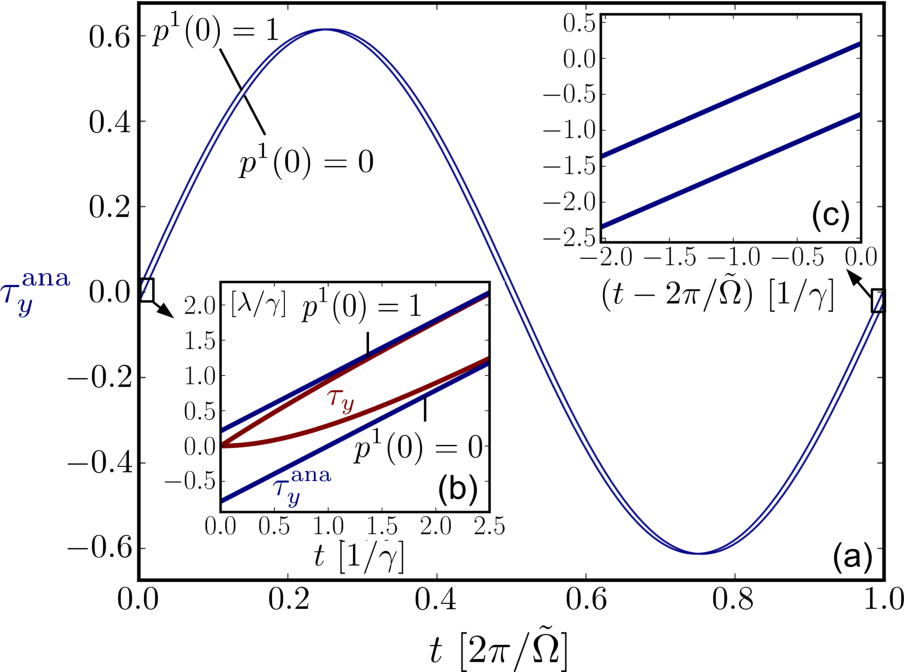
IV.4 Distortion of isospin mode vectors

The rough mean-field picture also breaks down when accounting for the backaction effect on the isospin modes vectors: the eigenvectors ${\color[rgb]{0,0,0}\mathbf{e}}_{\operatorname{eff},\alpha}$ are modified from Eq. (182) to Eqs. (178)–(180) when taking into account the finite decoherence rate $\lambda^{2}/\gamma$ . This leads to both a tilting of the qubit axis and elliptical isospin precession.

IV.4.1 Tilting of precession axis

As a first consequence, the effective precession axis $\mathbf{e}_{\operatorname{eff},0}$ acquires an additional tilting beyond the mean-field effect. This manifests as a nonzero component of $\mathbf{e}_{\operatorname{eff},0}$ along $\mathbf{e}_{\parallel}\times\mathbf{e}_{\perp}=\hat{{\color[rgb]{0,0,0}{\bm{\Omega}}}}\times\hat{{\color[rgb]{0,0,0}{\bm{\lambda}}}}$ , which is perpendicular to both the intrinsic qubit precession axis $\hat{{\bm{\Omega}}}$ and the measurement vector $\hat{{\bm{\lambda}}}$ and therefore perpendicular to $\hat{{\bm{\Omega}}}$ . By virtue of Eq. (178) this rotates the qubit axis relative to $\mathbf{e}_{\parallel}$ by an angle

\displaystyle\chi

\displaystyle\approx

\displaystyle r\frac{\lambda^{2}}{\gamma\tilde{\Omega}}\frac{\Omega\lambda p^{1}_{\operatorname{st}}}{\tilde{\Omega}^{2}}

(184)

plus higher-order corrections. This tilt becomes noticeable close to resonance, where detection is performed, as we illustrate in Fig. 10(a), where we plot the projection of ${\color[rgb]{0,0,0}{\bm{\tau}}}(t)$ onto the mean-field axis $\mathbf{e}_{\parallel}=\tilde{{\color[rgb]{0,0,0}{\bm{\Omega}}}}/\tilde{\Omega}$ . In addition to an exponential decay with the relaxation rate $1/T_{1}$ , this component acquires an additional oscillatory component for a general initial state. This simply indicates that we are looking at the component along a vector that is not the zero eigenmode of the qubit: the backaction additionally tilts the relaxation mode vector from $\mathbf{e}_{\parallel}\rightarrow\mathbf{e}_{0,\operatorname{eff}}$ through the virtual-transition terms $\propto\lambda^{2}/\gamma$ .

However, the component of ${\color[rgb]{0,0,0}{\bm{\tau}}}(t)$ along the tilted relaxation mode vector $\mathbf{e}_{\operatorname{eff},0}$ shows also an oscillation (superposed on an exponentially decaying contribution) as the red curve in Fig. 11(a) illustrates. This is an effect of the mode distortion: the plane spanned by the unit vectors $\mathbf{e}_{\operatorname{eff},1}$ and $\mathbf{e}_{\operatorname{eff},2}$ is not anymore orthogonal to $\mathbf{e}_{\operatorname{eff},0}$ . Since the precessing part of the isospin lies in this plane, the projection of the isospin ${\bm{\tau}}(t)$ on $\mathbf{e}_{\operatorname{eff},0}$ becomes oscillatory as sketched in Fig. 10(b). These oscillations are therefore damped with the dephasing rate $1/T_{2}$ , which differs from the relaxation rate $1/T_{1}$ that sets the time scale for the exponential decay of the nonoscillatory contribution. Thus, the nonorthogonality of the isospin mode vectors mixes relaxation and dephasing in a nontrivial way.

The only component of ${\bm{\tau}}(t)$ that does not oscillate for an arbitrary initial state is the one along $\tilde{\mathbf{e}}_{\operatorname{eff},0}$ as the blue curve in Fig. 10(a) shows. The reason is that the dual vector $\tilde{\mathbf{e}}_{\operatorname{eff},0}\propto\mathbf{e}_{\operatorname{eff},1}\times\mathbf{e}_{\operatorname{eff},2}$ is normal to the $\mathbf{e}_{\operatorname{eff},1}$ - $\mathbf{e}_{\operatorname{eff},2}$ plane [see definition (181)]. This normal component is also independent of the dephasing time: it simply decays exponentially with the relaxation rate $1\text{/}T_{1}$ .

However, the dual vector $\tilde{\mathbf{e}}_{\operatorname{eff},0}$ should not be confused with the zero mode $\mathbf{e}_{\operatorname{eff},0}$ : If we initially have ${\color[rgb]{0,0,0}{\bm{\tau}}}_{\operatorname{eff}}(0)\propto\tilde{\mathbf{e}}_{\operatorname{eff},0}$ , then the isospin still has a precessional component since $\tilde{\mathbf{e}}_{\operatorname{eff},0}$ is not the relaxation mode vector. If one aims to prepare the qubit in a state whose Bloch vector direction is stable under the time evolution that includes the measurement backaction, one should take

\displaystyle{\color[rgb]{0,0,0}{\bm{\tau}}}_{\operatorname{eff}}(0)

\displaystyle=

\displaystyle F\mathbf{e}_{0,\operatorname{eff}},

(185)

where $F$ is suitable real constant. ¹¹¹¹ 11 Note that ${\color[rgb]{0,0,0}{\bm{\tau}}}_{\operatorname{eff}}(0)$ differs from the initial isospin ${\bm{\tau}}(0)$ due to the initial slip (166) and therefore $F$ is not necessarily limited to the range $[-1,+1]$ . For the initial state (185), we indeed find pure exponential decay to the stationary state ${\color[rgb]{0,0,0}{\bm{\tau}}}(\infty)=\mathbf{0}$ :

\displaystyle{\color[rgb]{0,0,0}{\bm{\tau}}}(t)

\displaystyle=

\displaystyle Fe^{-t\text{/}T_{1}}\mathbf{e}_{\operatorname{eff},0}.

(186)

The above illustrates that the notion of “exciting a qubit mode” has to be treated with care due to both backaction-induced initial slip and due to mode vector distortion. Due to the initial slip discussed above, one has to prepare the qubit-sensor state [see Eq. (149), Eq. (166), and Appendix C] very carefully in order to achieve the initial condition (185).

IV.4.2 Elliptical precession

The second qualitative consequence of the distortion of the qubit modes due to the finite decoherence rate concerns the precessional motion in the $\mathbf{e}_{\operatorname{eff},1}$ – $\mathbf{e}_{\operatorname{eff},2}$ plane with normal $\tilde{\mathbf{e}}_{\operatorname{eff},0}$ . The trajectory of the isospin vector ${\color[rgb]{0,0,0}{\bm{\tau}}}(t)$ in this plane is changed from a circle to an ellipse. We illustrate this in Fig. 11(a) for an effective initial isospin ${\color[rgb]{0,0,0}{\bm{\tau}}}_{\operatorname{eff}}(0)=F\mathbf{e}_{\operatorname{eff},1}$ lying in this plane (again for a suitable real constant $F$ ). Applying Eq. (164), the evolution of the isospin can be expressed as:

$\displaystyle{\color[rgb]{0,0,0}{\bm{\tau}}}(t)$	$\displaystyle=$	$\displaystyle e^{-t\text{/}T_{2}}F\left[\cos(\tilde{\Omega}t)\mathbf{e}_{\operatorname{eff},1}+\sin(\tilde{\Omega}t)\mathbf{e}_{\operatorname{eff},2}\right]$	(187)
	$\displaystyle=$	$\displaystyle e^{-t\text{/}T_{2}}F\left[\sqrt{1-\epsilon/2}\cos\left(\tilde{\Omega}t+\frac{\pi}{4}\right)\mathbf{v}_{1}\right.$	(187)
		$\displaystyle\text{ \ \ \ \ \ \ \ \ \ }+\sqrt{1+\epsilon/2}\sin\left.\left(\tilde{\Omega}t+\frac{\pi}{4}\right)\mathbf{v}_{2}\right].$	(188)

In the rewritten form, the part in the bracket describes an elliptical motion with linear eccentricity

\displaystyle\epsilon\ =\ 2\mathbf{e}_{\operatorname{eff},1}\cdot\mathbf{e}_{\operatorname{eff},2}

\displaystyle=

\displaystyle\frac{1}{\tilde{\Omega}T_{1}}\text{ \ }=\text{ \ }r\frac{\lambda^{2}}{\gamma\tilde{\Omega}}\frac{\Omega^{2}}{\tilde{\Omega}^{2}},

(189)

which is maximal near the resonance of the sensor QD [due to $r$ , see Eq. (137)] and proportional to the scale $\lambda^{2}/\gamma$ for the decoherence rate relative to the qubit frequency $\tilde{\Omega}$ . The precession plane is spanned by two orthonormal vectors,

\displaystyle\mathbf{v}_{1,2}

\displaystyle=

\displaystyle\frac{\mathbf{e}_{\operatorname{eff},1}\pm\mathbf{e}_{\operatorname{eff},2}}{\sqrt{2\pm\epsilon}},

(190)

which are at the same time unit vectors along the principal axes of the precession ellipse as sketched in Fig. 11(b).

Equation (188) shows that the magnitudes of both principal axes shrink exponentially with rate $1/T_{2}$ . The magnitude of the isospin [green curve in Fig. 11(a)] thus oscillates around a pure exponential decay with that rate [blue curve in Fig. 11(a)]. The oscillations are a signature of the elliptical distortion of the precessional motion.

If there were no mode distortion, the above picture would be true also for slipped initial states out of the $\mathbf{e}_{1,\operatorname{eff}}$ – $\mathbf{e}_{\operatorname{eff},2}$ plane. However, due to the mode distortion arbitrary initial states must again considered with care because the projection of ${\bm{\tau}}(t)$ onto the $\mathbf{e}_{\operatorname{eff},1}$ - $\mathbf{e}_{\operatorname{eff},2}$ precession plane has an additional contribution arising from the component of ${\bm{\tau}}$ along $\mathbf{e}_{\operatorname{eff},0}$ [see Fig. 10(b)]: this causes the center of the ellipse to be shifted away from origin. This shift of the center decays exponentially towards the origin with the relaxation rate $1/T_{1}$ , which is again different from the decay rate of the precession, which is damped with the dephasing rate $1/T_{2}$ .

Relation to state purity. The discussed elliptical isospin motion reflects the exponentially damped but oscillatory decrease of the qubit-state purity due to the readout by the sensor QD. This can be roughly understood as follows. The dephasing is the strongest when the isospin and the measurement vector $\hat{{\bm{\lambda}}}$ are perpendicular to each other because this corresponds to the charge qubit electron being delocalized between the two sites. Here, small fluctuations in the detuning, induced by the stochastic switching of the SQD, then introduce a strong dephasing. By contrast, no dephasing appears when the isospin and the measurement vector $\hat{{\bm{\lambda}}}$ are collinear, i.e., when the charge qubit electron is localized in one of the QDs. This interpretation is consonant with the situation in Fig. 11(a), which shows the magnitude of the qubit Bloch vector as a function of time. The qubit Bloch vector has initially a large overlap with $\hat{{\bm{\lambda}}}$ , leading to a suppressed decay in the first quarter of a precession period $2\pi/\tilde{\Omega}$ . The oscillatory reduction of the qubit purity was anticipated also in our discussion of the exact relation (II.3),

\displaystyle\frac{d}{dt}[|{\color[rgb]{0,0,0}{\bm{\tau}}}(t)|^{2}]

\displaystyle=

\displaystyle-2{\color[rgb]{0,0,0}{\bm{\lambda}}}\cdot[{\color[rgb]{0,0,0}{\bm{\tau}}}^{0}(t)\times{\color[rgb]{0,0,0}{\bm{\tau}}}^{1}(t)].

(191)

If ${\bm{\tau}}(t)$ precesses, its charge-specific components ${\bm{\tau}}^{n}(t)$ also precess and their components along ${\bm{\lambda}}$ change in time, resulting in a nonexponential purity decay ¹²¹² 12 We note that applying Eq. (191) requires a calculation of the charge-specific isospins from the full kinetic equations (III.2.2). Using only the projections quasistationary subspace, $\mathbf{X}^{q}(t)=\left(1\ {\bm{\tau}}(t)\right)^{{\dagger}}$ , see Eq. (B.3.1), would just yield zero when inserted into Eq. (191)..

Finally, we note that these oscillations of the purity decay are not an effect of non-Markovian corrections [see Eqs. (148) and (149)] induced by the sensor QD onto the qubit by capacitive interaction $\lambda$ : they may even be reproduced by modeling the SQD charge as a classical fluctuator (see, e.g., Refs. Abel and Marquardt 2008; Neuenhahn et al. 2009). In fact, to obtain Eqs. (164) and (166), we employ a Markovian approximation with respect to the sensor on the qubit (by setting $z=0$ , see discussion in Appendix B.3.3). The oscillations of the qubit decay should also not be mistaken for coherence revivals, i.e., an increase in the purity of the qubit state. Figure 11(a) clearly shows that the magnitude of the qubit Bloch vector decreases for all times, i.e., the information is permanently transferred to the environment during the measurement process. However, the rate of information loss is nonmonotonic, which simpler approaches might not predict (see, e.g., Ref. Clerk et al. 2010). This shows most clearly that our perturbation theory goes beyond the simple “mean-field” detector picture discussed in Sec. IV.2.

V Comparison to other approaches

In this final Section we compare our results for the measurement backaction with the results of prior works. One of the central results that we obtained – the strong suppression of the measurement backaction when tuning the sensor into the Coulomb blockade regime – is surprising: One expects to underestimate the measurement backaction by a too simplified treatment which ignores cotunneling noise. We accounted for this cotunneling noise contribution (“broadening” contribution to the rates) but our result (142) revealed that it is canceled out by the coherent backaction, a renormalization effect. Such a cancellation should of course be viewed very critically and we have carefully traced its origins. It also raises the question, which physical assumptions and approximations may have caused it not to be noticed before. This is discussed here.

We first show in Sec. V.1 that semiclassical approaches can only reproduce the contributions to the decay times induced by the stochastic backaction, but they fail to account for corrections from the coherent backaction. This also quite easily happens within a standard weak-coupling Bloch-Redfield approach aimed at finding a qubit-only description as we discuss in Sec. V.2. Both these approaches are correct only under the assumption of the weak-coupling, high-temperature limit, which may experimentally be violated and does not allow the sensor QD current to be calculated. Finally, we show that our findings are in accordance with exact quantum treatments of models of decoherence due to noninteracting two-level fluctuators in equilibrium, insofar a comparison is possible.

V.1 Semiclassical stochastic approaches

A popular way to study the decoherence a qubit suffers from the coupling to its environment is a semiclassical qubit-fluctuator model Galperin et al. 2004; Ithier et al. 2005; Schriefl et al. 2006; Chirollli and Burkard 2008; Bergli et al. 2009. In this approach, the qubit is considered subjected to noise generated by a randomly switching two-level system. The basic idea is to replace the occupation number $\hat{n}$ of the SQD in the interaction Hamiltonian, $H_{I}=\hat{n}{\color[rgb]{0,0,0}{\bm{\lambda}}}\cdot\hat{{\color[rgb]{0,0,0}{\bm{\tau}}}}/2$ , by a classical random process $\hat{n}\rightarrow\xi(t)/2$ ¹³¹³ 13 We introduce a factor 1/2 for convenience to adjust the amplitude of the fluctuations to $\Delta\xi=2$ , as usually used for a random telegraph process.. Applied to our case, the SQD introduces a fluctuating effective magnetic field acting on the qubit [see Eq. (27)]:

\displaystyle H_{Q}^{\operatorname{eff}}

\displaystyle=

\displaystyle\frac{1}{2}\left({\bm{\Omega}}+\tfrac{1}{2}\xi(t){\color[rgb]{0,0,0}{\bm{\lambda}}}\right)\cdot\hat{{\color[rgb]{0,0,0}{\bm{\tau}}}}.

(192)

Since our primary interest lies in the interplay of the coherent backaction with the cotunneling-induced backaction, we can take $\Omega=0$ and drop the spin degree of freedom of the SQD electrons and therefore the effect of the Coulomb interaction in the following. Neither of these assumptions are critical for reproducing these effects (see Appendix D). The measurement then induces a dephasing of superpositions of the qubit states ${\color[rgb]{0,0,0}|}L{\color[rgb]{0,0,0}\rangle}$ and ${\color[rgb]{0,0,0}|}R{\color[rgb]{0,0,0}\rangle}$ , physically related to the double-QD electron residing either in the left or right QD. This can be characterized by the decay of the off-diagonal elements of the qubit density matrix, the visibility Bergli et al. 2009; Grishin et al. 2005; Abel and Marquardt 2008:

	$\displaystyle\left\langle\hat{\tau}_{+}(t)\right\rangle$	$\displaystyle=$	$\displaystyle\left\langle{\color[rgb]{0,0,0}\langle}L{\color[rgb]{0,0,0}\|}e^{-i\int_{0}^{t}dt_{1}H_{Q}^{\operatorname{eff}}(t_{1})}{\color[rgb]{0,0,0}\|}L{\color[rgb]{0,0,0}\rangle}\right.$		(193)
			$\displaystyle\times\left.{\color[rgb]{0,0,0}\langle}R{\color[rgb]{0,0,0}\|}e^{+i\int_{0}^{t}dt_{1}H_{Q}^{\operatorname{eff}}(t_{1})}{\color[rgb]{0,0,0}\|}R{\color[rgb]{0,0,0}\rangle}\right\rangle.$		(193)

Here, the bracket $\langle\ldots\rangle$ denotes the average over many realizations of the random process $\xi(t)$ with $\langle\xi(t)\rangle=2p^{1}_{st}$ . Splitting the qubit Hamiltonian $H_{Q}=\langle H_{Q}\rangle+\delta H_{Q}$ according to Eq. (27) into a mean-field part, $\langle H_{Q}\rangle=\frac{1}{2}p^{1}_{\operatorname{st}}{\color[rgb]{0,0,0}{\bm{\lambda}}}\cdot{\color[rgb]{0,0,0}{\bm{\tau}}}$ , and a fluctuating part, $\delta H_{Q}=\frac{1}{4}\delta\xi(t){\color[rgb]{0,0,0}{\bm{\lambda}}}\cdot\hat{{\color[rgb]{0,0,0}{\bm{\tau}}}}$ , with $\delta\xi(t)=\xi(t)-\langle\xi(t)\rangle$ and $\langle\delta\xi(t)\rangle=0$ , Eq. (193) can be recast as

\displaystyle\left\langle\hat{\tau}_{+}(t)\right\rangle

\displaystyle=

\displaystyle\left\langle e^{-\frac{i\lambda}{2}\int_{0}^{t}dt_{1}\delta\xi(t_{1})}\right\rangle.

(194)

Hence, the decay of the coherences depends only on the “amplitude” of the fluctuations, while the average of the fluctuations, $\langle\xi(t)\rangle$ , is irrelevant. This mean-field part just induces a constant shift of the qubit energy level, which has been absorbed into the average $\langle H_{Q}\rangle$ , see our discussion of the mean-field picture in Sec. IV.2.1.

For simplicity, let us first take $\delta\xi(t)$ to be a Gaussian random process. In this case, Eq. (194) can be rewritten as Bergli et al. 2009

\displaystyle\left\langle e^{\frac{-i\lambda}{2}\int_{0}^{t}dt_{1}\delta\xi(t_{1})}\right\rangle\ =\ e^{-\frac{\lambda^{2}}{8}\int_{0}^{t}dt_{1}\int_{0}^{t}dt_{2}\langle\delta\xi(t_{1})\delta\xi(t_{2})\rangle},

(195)

resulting in an exponential decay of $\left\langle\hat{\tau}_{+}(t)\right\rangle=e^{-t/T_{2}}$ . The dephasing time,

\displaystyle\frac{1}{T_{2}}\text{ \ }=\text{ \ }\frac{1}{T_{\phi}}

\displaystyle=

\displaystyle\left(\frac{\lambda}{2}\right)^{2}\frac{S_{\delta\xi}(0)}{2},

(196)

can be related to the noise power spectrum $S_{\delta\xi}(\omega)$ of the Gaussian random process $\delta\xi(t)$ Bergli et al. 2009,

\displaystyle S_{\delta\xi}(\omega)

\displaystyle:=

\displaystyle\int_{-\infty}^{+\infty}d\tau e^{-i\omega\tau}\langle\delta\xi(0)\delta\xi(\tau)\rangle,

(197)

where we used that the correlator $\langle\delta\xi(t_{1})\delta\xi(t_{2})\rangle$ only depends on the time difference $\tau=t_{2}-t_{1}$ because a Gaussian random process is time-translational invariant. We emphasize that the relation (195) holds exactly for a Gaussian process, whose entire statistics is fixed by two-point correlation functions.

For a general random process, however, higher-order time correlators may contribute to Eq. (195) Galperin et al. 2004; Bergli et al. 2009; Makhlin and Shnirman 2004 and therefore the spectral function is not sufficient to characterize a random process completely. A prominent example is a Poisson process inducing random telegraph noise. Such a process would actually be a better model for a capacitively coupled QD stochastically switching its occupation due to tunneling processes. Random telegraph noise has also been extensively studied to explain the origin of flicker ( $1/f$ ) noise in superconducting qubits Ithier et al. 2005; Bergli et al. 2009; Shnirman et al. 2005; Schriefl et al. 2006; Galperin et al. 2004 and Gaussian noise in semiconductor QDs Berthelot et al. 2010; Kuhlmann et al. 2013. This noise results from an ensemble of fluctuating background charges, each of which may be compared with our sensor QD, except that they do not carry a current on average. The non-Gaussian behavior of the Poisson process comes to light only if a few fluctuators dominate the decoherence of the qubit state, which entails a nonexponential decay of the coherences Bergli et al. 2009; Paladino et al. 2002; Abel and Marquardt 2008; Neuenhahn et al. 2009 and even coherence revivals have been predicted Neuenhahn et al. 2009; Abel and Marquardt 2008.

The impact of charge fluctuations of an individual QD have also been modeled by classical random telegraph process Bergli et al. 2009; Itakura and Tokura 2003. In general, $\delta\xi$ switches between two values $\delta\xi_{u}$ (upper), and $\delta\xi_{l}$ (lower) with different switching rates $1/\tau_{l}$ for $\delta\xi_{u}\rightarrow\delta\xi_{l}$ , and $1/\tau_{u}$ for $\delta\xi_{l}\rightarrow\delta\xi_{u}$ . This gives rise to different probabilities $p_{u}$ to find the value $\delta\xi_{u}$ , and $p_{l}$ to find the value $\delta\xi_{l}$ , respectively. In the weak-coupling limit, $\lambda\ll\gamma=1/\tau_{u}+1/\tau_{l}$ , it turns out that the dephasing is still exponential and the dephasing rate reads as ¹⁴¹⁴ 14 We adjusted the notation in Ref. Itakura and Tokura 2003 to our notation by replacing $1/\tau_{0}=1/\tau_{u}+1/\tau_{l}=\gamma$ and $J_{T}\rightarrow\lambda/2$ .:

\displaystyle\frac{1}{T_{2}}

\displaystyle\approx

\displaystyle[1-(p_{u}-p_{l})^{2}]\frac{(\lambda/2)^{2}}{\gamma}.

(198)

Identifying $p_{u}\rightarrow p^{1}_{\operatorname{st}}$ and $p_{l}\rightarrow p^{0}_{\operatorname{st}}$ with the stationary occupation probabilities of the SQD for our case and noting $(\hat{{\bm{\lambda}}}\cdot\mathbf{e}_{||})^{2}=1$ for $\Omega=0$ , Eq. (198) reproduces the the dephasing rate (176), which we obtained in the high-temperature limit.

Yet, in the classical fluctuator model, we have not explicitly assumed high temperatures. Thus, if one naively extends the above result to include cotunneling corrections, one gets a faulty result. The cotunneling changes the occupation probabilities $p^{0}_{\operatorname{st}}$ and $p^{1}_{\operatorname{st}}$ and the switching rate $\gamma$ , but there is no way in which additional coherent backaction terms could appear [see the transition factor $r$ , Eq. (137)]. As a consequence, one might overestimate the qubit dephasing rate at the onset of Coulomb blockade. In addition, the classical approach does also not account for the dissipative backaction, which is less important for the dephasing times as compared to the coherent backaction ¹⁵¹⁵ 15 The reason is that the dissipative backaction does not affect the coupling between the quasistationary and decay modes [see Eqs. (III.3.3) – (III.3.3)]..

The reason why the above classical approach is not able to reproduce the coherent backaction is that the electron number $n$ is a classical variable with a definite value at each instant of time, meaning the SQD is fluctuating between the states $|0\rangle\langle 0|$ and $|1\rangle\langle 1|$ , where $|n\rangle$ denotes the SQD state with $n$ electrons on it. In this way, it can only produce the stochastic backaction. Quantum coherences $|0\rangle\langle 1|$ and $|1\rangle\langle 0|$ involved in virtual processes of the SQD (quantum fluctuations), which play a role during the tunneling, are disregarded here. However, as we illustrate in Appendix D, these coherences – included in our calculation – are crucial for obtaining the coherent backaction. (Note that despite this, such coherences can not appear in the real quantum state, the relevant density operator $\rho$ [see Eq. (12)] due to charge conservation.) It turns out that the related quantum fluctuations induce an additional “phase kick” while a charge transition in the SQD takes place. This phase shift partially compensates the phase shift from the stochastic backaction while the SQD is in a specific charge state. This makes plausible why quite generally one may expect a coherent backaction that mitigates measurement backaction when employing a quantum sensor for the indirect detection of a qubit. Thus, a purely classical understanding of the indirect measurement backaction due to a sensor QD is incomplete.

V.2 Bloch-Redfield approach

Another frequently employed method to study decoherence is the Bloch-Redfield approach Redfield 1957; Breuer and Petruccione 2002, also in the context of qubits Chirollli and Burkard 2008; Ithier et al. 2005. In the original presentation Redfield 1957, this approach is first developed for a semiclassical ¹⁶¹⁶ 16 In Redfield’s notation in Ref. Redfield 1957, the random perturbation is for our model given by $G(t)=\frac{1}{2}\xi(t){\color[rgb]{0,0,0}{\bm{\lambda}}}\cdot\hat{{\color[rgb]{0,0,0}{\bm{\tau}}}}$ . and after this also for a quantum perturbation. In both cases, one considers the limit of weak coupling between a quantum system and its environment and an additional Born-Markov approximation is made. Importantly, the approach generally predicts an exponential decay into a stationary state irrespective of the statistics of the environmental fluctuations. The corresponding relaxation matrix of the reduced density matrix is furthermore related to the noise power spectrum of the perturbation.

V.2.1 Stochastic backaction in spectral function

For our case, the Bloch-Redfield approach confirms the dephasing rate (196) also within a quantum treatment: one simply has to replace in Eq. (197) the classical average $\langle\delta\xi(t)\delta\xi(t+\tau)\rangle$ by the quantum-ensemble average:

\displaystyle S_{\delta\hat{n}}(\omega)

\displaystyle:=

\displaystyle\int_{-\infty}^{+\infty}d\tau e^{-i\omega\tau}4\left\langle\delta\hat{n}(t)\delta\hat{n}(t+\tau)\right\rangle.

(199)

For an indirect readout model of interest here, one treats the SQD as a noninteracting two-level quantum system in contact with a thermal reservoir. Applying the results of Ref. Shnirman et al. 2005 for a single fluctuator, the spectral function reads ¹⁷¹⁷ 17 To compare with Eq. (7) of Ref. Shnirman et al. 2005, we note that for our model there is no direct hybridization $\Delta_{j}=0$ between the orbital levels of the SQD, i.e., $\cos(\theta_{j})=1$ , and $\sin(\theta_{j})=0$ . Furthermore, the relaxation rate $\Gamma_{1,j}$ to the stationary state is identified with $\gamma$ here.

\displaystyle S_{\delta\hat{n}}(\omega)

\displaystyle=

\displaystyle[1-(p^{1}_{\operatorname{st}}-p^{0}_{\operatorname{st}})^{2}]\frac{2\gamma}{\gamma^{2}+\omega^{2}}

(200)

leading to Eq. (198) when inserting $S_{\delta\hat{n}}(\omega=0)$ into Eq. (197). Hence, also the Bloch-Redfield approach – even accounting for a quantum environment – does not reproduce the coherent backaction and may therefore be applied only in the high-temperature limit to derive dephasing and relaxation times.

V.2.2 Difficulty of capturing dissipative and coherent backaction

The reason why the Bloch-Redfield approach fails to account for the dissipative and coherent backaction is not specific to this approach. It is rather a problem that appears in principle for any procedure that tries to treat the sensor in an indirect measurement setup as a given environment without a nonequilibrium dynamics of its own. Such an approach always needs to make some assumptions about the sensor density operator, which, as we have seen, does not seem to have a simple structure allowing for an educated guess based on general physical principles. This means that one should simply calculate the joint quantum state of sensor QD and qubit, which is what we have done. It is, however, instructive to further understand the problems encountered when one tries to avoid this by making (too) simple approximations of this joint state.
(i) The Bloch-Redfield approach (as well as many other density-operator approaches) applied in the weak-coupling limit involves a factorization assumption Koller et al. 2010 for the state of the qubit and its environment (here the sensor QD plus the reservoir): $\rho_{\operatorname{tot}}(t)\approx\rho_{Q}(t)\otimes\rho_{SR}(t)$ . The factorization assumption ignores the dissipative backaction valid only in the high-temperature limit. Otherwise, the dissipative backaction leads to a nonzero stationary qubit Bloch vector that reflects the nonfactorisability of the qubit-environment state even in the stationary limit. By contrast, to find the decoherence rates in the long-time limit $t-t_{0}>1/\Gamma$ , the factorization assumption may still work.
(ii) The next critical point is then to find a proper description for the unknown evolution $\rho_{SR}(t)$ of the environment. An assumption frequently made is that the qubit environment is in a stationary state, $\rho_{SR}(t)=\rho_{SR,\operatorname{st}}$ , for example, an equilibrium state. However, stationarity of the entire qubit environment (SQD plus electrodes) is actually never reached whenever a measurement is performed, for which the electrodes must be held at finite bias to produce a nonzero measurement current. Here one should be careful to note that while the reduced sensor QD density operator may become stationary after some time, this is not true for the joint SQD-electrode state. In our approach, the reduced sensor-qubit system can become stationary after eliminating the electrodes, which are stationary.
(iii) Even if we further simplify the problem and assume zero bias voltage (e.g., to compute the measurement backaction in linear response) and $\rho_{SR,\operatorname{eq}}$ is stationary, then it is still difficult to compute the equilibrium state $\rho_{SR,\operatorname{eq}}$ since the sensor QD is a strongly interacting system. Naive assumptions made about $\rho_{SR,\operatorname{eq}}$ are prone to errors. Consider for instance the approximation $\rho_{SR,\operatorname{eq}}=\rho_{S,\operatorname{st}}\otimes\rho_{R,0}$ , where $\rho_{S,\operatorname{st}}$ denotes the stationary SQD state and $\rho_{R,0}$ is the grand-canonical equilibrium state of the reservoirs. (One may be inclined to make this approximation since weak coupling $\Gamma$ often implies such a factorization.) If we use this state and average the two-point charge correlator in Eq. (199), this involves only charge-diagonal SQD states $|0\rangle\langle 0|$ and $|1\rangle\langle 1|$ – similar to the semiclassical approach of Sec. V.1. What goes wrong here is that $\rho_{S,\operatorname{st}}\otimes\rho_{R,0}$ is not the correct equilibrium state if we go beyond the lowest-order $\Gamma$ approximation in the tunneling. For larger $\Gamma$ , the hybridization between both systems cannot be neglected any more Koller et al. 2010. During tunneling processes the total system can be in virtual intermediate states involving sensor QD coherences $|0\rangle\langle 1|$ and $|1\rangle\langle 0|$ and corresponding charge coherences in the electrode. These intermediate virtual states explicitly appear in the calculation of the coherent backaction (see Appendix D). Thus, even the quantum-ensemble averaging procedure that brings us from Eq. (199) to Eq. (200) misses the coherent backaction since it relies on a weak-coupling expansion between SQD and electrodes.
This explains why for an indirect weak measurement setup, the procedure employed in this paper and also in Refs. Shnirman and Schön 1998; Makhlin et al. 2001 seems unavoidable. By integrating out the electrodes first one incorporates their effect on the joint sensor-qubit system. As we have seen, this reveals that the qubit experiences a stochastic, dissipative, as well as a coherent backaction effect. This problem of describing the nonstationary environment is specific to indirect measurement setups and not encountered when the qubit is directly coupled to, e.g., a stationary environment. This is the case, for example, for a bath of harmonic oscillators as in the spin-boson model Paladino et al. 2008; Shnirman et al. 2002; Chirollli and Burkard 2008, where the environment may indeed be described by a stationary equilibrium state. Yet, previous studies for other types of environments also show that the approximations made to integrate out the entire qubit envronment can be too crude, including both a spin-boson model Gutmann et al. 2005 and a driven two-level fluctuator Gassmann et al. 2002. In particular, Ref. Gassmann et al. 2002 explicitly compares results for different levels of approximations showing the breakdown of Markov and secular approximation beyond the weak qubit-environment coupling.

V.3 Nonperturbative quantum solutions

Our study indicates that renormalization effects, based on quantum coherences between the qubit and its detector, are vital for the description of the measurement backaction even in the weak-coupling limit. We next compare our results to prior studies that treat the qubit decoherence arising from single fluctuators coupled to fermionic reservoirs fully quantum-mechanically.

Such studies employ various approaches, such as an exact numerical evaluation of the visibility (193) using electrodes of finite size Abel and Marquardt 2008, a Heisenberg equation-of-motion technique Paladino et al. 2002, or a Keldysh path-integral formalism Grishin et al. 2005; Paladino et al. 2002. All these approaches are nonperturbative both in the measurement interaction $\lambda$ and the sensor tunneling $\Gamma$ . However, in contrast to our model these studies are limited to noninteracting fluctuators (here: the SQD) in equilibrium with a single reservoir. Thus, they cannot access the situation of a (nonequilibrium) signal current through the fluctuator, an essential aspect of the indirect detection that we do consider. Moreover, they only consider qubit energy splittings along the measurement vector, in our notation $H_{Q}=\Omega\hat{\tau}_{z}/2$ , that is, they only study pure dephasing in which the qubit Bloch vector has no precessional motion. This leads to drastic simplifications employed in the derivation of these approaches which limit their applicability.

References Abel and Marquardt 2008; Neuenhahn et al. 2009 highlight coherence revivals for the short-time transients in the strong measurement regime $\lambda\gg\Gamma$ . This nonexponential decay reflects the non-Gaussian statistics of the quantum telegraph process. Moreover, these studies also find oscillatory corrections to the dephasing even in the weak-measurement regime $\lambda<\Gamma$ in agreement with our work (see Fig. 11). The dependence of the dephasing rate on the level position is not reported and thus cannot be compared.

In Ref. Paladino et al. 2002, a path integral method is used to study the qubit decoherence due to two-level fluctuators. Their dephasing rate also includes terms containing the real part of the digamma function $\psi$ , which determines the renormalization function $\phi$ [Eq. (48)]. It appears both in the cotunneling rates [see in Eq. (45)] as well as in the coherent backaction [Eq. (53)]. In contrast to Ref. Paladino et al. 2002, our expressions depend on the derivative $\phi^{\prime}$ , which is arises from our expansions in $\lambda$ and $\Gamma$ . However, a direct comparison is not possible because tangible results of Ref. Paladino et al. 2002 are actually given only for the sequential tunneling regime where renormalization effects are neglected ¹⁸¹⁸ 18 This is a consequence of the approximation $K_{2,j}(\lambda)\approx K_{2,j}(0)$ employed below Eq. (3) in Ref. Paladino et al. 2002..

Reference Grishin et al. 2005 also uses a path-integral approach and considers also the case when the QD level $\varepsilon$ is tuned strongly away from resonance $|\varepsilon-\mu|/T\gg 1$ . Expanding their result (Eq. (15) of Ref. Grishin et al. 2005) for the long-time limit of the dephasing rate in the weak-measurement limit, we obtain ¹⁹¹⁹ 19 We express the parameters $g$ and $\tilde{\varepsilon}$ in Ref. Grishin et al. 2005 in terms of our notation as $g=\lambda/\Gamma$ and $\tilde{\varepsilon}=2\varepsilon/\Gamma$ .:

\displaystyle\frac{1}{T_{2}}

\displaystyle=

\displaystyle\frac{T}{4\pi}\frac{\lambda^{2}\Gamma^{2}}{(\varepsilon-\mu)^{4}}+O\left((\lambda/\Gamma)^{4}\right).

(201)

Thus, the dephasing rate drops algebraically in the fourth power with the level position. This is consistent with our results in the sense that also here the decoherence does not scale as expected from the cotunneling noise. In our case, we were only able to show that the algebraic scaling in $1/(\varepsilon-\mu)$ is suppressed at least to the second power (see Sec. III.4.1). However, our analysis revealed the physical origin of this behavior by identifying what cancels the expected cotunneling noise contribution, namely the coherent backaction. Note that the result (201) does not rely on the high-temperature assumption $\Gamma/T\ll\lambda/\Gamma$ as in our case, which is why their result can be expanded in orders $\lambda/\Gamma$ while accounting also for higher-order tunneling corrections [e.g., $O(\Gamma^{3}/T^{2})$ and higher, see Appendix B.4]. This implies that to compare concretely with their result (201), we would have to include higher-order tunneling terms, which, however, we do not expect to restore power laws with lower exponents. This is challenging for our model since we account for Coulomb interactions and nonequilibrium conditions. This is beyond the scope of the present paper.

In summary, various aspects of our assumptions and findings seem to be in accordance with previous approximate as well as exact quantum-mechanical treatments and shed new light on them. Our study extends these approaches by simultaneously dealing with a nonstationary, nonequilibrium, Coulomb-blockaded sensor QD (fluctuator), which is fully quantum-correlated with the qubit (non-factorizing density operator $\rho$ , virtual off-diagonal charge coherences during tunneling). The latter leads to the coherent backaction as an integral part of the total backaction together with stochastic and dissipative backaction, leading to the cancellation of cotunneling noise.

VI Summary and Outlook

We studied an indirect detection setup, in which a charge qubit is capacitively probed ( $\lambda$ ) by a sensor quantum dot (SQD). The SQD is in turn tunnel coupled ( $\Gamma$ ) to electrodes in which the time-dependent conductance is measured. Electrons in the sensor QD occupy a single quantized orbital in which they strongly interact.

Kinetic equations. We considered the weak-tunneling, weak-measurement limit $\Gamma/T\ll\lambda/\Gamma\ll 1$ , in which quantum fluctuation effects are important on the time scale of the qubit-sensor interaction. We derived a kinetic equation [Eq. (III.2.2)] by integrating out the current-carrying electrodes to obtain an effective theory for the composite qubit-SQD system. This revealed three types of backaction on the qubit: (i) a stochastic backaction due to random fluctuations of the qubit detuning, (ii) a dissipative backaction (coefficient $c$ ), the flip side of the modulation of the sensor tunnel current by the qubit, and (iii) a coherent backaction due to the level renormalization of the composite qubit-SQD system (coefficient $\kappa$ ).

We showed the importance of the effects of single-electron tunneling (SET), as well as its cotunneling broadening and level-shift corrections. We also included the leading non-Markovian correction from the electrodes induced by the tunnel coupling ( $\Gamma$ ) to the SQD (linear kernel frequency dependence). Moreover, our approach captures all non-Markovian effects introduced by the sensor QD on the qubit subsystem, which are mediated by the capacitive interaction.

Suppression of cotunneling-induced backaction. By rewriting the kinetic equation in the basis of quasistationary and decay modes (defined by the $\lambda=0$ limit), we found that the interplay of these types of backaction leads to a nontrivial cancellation; whereas the dissipative backaction ( $c$ ) independently couples these modes, the stochastic backaction and coherent backaction ( $\kappa$ ) partially cancel. In particular, the change in the stochastic backaction due to cotunneling broadening is canceled by the coherent backaction [Eq. (137)]. The expected algebraic decay $\propto 1/(\varepsilon-\mu_{r})$ of the backaction (determining the decoherence rates) is thus suppressed, implying that the actual power law must at least have a higher exponent. Experimentally, this is important since it indicates that a SQD can be switched off by applying a gate voltage better than expected. By identifying the underlying physics, we suspect this to be a crucial difference with the backaction of sensors with dense level spectra, such as single-electron transistors. Thus, the less-than-expected backaction due to the coherent backaction is beneficial for switching the sensor on / off, provided one takes care to prepare sensor state to avoid initial slip errors (see next paragraph).

Initial slip. We derived effective equations for the reduced qubit density operator [Eq. (148)], which are exact relative to the kinetic equations (III.2.2). In particular, we keep all non-Markovian effects induced by the sensor and account for a slip of the initial condition [Eq. (149)]. This slip depends on both the initial sensor QD state and the initial quantum correlations with the sensor QD. It is important for the long-time qubit evolution and thus the sensor QD needs also to be considered as part of the dynamical quantum circuit. The dynamical state of the sensor QD is relevant for qubit error propagation, e.g., the initial slip may introduce errors even for perfectly prepared qubit initial states. This provides a concrete example for errors usually phenomenologically introduced in quantum-error correction. Such a sensor QD cannot be considered (without further evidence) as a “black box” in a quantum circuit which is merely characterized by static parameters (e.g., relaxation and dephasing times). This is different from the treatment of the macroscopic electrodes coupled to the sensor QD. The electrodes, in which the current measurement is performed, can instead be assumed to be stationary, which eliminates initial-slip effects on qubit-SQD system (provided initial quantum correlations are neglected).
High-temperature limit. Specializing to the high-temperature limit $\Gamma/T\rightarrow 0$ and to times larger than the SQD relaxation time $1/\Gamma$ , we obtained the qubit evolution [Eq. (165)], which neglects non-Markovian effects induced by the sensor QD. We connected dephasing and relaxation times $\propto\lambda^{2}/\Gamma$ with the component of the measurement vector ${{\bm{\lambda}}}$ along the mean-field qubit axis $\tilde{{\bm{\Omega}}}$ and perpendicular to it, respectively. We demonstrated the importance of the initial slip $\propto\lambda/\Gamma$ [Eq. (166)] even in this simplest limit: the set of initial states of the qubit-SQD system without slip is only a subset of zero measure. Generally, the magnitude of the slip increases the “less factorizable” the qubit-SQD state is and the “more nonstationary” the sensor QD is before the detection is started. Due to the latter, the initial slip should be reckoned with in particular when the sensor QD is initialized in a fixed charge state. This happens, for example, when switching the sensor off by tuning the gate voltage far away from resonance or by reducing the tunnel coupling $\Gamma$ to the electrodes. By contrast, switching off the capacitive interaction $\lambda$ leads to an initially stationary and factorizable state, which is favorable for avoiding an initial slip. This difference in the backaction between various parameters for switching off a sensor QD is an important experimental implication of our study. The need to control not only the qubit but also the readout device carefully may not only be a nuisance for engineering quantum circuits but could also provide additional means of controlling qubits. For example, one could consider to switch the SQD during the readout to another readout point to compensate for manipulation errors detected in a weak measurement process.
Mode distortion. The analysis of the isospin dynamics showed that additionally the qubit eigenmode vectors are distorted due to the small but finite value of the decoherence rates $\sim\lambda^{2}/\Gamma$ . This corrects the simple mean-field picture, in which the qubit axis $\tilde{{\bm{\Omega}}}={\bm{\Omega}}+p^{1}_{\text{st}}{\bm{\lambda}}$ is only influenced by the average occupation of the SQD. The distortion reflects the breakdown of the secular approximation – often made in derivations – because the capacitive coupling $\lambda$ can be of the same order as the internal qubit splitting $\Omega$ . Importantly, the distortion must be included to satisfy an isospin sum rule that follows from the conservation of the isospin by the tunneling of sensor electrons Hell et al. 2014; Salmilehto et al. 2012. The distortion is thus enforced by a general principle. The experimentally relevant consequence of this distortion for the qubit evolution is two-fold: first, the usual circular Bloch-vector precession becomes slightly elliptical, with a shape that is not altered in time as the size shrinks with dephasing rate $1/T_{2}$ . Second, this “precession plane” is not orthogonal any more to the “relaxation axis,” along which the Bloch vector decays with the relaxation rate $1/T_{1}$ . The relaxation axis is moreover slightly tilted relative to the mean-field axis $\tilde{{\bm{\Omega}}}$ . Finally, the projections of the isospin on the mean-field axis, the relaxation axis, and the precession plane all show a superposition of relaxation and precessional dephasing motion. The measurement backaction thus mixes the effects of relaxation and dephasing, even in this simple Markovian limit. This effect may generally appear in indirect-coupling setups, which are typical for detection setups.
The tilting of the qubit modes is related in a broader context to the concept of “gauge qubits” Kribs and Poulin 2013: two physically distinct qubits can be each subject to strong decoherence but the joint Hilbert space formed by both qubits may contain a two-level subsystem with low decoherence. Locating such subsystems is interesting for developing strategies for quantum-error correction. In our case, the qubit mode tilting reflects an “admixing” of the sensor QD degrees of freedom to the low-decoherence subspace, which mostly overlap with the qubit degrees of freedom. This mixing can be strongly enhanced when the coupling of the quasistationary and decay modes becomes stronger, which effectively happens, e.g., due to enhanced quantum-fluctuation effects at lower temperatures. Investigating this mixing further would therefore be interesting also in the context of quantum-error correction strategies.

Comparison with other approaches. We compared the above results at various points with existing approaches and explained why potential differences are expected within their validity:

(a) Semiclassical stochastic approaches cannot capture the coherent backaction because the starting assumption of classical charge fluctuations on the sensor QD already excludes relevant quantum coherences of the qubit-sensor density operator. Including these into the description leads to additional “phase kicks” that counteract the stochastic “phase kicks.” Both together, when averaged, lead to a mitigated decoherence. It thus seems that one should quite generally reckon with coherent backaction, which can mitigate the measurement backaction when employing a quantum-dot sensor for the indirect detection of a qubit.

(b) Density operator approaches that try to integrate out the sensor together with the attached electrodes run into problems as well because one needs to “guess” the time-dependent, current-carrying sensor state as well as the quantum correlations with the qubit. These can lead to non-Markovian behavior and affect the initial slip of the qubit. All of this is systematically calculated in our approach. The more advanced approach of Ref. Emary 2008, which first calculates the nonequilibrium SQD state in the absence of the qubit (an approximation carefully pointed out in Ref. Emary 2008), misses both the dissipative and coherent backaction. Extending such an approach, e.g., to include cotunneling broadening would thus lead to inconsistencies since only one part of two canceling effects is taken into account.
(c) Nonperturbative quantum solutions of related models agree with the cancellation in the backaction we found here as does a separate calculation for a noninteracting limit of our model ( $U=0$ ).
(d) It is also interesting to compare with prior studies not aiming at sensor backaction. In particular, Ref. Braggio et al. 2006 highlighted the importance of a competition of next-to-leading-order effects and non-Markovian corrections, which are closely related to the non-Markovian corrections of the first type affecting the dissipative switching rates (54) discussed in Sec. III.2.4. However, what is imporant here are non-Markovian corrections of the second type affecting the coherent backaction. We stress that although these non-Markovian corrections give an important part of the coherent backaction, they are not identical to it: the coherent backaction already arises in the stationary limit that we studied in Ref. Hell et al. 2014 where non-Markovian effects can be neglected. In this way, we see that the general line of thought emphasized in Ref. Braggio et al. 2006 extends to the coherent backaction, which is also a second-order effect, namely first order both in the tunneling ( $\Gamma$ ) and the measurement interaction ( $\lambda$ ).
Outlook. All this shows that the coherent backaction and other quantum fluctuation effects (cotunneling, level renormalization) are intrinsic effects of a quantum sensor: they can neither be “added” or “controlled” independently in an experiment, nor should they be neglected in a calculation. In view of the above, further studies that can address the experimentally relevant lower temperature dynamics of weak measurements using quantum-dot sensors are necessary. We expect the qualitative effects that we identified to be present and quantitatively stronger under experimental conditions where, e.g., the capacitive interaction and tunnel coupling may not be weak anymore (e.g., because of the trade-off between a significant current signal and low backaction). Besides the commonly discussed relaxation and dephasing backaction, also the qubit initial slip, nonorthogonal mode distortion, and sensor-induced memory effects will be enhanced, neither of which has received much attention so far.

Acknowledgements.

We acknowledge stimulating discussions with H. Bluhm, L. Schreiber, J. König, V. Meden, C. Klöckner, D. Kennes, and P. Samuelsson. We thank A. Braggio for helpful feedback on the preprint version. We are grateful for support from the Alexander von Humboldt foundation.

Appendix A Importance of non-Markovian corrections induced by the electrodes

In this Appendix, we explain how to account for non-Markovian corrections arising from the memory induced by the electrodes on the qubit-sensor subsystem and illustrate their importance for a correct description of the detector backaction. One should clearly distinguish from this further non-Markovian behavior induced by the SQD – with the effect of the electrodes incorporated – on the qubit subsystem. This is discussed separately in Appendix B.3.3. In Appendix A.1, we show how the non-Markovian corrections due to the electrodes can be incorporated within the real-time diagrammatic formalism based on a perturbative weak-tunneling ( $\Gamma$ ) expansion. Within the leading non-Markovian correction included in this paper, the kinetic equation remains a time-local and first-order differential equation for the density operator. Based on this, we then perform the weak-measurement expansion. In Appendix A.2, we show that neglecting the non-Markovian correction leads to a violation of the positivity of the SQD-qubit density operator and to an overestimation of the measurement backaction. These unphysical features are removed when the leading non-Markovian correction is included.

A.1 Incorporating non-Markovian effects in real-time diagrammatics

In Ref. Hell et al. 2014, we started from a kinetic equation for the reduced density operator $\rho(t)$ of the joint system of SQD plus qubit, obtained in the standard way by integrating out the electrodes’ degrees of freedom:

\displaystyle\dot{\rho}(t)

\displaystyle=

\displaystyle-iL_{QS}\rho(t)+\int_{0}^{t}dt^{\prime}W(t-t^{\prime})\rho(t^{\prime}).

(A.1)

Here, $L_{QS}\bullet=[H_{Q}+H_{S}+H_{I},\bullet]$ is the internal Liouvillian of the reduced system with “ $\bullet$ ” denoting the operator the Liouvillian acts on. The effects of the electrodes are incorporated in the kernel $W$ , which we evaluated using the real-time diagrammatic approach Schoeller 2009; Leijnse and Wegewijs 2008. In Ref. Hell et al. 2014, we were only interested in the stationary solution of Eq. (A.1), $\rho(t)=\rho_{\operatorname{st}}$ , which obeys $\dot{\rho}_{\operatorname{st}}=0$ . This solution depends only on the time-integrated kernel $\int_{0}^{t}dt^{\prime}W(t-t^{\prime})=\int_{0}^{t}d\tau W(\tau)$ . In the long-time limit $t\rightarrow\infty$ , when the stationary state is approached, the time-integrated kernel is given by the zero-frequency limit of the Laplace transform

\displaystyle W(z)

\displaystyle=

\displaystyle\int_{0}^{\infty}d\tau e^{iz\tau}W(\tau).

(A.2)

Hence, the exact $\rho_{\operatorname{st}}$ is the same as the stationary solution of the approximate, time-local Markovian kinetic equation,

\displaystyle\frac{d\rho}{dt}(t)

\displaystyle=

\displaystyle(-iL_{QS}+W)\rho(t),

(A.3)

with $W=W(z=i0)$ .

Weak-tunneling expansion. Yet, in the present paper, we study the nonstationary time evolution of the qubit-sensor density operator $\rho(t)$ and we show now that this implies that memory effects induced by the electrodes through the kernel $W$ have to be included. We will refer to all the effects of the frequency dependence of $W(z)$ , Eq. (A.2), as non-Markovian corrections induced by the electrodes [even when effectively a time-local equation results, see Eq. (A.7)]. An approach to include such corrections within the real-time diagrammatic formalism has been given in Ref. Splettstoesser et al. 2010, and applied to study decay rates in Refs. Contreras-Pulido et al. 2012; Schulenborg et al. 2014. The basic idea is to perform a Taylor expansion of $\rho(t^{\prime})$ in the integral in Eq. (A.1) around time $t$ ,

\displaystyle\rho(t^{\prime})

\displaystyle=

\displaystyle\sum_{n=0}^{\infty}\frac{1}{n!}\frac{d^{n}\rho(t)}{dt^{n}}(t^{\prime}-t)^{n},

(A.4)

and to subsequently perform the integration over $t^{\prime}$ . This results in a well-defined expression if the kernel decays faster than any polynomial in $t-t^{\prime}$ , which is usually fulfilled because the kernel decays exponentially $W(t-t^{\prime})\sim e^{-(t-t^{\prime})/\tau_{C}}$ on the time scale of the inverse temperature $\tau_{C}\sim 1/T$ ²⁰²⁰ 20 The correlation time is set by the time dependence of the contraction functions in the diagrammatic expansion (reservoir correlation functions), which drop on the time scale of the inverse temperature $1/T$ , see Eqs. (93) and (100) in Ref. Saptsov and Wegewijs 2014. Note that the contribution from the stationary state $\rho_{\operatorname{st}}$ just vanishes, i.e., $W(t-t^{\prime})\rho_{\operatorname{st}}=0$ for any time $t^{\prime}$ ..

If we consider only times $t\gg\tau_{c}$ , one may compute $\int_{0}^{t}dt^{\prime}W(t-t^{\prime})(t^{\prime}-t)^{n}=\int_{0}^{t}d\tau W(\tau)(-\tau)^{n}$ by replacing $t\rightarrow\infty$ on the right-hand side since all contributions from $\tau>t$ are negligibly small. Taking advantage of the Laplace transform (A.2), we obtain from Eq. (A.1)

\displaystyle\frac{d\rho(t)}{dt}

\displaystyle=

\displaystyle-iL_{QS}\rho(t)+\sum_{n}\frac{1}{n!}\partial^{n}W\frac{d^{n}\rho(t)}{dt^{n}},

(A.5)

with the $n$ th derivative of the Laplace-transformed kernel (A.2) at zero frequency with respect to $-iz$ :

\displaystyle\partial^{n}W

\displaystyle=

\displaystyle\left.\frac{\partial^{n}W(z)}{\partial(-iz)^{n}}\right|_{z=i0}.

(A.6)

To include the leading-order non-Markovian corrections, we truncate the sum on the right-hand side of Eq. (A.5) and keep only the terms with $n\leqslant 1$ . This yields the following time-local differential equation of first order in time:

\displaystyle\frac{d\rho(t)}{dt}\ =\ \frac{1}{\mathbbm{1}-\partial W}(-iL_{QS}+W)\rho(t)\ =\ -iL\rho(t),

(A.7)

whose solution can be written as

\displaystyle\rho(t)

\displaystyle=

\displaystyle e^{-iLt}\rho(0)

(A.8)

for initial state $\rho(0)$ . When dropping the non-Markovian correction $1/(\mathbbm{1}-\partial W)$ in Eq. (A.7), one recovers the Markovian generator of Eq. (A.3).

We next show that this solution with $L$ defined through Eq. (A.7) accounts for all non-Markovian effects up to $O(\Gamma^{2}/T)$ provided one is seeking for exponential solutions of Eq. (A.5). We do not discuss algebraic or logarithmic time dependencies here, which may also appear Pletyukhov et al. 2010. Thus, let us substitute the exponential ansatz

\displaystyle\rho(t)

\displaystyle=

\displaystyle e^{At}\rho(0),

(A.9)

into Eq. (A.5). We obtain the following equation for $A$ :

\displaystyle A

\displaystyle=

\displaystyle-iL_{QS}+W+(\partial^{1}W)A+\ldots\text{ }.

(A.10)

When all derivatives $\partial^{n}W$ are dropped from the above equation, we recover the Markovian generator $A=-iL_{QS}+W$ . Non-Markovian corrections therefore enter through terms $\sim\partial^{n}W$ that capture the frequency dependence of the kernel Braggio et al. 2006; Flindt et al. 2008; Flindt et al. 2010.

Equation (A.9) shows that the derivatives of the density operator scale as $d^{n}\rho/dt^{n}\sim A^{n}\sim\Gamma^{n}$ since $L_{QS}\sim\Delta\ll\Gamma$ and $W\sim\Gamma$ here. As a consequence, the expansion (A.4) of the density operator in corrections from higher-order time derivatives is not independent of the perturbative expansion of the kernel $W$ in powers of $\Gamma$ . When expanding $A$ in powers of $\Gamma$ , we find that the $n$ th order derivative of the kernel scales as $\partial^{n}WA^{n}\sim(\Gamma\text{/}T^{n})\cdot\Gamma^{n}$ plus higher-order corrections ²¹²¹ 21 This can be understood as follows: the finite frequency kernel is given by Eq. (A6) in Ref. Hell et al. 2014 by replacing $i0\rightarrow z\text{/}T$ . Each frequency derivative in $\partial^{n}W$ acts on a propagator, i.e., it involves expressions such as $\frac{\partial}{\partial z}\frac{1}{z\text{/}T+X_{i}-(L_{QS}-\mu_{i})\text{/}T}\sim\frac{1}{T}\frac{\partial}{\partial(L_{QS}-\mu_{i})\text{/}T}\frac{1}{z/T+X_{i}-(L_{QS}-\mu_{i})\text{/}T}$ , which can be rewritten as a derivative of dimensionless energy ratios and a factor $1\text{/}T$ for each $z$ -derivative. This yields schematically $\frac{1}{T}\partial^{n}W\sim\frac{1}{T^{n}}\left(\prod_{i}\frac{\Gamma_{i}}{T}\right)\frac{\partial^{n}}{\partial[(L_{QS}-\mu)\text{/}T]^{n}}I\left(\frac{L_{QS}-\mu}{T}\right)$ , where $I$ is a dimensionless function that contains the frequency integrals. Thus, $\partial^{n}W\sim\Gamma\text{/}T^{n}$ since $W\sim\Gamma$ (plus higher-order corrections).. Thus, when expanding the kernel $W=W^{\Gamma}+\ldots$ only up to first order in $\Gamma$ , Markovian corrections must be ignored, i.e., $A^{\Gamma}=-iL+W^{\Gamma}$ . Yet, when expanding up to order $\Gamma^{2}\text{/}T$ as considered here, one is allowed to omit terms $(\partial^{n}W)A^{n}\sim(\Gamma\text{/}T^{n})\cdot\Gamma^{n}$ only for $n\geqslant 2$ from Eq. (A.10), while one has to keep the first derivative $\partial^{1}W$ . Solving for $A$ , we obtain $A=-iL=(1-\partial^{1}W)^{-1}(-iL+W)+O(\Gamma^{3}\text{/}T^{2})$ in agreement with Eq. (A.7). Further expanding the inverse and the kernel, we find for the effective generator:

	$\displaystyle-iL$	$\displaystyle=$	$\displaystyle(1+\partial^{1}W^{\Gamma})(-iL_{QS}+W^{\Gamma})+W^{\Gamma^{2}/T}$		(A.11)
			$\displaystyle+(\Gamma^{3}/T^{2}).$		(A.11)

Weak-measurement expansion. The next step is the expansion of $-iL$ in $\Delta/T$ , where $\Delta\sim\lambda,\Omega$ denotes the small energy scale of the detection and intrinsic qubit frequency. While we have to keep the first-order terms in $\Delta/T$ for

\displaystyle W^{\Gamma}

\displaystyle=

\displaystyle W^{\Gamma,0}+W^{\Gamma,\Delta}+O(\Gamma\Delta^{2}/T^{2}),

(A.12)

we can neglect the $\Delta$ dependence of

	$\displaystyle\partial^{1}W^{\Gamma}$	$\displaystyle=$	$\displaystyle\partial W^{\Gamma,0}+O(\Gamma\Delta/T),$		(A.13)
	$\displaystyle W^{\Gamma^{2}/T}$	$\displaystyle=$	$\displaystyle W^{\Gamma^{2}/T,0}+O(\Gamma^{2}\Delta/T^{2}),$		(A.14)

and obtain for the effective, non-Markovian generator

$\displaystyle-iL$	$\displaystyle=$	$\displaystyle(1+\partial^{1}W^{\Gamma,0})(-iL_{QS}+W^{\Gamma,0})$	(A.15)
		$\displaystyle+W^{\Gamma,\Delta}+W^{\Gamma^{2}/T,0}$
		$\displaystyle+O(\Gamma^{3}\text{/}T^{2},\Gamma^{2}\Delta\text{/}T^{2},\Gamma\Delta^{2}\text{/}T^{2}).$

We now note that in Ref. Hell et al. 2013, we already computed the kernels $W^{\Gamma,0}$ , $W^{\Gamma,\Delta}$ , and $W^{\Gamma^{2},0}$ and therefore we have to merely evaluate $\partial W^{\Gamma,0}$ to obtain non-Markovian corrections up to the order considered here. The frequency derivative of $\partial W^{\Gamma,0}$ [see Eq. (A.6)] can be easily converted into energy derivatives ( $\partial/\partial\epsilon$ ) ²²²² 22 The first-order kernel reads schematically $W^{\Gamma}(z)\sim\int dxf^{\pm}(x)\text{/}[z+x-L]$ , i.e., $\partial^{1}W^{\Gamma}(z)\sim\partial\text{/}\partial L\int dxf^{\pm}(x)\text{/}[z+x-L]$ ., which results in the kinetic equation (III.2.2) in the main text. It should be noted that $\partial W^{\Gamma,0}$ is not simply the derivative of the SET contribution: the imaginary factor in Eq. (A.6) changes the role of imaginary and real parts, which are related to $\delta$ functions and principal-value parts in the frequency integrals, respectively. While in the SET contributions only the $\delta$ functions remain and the principal-value parts cancel out, this is opposite for the non-Markovian correction $\partial W^{\Gamma,0}$ . These principal-value parts evaluate to the renormalization function $\phi(x)$ [see Eq. (48)], which is of central importance in our work and explains how the non-Markovian corrections can affect the coherent backaction as noted in Sec. III.2.4. To evaluate $\partial W^{\Gamma,0}$ , one thus must first compute $W^{\Gamma,0}$ , then apply $\partial$ and only after that take the relevant matrix elements (restricted by charge conservation). This completes the derivation of our non-Markovian Liouvillian, accounting consistently for all terms up to $O(\Delta,\Gamma,\Gamma^{2}/T,\Gamma\Delta/T)$ .

To find the solution (A.9) of the kinetic equation $\dot{\rho}(t)=A\rho(t)$ , we directly solve for $\rho(t)$ without expanding $\rho(t)$ in $\Gamma/T$ . Not solving the kinetic equation order-by-order ²³²³ 23 To obtain a solution $\rho(t)$ that is also consistently expanded to all orders of $\Delta$ and $\Gamma$ , one should insert the expanded density operator $\rho(t)=\rho^{0,0}(t)+\rho^{\Gamma,0}(t)+\rho^{0,\Delta}+\ldots$ together with the expanded kernels into the kinetic equation $\dot{\rho}(t)=-iL\rho(t)$ , and compare left- and right0hand side in all orders. avoids well-known problems with ill-defined coherences Weymann et al. 2005 and nonequilibrium occupations close to the Coulomb blockade regime Leijnse and Wegewijs 2008. As a consequence, our solution can comprise of terms of higher order in $\Delta/T$ and $\Gamma/T$ . In particular, the stationary solution obtained from $A\rho_{\operatorname{st}}=0$ differs formally from that obtained by solving the corresponding Markovian equation $A_{\partial W=0}\rho_{\operatorname{st}}=0$ . However, the deviations are of $O(\Gamma^{3}\text{/}T^{2},\Gamma^{2}\Delta\text{/}T^{2},\Gamma\Delta^{2}\text{/}T^{2})$ and therefore consistently negligible in the perturbative limit considered here.

A.2 Retaining positivity and effect on coupling of quasistationary and decay modes

In this appendix, we elucidate the importance of non-Markovian corrections induced by the electrodes to describe the indirect detection setup. We explicitly illustrate that without these corrections the kinetic equations (III.2.2) for the SQD-qubit system possess exponentially increasing solutions in time and the measurement backaction is qualitatively different.

In Ref. Hell et al. 2014, we reported that the Markovian kinetic equation when used to calculate a time-dependent solution for the density operator $\rho(t)$ for the joint SQD-qubit system violate the positivity condition, even though the stationary state showed no such problems. (It should be noted that for the stationary state to be positive, in addition to the dissipative and coherent backaction also $O(\Gamma^{2}/T)$ effects were required, already hinting at the cancellation effect that we discuss in the present paper.) The positivity problems for time-dependent solutions arising in the Markovian approximation with respect to the electrodes can be readily inferred by diagonalizing the generator (A.15) in that approximation:

\displaystyle-iL_{\partial W=0}\bullet

\displaystyle=

\displaystyle\sum_{i}(b_{i}+ia_{i})A_{i}\underset{S,Q}{\operatorname{tr}}[\tilde{A}_{i}\bullet].

(A.16)

Positivity violation occurs when at least one eigenvalue exists with a positive real part, i.e., $b_{i}>0$ . This leads to exponentially growing contributions $\rho(t)\sim\rho_{\operatorname{st}}+e^{b_{i}t}\rho_{i}$ Hell et al. 2014. Figure 12(a) shows the two largest real parts of the eigenvalues of the Markovian generator (A.16) for typical parameters considered in this paper. It illustrates that a positivity violation may appear when the SQD is tuned deep into the Coulomb blockade regime for $V_{g}/T\gg 1$ [see Fig. 7(b) in Ref. Hell et al. 2014]. By contrast, if we include the leading non-Markovian correction and use our full equation (A.15) instead, all eigenvalues have a nonpositive real part for all gate voltages as shown in Fig. 12(b). Thus, no positivity violation can occur here. We investigated this thoroughly by numerically exploring a large parameter regime. We note, as already pointed out in Ref. Hell et al. 2014, that the inclusion of next-to-leading order $\Gamma^{2}/T$ corrections in the tunneling is also crucial to avoid such positivity problems.

To assess the importance of non-Markovian corrections for the qubit backaction, we next consider the effective Liouvillian (146) when starting from the Markovian approximation of the generator (A.16). As we discussed in Sec. III.3.3, the importance of the coherent backaction can be assessed from the transition matrix from the quasistationary into the decay modes. In both cases, the transition matrix takes the form

\displaystyle\Lambda^{dq}

\displaystyle=

\displaystyle\left(\begin{array}[]{cc}0&(1+p^{0}_{\operatorname{st}})c{\bm{\lambda}}\cdot\mathbf{e}_{\alpha^{\prime}}\\ (1+p^{0}_{\operatorname{st}})\mathbf{e}_{\alpha}^{{\dagger}}\cdot\left(c{\bm{\lambda}}\right)&-\mathbf{e}_{\alpha}^{{\dagger}}\cdot\left(\mathbf{r}\times\mathbf{e}_{\alpha^{\prime}}\right)\end{array}\right)

where in the Markovian approximation the vector $\mathbf{r}$ reads

\displaystyle\mathbf{r}_{\text{M}}\ =\ \kappa(1+p^{0}_{\operatorname{st}}){\bm{\Omega}}+\left[p^{0}_{\operatorname{st}}p^{1}_{\operatorname{st}}+\kappa\tfrac{1}{2}(1+p^{0}_{\operatorname{st}})\right]{\bm{\lambda}}

(A.21)

and when including the leading non-Markovian correction [see Eq. (III.3.3)], the vector $\mathbf{r}$ reads

\displaystyle\mathbf{r}_{\text{NM}}

\displaystyle=

\displaystyle\left[p^{0}_{\operatorname{st}}p^{1}_{\operatorname{st}}-\kappa\left(\tfrac{1}{2}p^{1}_{\operatorname{st}}-p^{0}_{\operatorname{st}}\right)\right]{\bm{\lambda}},

(A.22)

which is the central result (137) discussed in detail in the main text. The non-Markovian corrections lead to two important differences between Eqs. (A.21) and (A.22).

First, the coherent backaction leads to a different gate-voltage dependence of the transition matrix when non-Markovian corrections are neglected. To illustrate this, we plot in Figs. 12(c) and 12(d) the component of $\mathbf{r}_{\text{M}}$ and $\mathbf{r}_{\text{NM}}$ along the measurement vector ${\bm{\lambda}}$ . Due to the cancellation effect explained in the main text, the coherent backaction suppresses the transition factor in the non-Markovian case, leading to an exponential gate-voltage dependence. This is different for the Markovian case; here, the term arising from the coherent backaction, $\kappa(1+p^{0}_{\operatorname{st}})$ , changes sign at resonance and enhances the transition rate into the decay modes for positive gate voltages [see Fig. 12(d)]. Moreover, the transition factor scales there algebraically with $V_{g}$ in stark contrast to the exponential dependence in the non-Markovian case.

The second difference between Eqs. (A.21) and (A.22) is that the vector $\mathbf{r}_{\text{M}}$ in the Markovian case also has a component along ${\bm{\Omega}}$ . This component emerges because in the Markovian approximation the coherent backaction appears as torque terms in the kinetic equations that are proportional to $\kappa\left({\bm{\Omega}}+{\bm{\lambda}}/2\right)$ [see Eqs. (25) and (26) in Ref. Hell et al. 2014]. By contrast, in the non-Markovian case the torque terms involve only the vector ${\bm{\lambda}}$ [see Eq. (III.2.2)].

Both these differences clearly show that non-Markovian corrections induced by the electrodes have crucial consequences for the total backaction due to the capacitive interaction $\lambda$ and must be accounted for consistently.

Appendix B Liouvillian perturbation theory

In this appendix, we derive the effective Liouvillian (146) that we investigate in the main text to study the measurement backaction on the qubit evolution. We first keep our formulation as general as possible to bring out the generic features and to indicate that this procedure can be applied also to more complicated indirect detection models. An important prerequisite is that one can identify a subspace of interest in Liouville space whose dynamics takes place on a time scale that is well separated from the dynamics in the complementary subspace. In our situation, this is related to the slow dynamics $\sim 1/\Delta$ of the subspace of the quasistationary modes as compared to the fast dynamics $\sim 1/\gamma$ in the subspace of the decay modes. Using the well-established projection technique Nakajima 1958; Zwanzig 1960 along the lines of Chapter 17 in Ref. Fick and Sauermann 1990, we outline how to obtain an effective Liouvillian that mediates the dynamics in the subspace of interest only. In contrast to most cases found in the literature, the unperturbed problem onto which we project already exhibits non-Hamiltonian dynamics, i.e., $L\bullet\neq[H,\bullet]$ , see discussion after Eq. (B.69). Therefore, we review these steps here to highlight that the initial slip is a general phenomenon that appears when projecting out a complementary subspace. This in fact prevents a full elimination of these degrees of freedom unless special conditions apply. In the high-temperature limit, the projection can be analytically performed and we can obtain the effective Liouvillian and initial slip perturbatively in the coupling strength between the relevant subspace and its complement.

We give here two complementary approaches. The first one is given in frequency space in Appendix B.1, which allows for a very compact procedure. However, to understand the physical meaning of the involved approximations, we also show how to obtain our results in a time-space formulation in Appendix B.2. In Appendix B.3, we then apply our general Liouville-space projection technique to the detection setup considered in the main text. We finally derive the effective transient evolution of the qubit, Eqs. (164)–(166), by removing the SQD degrees of freedom as far as possible.

B.1 Derivation in frequency space

We start with the derivation in frequency space by applying a general projection technique. This results in the most general expression for the time evolution, for which we give a perturbative expansion subsequently.

B.1.1 Liouville-space projection technique

Consider a system with density operator $\rho$ whose time evolution is generated by a Liouvillian $L$ , i.e.,

\displaystyle\dot{\rho}(t)

\displaystyle=

\displaystyle-iL\rho(t),

(B.1)

with initial condition $\rho(0)$ given at time $t=0$ . We refer to $L$ as the Liouvillian although it might not have a simple commutator structure and can have dissipative, non-Hermitian parts. To solve the above equation, one can transform it to Laplace space. The Laplace transform of a function $f(t)$ is defined as $f(z)=\int_{0}^{\infty}dte^{izt}f(t)$ . This yields using Eq. (B.1):

\displaystyle-iz\rho(z)-\rho(0)

\displaystyle=

\displaystyle-iL\rho(z).

(B.2)

Next, we are only interested in the evolution of $\rho$ in a subspace $a$ of the entire Liouville space, defined by a projection superoperator $P^{a}$ , which satisfies $(P^{a})^{2}=P^{a}$ . In contrast to Sec. III.3, our formulation here is completely basis independent to emphasize the generality.

Projecting the kinetic equation (B.2) onto the subspace $a$ and its complement $b$ with projector $P^{b}=\mathbbm{1}-P^{a}$ , we find

	$\displaystyle-iz\rho^{a}(z)-\rho^{a}(0)$	$\displaystyle=$	$\displaystyle-iL^{aa}\rho^{a}(z)-iL^{ab}\rho^{b}(z),$		(B.3)
	$\displaystyle-iz\rho^{b}(z)-\rho^{b}(0)$	$\displaystyle=$	$\displaystyle-iL^{ba}\rho^{a}(z)-iL^{bb}\rho^{b}(z).$		(B.4)

Solving the second equation for $\rho^{b}(z)$ ,

\displaystyle\rho^{b}(z)

\displaystyle=

\displaystyle\frac{i}{z-L^{bb}}(\rho^{b}(0)-iL^{ba}\rho^{a}(z)),

(B.5)

and inserting this into the first equation, we can formally write the exact solution as

\displaystyle\rho^{a}(z)

\displaystyle=

\displaystyle\frac{i}{z-L^{aa}_{\operatorname{eff}}(z)}\rho^{a}_{\operatorname{eff}}(z).

(B.6)

This incorporates a frequency-dependent effective Liouvillian,

\displaystyle L^{aa}_{\operatorname{eff}}(z)

\displaystyle=

\displaystyle L^{aa}+L^{ab}\frac{1}{z-L^{bb}}L^{ba},

(B.7)

and the frequency-dependent initial condition

\displaystyle\rho^{a}_{\operatorname{eff}}(z)

\displaystyle=

\displaystyle\rho^{a}(0)+L^{ab}\frac{1}{z-L^{bb}}\rho^{b}(0).

(B.8)

To transform Eq. (B.6) back to time space we apply the inverse Laplace transform:

\displaystyle\rho^{a}(t)

\displaystyle=

\displaystyle\int_{-\infty}^{+\infty}\frac{dz}{2\pi}e^{-izt}\rho^{a}(z).

(B.9)

Identifying the subspace $a$ ( $b$ ) with the subspace of the quasistationary (decay) modes labelled by $q$ ( $d$ ), Eqs. (B.6) – (B.8) yield Eqs. (145) – (147) of the main part. To compute the solution in time space, the integral (B.9) has to be solved by applying the residue theorem. Since $L^{aa}_{\operatorname{eff}}(z)$ can be represented by a finite matrix in our case, we only have isolated poles satisfying $z_{p}=L^{aa}_{\operatorname{eff}}(z_{p})$ . If the coupling between the subspaces $a$ and $b$ is absent, these poles are given by the eigenvalues of $L^{aa}$ .

Importantly, Eq. (B.8) shows that the component of the initial state in the complementary $b$ -subspace has been transformed into a correction to the initial state in the targeted $a$ subspace. This is referred to as a slippage of the initial condition Gaspard and Nagaoka 1999. In general, if the coupling of the $b$ -subspace to the $a$ -subspace is nonzero ( $L^{ab}\neq 0$ ), this initial slip is present unless the initial state has no projection on the complementary space, $\rho^{b}(0)=P^{b}\rho(0)=0$ . In our problem, $P^{b}$ projects onto density operators $\rho$ , which are either not factorizable or for which the reduced state of the SQD is not stationary (see Appendix C). This has to be compared with the generalized master equation (30) for the joint qubit-SQD state: As noted there, when deriving the general kinetic equation one in fact projects onto a stationary (equilibrium) state of the reservoirs. One then often assumes (as we do) an initially stationary reservoir state that factorizes with the SQD-qubit state. This eliminates the initial slip.

B.1.2 Perturbative solution

To next find a perturbative solution – required to obtain the high-temperature equations (165) and (166) of the main text – we assume that the eigenvalues of $L^{aa}$ are well separated from those of $L^{bb}$ in the complex plane as compared to the coupling mediated by $L^{ab}$ and $L^{ba}$ . Thus, if

\displaystyle l:=\max(|L^{ab}|,|L^{ba}|)\ \ll\ g:=||L^{bb}|-|L^{aa}||,

(B.10)

we can neglect the coupling-induced shift of the poles $z_{p}$ in the denominator of Eq. (B.7) to lowest order in $l/g$ . This is the basis of our perturbative expansion of $L^{aa}_{\operatorname{eff}}$ in orders of $l/g$ .

For the measurement setup studied in this paper, the situation is even a bit simpler because the eigenvalues in the quasistationary subspace satisfy

\displaystyle\omega\text{ \ }:=\text{ \ }|L^{qq}|

\displaystyle\ll

\displaystyle g,

(B.11)

which allows us to insert $z=0$ into Eqs. (B.7) and (B.8). This means that we carry out a Markovian approximation (i) for the effective Liouvillian

\displaystyle\begin{array}[]{lllll}L^{aa}_{\operatorname{eff}}&=&L^{aa}_{\operatorname{eff}}(z=0)&=&L^{aa}-L^{ab}\frac{1}{L^{bb}}L^{ba}\end{array}

and (ii) for the effective initial condition:

\displaystyle\rho^{a}_{\operatorname{eff}}(0)

\displaystyle=

\displaystyle\rho^{a}(0)-L^{ab}\frac{1}{L^{bb}}\rho^{b}(0).

(B.14)

One can next readily transform back to time space, which yields the effective time-evolution equation,

\displaystyle\dot{\rho}^{a}(t)

\displaystyle=

\displaystyle-iL^{aa}_{\operatorname{eff}}\rho^{a}(t),

(B.15)

with the “slipped initial condition” (B.14). Equations (B.1.2) – (B.15) reproduce Eqs. (164) – (166) of the main text.

We emphasize that this Markov approximation is profoundly different from the Markov approximation discussed in Appendix A. The latter accounts for memory effects of the electrodes (kernel frequency dependence), which are already contained in $L$ and therefore included into the projection approach from the start. In the present case we neglected the frequency dependence in Eqs. (B.8) and (B.7) that is generated by considering a subsystem of the system described by $L$ . We address this point further in Appendix B.3 where we discuss this for our concrete detection problem.

The Markovian approximation (B.15) neglects corrections to the effective Liouvillian of $O([\max(l,\omega)]^{3}/\gamma^{2})$ and therefore the solution of Eq. (B.15), $\rho^{a}(t)=e^{-iL^{aa}_{\operatorname{eff}}t}\rho^{a}_{\operatorname{eff}}(0)$ , is limited to times $t\ll\gamma^{2}/[\max(l,\omega)]^{3}$ . Moreover, there is a restriction for Eq. (B.15) to be valid for small times: one has to require $t>1/\gamma$ basically to ensure that the projection of the density operator on the decaying subspace, $\rho^{b}(t)$ , becomes negligibly small and effectively contributes only through the slipped initial condition Eq. (B.14). This becomes clearer from our complementary time-space derivation below.

B.2 Derivation in time space

To gain further physical insight into the approximations made in the above derivation, we re-derive the above results now in time space. We start here from decomposing Eq. (B.1) into its components in the two complementary subspaces $a$ and $b$ :

	$\displaystyle\dot{\rho}^{a}(t)$	$\displaystyle=$	$\displaystyle-iL^{aa}\rho^{a}(t)-iL^{ab}\rho^{b}(t),$		(B.16)
	$\displaystyle\dot{\rho}^{b}(t)$	$\displaystyle=$	$\displaystyle-iL^{ba}\rho^{a}(t)-iL^{bb}\rho^{b}(t).$		(B.17)

The second equation is formally solved by

	$\displaystyle\rho^{b}(t)$	$\displaystyle=$	$\displaystyle e^{-iL^{bb}t}\rho^{b}(0)$		(B.18)
			$\displaystyle-i\int_{0}^{t}dt^{\prime}e^{-iL^{bb}(t-t^{\prime})}L^{ba}\rho^{a}(t^{\prime}),$		(B.18)

which inserted into the first equation yields the integro-differential equation

$\displaystyle\dot{\rho}^{a}(t)$	$\displaystyle=$	$\displaystyle-iL^{aa}\rho^{a}(t)$	(B.19)
		$\displaystyle-L^{ab}\int_{0}^{t}dt^{\prime}e^{-iL^{bb}(t-t^{\prime})}L^{ba}\rho^{a}(t^{\prime})$
		$\displaystyle-iL^{ab}e^{-iL^{bb}t}\rho^{b}(0).$

This equation incorporates three terms: The first line represents the internal evolution in subspace $a$ , which reproduces the full time evolution of $\rho^{a}$ if subspaces $a$ and $b$ are decoupled ( $L^{ab}=L^{ba}=0$ ). However, if the coupling is nonzero, the second line accounts for virtual transitions from the subspace $a$ into subspace $b$ at time $t^{\prime}<t$ , followed by a period of internal evolution in the subspace $b$ (mediated by Liouvillian $L^{bb}$ ) and a final transition back into subspace $a$ again at time $t$ . The third line is related to the initial slip: it accounts for the contribution to $\rho^{a}(t)$ that stems from the initial projection of the density operator $\rho^{b}(0)$ on subspace $b$ , combined with a transition into subspace $a$ at time $t$ .

To next derive the effective Liouvillian (B.1.2) and initial condition (B.14) from Eq. (B.19) for the measurement setup under study, we make use of the separation of time scales governing the dynamics: This allows us to neglect the time evolution in the quasistationary subspace in Eq. (B.19), i.e., we perform a Markov approximation with respect to the memory induced by the decaying subspace (identifying now $a=q$ and $b=d$ ),

\displaystyle\rho^{q}(t^{\prime})

\displaystyle\approx

\displaystyle\rho^{q}(t).

(B.20)

Inserting Eq. (B.20) into Eq. (B.19) yields

	$\displaystyle\dot{\rho}^{q}(t)$	$\displaystyle=$	$\displaystyle-i\left[L_{\operatorname{eff}}^{qq}+L^{qd}\frac{e^{-iL^{dd}t}}{L^{dd}}L^{dq}\right]\rho^{q}(t)$		(B.21)
			$\displaystyle-iL^{qd}e^{-iL^{dd}t}\rho^{d}(0),$		(B.21)

with the effective Liouvillian

\displaystyle L^{qq}_{\operatorname{eff}}

\displaystyle=

\displaystyle L^{qq}-L^{qd}\frac{1}{L^{dd}}L^{qd}+O\left(\tfrac{\omega l^{2}}{g^{2}},\tfrac{l^{3}}{g^{2}}\right).

(B.22)

The higher-order terms in Eq. (B.22) are due to non-Markovian corrections $\Delta\rho^{q}(t^{\prime})=\rho^{q}(t^{\prime})-\rho^{q}(t)$ to Eq. (B.20). They can be estimated as follows: Since the exponential in the integral Eq. (B.19) decays on a time scale $1/g$ , we only need to account for corrections $\Delta\rho^{q}(t^{\prime})$ for times $t^{\prime}$ satisfying $t-t^{\prime}\lesssim 1/g$ . Integrating Eq. (B.19), this yields corrections $\Delta\rho^{q}\sim\omega\text{/}g,l/g$ . Multiplied with the order $l^{2}/g$ of the corrections from the decaying subspace, we obtain the estimate of the higher-order terms in Eq. (B.22) in accordance with the result obtained in frequency space.

The time-local, Eq. (B.21) is not yet fully Markovian in the sense that it still contains explicitly time-dependent terms in the time-evolution generator, which therefore becomes frequency dependent in Laplace space ²⁴²⁴ 24 See also the discussion of microscopic derivations of master equations in Ref. Breuer and Petruccione 2002.. In the long-time limit $t\gg 1/g$ this time dependence drops out: As we now argue, one can omit the second term in the bracket in Eq. (B.21) while the second line of Eq. (B.21) must not be neglected. One may drop the first term since it gives a correction to the derivative $\sim l^{2}\text{/}g$ on a time scale $1\text{/}g$ , i.e., they result in an accumulated correction $\Delta\rho^{q}(t)$ on the order of $\sim l^{2}\text{/}g^{2}$ , which can be neglected. This is usually achieved in standard derivations of master equations by setting $t\rightarrow\infty$ in the integral in Eq. (B.19) Breuer and Petruccione 2002. By contrast, the corrections from the second line of Eq. (B.21) are of lower order $l/g$ as integrating Eq. (B.21) shows. In many cases, these terms do not appear as one often assumes $\rho^{d}(0)=0$ from the start. Here these terms must be kept and the solution of Eq. (B.21) can therefore be approximated as

$\displaystyle\rho^{q}(t)$	$\displaystyle=$	$\displaystyle e^{-iL_{\operatorname{eff}}^{qq}t}\left[{\color[rgb]{1,1,1}\frac{}{}}\right.\rho^{q}(0)$	(B.23)
		$\displaystyle\left.-i\int_{0}^{t}dt^{\prime}e^{+iL_{\operatorname{eff}}^{qq}t^{\prime}}L^{qd}e^{-iL^{dd}t^{\prime}}\rho^{d}(0)\right]$
		$\displaystyle+O\left(\tfrac{l^{2}}{g^{2}}\right).$

Again, one can exploit that the exponentials in the second line of Eq. (B.23) vary on a different time scale: While the factor $e^{-iL^{dd}t^{\prime}}$ is nonzero only on a short time scale $\sim 1\text{/}g$ , the factor $e^{+iL_{\operatorname{eff}}^{qq}t^{\prime}}$ changes on a much longer time scale $\max(\omega,l^{2}/g)$ , and we may therefore expand $e^{+iL_{\operatorname{eff}}^{qq}t^{\prime}}\approx 1+O(\omega/g,l^{2}/g^{2})$ in Eq. (B.23). In the long-time limit $t\rightarrow\infty$ , we can then approximate the integral well by setting its upper bound $t\rightarrow\infty$ , resulting in

\displaystyle\rho^{q}(t)

\displaystyle=

\displaystyle e^{-iL^{qq}_{\operatorname{eff}}t}\rho^{q}_{\operatorname{eff}}(0)+O\left(\tfrac{\omega l}{g^{2}},\tfrac{l^{2}}{g^{2}}\right),

(B.24)

with the slipped initial state

\displaystyle\rho^{q}_{\operatorname{eff}}(0)

\displaystyle=

\displaystyle\rho^{q}(0)-L^{qd}\frac{1}{L^{dd}}\rho^{d}(0).

(B.25)

We have thus arrived again at Eq. (B.1.2) and (B.14), respectively, particularly emphasizing that Eq. (B.24) and (B.25) describe the time evolution correctly as long as $1/g\ll t\ll g^{2}/[\max(l,\omega)]^{3}$ ; otherwise, the correction terms to the effective Liouvillian (B.22) can accumulate to a large error in Eq. (B.24). This is also borne out by numerical checks that we performed.

B.3 Effective Liouvillian for indirect detection

We next apply the above Liouville-space projection technique to the indirect detection setup of the SQD-qubit system studied in the Sec. III and IV of the main text. In Appendix B.3.1 we first make the connection between the projections just discussed and the dynamical variables considered in the main text. After this, we provide in Appendix B.3.2 some important intermediate steps in the derivation of the effective Liouvillian (165). We comment in Appendix B.3.3 on the Markov approximation with respect to the memory induced by the sensor QD on the qubit. Finally, we discuss the validity of our effective Liouvillian in view of the perturbative expansion of the kinetic equations in Appendix B.4 and comment on the $U=0$ limit of our problem.

B.3.1 Definition of projections and representing matrices of the Liouvillian

To make a connection between the projection $\rho^{q}=P^{q}\rho$ of the SQD-qubit density operator on the quasistationary subspace and the dynamical variables introduced in Sec. III.3.2, we exploit the eigenbasis of the Liouvillian $L_{0}$ [Eq. ()] with left and right eigenvectors $\tilde{{V}}^{k}_{p}$ and ${V}^{k}_{p}$ , respectively. In the following, “ $\dot{=}$ ” denotes that we represent a basis-independent object on the left hand side by its components on the right hand side with respect to the eigenbasis of $L_{0}$ . Representing, for example, the density operator $\rho$ in this basis, we obtain

\displaystyle\rho

\displaystyle\dot{=}

\displaystyle\left(\begin{array}[]{c}\mathbf{X}^{q}\\ \mathbf{X}^{d}\end{array}\right)\text{ \ = \ }\left(\begin{array}[]{c}1\\ \tau^{0}_{\alpha}+\tau_{\alpha}^{1}\\ p^{1}_{\operatorname{st}}p^{0}-p^{0}_{\operatorname{st}}p^{1}\\ p^{1}_{\operatorname{st}}\tau_{\alpha}^{0}-p^{0}_{\operatorname{st}}\tau_{\alpha}^{1}\end{array}\right),

with $\mathbf{X}^{q}$ and $\mathbf{X}^{d}$ given by Eq. (III.3.2) in the main text. In contrast to the representation () in Sec. III.3.2, working in the eigenbasis of $L_{0}$ also fixes a particular basis for the isospin part, namely the polarization basis which we order as $\mathbf{e}_{-}=\left(\mathbf{e}_{1}+i\mathbf{e}_{2}\right)/\sqrt{2}$ , $\mathbf{e}_{0}={\color[rgb]{0,0,0}{\bm{\Omega}}}/\Omega$ , and $\mathbf{e}_{+}=\left(\mathbf{e}_{1}-i\mathbf{e}_{2}\right)/\sqrt{2}$ . The latter vectors are constructed from the right-handed orthonormal basis $\mathbf{e}_{0}$ , $\mathbf{e}_{1}={\color[rgb]{0,0,0}{\bm{\lambda}}}/\lambda$ , and $\mathbf{e}_{2}=\mathbf{e}_{0}\times\mathbf{e}_{1}={\color[rgb]{0,0,0}{\bm{\Omega}}}\times{\color[rgb]{0,0,0}{\bm{\lambda}}}/\Omega\lambda$ . This yields the three components $\tau^{n}_{\alpha}=\mathbf{e}_{\alpha}^{{\dagger}}\cdot{\bm{\tau}}^{n}$ $(\alpha=-,0,+)$ in Eq. (B.3.1) that make up the isospins ${\bm{\tau}}^{n}=\sum_{\alpha}\tau^{n}_{\alpha}\mathbf{e}_{\alpha}$ . The projection of $\rho$ on the quasistationary and the decaying subspace are next represented as

	$\displaystyle\rho^{q}$	$\displaystyle=$	$\displaystyle P^{q}\rho\text{ \ }\dot{=}\text{ \ }\left(\begin{array}[]{c}\mathbf{X}^{q}\\ \mathbf{0}\end{array}\right),$
	$\displaystyle\rho^{d}$	$\displaystyle=$	$\displaystyle P^{d}\rho\text{ \ }\dot{=}\text{ \ }\left(\begin{array}[]{c}\mathbf{0}\\ \mathbf{X}^{d}\end{array}\right).$

The matrix $(L^{kk^{\prime}}_{0})_{pp^{\prime}}=\tilde{\mathbf{V}}^{k{\dagger}}_{p}\cdot L_{0}\cdot\mathbf{V}^{k^{\prime}}_{p^{\prime}}$ of the unperturbed Liouvillian [see Eq. (65)] expressed in terms of its left and right eigenvectors $\tilde{{V}}^{k}_{p}$ and ${V}^{k}_{p}$ , respectively, is specified completely by the two diagonal blocks

	$\displaystyle-iL^{qq}_{0}$	$\displaystyle=$	$\displaystyle\left(\begin{array}[]{cc}0&0\\ 0&i\alpha\Omega\delta_{\alpha\alpha^{\prime}}\end{array}\right),$
	$\displaystyle-iL^{dd}_{0}$	$\displaystyle=$	$\displaystyle\left(\begin{array}[]{cc}-\gamma&0\\ 0&(-\gamma+i\alpha\Omega)\delta_{\alpha\alpha^{\prime}}\end{array}\right),$

whence the off-diagonal blocks vanish: $L_{0}^{qd}=L_{0}^{dq}=0$ . Here and below we use the shorthand notation $M_{\alpha\alpha^{\prime}}$ for a $3\times 3$ matrix $M$ in the above-mentioned polarization basis. In this polarization basis the cross product ${\bm{\Omega}}\times$ is diagonal:

\displaystyle\begin{array}[]{lll}{\bm{\Omega}}\times&=&\sum_{\alpha\alpha^{\prime}}\left[\mathbf{e}^{{\dagger}}_{\alpha}\cdot({\bm{\Omega}}\times\mathbf{e}_{\alpha^{\prime}})\right]\mathbf{e}_{\alpha}\mathbf{e}_{\alpha^{\prime}}^{{\dagger}}\\ \\ &\dot{=}&\left(\begin{array}[]{ccc}-i\Omega&0&0\\ 0&0&0\\ 0&0&+i\Omega\end{array}\right),\end{array}

Next expressing the four blocks of the perturbation $\Lambda=L-L_{0}$ in this basis, one finds

$\displaystyle\Lambda^{qq}$	$\displaystyle=$	$\displaystyle\left(\begin{array}[]{cc}0&0\\ 0&\lambda p^{1}_{\operatorname{st}}s_{\alpha\alpha^{\prime}}\end{array}\right),$
$\displaystyle\Lambda^{qd}$	$\displaystyle=$	$\displaystyle\left(\begin{array}[]{cc}0&0\\ 0&-\lambda s_{\alpha\alpha^{\prime}}\end{array}\right),$
$\displaystyle\Lambda^{dq}$	$\displaystyle=$	$\displaystyle\left(\begin{array}[]{cc}0&(1+p^{0}_{\operatorname{st}})\lambda c_{\alpha^{\prime}}^{\ast}\\ (1+p^{0}_{\operatorname{st}})\lambda c_{\alpha}&-r\lambda s_{\alpha\alpha^{\prime}}\end{array}\right),$
$\displaystyle\Lambda^{dd}$	$\displaystyle=$	$\displaystyle\left(\begin{array}[]{cc}0&\lambda c_{\alpha^{\prime}}^{\ast}\\ \lambda c_{\alpha}&(p^{0}_{\operatorname{st}}-3\kappa/2)\lambda s_{\alpha\alpha^{\prime}}\end{array}\right).$

The components of the matrix $s_{\alpha\alpha^{\prime}}$ are proportional to the (signed) volume of the parallel epiped spanned by the vectors $\mathbf{e}_{\alpha}$ , $\mathbf{e}_{\alpha^{\prime}}$ , and $\hat{{\color[rgb]{0,0,0}{\bm{\lambda}}}}={\bm{\lambda}}/\lambda$ ,

	$\displaystyle s_{\alpha\alpha^{\prime}}$	$\displaystyle=$	$\displaystyle\mathbf{e}_{\alpha}^{{\dagger}}\cdot\left(\hat{{\color[rgb]{0,0,0}{\bm{\lambda}}}}\times\mathbf{e}_{\alpha^{\prime}}\right)$
		$\displaystyle=$	$\displaystyle\frac{i\lambda}{\sqrt{2}}\left(\begin{array}[]{ccc}0&+1&0\\ +1&0&-1\\ 0&-1&0\end{array}\right),$

and the remaining factor $c_{\alpha}$ is given by the projected isospin-to-charge conversion vector

\begin{array}[]{lllll}c_{\alpha}&=&c\left(\mathbf{e}_{\alpha}^{{\dagger}}\cdot\hat{{\color[rgb]{0,0,0}{\bm{\lambda}}}}\right)&=&\frac{c}{\sqrt{2}}\left(\begin{array}[]{c}1\\ 0\\ 1\end{array}\right),\end{array}

(B.68)

with $c$ given by Eq. (52). Finally, Eq. (B.3.1) incorporates the transition factor

\displaystyle r

\displaystyle=

\displaystyle p^{1}_{\operatorname{st}}p^{0}_{\operatorname{st}}-\kappa\left(\tfrac{1}{2}p^{1}_{\operatorname{st}}-p^{0}_{\operatorname{st}}\right),

(B.69)

whose dependence on the SQD parameters we thoroughly discussed in Sec. III.3.3 in the main text.

Equation (B.3.1) together with Eq. (B.3.1) reveals that the “direct” perturbation of the quasistationary modes for $\lambda\neq 0$ is not diagonal in the unperturbed eigenbasis. This expresses the fact that the mean-field $\tilde{{\bm{\Omega}}}={\bm{\Omega}}+p^{1}_{\operatorname{st}}{\bm{\lambda}}$ is tilted with respect to ${\bm{\Omega}}$ . Moreover, since the Liouvillian is not Hermitian, $L\neq L^{{\dagger}}$ , the transition matrices are also not simply related by Hermitian conjugation, i.e., $\Lambda^{dq}\neq(\Lambda^{qd})^{{\dagger}}$ . This means that transitions between quasistationary and decay modes are not always possible in both directions (see Fig. 4), in contrast to Hamiltonian dynamics. In particular, all transitions into the stationary charge modes $(q,c)$ are forbidden (the first rows of $\Lambda^{qq}$ and $\Lambda^{qd}$ are zero). This is a consequence of the sum rules guaranteeing probability and isospin conservation by tunneling (see Ref. Hell et al. 2014). Physically, the eigenvalue of the stationary charge mode must stay pinned to zero.

We further find from the above equations [see Eqs. (B.10)-(B.11)]:

$\displaystyle g$	$\displaystyle=$	$\displaystyle\|\|L^{bb}\|-\|L^{aa}\|\|\text{ \ \ \ \ }\text{ }\sim\text{ \ }\gamma,$	(B.70)
$\displaystyle l$	$\displaystyle=$	$\displaystyle\max(\|L^{ab}\|,\|L^{ba}\|)\text{ \ }\sim\text{ \ }\lambda,$	(B.71)
$\displaystyle\omega$	$\displaystyle=$	$\displaystyle\|L^{qq}\|\text{ \ \ \ \ \ \ \ \ \ \ \ \ \ \ \ \ \ }\sim\text{ \ }\Delta\text{ \ }\sim\text{ \ }\lambda,\Omega.$	(B.72)

Thus, the time scales on the quasistationary subspace and the decaying subspace separate as required by Eq. (B.11) and satisfied by our assumption $\Delta\ll\gamma$ . Moreover, the weak-coupling assumption (B.10) is fulfilled in the weak-measurement limit $\lambda\ll\gamma$ . For further discussion of the consistency see also Appendix B.4.

B.3.2 Computation of effective Liouvillian

Exploiting Eqs. (B.3.1) and (B.15), the effective evolution of the quasistationary modes can be expressed as

\displaystyle\dot{\mathbf{X}}^{q}(t)\text{ = }\left(\begin{array}[]{c}0\\ \dot{\tau}_{\alpha}(t)\end{array}\right)

\displaystyle=

\displaystyle-iL^{qq}_{\operatorname{eff}}\mathbf{X}^{q}(t)\text{ \ = \ }L^{qq}_{\operatorname{eff}}\left(\begin{array}[]{c}1\\ \tau_{\alpha}(t)\end{array}\right).

Consistently accounting for terms up to second order in $\Delta$ in the high-temperature limit, the effective Liouvillian reads

\displaystyle L^{qq}_{\operatorname{eff}}

\displaystyle=

\displaystyle L_{0}^{qq}+\Lambda^{qq}-i\Lambda^{qd}\frac{1}{\gamma}\Lambda^{qd}+O\left(\tfrac{\Delta^{3}}{\gamma^{2}}\right).

(B.79)

Inserting Eqs. (B.3.1) – (B.3.1), we obtain

\displaystyle-iL_{\operatorname{eff}}^{qq}

\displaystyle\dot{=}

\displaystyle\left(\begin{array}[]{cc}0&0\\ I_{\alpha}&-i(L_{\operatorname{eff}})_{\alpha\alpha^{\prime}}\end{array}\right),

with

$\displaystyle I_{\alpha}$	$\displaystyle=$	$\displaystyle O\left(\tfrac{\Delta^{3}}{\gamma^{2}}\times\tfrac{\Gamma}{T}\right)$	(B.83)
$\displaystyle(L_{\operatorname{eff}})_{\alpha\alpha^{\prime}}$	$\displaystyle=$	$\displaystyle i\alpha\Omega\delta_{\alpha\alpha^{\prime}}+\lambda p^{1}_{\operatorname{st}}s_{\alpha\alpha^{\prime}}-\frac{\lambda^{2}r}{\gamma}(s\cdot s)_{\alpha\alpha^{\prime}}$	(B.84)
		$\displaystyle+O\left(\tfrac{\Delta^{3}}{\gamma^{2}}\right).$	(B.84)

The injection term $I_{\alpha}$ of Eq. (B.83) is thus negligible in the high-temperature limit considered here ²⁵²⁵ 25 We checked that when accounting for the leading-order expression in Eq. (B.83) for lower temperatures, one reproduces the stationary state of Ref. Hell et al. 2014 with nonzero stationary isospin ${\bm{\tau}}_{\operatorname{st}}$ .. In Eq. (B.84) the first two terms are responsible for the qubit precession with frequency $\sim\Delta$ , while the third term induces the isospin decay with the a rate $\sim\lambda^{2}\text{/}\gamma$ , which coincides with Eq. (137) in the main text.

Inserting Eq. (B.3.2) back into Eq. (), we obtain for the total isospin evolution:

	$\displaystyle\dot{{\bm{\tau}}}(t)$	$\displaystyle=$	$\displaystyle\sum_{\alpha}\dot{\tau}_{\alpha}\mathbf{e}_{\alpha}\text{ \ = \ }\sum_{\alpha}\mathbf{e}_{\alpha}(-iL_{\operatorname{eff}})_{\alpha\alpha^{\prime}}\tau_{\alpha^{\prime}}(t)$		(B.85)
		$\displaystyle=$	$\displaystyle-iL_{\operatorname{eff}}{\bm{\tau}}(t)$		(B.85)

with

	$\displaystyle L_{\operatorname{eff}}$	$\displaystyle=$	$\displaystyle(L_{\operatorname{eff}})_{\alpha\alpha^{\prime}}\mathbf{e}_{\alpha}\mathbf{e}^{{\dagger}}_{\alpha^{\prime}}$		(B.86)
		$\displaystyle=$	$\displaystyle\sum_{\alpha=0,\pm}(i\tilde{\Omega}_{\alpha}-\gamma_{\alpha})\mathbf{e}_{\operatorname{eff},\alpha}\tilde{\mathbf{e}}^{{\dagger}}_{\operatorname{eff},\alpha},$		(B.86)

with $\tilde{\Omega}_{\alpha}$ , $\gamma_{\alpha}$ , and $\mathbf{e}_{\operatorname{eff},\alpha}$ , thus establishing Eqs. (165) – (176) in the main part of the paper.

Finally, the slipped initial state following from Eq. (B.25) reads

	$\displaystyle\mathbf{X}^{q}_{\operatorname{eff}}(0)\text{ \ = \ }\left(\begin{array}[]{c}1\\ \tau_{\operatorname{eff},\alpha}(0)\end{array}\right)$
	$\displaystyle\text{ \ = \ }\mathbf{X}^{q}(0)+\Lambda^{qd}\frac{1}{\gamma}\mathbf{X}^{d}_{\operatorname{eff}}(0)+O\left(\tfrac{\Delta^{2}}{\gamma^{2}}\right)$		(B.90)
	$\displaystyle\text{ \ = \ }\left(\begin{array}[]{c}1\\ (\tau^{0}+\tau^{1})_{\alpha}(0)-\frac{\lambda}{\gamma}s_{\alpha\alpha^{\prime}}(p^{0}_{\operatorname{st}}\tau^{1}-p^{1}_{\operatorname{st}}\tau^{0})_{\alpha}(0)\end{array}\right)$
	$\displaystyle\text{ \ \ \ \ \ }+O\left(\tfrac{\Delta^{2}}{\gamma^{2}}\right)$		(B.94)

with $\tau^{n}_{\alpha}=\mathbf{e}^{{\dagger}}_{\alpha}\cdot{\bm{\tau}}^{n}$ . Computing ${\bm{\tau}}_{\operatorname{eff}}(0)=\sum_{\alpha}\tau_{\operatorname{eff},\alpha}(0)\mathbf{e}_{\alpha}$ from Eq. (B.94), we arrive at Eq. (166) from the main text. The set of states with zero slip is discussed in detail in Appendix C and it is shown that the “size” of this set grows with the “distance” of the sensor from the stationary state.

This completes the derivation of the effective isospin evolution discussed in Sec. IV.1.

B.3.3 Markov approximation relative to the sensor QD

Regarding the discussion of non-Markovian effects, we have to distinguish between two different memory effects, namely those arising from the electrodes (imposed on the qubit-SQD system) and those arising from the sensor quantum dot (imposed on the qubit only). As explained in Appendix A.2, we account for the leading non-Markovian effect on the composite qubit-sensor QD system from the electrodes, which is induced by the tunnel coupling; these effects are contained in the effective Liouvillian $L$ in the kinetic equations (III.2.2), which forms the starting point of the above analysis. Their effect is to modify the coupling of the quasistationary and decay modes through the coherent backaction terms in the kinetic equation (III.2.2) as explored in Appendix A.2 and Sec. III.2.4.

By contrast, the frequency dependence of the effective Liouvillian $L_{\operatorname{eff}}$ for the reduced qubit system, Eq. (B.7), incorporates non-Markovian effects on the qubit due to memory of the sensor quantum dot after the electrodes were integrated out (thus effectively of SQD plus electrodes). These are accounted for by our general Laplace-space approach given in Appendix B.1 in an exact way relative to Eq. (III.2.2). In principle, these non-Markovian effects can be already studied based on the solutions of our full kinetic equations (III.2.2). However, the expressions (148) and (149) provide a more convenient starting point to gain further insight on an analytical level.

In the main text, we focused for further illustration on the high-temperature limit that allows us to make the Markov approximation (B.20) when expanding the effective Liouvillian (165) to lowest order in $\lambda/\gamma$ . In this limit, SQD-induced memory effects on the qubit are thus neglected. Moreover, we neglect $O(\Gamma^{2}/T)$ corrections to the SQD tunneling rates and, thus, non-Markovian corrections from the electrodes are also consistently neglected. This is reasonable because if memory effects of the SQD are not accounted for, then memory effects from the electrodes should have no effect a fortiori.

B.4 Validity of perturbation expansion

In this part of the Appendix, we collect various remarks on the validity and the limitations of our perturbation theory.

B.4.1 Effective Liouvillian (146)

As stated in Sec. II.2, our kinetic equations are applicable as long as $\Gamma/T\ll\Delta/\Gamma\ll 1$ . One may now wonder whether it is permissible to expand the denominator in Eq. (146) in orders of $\Delta/\Gamma$ and to truncate this expansion. In general, the answer is no, for the following reason: To lowest order in $\Delta/\Gamma$ , the effective Liouvillian scales as $\lambda^{2}/\Gamma$ . The coherent backaction and and the cotunneling terms then yield corrections of order $\lambda^{2}/\Gamma\times\Gamma/T$ ; however, higher-order corrections in $\Delta/\Gamma$ are at least of order $\lambda^{2}/\Gamma\times\Delta/\Gamma$ and are therefore not negligible once we include terms of order $\lambda^{2}/\Gamma\times\Gamma/T$ ²⁶²⁶ 26 We note that we still consider the weak-measurement regime ( $\lambda/\Gamma\ll 1$ ). The validity of our kinetic equations is just limited to high temperatures implying $\Gamma/T\ll\lambda/\Gamma$ . . Therefore, even though we start from the weak-measurement limit, one must not expand the denominator in Eq. (146) from the start.

However, if we first neglect all $\Gamma/T$ corrections (dissipative and coherent backaction and $\Gamma^{2}/T$ corrections to the SQD rates), then one can consistently expand the effective Liouvillian in $\Delta/T$ . The lowest-order approximation to this is investigated in Sec. IV and requires high temperatures so that the $\Gamma/T$ corrections are sufficiently small.

B.4.2 Kinetic equation (III.2.2)

The reader may also wonder whether one should not include terms of order $\Delta^{2}$ into the kinetic equation (III.2.2) since the lowest order to the effective Liouvillian scales at least quadratically in $\Delta$ . However, such terms appear only in combination with additional tunneling processes as the internal interaction $L\sim\Delta$ is treated without approximation in the kinetic equations. Thus, terms including $\Delta^{2}$ must be at least of order $\Gamma\Delta^{2}/T^{2}$ and are therefore strongly suppressed in the high-temperature limit that we consider in this paper. For example, if these terms appear in $\Lambda^{qq}$ , they lead to corrections of order $\Gamma\Delta^{2}/T^{2}\ll\Delta^{2}/\Gamma\times\Gamma/T$ since $\Gamma/T\ll 1$ . They are even less important if they appear in $\Lambda^{qd},\Lambda^{dq},\Lambda^{qq}$ , where they would lead to terms of order $\Delta^{2}/\Gamma(\Delta\Gamma/T^{2})$ when inserted into Eq. (146).

Moreover, one may also wonder whether terms of order $\Gamma^{3}/T^{2}$ should be included into the kinetic equation (III.2.2) since they can also modify the stochastic backaction. However, in the weak-coupling, weak-measurement limit considered in this paper, those result in corrections of even higher-order $\Delta^{2}/\Gamma(\Gamma^{2}/T^{2})\ll\Delta^{2}/T$ . Yet, deep in the Coulomb blockade regime (which is beyond the present scope), these terms should play an important role since the transition factor $r$ [Eq. (137)] — which controls the strength of the total backaction together with $c$ — is exponentially suppressed by virtue of the effective cancellation of $\Gamma^{2}/T$ and $\Gamma\lambda/T$ terms explained in Sec. III.3.3. We expect higher-order corrections to cause deviations from this exponential suppression of the transition factor $r$ , resulting in an algebraic scaling $\sim 1/(\varepsilon-\mu_{r})^{n}$ but with an exponent of higher than that of cotunneling broadening, $n>1$ , in agreement with other theoretical work (see Sec. V.3). We emphasize that the main point of our work is just to explain physically the cancellation of the expected leading power law $n=1$ . A much more elaborate analysis is needed to find the actual power law (including the complications of a nonstationary detector with strong local Coulomb interaction, etc.).

B.4.3 Exact result for $U=0$

Finally, to further support the cancellation in Eq. (137) that we found here for large Coulomb interaction $U$ and perturbatively in $\Gamma$ , we computed in a separate calculation the effective Liouvillian for a noninteracting sensor QD $(U=0)$ nonperturbatively in $\Gamma$ but only to leading order in $\lambda$ . This releases the condition $\Gamma/T\ll\lambda/\Gamma$ and can be used to investigate also the opposite regime $\lambda/\Gamma\ll\Gamma/T(\ll 1)$ . These results actually confirm the mitigation of the cotunneling-induced stochastic backaction by the coherent backaction also in this case. Yet, it remains an interesting future question to understand the role of the coherent backaction in the low-temperature, strong qubit-sensor coupling regime when also the strong interaction $U$ is accounted for.

Appendix C Initial states without slip

In this Appendix, we characterize the set of initial qubit-sensor QD density operators with zero initial slip [see Eqs. (151) and (166)] in the reduced dynamics of the qubit in the high-temperature limit. We show that this imposes a strong condition: Initial states with zero slip form a set of measure zero, thus making the initial slip a relevant source of errors in indirect detection unless the qubit-SQD quantum state (not just the qubit state) is under accurate control. In addition, increasing the nonstationarity of the sensor reduces these sets of zero slip. We also formulate the constraint in terms of relations between the reduced qubit state and the composite qubit-SQD state and discuss how it relates to the factorizability of the qubit-SQD state.

Kinematic restrictions. It is most convenient for the following considerations to work with the representation of the initial qubit-SQD state,

\displaystyle\rho(0)

\displaystyle=

\displaystyle\sum_{n}\hat{P}^{n}\otimes\tfrac{1}{2}\left(p^{n}(0)\hat{\mathbbm{1}}_{Q}+{\bm{\tau}}^{n}(0)\cdot\hat{{\bm{\tau}}}\right),

(C.1)

in terms of the occupation probabilities $p^{n}(0)$ and the charge-specific isospins ${\color[rgb]{0,0,0}{\bm{\tau}}}^{n}(0)$ . We recall that for this state to be a valid quantum state, $p^{n}(0)$ and ${\color[rgb]{0,0,0}{\bm{\tau}}}^{n}(0)$ have be real (for $\rho^{{\dagger}}=\rho$ ), $\sum_{n}p^{n}(0)=1$ (for $\operatorname{tr}\rho=1$ ), and the magnitudes

\begin{array}[]{lll}\left|{\bm{\tau}}^{n}(0)\right|&\leqslant&p^{n}(0)\end{array}

(C.2)

have to be restricted (for positivity, $\rho\geqslant 0$ ). We note that the reduced state of the SQD and the qubit,

	$\displaystyle\rho_{S}\text{ \ }:=\text{ \ }\underset{Q}{\operatorname{tr}}\rho(0)$	$\displaystyle=$	$\displaystyle\sum_{n}p^{n}(0)\hat{P}^{n},$		(C.3)
	$\displaystyle\rho_{Q}\text{ \ }:=\text{ \ }\underset{S}{\operatorname{tr}}\rho(0)$	$\displaystyle=$	$\displaystyle\tfrac{1}{2}\left(\hat{\mathbbm{1}}_{Q}+{\bm{\tau}}(0)\cdot\hat{{\bm{\tau}}}\right),$		(C.4)

are completely specified by the occupation probabilities $p^{n}(0)$ (in fact by only one) and the Bloch vector ${\bm{\tau}}(0)={\color[rgb]{0,0,0}{\bm{\tau}}}^{0}(0)+{\color[rgb]{0,0,0}{\bm{\tau}}}^{1}(0)$ , respectively. When $p^{n}(0)=p_{\operatorname{st}}^{n}$ , the SQD is stationary, but this does not imply that the qubit-SQD state state $\rho(0)$ is factorisable (see below).

Charge-specific isospins. We first investigate the slip based on the charge-specific isospins ${\bm{\tau}}^{n}(0)$ since these have simple kinematic constraints, allowing for an easy, complete characterization. The zero-slip condition obtained from Eq. (166),

\displaystyle\mathbf{0}

\displaystyle=

\displaystyle{\color[rgb]{0,0,0}{\bm{\lambda}}}\times\left(\mathbf{r}^{0}+\mathbf{r}^{1}\right),

(C.5)

is expressed using rescaled isospin vectors $\mathbf{r}^{0}=p^{1}_{\operatorname{st}}{\color[rgb]{0,0,0}{\bm{\tau}}}^{0}(0)$ and $\mathbf{r}^{1}=-p^{0}_{\operatorname{st}}{\color[rgb]{0,0,0}{\bm{\tau}}}^{1}(0)$ . For an arbitrary initial state, the two three-dimensional vectors $\mathbf{r}^{0}$ and $\mathbf{r}^{1}$ are taken from a six-dimensional set that is constrained only by the positivity of $\rho(0)$ : the vectors $\mathbf{r}^{0}$ and $\mathbf{r}^{1}$ have to lie within spheres of different radii given by $\left|\mathbf{r}^{0}\right|\leqslant R^{0}:=p^{1}_{\operatorname{st}}p^{0}(0)$ and $\left|\mathbf{r}^{1}\right|\leqslant R^{1}:=p^{0}_{\operatorname{st}}p^{1}(0)$ , respectively. The radii are equal if and only if the reduced sensor state $\rho_{S}$ is stationary: the condition $p^{0}_{\operatorname{st}}p^{1}(0)=p^{1}_{\operatorname{st}}p^{0}(0)$ is equivalent to $p^{n}(0)=p^{n}_{\operatorname{st}}$ ( $n=0,1$ ) due to the normalization condition $\sum_{n}p^{n}(0)=\sum_{n}p^{n}_{\operatorname{st}}=1$ .

From this set of valid initial states let us now construct those which have zero slip. According to Eq. (C.5), this requires the sum of the vectors $\mathbf{r}^{0}$ and $\mathbf{r}^{1}$ to lie on the line defined by the measurement vector: $\mathbf{r}^{0}+\mathbf{r}^{1}=x{\bm{\lambda}}$ with any $x\in\mathbbm{R}$ . For the construction, sketched in Fig. 13, first draw a sphere with radius $R^{0}$ (blue) and draw the line $x{\bm{\lambda}}$ through its origin (black). For each vector $\mathbf{r}^{0}$ in this sphere draw a second sphere of radius $R^{1}$ centered at its tip (red). The set of vectors $\mathbf{r}^{1}$ that give zero-slip state are just given by the intersection of this second sphere with the line $x{\bm{\lambda}}$ . This is a set of measure zero. Moreover, from the figure it is clear that the construction is possible only if $\mathbf{r}^{0}$ is inside a cylinder of radius $R^{1}$ with the line $x{\bm{\lambda}}$ as its axis. Whenever $\mathbf{r}^{0}$ lies outside this cylinder, it is not possible at all to construct a zero-slip initial state.

The radii $R^{n}$ are controlled by the initial reduced sensor state through $p^{n}(0)$ and there are two extreme limits:

(i) Stationary state $p^{n}(0)=p^{n}_{\operatorname{st}}$ : $R^{0}=R^{1}$ . In this case for every $\mathbf{r}^{0}$ one can find an $\mathbf{r}^{1}$ giving a zero-slip state. Still, the subset has measure zero in the total set of possible states.

(ii) Integral charge state $p^{0,1}(0)=0,p^{1,0}(0)=1$ : $R^{0,1}=0$ , $R^{1,0}=p^{1,0}_{\operatorname{st}}$ . In these two cases, the charge-specific isospin ${\bm{\tau}}^{0,1}(0)={\bm{\tau}}(0)$ coincides with the total isospin, while ${\bm{\tau}}^{1,0}(0)=\mathbf{0}$ . The slip is ${\color[rgb]{0,0,0}{\bm{\tau}}}_{\operatorname{eff}}(0)-{\bm{\tau}}(0)=\mp{\color[rgb]{0,0,0}{\bm{\lambda}}}\times p^{1,0}_{\operatorname{st}}{\color[rgb]{0,0,0}{\bm{\tau}}}(0)/\gamma$ and can be avoided only if ${\bm{\tau}}^{0,1}(0)$ is collinear to ${\bm{\lambda}}$ so that the tip of $\mathbf{r}^{0,1}$ lies on the line $x{\bm{\lambda}}$ to allow for $\mathbf{r}^{1,0}=\mathbf{0}$ as sketched in Fig. 13(a).

As the sensor deviates from the stationary state, the radii $R^{1}$ and $R^{0}$ differ and the above possibilities for constructing initial zero-slip states are reduced. Since in any case the zero-slip states are sets of measure zero, it is clear that most preparation errors of the sensor QD will lead to an initial slip on the qubit, i.e., the backaction-induced initial slip generates additional errors beyond the control over the qubit.

Restriction on the qubit isospin. It is instructive to further clarify the restrictions that the above imposes on the reduced qubit state, a density operator completely characterized by ${\color[rgb]{0,0,0}{\bm{\tau}}}(0)$ , relative to the composite qubit-sensor state $\rho(0)$ . To this end we change the variables to

$\displaystyle{\color[rgb]{0,0,0}{\bm{\tau}}}(0)$	$\displaystyle=$	$\displaystyle{\color[rgb]{0,0,0}{\bm{\tau}}}^{0}(0)+{\color[rgb]{0,0,0}{\bm{\tau}}}^{1}(0)$	(C.6)
$\displaystyle\delta_{\operatorname{st}}(0)$	$\displaystyle=$	$\displaystyle p^{1}_{\operatorname{st}}p^{0}(0)-p^{0}_{\operatorname{st}}p^{1}(0)$	(C.7)
$\displaystyle{\bm{\delta}}(0)$	$\displaystyle=$	$\displaystyle p^{1}(0){\bm{\tau}}^{0}(0)-p^{0}(0){\bm{\tau}}^{1}(0)$	(C.8)

The conditions imposed by the positivity $\rho(0)$ on ${\color[rgb]{0,0,0}{\bm{\tau}}}(0)$ and ${\bm{\delta}}(0)$ are not easy to formulate and will be ignored in the following (note that $|{\color[rgb]{0,0,0}{\bm{\tau}}}(0)|\leqslant 1$ is only necessary, not sufficient). Rewriting the zero-slip condition (166) by inserting ${\bm{\tau}}^{0,1}(0)=p^{0,1}(0){\bm{\tau}}(0)\pm{\bm{\delta}}(0)$ yields

\displaystyle\mathbf{0}

\displaystyle=

\displaystyle{\color[rgb]{0,0,0}{\bm{\lambda}}}\times\left[{\bm{\delta}}(0)+\delta_{\operatorname{st}}(0){\bm{\tau}}(0)\right]

(C.9)

Noting that ${\bm{\delta}}(0)=\mathbf{0}$ corresponds to a factorizable state [see Eq. (21)] and $\delta_{\operatorname{st}}(0)=0$ to a stationary reduced sensor state (see above), we have four cases in which there is zero initial slip:

(i) nonfactorizable, nonstationary initial state ${\bm{\delta}}(0)\neq\mathbf{0}$ , $\delta_{\operatorname{st}}(0)\neq 0$ : The qubit state and the qubit-SQD correlations must be fine tuned such that ${\bm{\delta}}(0)+\delta_{\operatorname{st}}(0){\bm{\tau}}(0)=x{\bm{\lambda}}$ or some $x\in\mathbbm{R}$ .

(ii) nonfactorizable, stationary initial state ${\bm{\delta}}(0)\neq\mathbf{0}$ , $\delta_{\operatorname{st}}(0)=0$ : The qubit state can be arbitrary, but the qubit-SQD state must have have very special correlations such that ${\bm{\delta}}(0)\propto{\bm{\lambda}}$ .

(iii) factorizable, nonstationary initial state ${\bm{\delta}}(0)=\mathbf{0}$ , $\delta_{\operatorname{st}}(0)\neq 0$ : The qubit state must be prepared in a measurement-basis state ${\bm{\tau}}(0)\propto{\bm{\lambda}}$ .

(iv) factorizable, stationary initial state ${\bm{\delta}}(0)=\mathbf{0}$ , $\delta_{\operatorname{st}}(0)=0$ : no conditions, there is no slip.

Equation (C.9) emphasizes that the set of states without slip does not simply coincide with factorizable initial states (“uncorrelated states”). It further shows that the more the sensor deviates from the stationary state, now quantified by $\delta_{\operatorname{st}}(0)$ , the larger the initial slip becomes. This concludes our discussion of the states with zero slip and, as the previous analysis showed, the zero-slip states are subsets of measure zero of the set of possible initial states. The experimental possibilities to avoid the slip [case (iv)] are discussed in Sec. III.5 and Sec. VI.

Appendix D Renormalization-induced qubit phase kicks

In this final Appendix, we explain how the coherent backaction appears in the visibility (193) as an additional contribution that cannot be understood in a semi-classical stochastic picture discussed in Sec. V.1. We show that, loosely speaking, the coherent backaction induces additional “phase kicks” on the qubit that partially “undo” the phase kicks induced by the stochastic backaction that result in decoherence. As a result, the decoherence is mitigated. We emphasize from the start that these phase kicks are completely unrelated to the initial slip: They do not lead to a phase shift of coherent isospin precession but instead only affect the net qubit decoherence.

Our objective in the following is to merely further illustrate the physical origin of the coherent backaction by calculations that are certainly not rigorous. The proper treatment is achieved by our kinetic equation (III.2.2) which is based on the systematic real-time diagrammatic approach. Still, we believe the following may be instructive.

We start from the expression (193) for the visibility,

	$\displaystyle D(t)$	$\displaystyle=$	$\displaystyle{\operatorname{tr}}\left[(\|+\rangle\langle-\|\otimes\mathbbm{1}_{SR})\right.$		(D.1)
			$\displaystyle\left.\times e^{-iHt}(\|+\rangle\langle-\|\otimes\rho_{SR})e^{iHt}\right],$		(D.1)

assuming the initial qubit-environment state factorizes and $H$ is given by Eq. (1). We furthermore neglect the spin degree of freedom for the SQD and thereby also the Coulomb interaction effect, i.e., the SQD takes two charge states ${\color[rgb]{0,0,0}|}0{\color[rgb]{0,0,0}\rangle}$ and ${\color[rgb]{0,0,0}|}1{\color[rgb]{0,0,0}\rangle}$ . As noted in Sec. V.1 and Appendix B.4, neither is essential for the coherent backaction. We next split up the Hamiltonian $H=H_{0}+H_{T}$ and expand Eq. (D.1) in the tunneling $H_{T}$ of electrons between the SQD and the reservoir and vice versa. In $O(\Gamma)\sim O(H_{T}^{2})$ , the following term contributes (there are more terms; we just consider a relevant one):

	$\displaystyle D(t)$	$\displaystyle\sim$	$\displaystyle\underset{0\leqslant t_{1},t_{2}\leqslant t}{\int dt_{1}dt_{2}}\underset{S,R}{\operatorname{tr}}[\langle+\|e^{-iH_{0}(t-t_{1})}H_{T}e^{-iH_{0}t_{1}}\|+\rangle$		(D.2)
			$\displaystyle\text{ \ \ \ \ \ }\otimes\rho_{SR}\langle-\|e^{iH_{0}(t-t_{2})}H_{T}e^{iH_{0}t_{2}}\|-\rangle]$		(D.2)

Importantly, the tunneling process for the ket-evolution $\langle+|\leftarrow\langle+|$ may happen at a time $t_{1}$ different from the time $t_{2}$ for the tunneling process of the bra evolution $\langle-|\rightarrow|-\rangle$ . The coherent evolution in between is responsible for an additional phase shift. To see this, we assume the SQD to be initially unoccupied, i.e., $\rho_{SR}={\color[rgb]{0,0,0}|}0{\color[rgb]{0,0,0}\rangle}{\color[rgb]{0,0,0}\langle}0{\color[rgb]{0,0,0}|}\otimes\rho_{R,0}$ , and to end up in a singly occupied state ${\color[rgb]{0,0,0}|}1{\color[rgb]{0,0,0}\rangle}{\color[rgb]{0,0,0}\langle}1{\color[rgb]{0,0,0}|}$ . We assume again for simplicity ${\color[rgb]{0,0,0}{\bm{\Omega}}}=\mathbf{0}$ . Evaluating the trace over the electrodes, we get

	$\displaystyle D(t)$	$\displaystyle\sim$	$\displaystyle\underset{0\leqslant t_{2}\leqslant t_{1}\leqslant t}{\int dt_{1}dt_{2}}\sum_{r}\int d\omega f^{+}_{r}(\omega)\Gamma_{r}(\omega)e^{-i\frac{\lambda}{2}(t-t_{1})}$
			$\displaystyle\times\left[e^{-i\left(\varepsilon+\frac{\lambda}{2}-\omega\right)(t_{1}-t_{2})}+e^{-i\left(-\varepsilon+\frac{\lambda}{2}+\omega\right)(t_{1}-t_{2})}\right],$

where the two terms in the bracket relate to the two cases, $t_{1}\geqslant t_{2}$ , and $t_{1}\leqslant t_{2}$ in Eq. (D.2), respectively. It is easy to show that the terms in the second line arise from SQD-qubit coherences of the type ${\color[rgb]{0,0,0}|}1,+{\color[rgb]{0,0,0}\rangle}{\color[rgb]{0,0,0}\langle}0,-{\color[rgb]{0,0,0}|}$ and ${\color[rgb]{0,0,0}|}0,+{\color[rgb]{0,0,0}\rangle}{\color[rgb]{0,0,0}\langle}1,-{\color[rgb]{0,0,0}|}$ , respectively. Finally, the SQD reaches the singly occupied real state ${\color[rgb]{0,0,0}|}1{\color[rgb]{0,0,0}\rangle}{\color[rgb]{0,0,0}\langle}1{\color[rgb]{0,0,0}|}$ , giving rise to the phase shift $e^{-i\lambda(t-t_{1})}$ . The latter is related to the stochastic backaction (since the time $t_{1}$ is random), while the former phase shift contains the coherent backaction as we explain next. For this purpose, we redefine $\tau:=t_{1}-t_{2}$ , assume large $t$ , and introduce a small imaginary part into the exponentials to ensure convergence. Since $\tau$ can take nearly all positive values for large $t$ , the coherent phase shift becomes approximately

$\displaystyle\sim$	$\displaystyle\int_{0}^{\infty}d\tau\left[e^{-i\left(\varepsilon+\frac{\lambda}{2}-\omega-i0\right)\tau}+e^{-i\left(-\varepsilon+\frac{\lambda}{2}+\omega-i0\right)\tau}\right]$	(D.4)
$\displaystyle=$	$\displaystyle(-i)\left[\frac{1}{\varepsilon+\lambda/2-\omega-i0}-\frac{1}{\varepsilon-\lambda/2-\omega+i0}\right]$
$\displaystyle\approx$	$\displaystyle-2\operatorname{Im}\frac{1}{\varepsilon-\omega+i0}-i\lambda\frac{\partial}{\partial\varepsilon}\operatorname{Re}\frac{1}{\varepsilon-\omega+i0},$

where the last step holds in first order in $\lambda$ . We ignore the first part, which is independent of $\lambda$ , and insert the second part into Eq. (), which yields a term proportional to the renormalization function. When taking the time derivative of Eq. (), it reproduces the coherent backaction:

\displaystyle\dot{D}

\displaystyle\sim

\displaystyle(-i)\sum_{r}\frac{\Gamma_{r}\lambda}{T}\phi^{\prime}_{r}\left(\frac{\varepsilon-\mu_{r}}{T}\right)\text{ \ }=\text{ \ }-i\kappa

(D.5)

which coincides with the effect of the term $\dot{{\color[rgb]{0,0,0}{\bm{\tau}}}}^{1}=\kappa{\bm{\lambda}}\times{\color[rgb]{0,0,0}{\bm{\tau}}}^{0}$ in the kinetic equation (III.2.2).
What our heuristic argument clarifies is why a semiclassical approach as discussed in Sec. V.1 is not capable of reproducing the coherent backaction: this approach crucially relies on the assumption that the charge state of the SQD is a classical variable, i.e. $n(t)$ is just a fixed (but random) function of $t$ . Thus, the transition $0\rightarrow 1$ happens on both the bra- and the ket-part of the evolution at the same time $t_{1}=t_{2}$ (while the time $t_{1}$ is random). In this case, the coherent phase shift just vanishes. This amounts formally to replacing $1/x\rightarrow-i\pi\delta(x)$ and “by hand” dropping the principal value integral term $P(1/x)$ that contains renormalization effects. In the single-step Born-Markov approach discussed in Sec. V.2, the problem is to find a proper description of the environmental state that contains the intermediate coherences ${\color[rgb]{0,0,0}|}1{\color[rgb]{0,0,0}\rangle}{\color[rgb]{0,0,0}\langle}0{\color[rgb]{0,0,0}|}$ and ${\color[rgb]{0,0,0}|}0{\color[rgb]{0,0,0}\rangle}{\color[rgb]{0,0,0}\langle}1{\color[rgb]{0,0,0}|}$ . Our above nonrigorous derivation of the coherent backaction terms thus illustrates that virtual fluctuations in nanoscale sensors can have a real impact on the measurement backaction.

References

Cirac and Zoller (1995) J. I. Cirac and P. Zoller, Phys. Rev. Lett. 74, 4091 (1995).
Tyryshkin et al. (2003) A. M. Tyryshkin, S. A. Lyon, A. V. Astashkin, and A. M. Raitsimring, Phys. Rev. B 68, 193207 (2003).
Petta et al. (2005) J. R. Petta, A. C. Johnson, J. M. Taylor, E. A. Laird, A. Yacoby, M. D. Lukin, C. M. Marcus, M. P. Hanson, and A. C. Gossard, Science 309, 2180 (2005).
Koch et al. (2007) J. Koch, T. M. Yu, J. Gambetta, A. A. Houck, D. I. Schuster, J. Majer, A. Blais, M. H. Devoret, S. M. Girvin, and R. J. Schoelkopf, Phys. Rev. A 76, 042319 (2007).
Bluhm et al. (2010) H. Bluhm, S. Foletti, I. Neder, M. Rudner, D. Mahalu, V. Umansky, and A. Yacoby, Nature Phys. 7, 109 (2010).
Bylander et al. (2011) J. Bylander, S. Gustavsson, F. Yan, F. Yoshihara, K. Harrabi, G. Fitch, D. G. Cory, Y. Nakamura, J.-S. Tsai, and W. D. Oliver, Nature Physics 7, 565 (2011).
Rong et al. (2011) X. Rong, Y. Wang, J. Yang, J. Zhu, W. Xu, P. Feng, X. Wen, J. Su, and J. Du, Chinese Science Bulletin 56, 591 (2011).
Hanson et al. (2005) R. Hanson, L. H. W. van Beveren, I. T. Vink, J. M. Elzerman, W. J. M. Naber, F. H. L. Koppens, L. P. Kouwenhoven, and L. M. K. Vandersypen, Phys. Rev. Lett. 94, 196802 (2005).
Barthel et al. (2010) C. Barthel, M. Kjaergaard, J. Medford, M. Stopa, C. M. Marcus, M. P. Hanson, and A. C. Gossard, Phys. Rev. B 81, 161308 (2010).
Il’ichev et al. (2003) E. Il’ichev, N. Oukhanski, A. Izmalkov, T. Wagner, M. Grajcar, H.-G. Meyer, A. Y. Smirnov, A. Maassen van den Brink, M. H. S. Amin, and A. M. Zagoskin, Phys. Rev. Lett. 91, 097906 (2003).
Onac et al. (2006) E. Onac, F. Balestro, L. H. W. van Beveren, U. Hartmann, Y. V. Nazarov, and L. P. Kouwenhoven, Phys. Rev. Lett. 96, 176601 (2006).
Korotkov and Averin (2001) A. Korotkov and D. Averin, Physical Review B 64 (2001).
Gurvitz and Berman (2005) S. A. Gurvitz and G. P. Berman, Phys. Rev. B 72, 073303 (2005).
Clerk and Stone (2004) A. A. Clerk and A. D. Stone, Phys. Rev. B 69, 245303 (2004).
Korotkov (2008) A. Korotkov, Physical Review B 78 (2008).
Oxtoby et al. (2006) N. Oxtoby, H. Wiseman, and H.-B. Sun, Physical Review B 74, 045328 (2006).
Goan and Milburn (2001) H.-S. Goan and G. Milburn, Physical Review B 64, 235307 (2001).
Schoelkopf et al. (1998) R. J. Schoelkopf, P. Wahlgren, A. A. Kozhevnikov, P. Delsing, and D. E. Prober, Science 280, 1238 (1998).
Elzerman et al. (2004) J. M. Elzerman, R. Hanson, L. H. W. van Beveren, B. Witkamp, L. M. K. Vandersypen, and L. P. Kouwenhoven, Nature 430, 431 (2004).
Reilly et al. (2007) D. J. Reilly, C. M. Marcus, M. P. Hanson, and A. C. Gossard, Appl. Phys. Lett. 91, 162101 (2007).
Colless et al. (2013) J. I. Colless, A. C. Mahoney, J. M. Hornibrook, A. C. Doherty, H. Lu, A. C. Gossard, and D. J. Reilly, Phys. Rev. Lett. 110, 046805 (2013).
Paladino et al. (2002) E. Paladino, L. Faoro, G. Falci, and R. Fazio, Phys. Rev. Lett. 88 (2002).
Grishin et al. (2005) A. Grishin, I. Yurkevich, and I. Lerner, Physical Review B 72 (2005).
Bergli et al. (2009) J. Bergli, Y. M. Galperin, and B. L. Altshuler, New Journal of Physics 11, 025002 (2009).
Shnirman et al. (2005) A. Shnirman, G. Schön, I. Martin, and Y. Makhlin, Physical review letters 94, 127002 (2005).
Ithier et al. (2005) G. Ithier, E. Collin, P. Joyez, P. Meeson, D. Vion, D. Esteve, F. Chiarello, A. Shnirman, Y. Makhlin, J. Schriefl, et al., Physical Review B 72 (2005).
Chirollli and Burkard (2008) L. Chirollli and G. Burkard, Adv. in Phys. 57, 225 (2008).
Galperin et al. (2004) Y. M. Galperin, B. L. Altshuler, and D. V. Shantsev, in Fundamental Problems of Mesoscopic Physics (Springer, 2004), p. 141–165.
Shnirman and Schön (1998) A. Shnirman and G. Schön, Phys. Rev. B 57, 15400 (1998).
Makhlin et al. (2001) Y. Makhlin, G. Schön, and A. Shnirman, Rev. of Mod. Phys. 73, 357 (2001).
Gurvitz and Mozyrsky (2008) S. A. Gurvitz and D. Mozyrsky, Phys. Rev. B 77, 075325 (2008).
Hell et al. (2014) M. Hell, M. R. Wegewijs, and D. P. DiVincenzo, Phys. Rev. B 89, 195405 (2014).
Makhlin et al. (2000) Y. Makhlin, G. Schön, and A. Shnirman, Physical Review Letters 85, 4578 (2000).
J. König and J. Martinek (2003) J. König and J. Martinek, Phys. Rev. Lett. 90, 166602 (2003).
Braun et al. (2004) M. Braun, J. König, and J. Martinek, Phys. Rev. B 70, 195345 (2004).
Wunsch et al. (2005) B. Wunsch, M. Braun, J. König, and D. Pfannkuche, Phys. Rev. B 72, 205319 (2005).
Donarini et al. (2006) A. Donarini, M. Grifoni, and K. Richter, Phys. Rev. Lett. 97, 166801 (2006).
Schultz (2010) M. G. Schultz, Phys. Rev. B 82, 155408 (2010).
Governale et al. (2008) M. Governale, M. G. Pala, and J. König, Phys. Rev. B 77, 134513 (2008).
Splettstoesser et al. (2006) J. Splettstoesser, M. Governale, J. König, and R. Fazio, Phys. Rev. B 74, 085305 (2006).
Splettstoesser et al. (2010) J. Splettstoesser, M. Governale, J. König, and M. Büttiker, Phys. Rev. B 81, 165318 (2010).
Emary (2008) C. Emary, Physical Review A 78, 032105 (2008).
Lindebaum and König (2011) S. Lindebaum and J. König, Physical Review B 84, 235409 (2011).
Gaspard and Nagaoka (1999) P. Gaspard and M. Nagaoka, The Journal of chemical physics 111, 5668 (1999).
Devoret and Martinis (2005) M. H. Devoret and J. M. Martinis, Experimental Aspects of Quantum Computing p. 163–203 (2005).
Salmilehto et al. (2012) J. Salmilehto, P. Solinas, and M. Möttönen, Physical Review A 85, 032110 (2012).
Karlewski and Marthaler (2014) C. Karlewski and M. Marthaler, arXiv preprint arXiv:1402.6205 (2014).
Breuer and Petruccione (2002) H.-P. Breuer and F. Petruccione, The Theory of Open Quantum Systems (Oxford University Press, Oxford, 2002).
Saptsov and Wegewijs (2014) R. B. Saptsov and M. R. Wegewijs, Phys. Rev. B 90, 045407 (2014).
Schoeller (2009) H. Schoeller, Eur. Phys. J. Special Topics 168, 179 (2009).
Leijnse and Wegewijs (2008) M. Leijnse and M. R. Wegewijs, Phys. Rev. B 78, 235424 (2008).
Bates Jr (1969) C. W. Bates Jr, Physical Review 188, 529 (1969).
Tokuyama and Mori (1976) M. Tokuyama and H. Mori, Progress of Theoretical Physics 55, 411–429 (1976).
Timm (2011) C. Timm, Phys. Rev. B 83, 115416 (2011).
Fick and Sauermann (1990) E. Fick and G. Sauermann, The quantum statistics of dynamic processes, Springer series in solid-state sciences (Springer-Verlag, 1990).
Nakajima (1958) S. Nakajima, Progress of Theoretical Physics 20, 948–959 (1958).
Zwanzig (1960) R. Zwanzig, The Journal of Chemical Physics 33, 1338 (1960).
Davies (1974) E. B. Davies, Communications in Mathematical Physics 39, 91 (1974).
Davies (1975) E. B. Davies, Annales de l’institut Henri Poincaré (B) 11, 265 (1975).
Abel and Marquardt (2008) B. Abel and F. Marquardt, Physical Review B 78 (2008).
Neuenhahn et al. (2009) C. Neuenhahn, B. Kubala, B. Abel, and F. Marquardt, physica status solidi (b) 246, 1018 (2009).
Schriefl et al. (2006) J. Schriefl, Y. Makhlin, A. Shnirman, and G. Schön, New Journal of Physics 8, 1 (2006).
Makhlin and Shnirman (2004) Y. Makhlin and A. Shnirman, Physical Review Letters 92 (2004).
Berthelot et al. (2010) A. Berthelot, C. Voisin, C. Delalande, P. Roussignol, R. Ferreira, and G. Cassabois, Advances in Mathematical Physics 2010, 1 (2010).
Kuhlmann et al. (2013) A. V. Kuhlmann, J. Houel, A. Ludwig, L. Greuter, D. Reuter, A. D. Wieck, M. Poggio, and R. J. Warburton, Nature Phys. 9, 570 (2013).
Itakura and Tokura (2003) T. Itakura and Y. Tokura, Physical Review B 67 (2003).
Redfield (1957) A. G. Redfield, IBM Journal of Research and Development 1, 19 (1957).
Koller et al. (2010) S. Koller, M. Grifoni, M. Leijnse, and M. R. Wegewijs, Phys. Rev. B 82, 235307 (2010).
Paladino et al. (2008) E. Paladino, M. Sassetti, G. Falci, and U. Weiss, Physical Review B 77 (2008).
Shnirman et al. (2002) A. Shnirman, Y. Makhlin, and G. Schön, Physica Scripta 2002, 147 (2002).
Contreras-Pulido et al. (2012) L. D. Contreras-Pulido, J. Splettstoesser, M. Governale, J. König, and M. Büttiker, Phys. Rev. B 85, 075301 (2012).
Schulenborg et al. (2014) J. Schulenborg, J. Splettstoesser, M. Governale, and L. D. Contreras-Pulido, Phys. Rev. B 89, 195305 (2014).
Pletyukhov et al. (2010) M. Pletyukhov, D. Schuricht, and H. Schoeller, Phys. Rev. Lett. 104, 106801 (2010).
Hell et al. (2013) M. Hell, S. Das, and M. R. Wegewijs, Phys. Rev. B 88, 115435 (2013).
Weymann et al. (2005) I. Weymann, J. König, J. Martinek, J. Barnaś, and G. Schön, Phys. Rev. B 72, 115334 (2005).
Bonet et al. (2002) E. Bonet, M. M. Deshmukh, and D. C. Ralph, Phys. Rev. B 65, 045317 (2002).
Clerk et al. (2010) A. A. Clerk, M. H. Devoret, S. M. Girvin, F. Marquardt, and R. J. Schoelkopf, Reviews of Modern Physics 82, 1155 (2010).
Braggio et al. (2006) A. Braggio, J. König, and R. Fazio, Phys. Rev. Lett. 96, 026805 (2006).
Flindt et al. (2008) C. Flindt, T. Novotný, A. Braggio, M. Sassetti, and A.-P. Jauho, Phys. Rev. Lett. 100, 150601 (2008).
Flindt et al. (2010) C. Flindt, T. Novotný, A. Braggio, and A.-P. Jauho, Phys. Rev. B 82, 155407 (2010).
Braggio et al. (2009) A. Braggio, C. Flindt, and T. Novotný, Journal of Statistical Mechanics: Theory and Experiment 2009, P01048 (2009).
Goorden et al. (2004) M. C. Goorden, M. Thorwart, and M. Grifoni, Phys. Rev. Lett. 93, 267005 (2004).
Hartmann and Wilhelm (2007) U. Hartmann and F. K. Wilhelm, Phys. Rev. B 75, 165308 (2007).
Kennes et al. (2013) D. M. Kennes, O. Kashuba, M. Pletyukhov, H. Schoeller, and V. Meden, Phys. Rev. Lett. 110, 100405 (2013).
Rebentrost et al. (2009) P. Rebentrost, I. Serban, T. Schulte-Herbrüggen, and F. K. Wilhelm, Phys. Rev. Lett. 102, 090401 (2009).
Floether et al. (2012) F. F. Floether, P. de Fouquieres, and S. G. Schirmer, New J. Phys. 14, 073023 (2012).
Glaser et al. (2015) S. J. Glaser, U. Boscain, T. Calarco, C. P. Koch, W. Köckenberger, R. Kosloff, I. Kuprov, B. Luy, S. Schirmer, T. Schulte-Herbrüggen, et al., arXiv preprint arXiv:1508.00442 (2015).
Emary (2008) C. Emary, Phys. Rev. A 78, 032105 (2008).
Lindebaum and König (2011) S. Lindebaum and J. König, Phys. Rev. B 84, 235409 (2011).
Gaspard and Nagaoka (1999) P. Gaspard and M. Nagaoka, J. Chem. Phys. 111, 5668 (1999).
Haake and Lewenstein (1983) F. Haake and M. Lewenstein, Phys. Rev. A 28, 3606 (1983).
Geigenmüller et al. (1983) U. Geigenmüller, U. Titulaer, and B. Felderhof, Physica A: Statistical Mechanics and its Applications 119, 41 (1983).
Haake and Reibold (1985) F. Haake and R. Reibold, Phys. Rev. A 32, 2462 (1985).
Wilhelm (2008) F. Wilhelm, New J. Phys. 10, 115011 (2008).
Nielsen and Chuang (2010) M. A. Nielsen and I. L. Chuang, Quantum Computation and Quantum Information (Cambridge University Press, Cambridge, United Kingdom, 2010).
Gassmann et al. (2002) H. Gassmann, F. Marquardt, and C. Bruder, Phys. Rev. E 66, 041111 (2002).
Gutmann et al. (2005) H. Gutmann, F. K. Wilhelm, W. M. Kaminsky, and S. Lloyd, in Experimental Aspects of Quantum Computing (Springer, 2005), pp. 247–272.
Kribs and Poulin (2013) D. Kribs and D. Poulin, Operator Error Correction (Cambridge University Press, Cambridge, United Kingdom, 2013).

Qubit quantum-dot sensors: Noise cancellation by coherent backaction, initial slips, and elliptical precession

Abstract

pacs

I Introduction

II Indirect detection

II.1 Model

II.2 Weak-measurement and weak-tunneling limit

II.3 Charge-specific isospins and qubit decoherence

III Qubit-sensor quantum dot dynamics

III.1 Outline

III.2 Kinetic equation

III.2.1 Integrating out the electrodes

III.2.2 Kinetic equation

III.2.3 Stochastic, dissipative, and coherent backaction

III.2.4 Impact of non-Markovian corrections

III.3 Coupling of modes

III.3.1 Quasistationary and decay modes for λ=0\lambda=0

III.3.2 Coupling of quasistationary and decay modes

III.3.3 Mitigation of cotunneling noise by coherent backaction

III.4 Experimental control over backaction strength

III.4.1 Gate-voltage dependence of transition factor rr.

III.4.2 Bias-voltage dependence of rr

III.4.3 Tunnel coupling dependence of transition factor transition factor rr

III.5 Effective evolution of quasistationary modes

IV High-temperature qubit dynamics

IV.1 Effective Liouvillian, initial slip, and mode vectors

IV.1.1 Initial slip

IV.1.2 Qubit time scales

IV.1.3 Mode vectors

IV.1.4 Other approaches

IV.2 Accuracy of effective isospin dynamics

IV.2.1 Undistorted, mean-field qubit modes

IV.2.2 Accuracy of weak-measurement expansion

IV.3 Effect of initial slip

IV.4 Distortion of isospin mode vectors

IV.4.1 Tilting of precession axis

IV.4.2 Elliptical precession

V Comparison to other approaches

V.1 Semiclassical stochastic approaches

V.2 Bloch-Redfield approach

V.2.1 Stochastic backaction in spectral function

V.2.2 Difficulty of capturing dissipative and coherent backaction

V.3 Nonperturbative quantum solutions

VI Summary and Outlook

Acknowledgements.

Appendix A Importance of non-Markovian corrections induced by the electrodes

A.1 Incorporating non-Markovian effects in real-time diagrammatics

A.2 Retaining positivity and effect on coupling of quasistationary and decay modes

Appendix B Liouvillian perturbation theory

B.1 Derivation in frequency space

B.1.1 Liouville-space projection technique

B.1.2 Perturbative solution

B.2 Derivation in time space

B.3 Effective Liouvillian for indirect detection

B.3.1 Definition of projections and representing matrices of the Liouvillian

B.3.2 Computation of effective Liouvillian

B.3.3 Markov approximation relative to the sensor QD

B.4 Validity of perturbation expansion

B.4.1 Effective Liouvillian (146)

B.4.2 Kinetic equation (III.2.2)

B.4.3 Exact result for U=0U=0

Appendix C Initial states without slip

Appendix D Renormalization-induced qubit phase kicks

References

Qubit quantum-dot sensors: Noise cancellation by coherent backaction,
initial slips, and elliptical precession

III.3.1 Quasistationary and decay modes for $\lambda=0$

III.4.1 Gate-voltage dependence of transition factor $r$ .

III.4.2 Bias-voltage dependence of $r$

III.4.3 Tunnel coupling dependence of transition factor transition factor $r$

B.4.3 Exact result for $U=0$