The nearly Minimal Supersymmetric Standard Model (nMSSM) is one of the promising models of the new physics, since this model can avoid hierarchy problem, $\mu$ problem, cosmological domain wall problem, and tadpole problem simultaneously. In this thesis, we consider the phenomenology of the nMSSM. Especially, we focus on the phenomenology of the dark matter and the baryon asymmetry in the universe generated by the electroweak baryogenesis mechanism. We find that with high-scale supersymmetry breaking the singlino can obtain a sizable radiative correction to the singlino mass, which opens a window for the singlet dark matter scenario with resonant annihilation via the exchange of the Higgs boson. We also propose a new electroweak baryogenesis scenario in the nMSSM with additional vector-like multiplets. If the soft supersymmetry breaking scale is $\mathcal{O}(10)$ TeV, these scenarios are compatible with each other and an observed mass of the Higgs boson, constraints by the electric dipole moments measurements and the flavor experiments. As a result of these two studies, we conclude that the nMSSM with a high-scale supersymmetry breaking is valid and can be probed by the direct direction of the singlino dark matter.

Chapter 1 Introduction

1.1 Overview

The standard model (SM) of the particle physics has worked very well for a long time. Amazingly, ten observations and eight predictions or theories, which are related with the SM, had received the Novel Prize. In 2012 the Higgs boson, which is a last missing piece of the SM, was observed by the Large Hadron Collider (LHC) experiments at CERN [1, 2], and F. Englert and P. Higgs have won the Nobel Prize for the discovery of the Higgs mechanism. This is a triumph of the SM, and the observation of the SM Higgs boson has given an important step towards understanding the electroweak symmetry breaking.

However, there are many unsolved problems within the SM, for example, the observed dark matter particles and baryon asymmetry of the universe. From theoretical viewpoint, the gauge hierarchy problem is still in question. Hence, there have been many attempts to solve such problems in framework beyond the SM.

The supersymmetric (SUSY) models are good candidates as the physics beyond the standard model [3, 4, 5, 6, 7]. It is because that they can solve the hierarchy problem naturally and ensure the unification of the gauge couplings. In addition, the lightest SUSY particle can be a natural candidate of the WIMP dark matter if the R parity is conserved.

The minimal SUSY extension of the SM (MSSM) contains a supersymmetric dimensional parameter $\mu$ , which is the mass term of the superpartner of the Higgs boson. However, this parameter causes “ $\mu$ problem”, which is also one of the hierarchy problem [8]. Although $\mu$ has to be a size of the SUSY breaking scale to realize the electroweak symmetry breaking properly, there is no reason for $\mu$ to be small compared to the Planck scale.

One of the simplest ways to solve the $\mu$ problem is introducing a gauge-singlet superfield [9]. There are several models of singlet extension of the MSSM depending on the imposed additional symmetry. However, the additional singlet superfield causes a cosmological domain wall problem [10, 11] and tadpole problem [12]. The nearly Minimal (or new Minimal) Supersymmetric Standard Model (nMSSM) [13, 14, 15] is based on a discrete $\mathbb{Z}^{R}_{5}$ R-symmetry. Actually this model can avoid naturally the cosmological domain wall problem and tadpole problem, unlike $\mathbb{Z}_{3}$ symmetric models [11, 16]. Therefore, the nMSSM is one of the promising models of the new physics: this model can avoid the $\mu$ problem, the domain wall problem, and the tadpole problem simultaneously. In addition this model has natural candidate of the dark matter and can generate the baryon asymmetry of the universe.

In this thesis, we consider the phenomenology of the nMSSM, which are the based on the works by the author [17, 18]. Especially, we focus on a phenomenology of the dark matter [17] in Chapter 4 and the baryon asymmetry in the universe generated by the electroweak baryogenesis mechanism [18] in Chapter 5.

In Chapter 4, we consider a singlino dark matter scenario in the nMSSM. The singlino is a fermion component of the additional singlet superfield. We find that with high-scale SUSY breaking the singlino can obtain a sizable radiative correction to the mass, which opens a window for the dark matter scenario with resonant annihilation via the exchange of the Higgs boson. We show that the current dark matter relic abundance and the Higgs boson mass can be explained simultaneously. This scenario can be probed by the search of the Higgs invisible decay and the direct direction of the dark matter.

In Chapter 5, we propose a new electroweak baryogenesis scenario in high-scale SUSY models, and consider the nMSSM introducing additional vector-like multiplets. We show that the strongly first-order phase transition can occur at a high temperature comparable to the soft SUSY breaking scale. In addition, the proper amount of the baryon asymmetry of the universe can be generated via the lepton number violating process in the vector-like multiplet sector. The typical scale of our scenario, the soft SUSY breaking scale, can be any value. Thus our new electroweak baryogenesis scenario can be realized at arbitrary scales and we call this scenario as a scale free electroweak baryogenesis. This soft SUSY breaking scale is determined by other requirements. If the soft SUSY breaking scale is $\mathcal{O}(10)\,{\rm TeV}$ , our scenario is compatible with the observed mass of the Higgs boson and the constraints by the electric dipole moments measurements and the flavor experiments. Furthermore, the singlino can be a good candidate of the dark matter.

As a result of these two studies, we will conclude that the nMSSM with a high-scale SUSY breaking is valid and can be probed by the direct direction of the singlino dark matter.

1.2 Organization of this thesis

This thesis is organized as following.

In Chapter 2, we review the SM, the supersymmetry and current status of the supersymmetric minimal model. In Section 2.1 and 2.2, in order to solve the hierarchy problem of the standard model, we first introduce the supersymmetry and the MSSM. In Section 2.3, we review the current situation of the MSSM. In fact, an observed mass of the SM Higgs boson is $125\,{\rm GeV}$ , and it gives a meaningful constraint on the parameter space of supersymmetric models. Thus, we focus on the one-loop, two-loop and higher-loop radiative corrections to the Higgs boson mass. These calculations for the Higgs boson mass are reused in the study of the nMSSM (Chapter 4). Furthermore, we also discuss the constraints from the flavor violation and CP violation process in supersymmetric model. In Section 2.4, we summarize the current status of the MSSM.

In Chapter 3, we review singlet extension models of the MSSM and the nMSSM. In Section 3.1, we first explain the $\mu$ problem in the MSSM, and in order to solve the $\mu$ problem we introduce the additional gauge singlet superfield. Next, we show that when one imposes extra symmetries to forbid unwanted terms of singlet superfield, these symmetries lead to the domain wall problem and the tadpole problem in Section 3.2. The nMSSM is the one of the models which can solve the $\mu$ problem, the domain wall problem and the tadpole problem, and so we review the nMSSM in Section 3.3 and 3.4. Anyhow, we need an extra symmetry to solve these problems.

In Chapter 4, we study the phenomenology of the singlino dark matter in the nMSSM. In Section 4.1, we briefly review a situation of the singlino dark matter in the nMSSM, and we also explain why we have considered it. In Section 4.2, using the low energy effective Lagrangian we calculate thermal relic abundance of the singlino dark matter which annihilate via the SM Higgs boson. We point out that one-loop corrections to the singlino mass can raise its mass with relatively high-scale SUSY breaking, in Section 4.5. In Section 4.4, we numerically investigate the singlino resonant dark matter scenario with high-scale SUSY breaking, and show this scenario is compatible with the observed SM Higgs boson mass. Section 4.5 and 4.6 are devoted to the conclusion and discussions in this chapter.

In Chapter 5, we study the baryon asymmetry in the universe generated by the electroweak baryogenesis mechanism in the nMSSM, and we propose a new electroweak baryogenesis scenario in the nMSSM with high-scale SUSY breaking. In Section 5.1, 5.2 and 5.3, we introduce the model: the nMSSM with vector-like multiplets, and also present the overview of our scenario. In Section 5.4, we discuss about the strongly first-order phase transition and this section is divided into three parts. In subsection 5.4.1, we show the full thermal potential at high temperatures. In subsection 5.4.2, we provide an intuitive understanding for the behavior of the potential at high temperatures. In subsection 5.4.3, we analyze the full potential and show that the strongly first-order phase transition actually occurs at a temperature comparable to $M_{\rm SUSY}$ . We also show that the region with low $\tan\beta$ and a light charged Higgs boson is favored in our scenario. In Section 5.5, we demonstrate the generation of the BAU with the lepton number violating process. In Section 5.6, we discuss the singlino dark matter scenario paying particular attention to the lifetime. Section 5.7 and 5.8 are devoted to the conclusion and discussions in this chapter.

Chapter 6 is devoted to the conclusion of this thesis.

Chapter 2 An Introduction to Supersymmetry

In this chapter, in order to solve the hierarchy problem of the standard model, we first introduce the supersymmetry and the minimal supersymmetric standard model. In fact, an observed mass of the SM Higgs boson is $125\,{\rm GeV}$ , and it gives a meaningful constraint on the parameter space of supersymmetric models. Therefore, we first review the one-loop, two-loop and higher-loop radiative corrections to the Higgs boson mass. Furthermore, we also discuss the constraints from the flavor violation and CP violation process in supersymmetric model. These facts imply that the naïve low scale minimal supersymmetric standard model, which is in spite of being favored in terms of the naturalness, is disfavored. One of the solutions of these problems is the high-scale supersymmetry.

2.1 The Standard Model

In nature, there are four fundamental forces: the electromagnetic, weak, and strong nuclear and gravitational interactions. These interactions can be understood by interactions of elementary particles. The standard model (SM) can describe the electromagnetic, weak, and strong nuclear interactions as a quantum field dynamics.

The standard model is one of the gauge theories. In the standard model, the imposed gauge symmetry is $G_{\rm SM}=$ U $(1)_{Y}\times$ SU $(2)_{L}\times$ SU $(3)_{c}$ [19, 20, 21, 22]. Gauge bosons are introduced at every gauge symmetry: a $B$ boson for U $(1)_{Y}$ gauge, isospin triplet $W$ bosons for SU $(2)_{L}$ gauge and color gluons octet for SU $(3)_{c}$ gauge. However, in order to describe the electromagnetic and weak nuclear interactions, U $(1)_{Y}\times$ SU $(2)_{L}$ gauge symmetry (electroweak symmetry) should be spontaneous broken to U $(1)_{EM}$ gauge symmetry (electromagnetic symmetry) by the Higgs mechanism [23, 24, 25, 26]. This mechanism predicts an existence of the Higgs boson $h$ (SM Higgs boson). The unitarity requirement for the high-energy scattering of the longitudinal $W$ boson leads to the upper bound on the mass of the SM Higgs boson $m_{h}\lesssim 700\,{\rm GeV}$ [27].

The standard model has been worked very well for a long time, and its last missing piece, the Higgs boson, was finally discovered by the LHC experiment at CERN [1, 2]. This is a triumph of the SM and a great step to understand physics at the electroweak scale.

The Lagrangian of the standard model is given as follows,

\displaystyle\mathcal{L}=\mathcal{L}_{\rm gauge}+\mathcal{L}_{\rm fermion}+\mathcal{L}_{\rm Yukawa}+\mathcal{L}_{\rm scalar},

(2.1)

with

$\displaystyle\mathcal{L}_{\rm gauge}$	$\displaystyle=$	$\displaystyle-\frac{1}{4}B^{\mu\nu}B_{\mu\nu}-\frac{1}{4}\sum^{3}_{a=1}W^{a}_{\mu\nu}W^{a\mu\nu}-\frac{1}{4}\sum^{8}_{a=1}G^{a}_{\mu\nu}G^{a\mu\nu},$	(2.2)
$\displaystyle\mathcal{L}_{\rm fermion}$	$\displaystyle=$	$\displaystyle i\bar{Q}_{i}\gamma^{\mu}\left(\partial_{\mu}-i\frac{g^{\prime}}{6}B_{\mu}-i\frac{g}{2}\sigma^{a}W^{a}_{\mu}-i\frac{g_{s}}{2}{\lambda^{a}}G^{a}_{\mu}\right)Q_{i}$	(2.3)
		$\displaystyle+i\bar{U}_{i}\gamma^{\mu}\left(\partial_{\mu}-i\frac{2g^{\prime}}{3}B_{\mu}-i\frac{g_{s}}{2}{\lambda^{a}}G^{a}_{\mu}\right)U_{i}+i\bar{D}_{i}\gamma^{\mu}\left(\partial_{\mu}+i\frac{g^{\prime}}{3}B_{\mu}-i\frac{g_{s}}{2}{\lambda^{a}}G^{a}_{\mu}\right)D_{i}$
		$\displaystyle+i\bar{L}_{i}\gamma^{\mu}\left(\partial_{\mu}+i\frac{g^{\prime}}{2}B_{\mu}-i\frac{g}{2}\sigma^{a}W^{a}_{\mu}\right)L_{i}+i\bar{E}_{i}\gamma^{\mu}\left(\partial_{\mu}+ig^{\prime}B_{\mu}\right)E_{i},$
$\displaystyle\mathcal{L}_{\rm Yukawa}$	$\displaystyle=$	$\displaystyle\bar{U}_{i}(y_{u})_{ij}HQ_{j}-\bar{D}_{i}(y_{d})_{ij}H^{{\dagger}}Q_{j}-\bar{E}_{i}(y_{e})_{ij}H^{{\dagger}}L_{j}+\rm H.c.,$	(2.4)
$\displaystyle\mathcal{L}_{\rm scalar}$	$\displaystyle=$	$\displaystyle\left\|\left(\partial_{\mu}-i\frac{g^{\prime}}{2}B_{mu}-i\frac{g}{2}\sigma^{a}W^{a}_{\mu}\right)H\right\|^{2}-V(H),$	(2.5)

where the field strength $F^{a}_{\mu\nu}$ is defined as $F^{a}_{\mu\nu}=\partial_{\mu}A^{a}_{\nu}-\partial_{\nu}A_{\mu}^{a}+g_{A}f^{abc}A^{b}_{\mu}A^{c}_{\nu}$ , $\sigma^{a}~(a=1,2,3)$ is the Pauli matrix, $\lambda^{a}~(a=1,2,\dots,8)$ is the Gell-Mann matrix, index $i$ represents the generation $(i=1,2,3)$ , $y$ is the Yukawa couplings, the gauge couplings for U $(1)_{Y}$ , SU $(2)_{L}$ and SU $(3)_{c}$ are denoted as $g^{\prime}$ , $g$ and $g_{s}$ respectively. The contraction of the two SU(2) doublet is $AB=A^{T}i\sigma^{2}B$ . A more detail definition is written in Appendix A. $H$ is the Higgs doublet,

\displaystyle H=\left(\begin{array}[]{cc}H^{+}\\ H^{0}\end{array}\right).

The Higgs potential can be written as follows,

\displaystyle V=-\mu^{2}|H^{{\dagger}}H|+\frac{\lambda_{\rm quartic}}{2}|H^{{\dagger}}H|^{2}.

(2.10)

Then, the Higgs doublet obtains the vacuum expectation value $v_{EW}$ (VEV),

\displaystyle v_{EW}^{2}=\frac{\mu^{2}}{\lambda_{\rm quartic}}.

(2.11)

It breaks the electroweak symmetry to the electromagnetic symmetry, SU $(2)_{L}\times$ U $(1)_{Y}\to$ U $(1)_{EM}$ . Using the freedom of SU $(2)$ rotations, one can always align the VEV with the neutral Higgs direction,

\displaystyle H=\left(\begin{array}[]{cc}0\\ v_{EW}\end{array}\right)+\left(\begin{array}[]{cc}G^{+}\\ \frac{1}{\sqrt{2}}\left(h+iG^{0}\right)\end{array}\right),

where $G$ is the Numbu-Goldstone bosons and $h$ is the SM Higgs boson. Then, the mass of the SM Higgs boson is

\displaystyle m_{h}^{2}=2\mu^{2}=2\lambda_{\rm quartic}v_{EW}^{2}.

(2.17)

The Higgs VEV $v_{EW}$ generates the Dirac mass to the all fermion via the Yukawa interaction, $m_{f}=y_{f}v_{EW}$ . The gauge bosons also obtain the mass,

	$\displaystyle M_{Z}^{2}=\frac{g^{\prime 2}+g^{2}}{2}v_{EW}^{2},~~~~~~~M_{W}^{2}=\frac{g^{2}}{2}v_{EW}^{2},$
	$\displaystyle m_{\gamma}=m_{\rm gluon}=0,~~~~~~~~~~~~$		(2.18)

where $A(\gamma)=\cos\theta_{W}B+\sin\theta_{W}W^{3},~Z=-\sin\theta_{W}B+\cos\theta_{W}W^{3},~W^{\pm}=(W^{1}\mp iW^{2})/\sqrt{2}$ , and $\theta_{W}$ is the Weinberg angle.

Therefore, the Higgs vev can determine the electroweak scale. In fact, $v_{EW}=174.10363\pm 0.00004\,{\rm GeV}$ , which has been given by the measurement of the Fermi constant from the muon decay. In the other words, the parameter $\mu^{2}$ in the Higgs potential determines the electroweak scale and the SM Higgs boson mass.

Hierarchy problem

However, the radiative corrections to the parameter $\mu^{2}$ contain the quadratic divergence. For example, the top quark loop gives the following quadratic divergence,

\displaystyle\Delta\mu^{2}=-\frac{1}{8\pi^{2}}y_{t}^{2}\left(\Lambda^{2}+\dots\right),

(2.19)

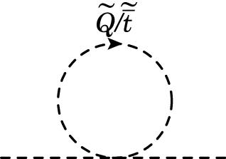
where $\Lambda$ is the ultraviolet momentum cutoff. All diagrams which contain the quadratic divergence are shown in Figure 2.1. If one assume that the standard model is valid up to the Planck scale, the ultraviolet cutoff is naïvely the Planck scale, $\Lambda\sim 10^{19}\,{\rm GeV}$ . Although these radiative corrections can be renormalized by the bare parameter $\mu^{2}_{0}$ , it requires incredible fine-tuning cancellation between the bare mass $\mu^{2}_{0}$ and the quadratic radiative corrections $\Delta\mu^{2}$ . In fact, in order for the $\mathcal{O}(100)\,{\rm GeV}$ electroweak scale to be realized, the $10^{-34}$ fine-tuning is required. This difficulty in the standard model is called the hierarchy problem.

2.2 Supersymmetry and Minimal Model

Refer to caption — Figure 2.1: The quadratic divergence to the mass of the Higgs boson in the standard model and the supersymmetric model. Since the supersymmetry assures that the Higgs quartic coupling is related to the gauge boson coupling like Eq. (2.30), all quadratic divergence are always canceled out in the supersymmetric model.

The supersymmetry (SUSY) is the one of the symmetry which can solve the hierarchy problem. In this section, we first introduce the supersymmetry and its minimal model, and show that the hierarchy problem is solved actually. Next, we briefly review the Lagrangian and the mass of the Higgs boson in the supersymmetric minimal model.

2.2.1 Motivations of Supersymmetry

First, let us briefly introduce the supersymmetry, which can solve the hierarchy problem [3, 4, 5, 6, 7]. The supersymmetry is the extension symmetry of the Poincaré group through the introduction of anticommuting spinor generators $Q_{\alpha},\bar{Q}_{\dot{\alpha}}$ , where $\alpha,~\dot{\alpha}$ are spinor index [28]. It is equal to the symmetry between the boson and fermion,

	$\displaystyle\bar{Q}\|{\rm boson}\rangle$	$\displaystyle=$	$\displaystyle\|{\rm fermion}\rangle$		(2.20)
	$\displaystyle Q\|{\rm fermion}\rangle$	$\displaystyle=$	$\displaystyle\|{\rm boson}\rangle.$		(2.21)

Then, ordinary space-time $x^{\mu}$ is extended to the superspace $(x^{\mu},\theta_{\alpha},\bar{\theta}_{\dot{\alpha}})$ , where $\theta_{\alpha},\bar{\theta}_{\dot{\alpha}}$ are the anticommuting Grassman coordinates. The supersymmetric theories are described by chiral superfield, vector superfield and spinor chiral superfield. The chiral superfield $\hat{\Phi}$ contains the scalar and fermion field on the superspace,

\displaystyle\hat{\Phi}(x,\theta,\bar{\theta})=\phi(y)+\sqrt{2}\theta\psi(y)+\theta\theta F(y),

(2.22)

with $y^{\mu}=x^{\mu}+i\theta\sigma^{\mu}\bar{\theta}$ , and the hat ( $\hat{}$ ) represents the superfield. $\phi$ is a complex scalar field (sfermion), $\psi$ is two-components Weyl spinor field and $F$ is an auxiliary field. The vector superfield $\hat{V}^{a}$ contains the vector boson and fermion field on the superspace,

\displaystyle\hat{V}^{a}(x,\theta,\bar{\theta})=-\theta\sigma^{\mu}\bar{\theta}V^{a}_{\mu}(y)+i\theta\theta\bar{\theta}\bar{\lambda}^{a}(y)-i\bar{\theta}\bar{\theta}\theta\lambda^{a}(y)+\frac{1}{2}\theta\theta\bar{\theta}\bar{\theta}\left(D^{a}(y)-i\partial^{\mu}V^{a}_{\mu}(y)\right),

(2.23)

where $a$ is the index of the generator of the gauge group, $V^{a}_{\mu}$ is the gauge boson, $\lambda_{a}$ is two-components Weyl spinor field (gaugino) and $D_{a}$ is an auxiliary field. The spinor chiral superfield $\hat{W}^{a}_{\alpha}$ also contains the vector boson and fermion field on the superspace,

\displaystyle\hat{W}^{a}_{\alpha}(x,\theta,\bar{\theta})=-i\lambda^{a}_{\alpha}(y)+\left(\delta_{\alpha}^{\beta}D^{a}(y)-\frac{i}{2}(\sigma^{\mu}\bar{\sigma}^{\nu})_{\alpha}^{\beta}V^{a}_{\mu\nu}(y)\right)\theta_{\beta}+\theta\theta\sigma_{\alpha\dot{\alpha}}^{\mu}\partial_{\mu}\bar{\lambda}^{a\dot{\alpha}}(y),

(2.24)

where $V^{a}_{\mu\nu}=\partial_{\mu}V^{a}_{\nu}-\partial_{\nu}V^{a}_{\mu}$ .

The supersymmetric minimal model is called Minimal Supersymmetric Standard Model (MSSM). Table 2.1 shows all chiral and vector superfields with their components for spin $0$ , $1/2$ and $1$ , and their representations for SU $(3)_{c}\times$ SU $(2)_{L}\times$ U $(1)_{Y}$ gauge group in the MSSM. Here the tilde ( $\tilde{}$ ) represents the SUSY partner of the SM particle. Note that, although the number of Higgs doublet is one in the SM, we must introduce two Higgs doublets in the SUSY model,

\displaystyle\hat{H_{1}}=\left(\begin{array}[]{cc}\hat{H_{1}^{0}}\\ \hat{H_{1}^{-}}\end{array}\right),~~~~~~~~\hat{H_{2}}=\left(\begin{array}[]{cc}\hat{H_{2}^{+}}\\ \hat{H_{2}^{0}}\end{array}\right),

where $\tilde{H}$ is called Higgsino. It is because that an existence of the Yukawa interaction with quark/lepton and the gauge anomaly cancelation require two kinds of the Higgs doublets that the hypercharge is opposite.

Table 2.1: All chiral and vector superfields with their components for spin

0

1/2

and

1

, and their representations for SU

(3)_{c}\times

(2)_{L}\times

(1)_{Y}

gauge group in the MSSM.


Chiral Supermultiplet	Spin 0	Spin $\frac{1}{2}$	$SU(3)_{C}$	$SU(2)_{L}$	$U(1)_{Y}$
Quark-Squark $\hat{Q}$	$\tilde{Q}=(\tilde{u}_{L},\tilde{d}_{L})^{T}$	$Q=(u_{L},d_{L})^{T}$	$\bm{3}$	$\bm{2}$	$\frac{1}{6}$
$\hat{\bar{U}}$	$\tilde{\bar{u}}_{R}$	$u_{R}^{\dagger}$	$\bm{3}$	$\bm{1}$	$-\frac{2}{3}$
$\hat{\bar{D}}$	$\tilde{\bar{d}}_{R}$	$d_{R}^{\dagger}$	$\bm{3}$	$\bm{1}$	$\frac{1}{3}$
Lepton-Slepton $\hat{L}$	$\tilde{L}=(\tilde{\nu}_{e},\tilde{e}_{L})^{T}$	$L=(\nu_{e},e_{L})^{T}$	$\bm{1}$	$\bm{2}$	$-\frac{1}{2}$
$\hat{\bar{E}}$	$\tilde{\bar{e}}_{R}$	$e_{R}^{\dagger}$	$\bm{1}$	$\bm{1}$	$1$
Higgs-Higgsino $\hat{H}_{1}$	$H_{1}=(H_{1}^{0},H_{1}^{-})^{T}$	$\tilde{H}_{1}=(\tilde{H}_{1}^{0},\tilde{H}_{1}^{-})^{T}$	$\bm{1}$	$\bm{2}$	$-\frac{1}{2}$
$\hat{H}_{2}$	$H_{2}=(H_{2}^{+},H_{2}^{0})^{T}$	$\tilde{H}_{2}=(\tilde{H}_{2}^{+},\tilde{H}_{2}^{0})^{T}$	$\bm{1}$	$\bm{2}$	$\frac{1}{2}$
Vector Supermultiplet	Spin $\frac{1}{2}$	Spin 1	$SU(3)_{C}$	$SU(2)_{L}$	$U(1)_{Y}$
Gluon-Gluimo $V_{G}$	$\tilde{g}$	$G_{\mu}$	$\bm{8}$	$\bm{1}$	0
W boson-Wino $V_{W}$	$\tilde{W}^{\pm},\ \tilde{W}^{0}$	$W^{\pm}_{\mu},\ W^{0}_{\mu}$	$\bm{1}$	$\bm{3}$	0
B boson-Bino $V_{B}$	$\tilde{B}^{0}$	$B^{0}_{\mu}$	$\bm{1}$	$\bm{1}$	0

As we will discuss in detail later, the Higgs quartic coupling Eq. (2.10) and the gauge coupling are related. In the MSSM, this relation is given as

\displaystyle\lambda_{\rm quartic}=g^{2}(t^{a})^{2}.

(2.30)

Figure 2.1 shows the quadratic divergence to the mass of the Higgs boson in the MSSM. Obviously, the quadratic divergence by the top quark loop Eq. (2.19) is canceled out by the stop loop which are SUSY partners of the top quark. Furthermore, the relationship Eq. (2.30) can cancel out the quadratic divergence by the gauge boson, Higgs boson, gaugino and Higgsino. Actually, all quadratic divergence are always canceled out in the supersymmetric model [6, 7]. Therefore, the supersymmetry can solve the hierarchy problem.

Other motivation of the supersymmetry is dark matter. The SM does not include dark matter, which is stable and does not interact with the electromagnetic force. In the supersymmetric model, in order to forbid all harmful terms, which break baryon number ( $B$ ) and lepton number ( $L$ ) and thus cause the proton decay, one should add a new symmetry. This symmetry is called the $R$ parity [29]. It is defined as

\displaystyle P_{R}=(-1)^{3(B-L)+2s},

(2.31)

where $s$ is the spin and $B=1/3$ for $\hat{Q}$ , $B=-1/3$ for $\hat{\bar{U}},~\hat{\bar{D}}$ , $B=0$ for all others, $L=1$ for $\hat{L}$ , $L=-1$ for $\hat{\bar{E}}$ and $L=0$ for all others. Thus, the SM fermions, Higgs bosons and gauge bosons have even $R$ parity ( $P_{R}=+1$ ), while the squarks, sleptons, Higgsinos and gauginos have odd $R$ parity ( $P_{R}=-1$ ). This symmetry is equal to discrete $\mathbb{Z}_{2}$ R-symmetry. If the $R$ parity is exact symmetry, the lightest supersymmetric particle (LSP) becomes stable. Here the supersymmetric particles are defined as the $R$ parity odd ones. Therefore, when the LSP does not have the electromagnetic charge, it can be a natural candidate of the dark matter.

Another motivation of the supersymmetry is the gauge unification. In fact, the electromagnetic and weak nuclear interactions are unified by the electroweak theory above the unification energy $\mathcal{O}(100)\,{\rm GeV}$ , it is so-called Glashow-Weinberg-Salam theory [19, 20]. In this sense, the electroweak interaction and strong interaction may be unified by grand unification theory (GUT). In fact, although the gauge couplings can not unify in the SM, in the SUSY model the unification of the gauge couplings can occur [30]. Let us briefly observe this fact. The one-loop level renormalization group equations (RGEs) for the gauge couplings in the SM are

\displaystyle\frac{dg^{\prime}}{d{\rm ln}Q}=\frac{1}{(4\pi)^{2}}\frac{41}{6}g^{\prime 3},~~~~~\frac{dg}{d{\rm ln}Q}=-\frac{1}{(4\pi)^{2}}\frac{19}{6}g^{3},~~~~~\frac{dg_{s}}{d{\rm ln}Q}=-\frac{1}{(4\pi)^{2}}7g_{s}^{3},

(2.32)

where $Q$ is the renormalization scale. While, the corresponding equations in the MSSM are

\displaystyle\frac{dg^{\prime}}{d{\rm ln}Q}=\frac{1}{(4\pi)^{2}}11g^{\prime 3},~~~~~\frac{dg}{d{\rm ln}Q}=\frac{1}{(4\pi)^{2}}g^{3},~~~~~\frac{dg_{s}}{d{\rm ln}Q}=-\frac{1}{(4\pi)^{2}}3g_{s}^{3}.

(2.33)

Two-loop level RGEs for all couplings are summarized in Appendix B.1.

Figure 2.2 and 2.3 show the two-loop level running couplings as a function of the renormalization scale $Q$ . In Figure 2.2, the black lines represent $\sqrt{5/3}g^{\prime}(Q)$ ^#1^#1 #1 The factor $\sqrt{5/3}$ is a normalization factor for the GUT., the blue lines represent $g(Q)$ and the red lines represent $g_{s}(Q)$ . In the left panel, the dashed lines correspond the running gauge couplings in the SM, while the solid lines correspond the running gauge couplings in the MSSM with $\,{M_{\rm SUSY}}=10\,{\rm TeV}$ , here $\,{M_{\rm SUSY}}$ represents typical SUSY particles mass scale. As one can see, in the MSSM three gauge couplings are actually unified at GUT sale: $M_{\rm GUT}\simeq 2.0\times 10^{16}\,{\rm GeV}$ , while in the SM it can not achieve. This fact gives one of the main motivations for the SUSY GUT models [31, 32]. In the right panel, we show the running gauge couplings in the MSSM with $\,{M_{\rm SUSY}}=1\,{\rm TeV}$ (upper) and $\,{M_{\rm SUSY}}=100\,{\rm TeV}$ (lower). We find that when $\,{M_{\rm SUSY}}\gtrsim\mathcal{O}(100)\,{\rm TeV}$ , the gauge coupling unification is no longer achieved if one takes universal SUSY particle mass in the MSSM. Thus, this figure implies that when mass scales of all SUSY particles are the same order, the GUT suggests that typical SUSY particles mass scale is $\,{M_{\rm SUSY}}\lesssim\mathcal{O}(100)\,{\rm TeV}$ .

In Figure 2.3, the red lines represent the running top Yukawa coupling $y_{t}(Q)$ , the blue lines represent the running bottom Yukawa coupling $y_{b}(Q)$ , the green lines represent the running tau Yukawa coupling $y_{\tau}(Q)$ and the black lines represent the running Higgs quartic coupling $\lambda_{\rm quartic}(Q)$ . The dashed lines correspond the running couplings in the SM, while the solid lines correspond the running couplings in the MSSM with $\,{M_{\rm SUSY}}=10\,{\rm TeV}$ . We take $\tan\beta=2$ in the left panel, and $\tan\beta=50$ in the right panel. The definition of $\tan\beta$ is given in next section. The important point in these figures is that the Higgs quartic coupling becomes negative at the high energy scale in the SM. If one take $m_{h}\simeq 125\,{\rm GeV}$ , then the Higgs quartic coupling becomes negative at $Q\gtrsim 10^{\rm 10-11}\,{\rm GeV}$ [33]. This situation is avoided in the supersymmetric theory. It is because that the relation between the quartic coupling and the gauge couplings Eq. (2.30) assures the stability of the $\lambda_{\rm quartic}$ .

2.2.2 Lagrangian and the Higgs Boson Mass in the MSSM

Next, we brief review the Lagrangian and the Higgs boson mass of the MSSM [34].

Using the chiral superfield Eq. (2.22), the vector superfield Eq. (2.23) and the spinor chiral superfield Eq. (2.24), the SUSY invariant Lagrangian of the MSSM is given as follows,

\displaystyle\mathcal{L}=\int d\theta^{2}d\bar{\theta}^{2}K\left[\hat{\Phi},\hat{\Phi}^{\dagger},\hat{V}\right]+\left(\int d\theta^{2}W\left[\hat{\Phi}\right]+\rm H.c.\right)+\left(\frac{1}{4}\int d\theta^{2}\hat{W}^{\alpha}\hat{W}_{\alpha}+\rm H.c.\right),

(2.34)

where $K$ is the following Kähler potential

\displaystyle K\left[\hat{\Phi},\hat{\Phi}^{\dagger},\hat{V}\right]=\sum_{\hat{\Phi}}\hat{\Phi}^{\dagger}{\rm Exp}(gt^{a}\hat{V}^{a})\hat{\Phi},

(2.35)

and $W$ is the following superpotential

	$\displaystyle W$	$\displaystyle=$	$\displaystyle\mu\hat{H}_{2}\hat{H}_{1}+W_{\text{Yukawa}},$		(2.36)
	$\displaystyle W_{\text{Yukawa}}$	$\displaystyle=$	$\displaystyle\hat{\bar{U}}\mathbf{y_{u}}\hat{Q}\hat{H_{2}}-\hat{\bar{D}}\mathbf{y_{d}}\hat{Q}\hat{H_{1}}-\hat{\bar{E}}\mathbf{y_{e}}\hat{L}\hat{H_{1}},$		(2.37)

where $\mu$ is the supersymmetric mass of the Higgs multiplets. When the supersymmetry is broken, $\mu$ becomes the mass of the Higgsinos. While the superpotential $W_{\text{Yukawa}}$ gives the supersymmetric Yukawa couplings of the standard model. In fact, the Yukawa matrices $\mathbf{y_{u}},\mathbf{y_{d}}$ and $\mathbf{y_{e}}$ are given approximately as follows

\displaystyle\mathbf{y_{u}}\simeq\begin{pmatrix}0&0&0\\ 0&0&0\\ 0&0&y_{t}\end{pmatrix},~~~\mathbf{y_{d}}\simeq\begin{pmatrix}0&0&0\\ 0&0&0\\ 0&0&y_{b}\end{pmatrix},~~~\mathbf{y_{e}}\simeq\begin{pmatrix}0&0&0\\ 0&0&0\\ 0&0&y_{\tau}\end{pmatrix}.

(2.38)

Here and the following, we use these approximations of Yukawa matrices. Then, the superpotential becomes

$\displaystyle W_{\text{Yukawa}}$	$\displaystyle=$	$\displaystyle y_{t}\hat{\bar{t}}_{R}\hat{Q}\hat{H_{2}}-y_{b}\hat{\bar{b}}_{R}\hat{Q}\hat{H_{1}}-y_{\tau}\hat{\bar{\tau}}_{R}\hat{L}\hat{H_{1}}$	(2.39)
	$\displaystyle=$	$\displaystyle y_{t}(\hat{\bar{t}}_{R}\hat{t}_{L}\hat{H}^{0}_{2}-\hat{\bar{t}}_{R}\hat{b}_{L}\hat{H}^{+}_{2})+y_{b}(\hat{\bar{b}}_{R}\hat{b}_{L}\hat{H}^{0}_{1}-\hat{\bar{b}}_{R}\hat{t}_{L}\hat{H}^{-}_{1})$
		$\displaystyle+y_{\tau}(\hat{\bar{\tau}}_{R}\hat{\tau}_{L}\hat{H}^{0}_{1}-\hat{\bar{\tau}}_{R}\hat{\nu}_{\tau}\hat{H}^{-}_{1}).$

Finally, as the spinor chiral superfields $\hat{W}^{\alpha}$ we take the U(1)_Y gauge multiplets (the B boson and the bino), the SU(2)_L gauge multiplets (the W bosons and the winos) and the SU(3)_c gauge multiplets (the gluons and the gluinos).

Because the supersymmetry is broken in nature, one has to also introduce SUSY breaking terms in Lagrangian. The supersymmetry must be broken softly in order to ensure the cancelation of the quadratic divergences. Generally, the soft SUSY breaking terms are gaugino masses, scalar masse, and trilinear coupling terms for scalars. In the MSSM, the soft SUSY breaking Lagrangian is given as

\displaystyle\mathcal{L}_{\text{soft}}=-V_{\text{soft gaugino}}-V_{\text{soft Yukawa}}-V_{\text{soft Higgs}},

(2.40)

with

$\displaystyle V_{\text{soft gaugino}}$	$\displaystyle=$	$\displaystyle\frac{1}{2}\left(M_{1}\tilde{B}\tilde{B}+M_{2}\tilde{W}\tilde{W}+M_{3}\tilde{g}\tilde{g}\right)+\rm H.c.,$	(2.41)
$\displaystyle V_{\text{soft Yukawa}}$	$\displaystyle=$	$\displaystyle m^{2}_{{Q}}\tilde{Q}^{\dagger}\tilde{Q}+m^{2}_{{{U}}}\tilde{\bar{U}}^{\ast}\tilde{\bar{U}}+m^{2}_{{{D}}}\tilde{\bar{D}}^{\ast}\tilde{\bar{D}}+m^{2}_{{L}}\tilde{L}^{\dagger}\tilde{L}+m^{2}_{{{E}}}\tilde{\bar{E}}^{\ast}\tilde{\bar{E}}$	(2.42)
		$\displaystyle+\left(\tilde{\bar{U}}\mathbf{y_{u}}\mathbf{A_{u}}\tilde{Q}\cdot H_{2}-\tilde{\bar{D}}\mathbf{y_{d}}\mathbf{A_{d}}\tilde{Q}\cdot H_{1}-\tilde{\bar{E}}\mathbf{y_{e}}\mathbf{A_{e}}\tilde{L}\cdot H_{1}+\rm H.c.\right),$	(2.42)
$\displaystyle V_{\text{soft Higgs}}$	$\displaystyle=$	$\displaystyle m_{1}^{2}\|H_{1}\|^{2}+m_{2}^{2}\|H_{2}\|^{2}+\frac{1}{2}(B\mu H_{2}H_{1}+\rm H.c.),$	(2.43)

where $M_{i}$ are the gaugino masses, $m^{2}_{Q/U/D/L/E}$ are the squark/slepton masses, $m^{2}_{1/2}$ are soft SUSY breaking Higgs mass, $A_{i}$ are called $A$ terms and $B$ is called $B$ terms. Note that $m^{2}_{\tilde{i}}$ are flavor generation mixing $3\times 3$ matrix generally. Without additional assumptions, these off-diagonal squark/slepton masses are not suppressed. Adding the soft SUSY breaking Lagrangian Eq. (2.40) into the SUSY invariant Lagrangian Eq. (2.34), one can obtain the full Lagrangian of the MSSM.

Now, let us see the Higgs sector and the mass of the neutral Higgs boron of the MSSM. The tree-level Higgs scalar potential is given directly from Eqs. (2.40, 2.34) as

	$\displaystyle V_{\rm Higgs}$	$\displaystyle=$	$\displaystyle\frac{g^{2}}{2}\left\|H_{1}^{\dagger}H_{2}\right\|^{2}+\frac{g^{2}+g^{\prime 2}}{8}\left(\|H_{1}\|^{2}-\|H_{2}\|^{2}\right)^{2}+\left(\|\mu\|^{2}+m_{1}^{2}\right)\|H_{1}\|^{2}+\left(\|\mu\|^{2}+m_{2}^{2}\right)\|H_{2}\|^{2}$		(2.44)
			$\displaystyle+\frac{1}{2}(B\mu H_{2}H_{1}+\rm H.c.).$		(2.44)

Using the freedom of SU $(2)$ rotations, one can always choose $\langle H_{2}^{+}\rangle=0$ . Then, a potential minimization condition $\partial V/\partial H_{2}^{+}=0$ leads to $\langle H_{1}^{-}\rangle=0$ . Thus, scalar potential of the neutral Higgs boson is given as

	$\displaystyle V_{\rm Higgs}$	$\displaystyle=$	$\displaystyle\frac{g^{2}+g^{\prime 2}}{8}\left(\|H_{1}^{0}\|^{2}-\|H_{2}^{0}\|^{2}\right)^{2}+\left(\|\mu\|^{2}+m_{1}^{2}\right)\|H_{1}^{0}\|^{2}+\left(\|\mu\|^{2}+m_{2}^{2}\right)\|H_{2}^{0}\|^{2}$		(2.45)
			$\displaystyle-\frac{1}{2}\left(B\mu H_{2}^{0}H_{1}^{0}+\rm H.c.\right).$		(2.45)

The potential minimization conditions $\partial V/\partial H_{1}^{0}=0$ and $\partial V/\partial H_{2}^{0}=0$ leads to

	$\displaystyle(m_{1}^{2}+\|\mu\|^{2})v_{1}^{\ast}+\frac{g^{2}+g^{\prime 2}}{4}(\|v_{1}\|^{2}-\|v_{2}\|^{2})v_{1}^{\ast}-\frac{1}{2}B\mu v_{2}$	$\displaystyle=$	$\displaystyle 0,$		(2.46)
	$\displaystyle(m_{2}^{2}+\|\mu\|^{2})v_{2}^{\ast}-\frac{g^{2}+g^{\prime 2}}{4}(\|v_{1}\|^{2}-\|v_{2}\|^{2})v_{2}^{\ast}-\frac{1}{2}B\mu v_{1}$	$\displaystyle=$	$\displaystyle 0,$		(2.47)

where $v_{1/2}$ is the dev of $H_{1/2}^{0}$ . If the determinant of $\partial^{2}V/(\partial H_{i}^{0}\partial H_{j}^{0})$ is negative, one linear combination of $H_{1}^{0}$ and $H_{2}^{0}$ has a negative square mass, then $H_{1}^{0}$ and $H_{2}^{0}$ obtain nonzero vevs. This condition at the vicinity of $H_{1}^{0}=H_{2}^{0}=0$ is

\displaystyle B^{2}\mu^{2}>4(m_{1}^{2}+|\mu|^{2})(m_{2}^{2}+|\mu|^{2}).

(2.48)

In this case, using a redefinition of the phase of $H_{1}^{0}$ and $H_{2}^{0}$ , one can always choose that $B\mu$ , $v_{1}$ and $v_{2}$ are real and positive. Let us defined the ratio of the Higgs vev as

	$\displaystyle\tan\beta$	$\displaystyle\equiv$	$\displaystyle\frac{v_{2}}{v_{1}},$		(2.49)
	$\displaystyle v_{EW}=\sqrt{v_{1}^{2}+v_{2}^{2}}$	$\displaystyle=$	$\displaystyle 174.1\text{ GeV}.$		(2.50)

Then, the potential minimization conditions Eqs. (2.46, 2.47) become

	$\displaystyle m_{1}^{2}$	$\displaystyle=$	$\displaystyle-\|\mu\|^{2}+\frac{1}{2}M_{A}^{2}-\frac{1}{2}\left(M_{A}^{2}+M_{Z}^{2}\right)\cos 2\beta,$		(2.51)
	$\displaystyle m_{2}^{2}$	$\displaystyle=$	$\displaystyle-\|\mu\|^{2}+\frac{1}{2}M_{A}^{2}+\frac{1}{2}\left(M_{A}^{2}+M_{Z}^{2}\right)\cos 2\beta,$		(2.52)

where

\displaystyle M_{A}^{2}=2|\mu|^{2}+m_{1}^{2}+m_{2}^{2}.

(2.53)

The vacuum fluctuations of the Higgs field are defined as

	$\displaystyle H_{1}^{0}$	$\displaystyle=$	$\displaystyle v_{1}+\frac{1}{\sqrt{2}}(H_{1R}+iH_{1I}),$
	$\displaystyle H_{2}^{0}$	$\displaystyle=$	$\displaystyle v_{2}+\frac{1}{\sqrt{2}}(H_{2R}+iH_{2I}).$		(2.54)

Now, one can obtain the following mass matrix for the CP even Higgs bosons,

\displaystyle-\mathcal{L}_{\text{CP-even}}=\frac{1}{2}\begin{pmatrix}H_{1R}H_{2R}\end{pmatrix}\begin{pmatrix}M_{A}^{2}\sin^{2}\beta+M_{Z}^{2}\cos^{2}\beta&-\frac{1}{2}(M_{A}^{2}+M_{Z}^{2})\sin 2\beta\\ -\frac{1}{2}(M_{A}^{2}+M_{Z}^{2})\sin 2\beta&M_{A}^{2}\cos^{2}\beta+M_{Z}^{2}\sin^{2}\beta\end{pmatrix}\begin{pmatrix}H_{1R}\\ H_{2R}\end{pmatrix}.

(2.55)

Diagonalizing this mass matrix, the following mass eigenvalues are given^#2^#2 #2 Similarly to the CP even Higgs boson mass, the tree-level mass of the CP-odd Higgs boson $A$ and charged Higgs boson $H^{\pm}$ are given as $\displaystyle M_{A}^{2}$ $\displaystyle=$ $\displaystyle 2|\mu|^{2}+m_{1}^{2}+m_{2}^{2}=\frac{B\mu}{\sin 2\beta},$ (2.56) $\displaystyle m_{H^{\pm}}^{2}$ $\displaystyle=$ $\displaystyle M_{A}^{2}+M_{W}^{2}.$ (2.57)

	$\displaystyle m_{H}^{2}$	$\displaystyle=$	$\displaystyle\frac{1}{2}\left(M_{A}^{2}+M_{Z}^{2}+\sqrt{(M_{A}^{2}-M_{Z}^{2})^{2}+4M_{A}^{2}M_{Z}^{2}\sin^{2}2\beta}\right),$		(2.58)
	$\displaystyle m_{h}^{2}$	$\displaystyle=$	$\displaystyle\frac{1}{2}\left(M_{A}^{2}+M_{Z}^{2}-\sqrt{(M_{A}^{2}-M_{Z}^{2})^{2}+4M_{A}^{2}M_{Z}^{2}\sin^{2}2\beta}\right),$		(2.59)

here we call a eigenstate, which has the heaviest/lightest mass eigenvalue, $H$ / $h$ . In the decoupling limit $M_{A}^{2}\gg M_{Z}^{2}$ , the eigenstate $h$ becomes the SM Higgs boson perfectly. It is because that the couplings of $h$ with SM particles are equal to the one of the SM Higgs boson with SM particles in this limit. Here and the following, we call this eigenstate $h$ SM-like Higgs boson. Thus, one can recognize Eq. (2.59) as the tree-level mass of the SM-like Higgs boson in the MSSM.

In fact, the tree-level mass of the SM-like Higgs boson Eq. (2.59) has an upper bound,

\displaystyle m_{h}^{2}\leq M_{Z}^{2}\cos^{2}2\beta.

(2.60)

In the SUSY model, in order to cancel out the quadratic divergence in the radiative corrections, the Higgs quartic couplings must be related with the gauge couplings (see Figure 2.1 and Eq. (2.30)). In addition, the Higgs quartic couplings decide the mass of the SM-like Higgs boson (see Eq. (2.17)). These are the reason why there are the upper bound on the Higgs boson mass in the SUSY model. Thus, the SM-like Higgs boson mass must be lighter than the Z boson mass at tree-level in the MSSM. However, this mass bound is too severe to explain an observed SM Higgs boson mass, $m_{h}\simeq 125\,{\rm GeV}$ [1, 2].

Radiative corrections to the Higgs boson mass

On the contrary, in 1990, several groups found that radiative corrections can contribute to the mass of the Higgs boson significantly [35, 36, 37, 38, 39, 40] ^#3^#3 #3 At that time, the Large Electron-Positron Collider (LEP) had not excluded the Higgs boson mass up to the Z boson mass region [41]. . The dominant radiative correction comes from the top/stop loop diagrams, which are depicted in Figure 2.4.

The top/stop one-loop effective potential (the Coleman-Weinberg potential [42]) $V_{\rm CW}^{\rm t}$ is given as,

	$\displaystyle V_{\rm CW}^{\rm t}$	$\displaystyle=$	$\displaystyle\frac{3}{32\pi^{2}}\biggl[m_{\tilde{t}_{1}}^{4}\left(\ln\left(\frac{m_{\tilde{t}_{1}}^{2}}{Q^{2}}\right)-\frac{3}{2}\right)+m_{\tilde{t}_{2}}^{4}\left(\ln\left(\frac{m_{\tilde{t}_{2}}^{2}}{Q^{2}}\right)-\frac{3}{2}\right)$		(2.61)
			$\displaystyle~~~~~~-2m_{t}^{4}\left(\ln\left(\frac{m_{t}^{2}}{Q^{2}}\right)-\frac{3}{2}\right)\biggl]\,,$		(2.61)

where the top quark mass is $m^{2}_{t}=y_{t}^{2}|H_{2}^{0}|^{2}$ and $Q$ is the renormalization scale. The stop masses $m_{\tilde{t}_{1}}$ (lighter) and $m_{\tilde{t}_{2}}$ (heavier) are given as the eigenvalues of the following stop mass matrix,

\displaystyle-\mathcal{L}_{\text{stop~mass}}=\begin{pmatrix}\tilde{t}_{L}^{\ast}\tilde{t}_{R}^{\ast}\end{pmatrix}\begin{pmatrix}M_{\tilde{t}_{11}}^{2}&M_{\tilde{t}_{12}}^{2}\\ M_{\tilde{t}_{21}}^{2}&M_{\tilde{t}_{22}}^{2}\end{pmatrix}\begin{pmatrix}\tilde{t}_{L}\\ \tilde{t}_{R}\end{pmatrix},

(2.62)

with

$\displaystyle M_{\tilde{t}_{11}}^{2}$	$\displaystyle=$	$\displaystyle m_{Q}^{2}+y_{t}^{2}\|H_{2}^{0}\|^{2}+\left(\frac{2}{3}\frac{M_{W}^{2}}{v_{EW}^{2}}-\frac{1}{6}\frac{M_{Z}^{2}}{v_{EW}^{2}}\right)\left(\|H_{1}^{0}\|^{2}-\|H_{2}^{0}\|^{2}\right),$
$\displaystyle M_{\tilde{t}_{22}}^{2}$	$\displaystyle=$	$\displaystyle m_{U}^{2}+y_{t}^{2}\|H_{2}^{0}\|^{2}+\left(-\frac{2}{3}\frac{M_{W}^{2}}{v_{EW}^{2}}+\frac{2}{3}\frac{M_{Z}^{2}}{v_{EW}^{2}}\right)\left(\|H_{1}^{0}\|^{2}-\|H_{2}^{0}\|^{2}\right),$
$\displaystyle M_{\tilde{t}_{12}}^{2}$	$\displaystyle=$	$\displaystyle(M_{\tilde{t}_{12}}^{2})^{\ast}$	(2.63)
	$\displaystyle=$	$\displaystyle y_{t}\left(A_{t}^{\ast}(H_{2}^{0})^{\ast}-\mu H_{1}^{0}\right).$	(2.63)

This effective potential gives the following one-loop corrections to the CP even Higgs mass matrix Eq. (2.55),

$\displaystyle\Delta\mathcal{M}^{2}_{11}$	$\displaystyle=$	$\displaystyle\frac{3}{8\pi^{2}}y_{t}^{4}v_{2}^{2}\mu^{2}R_{t}^{2}(m^{2}_{\tilde{t}_{1}}-m^{2}_{\tilde{t}_{2}})^{2}g(m^{2}_{\tilde{t}_{1}},m^{2}_{\tilde{t}_{2}})$	(2.64)
	$\displaystyle+$	$\displaystyle\frac{3}{16\pi^{2}}y_{t}^{2}A_{t}\mu\tan\beta f(Q^{2},m^{2}_{\tilde{t}_{1}},m^{2}_{\tilde{t}_{2}}),$	(2.64)
$\displaystyle\Delta\mathcal{M}^{2}_{22}$	$\displaystyle=$	$\displaystyle\frac{3}{8\pi^{2}}y_{t}^{4}v_{2}^{2}\biggl(\ln{\frac{m^{2}_{\tilde{t}_{1}}m^{2}_{\tilde{t}_{2}}}{m_{t}^{4}}}+2A_{t}R_{t}\ln{\frac{m^{2}_{\tilde{t}_{1}}}{m^{2}_{\tilde{t}_{2}}}}+A_{t}^{2}R_{t}^{2}(m^{2}_{\tilde{t}_{1}}-m^{2}_{\tilde{t}_{2}})^{2}g(m^{2}_{\tilde{t}_{1}},m^{2}_{\tilde{t}_{2}})\biggl)$	(2.65)
	$\displaystyle+$	$\displaystyle\frac{3}{16\pi^{2}}y_{t}^{2}A_{t}\mu\cot\beta f(Q^{2},m^{2}_{\tilde{t}_{1}},m^{2}_{\tilde{t}_{2}}),$	(2.65)
$\displaystyle\Delta\mathcal{M}^{2}_{12}$	$\displaystyle=$	$\displaystyle-\frac{3}{8\pi^{2}}y_{t}^{4}v_{2}^{2}\mu R_{t}\biggl(\ln{\frac{m^{2}_{\tilde{t}_{1}}}{m^{2}_{\tilde{t}_{2}}}}+A_{t}R_{t}(m^{2}_{\tilde{t}_{1}}-m^{2}_{\tilde{t}_{2}})^{2}g(m^{2}_{\tilde{t}_{1}},m^{2}_{\tilde{t}_{2}})\biggl)$	(2.66)
	$\displaystyle-$	$\displaystyle\frac{3}{16\pi^{2}}y_{t}^{2}A_{t}\mu f(Q^{2},m^{2}_{\tilde{t}_{1}},m^{2}_{\tilde{t}_{2}}),$	(2.66)

with $R_{t}=(A_{t}-\mu\cot\beta)/(m^{2}_{\tilde{t}_{1}}-m^{2}_{\tilde{t}_{2}})$ , here we assume $A_{t}$ and $\mu$ to be real for simplisity. The loop functions $f$ and $g$ are given in Appendix B.3. These corrections give the following upper bound on the SM-like Higgs boson mass,

	$\displaystyle m_{h}^{2}$	$\displaystyle\leq$	$\displaystyle M_{Z}^{2}\cos^{2}2\beta+\frac{3}{8\pi^{2}}y_{t}^{4}v^{2}\sin^{2}\beta\biggl(\ln{\frac{m^{2}_{\tilde{t}_{1}}m^{2}_{\tilde{t}_{2}}}{m_{t}^{4}}}+2\frac{(A_{t}-\mu\cot\beta)^{2}}{m^{2}_{\tilde{t}_{1}}-m^{2}_{\tilde{t}_{2}}}\ln{\frac{m^{2}_{\tilde{t}_{1}}}{m^{2}_{\tilde{t}_{2}}}}$		(2.67)
			$\displaystyle\ \ \ \ \ \ \ \ \ \ \ \ \ \ \ \ \ \ \ \ \ \ \ +\frac{(A_{t}-\mu\cot\beta)^{4}}{(m^{2}_{\tilde{t}_{1}}-m^{2}_{\tilde{t}_{2}})^{2}}\left(2-\frac{m^{2}_{\tilde{t}_{1}}+m^{2}_{\tilde{t}_{2}}}{m^{2}_{\tilde{t}_{1}}-m^{2}_{\tilde{t}_{2}}}\ln{\frac{m^{2}_{\tilde{t}_{1}}}{m^{2}_{\tilde{t}_{2}}}}\right)\biggl).$		(2.67)

If we take the universal soft SUSY breaking stop masses,

\displaystyle m^{2}_{{Q}}=m^{2}_{{{U}}}=m^{2}_{\tilde{q}},

(2.68)

the stop masses are written down easily as follows,

\displaystyle m^{2}_{\tilde{t}_{1/2}}\sim m^{2}_{\tilde{q}}+m_{t}^{2}\mp m_{t}(A_{t}-\mu\cot\beta).

(2.69)

Then, the upper bound Eq. (2.67) becomes

\displaystyle m_{h}^{2}\lesssim M_{Z}^{2}\cos^{2}2\beta+\frac{3}{4\pi^{2}}y_{t}^{4}v^{2}\sin^{2}\beta\biggl(\ln{\frac{m^{2}_{\tilde{q}}}{m_{t}^{2}}}+\frac{(A_{t}-\mu\cot\beta)^{2}}{m^{2}_{\tilde{q}}}-\frac{1}{12}\frac{(A_{t}-\mu\cot\beta)^{4}}{m^{4}_{\tilde{q}}}\biggl).

(2.70)

Therefore, the radiative corrections can give significant contributions to the mass of the SM-like Higgs boson. Note that the logarithmic term is given by the first and second diagram from the left in the Figure 2.4. As one can see, when the stop mass is heavy, this term generates large correction. While, the last two terms are given by the first and second diagram from the right in the Figure 2.4, where the bullet represents the $A_{t}$ term interaction. A notable point is that these contributions are maximized by

\displaystyle A_{t}-\mu\cot\beta=\pm\sqrt{6}m_{\tilde{q}}.

(2.71)

Then these contributions can be comparable to the logarithmic one.

2.3 Current status of the MSSM

In this section, we will review the current situation of the MSSM in terms of an observed $125\,{\rm GeV}$ Higgs boson and the constraints from the flavor violation and CP violation process.

2.3.1 125 GeV

On Wednesday, July 4 2012, the ATLAS and CMS collaborations at the LHC experiment declared astonishing announcements that they had observed a new particle which is consistent with the SM Higgs boson [1, 2]. A mass of the new particle had been around $126\,{\rm GeV}$ . The latest measured value of the Higgs boson mass is

	$\displaystyle m_{h}$	$\displaystyle=$	$\displaystyle 125.36\pm 0.37~({\rm stat.})\pm 0.18~({\rm syst.})\,{\rm GeV}~~~~~({\rm ATLAS})~\textrm{\cite[cite]{[\@@bibref{}{Aad:2014aba}{}{}]}},$		(2.72)
	$\displaystyle m_{h}$	$\displaystyle=$	$\displaystyle 125.03~{}^{+0.26}_{-0.27}~({\rm stat.})~{}^{+0.13}_{-0.15}~({\rm syst.})\,{\rm GeV}~~~~~~~~~({\rm CMS})~\textrm{\cite[cite]{[\@@bibref{}{CMS:2014ega}{}{}]}},$		(2.73)

where correspond to integrated luminosities are ${\rm~4.5~fb}^{-1}{\rm~at~}7{\rm~TeV~and~20.3~fb}^{-1}{\rm~at~8~TeV}$ (ATLAS) and ${\rm~5.1~fb}^{-1}{\rm~at~}7{\rm~TeV~and~19.7~fb}^{-1}{\rm~at~8~TeV}$ (CMS). A naïve average of the ATLAS and CMS results is $125.15\pm 0.25\,{\rm GeV}$ [45].

As we discussed in the previous section, such a Higgs boson mass can not be realized in the tree-level estimation of the MSSM. However, the one-loop radiative corrections can actually raise the mass of the SM-like Higgs boson, and so it can be realized. Therefore, considering the radiative corrections to the Higgs boson mass is important and essential in SUSY models.

Although the one-loop order radiative corrections can contribute significantly to the Higgs boson mass, in fact two-loop order radiative corrections give a negative contribution to the one and it is not a negligible contribution [46, 47, 48, 49, 50, 51]. It is because that the QCD corrections first appear in two-loop order diagrams, and they give opposite contributions to the SM-like Higgs boson (cf. see the last term of second line of the two-loop RGE for $\lambda_{\rm quartic}$ Eq. (B.16)). Therefore, in order to predict a reliable Higgs boson mass in SUSY models, one should take the two-loop order radiative corrections to the Higgs boson mass into account.

It is known that there are three ways to achieve the $125\,{\rm GeV}$ SM-like Higgs boson considering the two-loop order radiative corrections. First way is the heavy stop scenario. When stop masses are about $10\,{\rm TeV}$ , the logarithmic corrections which are generated by the stop loop become an appropriate magnitude. Second way is the large stop mixing scenario, namely the large $A_{t}$ term scenario Eq. (2.71). In this way, even when the stop masses are about $1\,{\rm TeV}$ (and $A_{t}\sim 2.5\,{\rm TeV}$ ), the radiative corrections become an appropriate magnitude [52]. Third way is an extended models of the MSSM [9]. The appropriate extension models which can explain the observed Higgs boson mass are singlet extension models, vector-like matter extended models [53, 54], U $(1)$ gauge extended models [55], etc. In the singlet extension models, an additional $F$ -terms can raise the tree-level mass of the Higgs boson^#4^#4 #4 If the additional CP-even singlet scalar is lighter than the Higgs boson, the singlet-doublet mixing can raise the mass of the Higgs boson [56].. In the vector-like matter extended models, similarly to the stop loop, the vector-like particle loop gives the sizable radiative corrections to the Higgs boson mass. In the U $(1)$ gauge extended models, an additional $D$ -terms can raise the tree-level mass of the Higgs boson. Especially, we will focus on a singlet extension model in this thesis.

In the following two sub sections, we will review the two-loop and higher-loop order analysis of the Higgs boson mass in the MSSM. It is because that we have applied this two-loop order analysis of the Higgs boson mass to a singlet extension model.

2.3.1.1 Two-loop level analysis of the Higgs boson mass

Inclusion of the two-loop level radiative corrections is important and indispensable in the calculation of the mass of the Higgs boson in supersymmetric models. In this section, we first review the two-loop level calculation of the mass of the Higgs boson using the RGE [57, 58, 45]. Then, we will show a behavior of the mass of the Higgs boson as a function of SUSY breaking scale and $\tan\beta$ in the MSSM.

Let us assume $v_{\rm EW}\ll M_{\rm SUSY}$ and $M_{\rm gaugino}\sim\mu\sim\sqrt{m^{2}_{0}}=\mathcal{O}(M_{\rm SUSY})$ for simplicity, where $m^{2}_{0}$ represents dimension two soft SUSY breaking mass term of Higgs and sfermion, namely all the sfermions, heavy Higgs doublet $A$ , Higgsinos and gauginos are integrated out at the scale $\,{M_{\rm SUSY}}$ . This assumption of the mass spectrum represents the effective theory below SUSY breaking scale $M_{\rm SUSY}$ to be the SM. In this section, the SM-like (surviving) Higgs doublet $\Phi_{h}$ and heavy Higgs doublet $\Phi_{H}$ are defined as

\displaystyle\left(\begin{array}[]{cc}\Phi_{h}\\ \Phi_{H}\end{array}\right)=\left(\begin{array}[]{cc}\cos\beta&\sin\beta\\ -\sin\beta&\cos\beta\end{array}\right)\left(\begin{array}[]{cc}-\epsilon H_{d}^{\ast}\\ H_{u}\end{array}\right),

where $\epsilon$ is the antisymmetric tensor $\epsilon_{12}=1$ . In the component representation, this equation is the same as follows,

	$\displaystyle\Phi_{h}$	$\displaystyle=$	$\displaystyle\cos\beta\left(\begin{array}[]{cc}-(H_{1}^{-})^{\ast}\\ (H_{1}^{0})^{\ast}\end{array}\right)+\sin\beta\left(\begin{array}[]{cc}H_{2}^{+}\\ H_{2}^{0}\end{array}\right),$
	$\displaystyle\Phi_{H}$	$\displaystyle=$	$\displaystyle-\sin\beta\left(\begin{array}[]{cc}-(H_{1}^{-})^{\ast}\\ (H_{1}^{0})^{\ast}\end{array}\right)+\cos\beta\left(\begin{array}[]{cc}H_{2}^{+}\\ H_{2}^{0}\end{array}\right).$

The potential of the SM-like Higgs $\Phi_{h}$ below SUSY breaking scale can be given by

\displaystyle V(\Phi_{h})=\frac{\lambda_{\rm quartic}}{2}(\Phi_{h}^{{\dagger}}\Phi_{h}-v_{EW}^{2})^{2}.

(2.91)

This potential becomes as follows when it is expanded by vacuum fluctuation of the Higgs boson, $\Phi_{h}^{0}=v_{EW}+\frac{1}{\sqrt{2}}(h+iG^{0})$ ,

\displaystyle V(h)=2v_{EW}^{2}\lambda_{\rm quartic}\left(\frac{h}{\sqrt{2}}\right)^{2}+2v_{EW}\lambda_{\rm quartic}\left(\frac{h}{\sqrt{2}}\right)^{3}+\frac{\lambda_{\rm quartic}}{2}\left(\frac{h}{\sqrt{2}}\right)^{4}.

(2.92)

Namely the tree-level mass of the SM Higgs scalar $h$ is

\displaystyle m_{h}^{2}=2v_{EW}^{2}\lambda_{\rm quartic}.

(2.93)

In order to derive the physical mass of the SM Higgs scalar $h$ from SUSY breaking scale, we connect the two scale, that is SUSY breaking and electroweak scale, using the two-loop RGE for the Higgs quartic coupling. The full set of two-loop RGEs for the coupling constants of the SM using $\overline{MS}$ regularization are presented in appendix B.1.1. Then, we impose mating conditions of the couplings for the RGE at the SUSY breaking (high) and electroweak (weak) scale. Note that we estimate the mass of the Higgs boson at two-loop level (next-to-leading order), we need to include one-loop threshold corrections in these matching conditions.

Matching at high scale

Because supersymmetry ensures the relationship among the dimensionless coupling constants, the Higgs quartic coupling must satisfy the following matching condition at SUSY breaking scale,

\displaystyle\lambda_{\rm quartic}(\,{M_{\rm SUSY}})=\lambda_{\rm LO}(\,{M_{\rm SUSY}})\equiv\frac{1}{4}\left(g^{2}(\,{M_{\rm SUSY}})+g^{\prime 2}(\,{M_{\rm SUSY}})\right)\cos^{2}2\beta.

(2.94)

Now, in order to accurately calculate the mass of the Higgs boson, we need the matching condition including next-to-leading order corrections. The matching condition including one-loop level threshold corrections is given as follows [57, 45]

\displaystyle\lambda_{\rm quartic}(\,{M_{\rm SUSY}})=\lambda_{\rm LO}(\,{M_{\rm SUSY}})+\frac{1}{(4\pi)^{2}}\lambda_{\rm NLO}(\,{M_{\rm SUSY}}),

(2.95)

where

\displaystyle\lambda_{\rm NLO}=\lambda_{\rm NLO}^{\rm reg}+\lambda_{\rm NLO}^{\phi}+\lambda_{\rm NLO}^{\chi^{1}}+\lambda_{\rm NLO}^{\chi^{2}}.

(2.96)

The First term in the right hand $\lambda_{\rm NLO}^{\rm reg}$ is a convention factor from $\overline{MS}$ to $\overline{DR}$ regularization scheme, which gives a correction to the tree-level relation of Eq. (2.94) even in SUSY limit,

\displaystyle\lambda_{\rm NLO}^{\rm reg}

\displaystyle=

\displaystyle-\left[\frac{1}{4}g^{\prime 4}+\frac{1}{2}g^{\prime 2}g^{2}+(\frac{3}{4}-\frac{\cos^{2}2\beta}{6})g^{4}\right].

(2.97)

The other terms, $\lambda_{\rm NLO}^{\phi},\lambda_{\rm NLO}^{\chi^{1}},\lambda_{\rm NLO}^{\chi^{2}}$ are computed using the $\overline{DR}$ regularization scheme.

The second term $\lambda_{\rm NLO}^{\phi}$ is obtained when one integrate out the heavy Higgs multiplet and sfermion at the matching scale. Neglecting all Yukawa coupling except the top quark $y_{t}$ , this term is given as follows,

$\displaystyle\lambda_{\rm NLO}^{\phi}$	$\displaystyle=$	$\displaystyle 3y_{t}^{2}\left[y_{t}^{2}+\frac{1}{2}(g^{2}-\frac{1}{3}g^{\prime 2})\cos 2\beta\right]\ln\frac{m_{Q}^{2}}{\,{M_{\rm SUSY}}^{2}}+3y_{t}^{2}\left[y_{t}^{2}+\frac{2}{3}g^{\prime 2}\cos 2\beta\right]\ln\frac{m_{U}^{2}}{\,{M_{\rm SUSY}}^{2}}$	(2.98)
		$\displaystyle+3y_{t}^{4}\left[2X_{t}^{2}\tilde{F}(\frac{m_{Q}}{m_{U}})-\frac{X_{t}^{4}}{6}\tilde{G}(\frac{m_{Q}}{m_{U}})\right]+\frac{3}{4}y_{t}^{2}X_{t}^{2}\left[g^{\prime 2}\tilde{H}_{1}(\frac{m_{Q}}{m_{U}}+g^{2}\tilde{H}_{2}(\frac{m_{Q}}{m_{U}}))\right]\cos 2\beta$
		$\displaystyle-\frac{y_{t}^{2}}{4}X_{t}^{2}\cos^{2}2\beta(g^{\prime 2}+g^{2})\tilde{H}(\frac{m_{Q}}{m_{U}})-\frac{3}{16}(g^{\prime 2}+g^{2})\sin^{2}4\beta$
		$\displaystyle+\frac{1}{192}\left[29g^{\prime 4}+42g^{\prime 2}g^{2}+53g^{4}-4\cos 4\beta(g^{\prime 4}+6g^{\prime 2}g^{2}+7g^{4})\right.$
		$\displaystyle\left.-9\cos 8\beta(g^{\prime 2}+g^{2})^{2}\right]\ln\frac{m_{A}^{2}}{\,{M_{\rm SUSY}}^{2}}+\frac{\cos^{2}2\beta}{4}\left[2g^{\prime 4}\ln\frac{m_{E}^{2}}{\,{M_{\rm SUSY}}^{2}}\right.$
		$\displaystyle+\frac{8}{3}g^{\prime 4}\ln\frac{m_{U}^{2}}{\,{M_{\rm SUSY}}^{2}}+\frac{2}{3}g^{\prime 4}\ln\frac{m_{D}^{2}}{\,{M_{\rm SUSY}}^{2}}$
		$\displaystyle\left.+\frac{1}{3}(g^{\prime 4}+9g^{4})\ln\frac{m_{Q}^{2}}{\,{M_{\rm SUSY}}^{2}}+(g^{\prime 4}+g^{4})\ln\frac{m_{L}^{2}}{\,{M_{\rm SUSY}}^{2}}\right],$

where loop functions $\tilde{F},\tilde{G},\tilde{H},\tilde{H}_{1},\tilde{H}_{2}$ are defined in appendix B.3, and they are normalized such that $\tilde{F}(1)=\tilde{G}(1)=\tilde{H}(1)=\tilde{H}_{1}(1)=\tilde{H}_{2}(1)=1$ . The stop mixing parameter $X_{t}$ is defined by

\displaystyle X_{t}=\frac{A_{t}-\mu\cot\beta}{\sqrt{m_{Q}m_{U}}}.

(2.99)

When the all masses of the heavy Higgs multiplet and sfermons are the same as SUSY breaking scale, $\lambda_{\rm NLO}^{\phi}$ becomes as follows

	$\displaystyle\lambda_{\rm NLO}^{\phi}$	$\displaystyle=$	$\displaystyle 6y_{t}^{4}\left[X_{t}^{2}-\frac{X_{t}^{4}}{12}\right]+\frac{y_{t}^{2}}{4}X_{t}^{2}\left(g^{\prime 2}+g^{2}\right)(3-\cos 2\beta)\cos 2\beta$		(2.100)
			$\displaystyle-\frac{3}{16}(g^{\prime 2}+g^{2})\sin^{2}4\beta.$		(2.100)

Here dominant term is the first one, and it reproduces the last two terms of the one-loop corrections Eq. (2.70). As we discussed before, this $y_{t}^{4}$ correction is maximized when $X_{t}\simeq\sqrt{6}$ Eq. (2.71). Therefore, the largest threshold correction comes from the mixing of the stops,

\displaystyle\lambda_{\rm NLO,~max}^{\phi}\simeq 18y_{t}^{4}.

(2.101)

Note that the contribution to the mass of the Higgs boson from this threshold correction (2.101) becomes smaller when SUSY breaking scale is higher. There are two reasons why the contribution becomes small. First, the value of the top Yukawa coupling becomes smaller at high scale by the RGE corrections. Second, the renormalization flow of $\lambda_{\rm quartic}$ has a focusing effect. Namely, in order to obtain the 125 GeV Higgs boson, $\lambda_{\rm quartic}$ of the matching condition should be small when SUSY breaking scale is high. Then the dominant contribution comes from not threshold corrections but RGE corrections from SUSY breaking scale to weak scale.

The third one $\lambda_{\rm NLO}^{\chi^{1}}$ is the modification term to the tree-level relation of Eq. (2.94) through the Higgsino-gaugino loop,

\displaystyle\lambda_{\rm NLO}^{\chi^{1}}=-\frac{1}{6}\cos^{2}2\beta\left[2g^{4}\ln\frac{M_{2}^{2}}{\,{M_{\rm SUSY}}^{2}}+(g^{\prime 4}+g^{4})\ln\frac{\mu^{2}}{\,{M_{\rm SUSY}}^{2}}\right].

(2.102)

The last term $\lambda_{\rm NLO}^{\chi^{2}}$ is obtained as follows when one integrate out the Higgsinos and gauginos at the matching scale,

$\displaystyle\lambda_{\rm NLO}^{\chi^{2}}$	$\displaystyle=$	$\displaystyle\frac{1}{2}\tilde{\beta}_{\lambda}\ln\frac{\mu^{2}}{\,{M_{\rm SUSY}}^{2}}+\left[-\frac{7}{12}\tilde{f}_{1}(r_{1})(\tilde{g}_{1d}^{4}+\tilde{g}_{1u}^{4})-\frac{9}{4}\tilde{f}_{2}(r_{2})(\tilde{g}_{2d}^{4}+\tilde{g}_{2u}^{4})\right.$	(2.103)
		$\displaystyle-\frac{3}{2}\tilde{f}_{3}(r_{1})\tilde{g}_{1d}^{2}\tilde{g}_{1u}^{2}-\frac{7}{2}\tilde{f}_{4}(r_{2})\tilde{g}_{2d}^{2}\tilde{g}_{2u}^{2}-\frac{8}{3}\tilde{f}_{5}(r_{1},r_{2})\tilde{g}_{1d}\tilde{g}_{1u}\tilde{g}_{2d}\tilde{g}_{2u}$
		$\displaystyle-\frac{7}{6}\tilde{f}_{6}(r_{1},r_{2})(\tilde{g}_{1d}^{2}\tilde{g}_{2d}^{2}+\tilde{g}_{1u}^{2}\tilde{g}_{2u}^{2})-\frac{1}{6}\tilde{f}_{7}(r_{1},r_{2})(\tilde{g}_{1d}^{2}\tilde{g}_{2u}^{2}+\tilde{g}_{1u}^{2}\tilde{g}_{2d}^{2})$
		$\displaystyle-\frac{4}{3}\tilde{f}_{8}(r_{1},r_{2})(\tilde{g}_{1d}\tilde{g}_{2u}+\tilde{g}_{1u}\tilde{g}_{2d})(\tilde{g}_{1d}\tilde{g}_{2d}+\tilde{g}_{1u}\tilde{g}_{2u})$
		$\displaystyle+\frac{2}{3}\tilde{f}(r_{1})\tilde{g}_{1d}\tilde{g}_{1u}\left[\lambda_{\rm LO}-2(\tilde{g}_{1d}^{2}+\tilde{g}_{1u}^{2})\right]+2\tilde{f}(r_{2})\tilde{g}_{2d}\tilde{g}_{2u}\left[\lambda_{\rm LO}-2(\tilde{g}_{2d}^{2}+\tilde{g}_{2u}^{2})\right]$
		$\displaystyle\left.+\frac{1}{3}\tilde{g}(r_{1})\lambda_{\rm LO}(\tilde{g}_{1d}^{2}+\tilde{g}_{1u}^{2})+\tilde{g}(r_{2})\lambda_{\rm LO}(\tilde{g}_{2d}^{2}+\tilde{g}_{2u}^{2})\right],$

with

	$\displaystyle\tilde{g}_{1d}$	$\displaystyle=$	$\displaystyle g^{\prime}\sin\beta,~~~~~~\tilde{g}_{2d}=g\sin\beta,$
	$\displaystyle\tilde{g}_{1u}$	$\displaystyle=$	$\displaystyle g^{\prime}\cos\beta,~~~~~~\tilde{g}_{2u}=g\cos\beta,$		(2.104)

	$\displaystyle\tilde{\beta}_{\lambda}$	$\displaystyle=$	$\displaystyle 2\lambda_{\rm LO}(\tilde{g}_{1d}^{2}+\tilde{g}_{1u}^{2}+3\tilde{g}_{2d}^{2}+3\tilde{g}_{2u}^{2})-\tilde{g}_{1d}^{4}-\tilde{g}_{1u}^{4}-5\tilde{g}_{2d}^{4}-5\tilde{g}_{2u}^{4}$		(2.105)
			$\displaystyle-4\tilde{g}_{1d}\tilde{g}_{1u}\tilde{g}_{2d}\tilde{g}_{2u}-2(\tilde{g}_{1d}^{2}+\tilde{g}_{2u}^{2})(\tilde{g}_{1u}^{2}+\tilde{g}_{2d}^{2}),$		(2.105)

and $r_{1}=M_{1}/\mu$ , $r_{2}=M_{2}/\mu$ ^#5^#5 #5 In the split case, $v_{\rm EW}\sim M_{\rm gaugino}\sim\mu\ll M_{\rm SUSY}$ , one must include this threshold correction $\lambda_{\rm NLO}^{\chi^{2}}$ in matching condition at not the high scale but weak scale, as we discuss later.. The loop functions $\tilde{f}_{i},\tilde{f},\tilde{g}$ ( $i=1,2,\dots,8$ ) are defined in appendix B.3, and they are normalized such that $\tilde{f}(1)=\tilde{g}(1)=\tilde{f}_{1/2/3/4}(1)=\tilde{f}_{5/6/7/8}(1,1)=1$ . When the all masses of the Higgsino and gauginos are the same as SUSY breaking scale, $\lambda_{\rm NLO}^{\chi^{2}}$ becomes as follows

	$\displaystyle\lambda_{\rm NLO}^{\chi^{2}}$	$\displaystyle=$	$\displaystyle\frac{1}{8}(1+\sin 2\beta)\left[-\frac{13}{3}g^{\prime 4}-8g^{\prime 2}g^{2}-17g^{4}\right.$		(2.106)
			$\displaystyle\left.+(\frac{1}{3}g^{\prime 2}+g^{2})\left((g^{\prime 2}+g^{2})\cos 4\beta+2(-g^{\prime 2}+g^{2})\sin 2\beta\right)\right].$		(2.106)

Matching at weak scale

In order to calculate the mass of the Higgs boson at the next-to-leading order, we should include the one-loop corrections to the tree-level mass (2.93). The pole mass of the Higgs boson and the top quark are related to $\lambda_{\rm quartic}(Q)$ and $y_{t}(Q)$ at the $\overline{MS}$ scale $Q$ as

	$\displaystyle m^{2}_{h,\textrm{pole}}$	$\displaystyle=$	$\displaystyle 2v_{EW}^{2}(\lambda_{\rm quartic}(Q)+\delta_{\lambda}(Q)),$		(2.107)
	$\displaystyle m_{t,\textrm{pole}}$	$\displaystyle=$	$\displaystyle\frac{y_{t}(Q)v_{EW}}{1+\delta_{t}(Q)},$		(2.108)

Here $\delta_{\lambda}$ is the full one-loop radiative corrections via SM particle loop derived by Sirlin and Zucchini [59]^#6^#6 #6 Recently, the full two-loop corrections to the Higgs quartic coupling are evaluated [60].. $\delta_{t}$ is the three-loop corrections $\mathcal{O}(\alpha_{s}^{3})$ and the full one-loop radiative corrections via the SM particle loop [61, 62].

	$\displaystyle\delta_{\lambda}(Q)$	$\displaystyle=$	$\displaystyle-\frac{\lambda_{\rm quartic}G_{F}M_{Z}^{2}}{8\pi^{2}\sqrt{2}}\left(\xi F_{1}(Q)+F_{0}(Q)+\frac{F_{-1}(Q)}{\xi}\right),$		(2.109)
	$\displaystyle\delta_{t}(Q)$	$\displaystyle=$	$\displaystyle\delta_{t}^{\rm QCD}(Q)+\delta_{t}^{\rm EW}(Q),$		(2.110)

where $G_{F}$ is the Fermi constant from the muon decay, $(\sqrt{2}G_{F})^{-1/2}=246.21971\pm 0.00006\,{\rm GeV}$ , and $\xi=m_{h}^{2}/M_{Z}^{2}$ , $M_{Z}=91.1876\pm 0.0021\,{\rm GeV}$ . The loop function $F_{0},F_{1}$ and $F_{-1}$ are defined in appendix B.3.

We have used the matching condition for the Higgs quartic coupling Eq. (2.107) at $Q=m_{t}$ with

	$\displaystyle m_{t}$	$\displaystyle=$	$\displaystyle(174.34\pm 0.37({\rm stat})\pm 0.52({\rm syst}))\,{\rm GeV}\textrm{\cite[cite]{[\@@bibref{}{Tevatron:2014cka}{}{}]}},$		(2.111)
	$\displaystyle\alpha_{s}(M_{Z})$	$\displaystyle=$	$\displaystyle 0.1184\pm 0.0007\textrm{\cite[cite]{[\@@bibref{}{Bethke:2009jm}{}{}]}}.$		(2.112)

The values of the SM couplings at $Q=m_{t}$ are computed by Ref. [58], using two-loop 5-flavor $\overline{MS}$ RGE (as initial values they use the $\overline{MS}$ mass of the bottom quark $m_{b}(m_{b})=4.18\,{\rm GeV}$ and the pole mass of the tau lepton $m_{\tau}=1.777\,{\rm GeV}$ .). We use these values in matching condition at the weak scale,

\displaystyle g_{s}(Q=m_{t})

\displaystyle=

\displaystyle 1.1666+0.00314\frac{\alpha_{s}(M_{Z})-0.1184}{0.0007}-0.00046(\frac{m_{t}}{\,{\rm GeV}}-173.35),

$\displaystyle g(Q=m_{t})$	$\displaystyle=$	$\displaystyle 0.6483,$	(2.114)
$\displaystyle g^{\prime}(Q=m_{t})$	$\displaystyle=$	$\displaystyle 0.3587,$	(2.115)
$\displaystyle y_{b}(Q=m_{t})$	$\displaystyle=$	$\displaystyle 0.0156,$	(2.116)
$\displaystyle y_{\tau}(Q=m_{t})$	$\displaystyle=$	$\displaystyle 0.0100.$	(2.117)

Then, the numerical values of the next-to-leading order threshold correction Eqs. (2.109, 2.110) are

$\displaystyle\delta_{\lambda}(m_{t})$	$\displaystyle\simeq$	$\displaystyle 0.0075\lambda_{\rm quartic}(m_{t}),$	(2.118)
$\displaystyle\delta_{t}^{\rm QCD}(m_{t})$	$\displaystyle=$	$\displaystyle-\frac{4}{3\pi}\alpha_{s}(m_{t})-0.92\alpha_{s}^{2}(m_{t})-2.64\alpha_{3}^{3}(m_{t}),$	(2.119)
$\displaystyle\delta_{t}(m_{t})$	$\displaystyle=$	$\displaystyle\delta_{t}^{\rm QCD}(m_{t})+\delta_{t}^{\rm EW}(m_{t})\simeq-0.0600+0.0013.$	(2.120)

We have numerically calculated the mass of the Higgs boson at two-loop level, using two-loop SM RGEs (appendix B.1) from SUSY breaking scale to top quark mass scale and including one-loop threshold corrections (Eqs. (3.69, 2.107)). In the Figure 2.5, we show the predicted mass of the Higgs boson as a function of SUSY breaking scale and $\tan\beta$ . The green regions represent the appropriate Higgs mass $125\,{\rm GeV}<m_{h}<126\,{\rm GeV}$ . We take $M_{\rm gaugino}=\mu=\sqrt{m_{0}^{2}}=M_{\rm SUSY}$ for simplicity. The stop mixing parameter is fixed at $A_{t}(\,{M_{\rm SUSY}})=0$ (upper figure), $A_{t}(\,{M_{\rm SUSY}})=\,{M_{\rm SUSY}}$ (middle figure) and $X_{t}(\,{M_{\rm SUSY}})=\sqrt{6}$ (lower figure). Our results are consistent with the Figure 2 in Ref [45].

We find that at large $\tan\beta$ region, an appropriate Higgs mass is achieved when SUSY breaking scale is $\mathcal{O}(10)\,{\rm TeV}$ . On the other hand, at small $\tan\beta$ region, it is achieved when SUSY breaking scale is $\mathcal{O}(10^{\textrm{5-10}})\,{\rm GeV}$ . We also show that the stop mixing contribution Eq. (2.101), that is the dominant threshold correction, is effective at large $\tan\beta$ region. For example, even when the soft SUSY breaking scale is $\mathcal{O}(1)\,{\rm TeV}$ , the maximal stop mixing can raise the Higgs boson mass to be observed value (see the lower figure). However, we discussed before, this contribution is not effective at small $\tan\beta$ and high-scale SUSY breaking region.

Note that in split case, that is $v_{\rm EW}\sim M_{\rm gaugino}\sim\mu\ll M_{\rm SUSY}\sim\sqrt{m_{0}^{2}}$ , Higgsino and gaugino also affect the RGEs of the quartic coupling of the Higgs boson at $v_{\rm EW}<Q<M_{\rm SUSY}$ in addition to the SM particles. In other words, the following terms is still active at $v_{\rm EW}<Q<M_{\rm SUSY}$ ,

\displaystyle\mathcal{L}=-\frac{1}{\sqrt{2}}\Phi_{h}^{T}i\sigma_{2}(-\tilde{g}_{2d}\sigma^{a}\tilde{W}^{a}+\tilde{g}_{1d}\tilde{B})\tilde{H}_{d}-\frac{1}{\sqrt{2}}\Phi_{h}^{{\dagger}}(\tilde{g}_{2u}\sigma^{a}\tilde{W}^{a}+\tilde{g}_{1u}\tilde{B})\tilde{H}_{u}+\rm H.c.,

(2.121)

where $\tilde{g}_{1d/u}$ and $\tilde{g}_{2d/u}$ are Yukawa-like gaugino couplings. Then, since supersymmetry is no longer ensued at $Q<M_{\rm SUSY}$ , the Yukawa-like gaugino couplings are different from the corresponding gauge couplings^#7^#7 #7 We have also considered the corrections to the gaugino couplings from the corresponding gauge couplings [65, 66] in the split mass spectrum case, in which sleptons are also light. We found that this corrections can be as large as $\sim 10\%$ in the parameter region in which the muon $g-2$ anomaly can be solved, and that the gaugino couplings can be measured from the production cross section of the right-handed selectrons at $1\%$ accuracy at ILC with $\sqrt{s}=500\,{\rm GeV}$ .. Namely, the relations Eq. (2.104) are not satisfied at $Q<M_{\rm SUSY}$ . Therefore, in the split case, we should take into account the RGE of not only the SM couplings but also the Yukawa-like gaugino couplings at $v_{EW}<Q<M_{\rm SUSY}$ . The study of the split mass spectrum case is written in Refs. [57, 45] in detail.

2.3.1.2 Higher-loop radiative corrections to the Higgs boson mass

Recently, the contributions of higher-loop correction to the mass of the Higgs mass have been studied. As a result, one find that these new contributions are important when SUSY breaking scale is not low. In this section, we briefly review the higher-loop corrections.

Figure 2.6 shows the mass of the Higgs boson as a function of SUSY breaking scale including the higher-loop radiative corrections. We have numerically analyzed the mass of the Higgs boson using the public code FeynHiggs2.10.0 [67, 68, 69, 70, 71, 72, 73, 74]. We take $m_{Q}=m_{U}=M_{3}=\mu=M_{A}=M_{\rm SUSY}$ , $\tan\beta=50$ and $A_{t}=0$ . In this analysis, the mass of the top quark is $174.34\,{\rm GeV}$ [63], which is the latest result. The green region is $125\,{\rm GeV}<m_{h}<126\,{\rm GeV}$ . The dotted line represents the full one-loop result and the dashed line represents leading $\mathcal{O}(y_{t}^{2}g_{s}^{2})$ plus subleading $\mathcal{O}(y_{t}^{4})$ two-loop result. Note that full one-loop, leading two-loop and subleading two-loop corrections are calculated by Feynman-diagrammatic approach, and these contributions include not only the logarithmic corrections but also finite corrections. The thick line represents the result of two-loop plus higher-loop corrections, which is evaluated by a resummation of the leading and subleasing logarithmic corrections from the scalar top sector. The resummation have been obtained from an analysis of the RGE at two-loop level. The blue and red regions represent one sigma bands from the theoretical uncertainty. The theoretical uncertainty is dominated by two contribution, the experimental error on the mass of the top quark and unknown higher-order corrections. The theoretical uncertainty from the experimental error on the mass of top quark is numerically estimated [75], and it is obtained as follows,

\displaystyle\delta m_{h}^{m_{t}}\sim\delta m_{t}^{\rm exp}\sim 1\,{\rm GeV}.

(2.122)

On the other hand, the theoretical uncertainty from the unknown higher-order corrections is estimated at $\delta m_{h}^{\rm higher}\sim 3$ - $5\,{\rm GeV}$ in two-loop level calculations. However, as you can see Figure 2.6, including the resummation of the leading and subleading logarithmic corrections, this uncertainty dramatically decrease [74, 76] at

\displaystyle\delta m_{h}^{\rm higher}\lesssim 1\,{\rm GeV}.

(2.123)

In this Figure, we show that the higher-order corrections by the resummation of the leading and subleading logarithmic corrections can raise the mass of the Higgs boson. We also find that when there is no help of $A_{t}$ term, SUSY breaking scale is predicted $M_{\rm SUSY}\sim 5\,{\rm TeV}$ in order to obtain an appropriate mass of the Higgs boson ( $\tan\beta=50$ case).

2.3.2 SUSY FCNC / CP Problem

In general, the supersymmetry introduces the new flavor and CP violating sources through the SUSY breaking sector. These new contributions seem to cause the flavor changing neutral currents (FCNC) and electric dipole mordents (EDM) of quarks and leptons. On the other hand, in the SM, the FCNC is suppressed by the GIM mechanism [77], and the EDM is suppressed by the three (four) loop suppression and by the smallness of component of the CP violating phase in the CKM matrix. Hence, the FCNC and EDM which are generated from the SUSY breaking sector can give dominant contributions, and they can be probed by the low energy flavor experiments and the EDM measurements. Nevertheless, the corresponding signals have not been observed yet. The current experimental results set the constraint to the new flavor and CP violating sources in the supersymmetric models.

In the MSSM, the new flavor violations are generated by the off-diagonal sfermion soft SUSY breaking terms $(m^{2}_{\tilde{f}})_{ij}~(i\neq j)$ and the off-diagonal $A$ terms $A_{ij}~(i\neq j)$ . If the $A$ terms are proportional to the Yukawa matrix, the main sources of the flavor violation are given by the sfermion masses. Besides these off-diagonal components are expected the same order as the diagonal components if there are no additional symmetries^#8^#8 #8 The large off-diagonal components cause the negative eigenvalue of sfermion mass square, which leads to the charged/colored breaking vacuum. Thus, actually the off-diagonal components are expected $\mathcal{O}(0.1\times(m^{2}_{\tilde{f}})_{ii})$ .. Thus, the supersymmetry would cause relatively large FCNC process.

One of the severe constraints comes from the branching ratio of $\mu\to e\gamma$ . In the MSSM, when we assume $(m^{2}_{\tilde{\ell}_{L}})_{ij}=(m^{2}_{\tilde{\ell}_{R}})_{ij}=(m^{2}_{\tilde{\nu}})_{ij}$ and neglect the $A$ term contributions, the branching ratio of $\mu\to e\gamma$ at the one-loop order is given as [65, 78],

$\displaystyle\textrm{Br}(\mu\to e\gamma)$	$\displaystyle\simeq$	$\displaystyle\frac{1}{\Gamma_{\rm tot}}\frac{\alpha m_{\mu}}{16}\biggl\|\frac{(m^{2}_{\tilde{\ell}})_{23}(m^{2}_{\tilde{\ell}})_{31}}{m^{4}_{\tilde{\mu}}}\frac{m_{\tau}}{m_{\mu}}a_{\mu,~\textrm{bino(neutralino)~loop}}$	(2.124)
		$\displaystyle~~~~~~~~~~~~~+\frac{(m^{2}_{\tilde{\ell}})_{21}}{m^{2}_{\tilde{\mu}}}\biggl(a_{\mu,~\textrm{chargino~loop}}+a_{\mu,~\textrm{wino-Higgsino(neutralino)~loop}}$
		$\displaystyle~~~~~~~~~~~~~~~~~~~~~~~~~~~~+a_{\mu,~\textrm{bino-Higgsino(neutralino)~loop}}\biggl)\biggl\|^{2},$

with

$\displaystyle a_{\mu,~\textrm{chargino~loop}}$	$\displaystyle=$	$\displaystyle\frac{g^{2}}{16\pi^{2}}\frac{m_{\mu}^{2}}{M_{2}\mu}\tan\beta f_{C}\left(\frac{M_{2}^{2}}{m_{\tilde{\nu}_{2}}^{2}},\frac{\mu^{2}}{m_{\tilde{\nu}_{2}}^{2}}\right),$	(2.125)
$\displaystyle a_{\mu,~\textrm{wino-Higgsino(neutralino)~loop}}$	$\displaystyle=$	$\displaystyle-\frac{g^{2}}{32\pi^{2}}\frac{m_{\mu}^{2}}{M_{2}\mu}\tan\beta f_{N}\left(\frac{M_{2}^{2}}{m_{\tilde{\mu}}^{2}},\frac{\mu^{2}}{m_{\tilde{\mu}}^{2}}\right),$	(2.126)
$\displaystyle a_{\mu,~\textrm{bino-Higgsino(neutralino)~loop}}$	$\displaystyle=$	$\displaystyle-\frac{g^{\prime 2}}{32\pi^{2}}\frac{m_{\mu}^{2}}{M_{1}\mu}\tan\beta f_{N}\left(\frac{M_{1}^{2}}{m^{2}_{\tilde{\mu}}},\frac{\mu^{2}}{m^{2}_{\tilde{\mu}}}\right),$	(2.127)
$\displaystyle a_{\mu,~\textrm{bino(neutralino)~loop}}$	$\displaystyle=$	$\displaystyle\frac{g^{\prime 2}}{16\pi^{2}}\frac{m_{\mu}^{2}M_{1}\mu}{m_{\tilde{\mu}}^{4}}\tan\beta f_{N}\left(\frac{m_{\tilde{\mu}}^{2}}{M_{1}^{2}},\frac{m_{\tilde{\mu}}^{2}}{M_{1}^{2}}\right),$	(2.128)

where $(m^{2}_{\tilde{\ell}_{L}})_{22}\equiv m^{2}_{\tilde{\mu}}$ , the total decay width of muon $\Gamma_{\rm tot}=2.99\times 10^{-19}\,{\rm GeV}$ , and the loop functions $f_{C}$ and $f_{N}$ are defined in Appendix B.3. Note that the SUSY contributions are given by the chargino-sneutrino loop and the neutralino-smuon loop. As one can see, these effects are proportional to $\tan^{2}\beta$ . Naturally, these SUSY contributions are decoupled in the $\,{M_{\rm SUSY}}\to\infty$ .

The current bound on the $\mu\to e\gamma$ had been given by MEG Collaboration, and the result is Br( $\mu\to e\gamma)<5.7\times 10^{-13}~(90~\%$ CL) [79]. The Ref. [80] showed that when $\sqrt{m^{2}_{\tilde{\mu}}}=\mu=\,{M_{\rm SUSY}}$ , $3M_{1}/(5g^{\prime 2})=M_{2}/g^{2}=\,{M_{\rm SUSY}}/g_{s}^{2}$ , $\tan\beta=50$ , $(m^{2}_{\tilde{\ell}})_{21}/m^{2}_{\tilde{\mu}}=0.1$ and $(m^{2}_{\tilde{\ell}})_{23}/m^{2}_{\tilde{\mu}}=(m^{2}_{\tilde{\ell}})_{31}/m^{2}_{\tilde{\mu}}=0$ are taken, the current bound implies that the soft SUSY breaking scale should be heavier than $30\,{\rm TeV}$ , $\,{M_{\rm SUSY}}\gtrsim 30\,{\rm TeV}$ . Thus, this bound severely constrains the low scale SUSY models if there are no additional symmetries or mechanisms. Note that this bound can be relaxed if we take small $\tan\beta$ .

One the other hand, in the MSSM the new CP violation sources are the off-diagonal sfermion soft SUSY breaking masses Im( $(m^{2}_{\tilde{f}})_{ij}$ ) $~(i\neq j)$ , $A$ terms Im( $A_{ij}$ ), the gaugino mass Im( $M_{\rm gaugino}$ ) and the Higgsino mass Im( $\mu$ ). The physical CP violation source is relative phases of those. Although the quark (lepton) EDM is generated by three (four) loop diagram in the SM, the EDM is actually generated by one loop diagram in the SUSY models. Therefore, the supersymmetry also would cause relatively large EDM.

One of the severe constraints to the CP violation phenomena comes from the electron EDM. In the MSSM, when we take the same assumption as the above, the electron EDM at the one-loop order is given as [65],

	$\displaystyle\frac{d_{e}}{e}$	$\displaystyle\simeq$	$\displaystyle-\frac{1}{2m_{e}}\biggl[\textrm{arg}[M_{2}\mu]\left(a_{e,~\textrm{chargino~loop}}+a_{e,~\textrm{wino-Higgsino(neutralino)~loop}}\right)$		(2.129)
			$\displaystyle~~~~~~~+\textrm{arg}[M_{1}\mu]\left(a_{e,~\textrm{bino-Higgsino(neutralino)~loop}}+a_{e,~\textrm{bino(neutralino)~loop}}\right)\biggl],$		(2.129)

where we have replaced subscript $\mu$ with $e$ in the Eqs. (2.125-2.128). Similarly to the $\mu\to e\gamma$ process, the SUSY contributions are given by the chargino-sneutrino loop and the neutralino-smuon loop. These contributions are proportional to the CP violating relative phase of the Higgsino and the gaugino masses and proportional to $\tan\beta$ . When the all dimensional parameter are the same values $M_{1}=M_{2}=\mu=\sqrt{m^{2}_{\tilde{\nu}_{1}}}=\sqrt{m^{2}_{\tilde{e}}}=\,{M_{\rm SUSY}}$ , and if we take the universal CP violating phase of gaugino mass $\textrm{arg}(M_{1}\mu)=\textrm{arg}(M_{2}\mu)=\sin\phi$ , the one loop order electron EDM is given as,

	$\displaystyle\|d_{e}\|$	$\displaystyle\simeq$	$\displaystyle\frac{5g^{2}+g^{\prime 2}}{2\cdot 48\pi\cdot 4\pi}\frac{m_{e}}{\,{M_{\rm SUSY}}^{2}}\tan\beta\sin\phi\times 197\times 10^{-16}~~[e\textrm{~cm}],$		(2.130)
		$\displaystyle=$	$\displaystyle 2.9\times 10^{-27}\left(\frac{10\,{\rm TeV}}{\,{M_{\rm SUSY}}}\right)^{2}\left(\frac{\tan\beta}{50}\right)\sin\phi~~[e\textrm{~cm}].$		(2.130)

The current bound on the electron EDM had been given by ACME Collaboration, and the result is $|d_{e}|<8.7\times 10^{-29}$ [ $e$ cm] $(90~\%$ CL) [81]. The Ref. [80] showed that when $\sqrt{m^{2}_{\tilde{e}}}=\mu=\,{M_{\rm SUSY}}$ , $3M_{1}/(5g^{\prime 2})=M_{2}/g^{2}=\,{M_{\rm SUSY}}/g_{s}^{2}$ , $\tan\beta=50$ , $(m^{2}_{\tilde{\ell}})_{ij}/m^{2}_{\tilde{e}}=0~(i\neq j)$ and the maximal CP violating phase are taken, the current bound implies that the soft SUSY breaking scale should be heavier than $100\,{\rm TeV}$ , $\,{M_{\rm SUSY}}\gtrsim 100\,{\rm TeV}$ . Although this bound can be relaxed if one takes small $\tan\beta$ , it also severely constrains the low scale SUSY models.

Another severe constraint comes from measurement of the CP violation in the kaon decay [82]. Under the CP transformation a neutral kaon $K^{0}~(d\bar{s})$ becomes an anti-neutral kaon $\bar{K}^{0}~(s\bar{d})$ , and it is represented by convention,

	$\displaystyle\bm{{\rm CP}}\|K^{0}\rangle=+\|\bar{K}^{0}\rangle,$
	$\displaystyle\bm{{\rm CP}}\|\bar{K}^{0}\rangle=+\|K^{0}\rangle.$		(2.131)

Hence, $(|K^{0}\rangle+|\bar{K}^{0}\rangle)/\sqrt{2}$ and $(|K^{0}\rangle-|\bar{K}^{0}\rangle)/\sqrt{2}$ states are the CP even and odd eigenstates. Since the CP symmetry is slightly broken in nature, the mass eigenstates of the neutral kaons become the following forms,

	$\displaystyle\|K^{0}_{S}\rangle$	$\displaystyle=$	$\displaystyle\frac{1}{\sqrt{2}}\left[e^{-i\phi_{K}}(1+\epsilon_{K})\|K^{0}\rangle+e^{i\phi_{K}}(1-\epsilon_{K})\|\bar{K}^{0}\rangle\right],$
	$\displaystyle\|K^{0}_{L}\rangle$	$\displaystyle=$	$\displaystyle\frac{1}{\sqrt{2}}\left[e^{-i\phi_{K}}(1+\epsilon_{K})\|K^{0}\rangle-e^{i\phi_{K}}(1-\epsilon_{K})\|\bar{K}^{0}\rangle\right],$		(2.132)

where $\epsilon_{K}$ is an indirect CP violation parameter (CP violation in $K^{0}$ - $\bar{K}^{0}$ mixing) and $\phi_{K}$ is a direct CP violation parameter (CP violation in the neutral kaon decay), and actually $\epsilon_{K}\ll 1,~\phi_{K}\ll 1$ . The indirect CP violation parameter $\epsilon_{K}$ is determined by an imaginary part of the $K^{0}$ - $\bar{K}^{0}$ mixing [83, 84],

\displaystyle\epsilon_{K}=e^{i\phi_{\epsilon}}\sin\phi_{\epsilon}\left(-\frac{\textrm{Im}(\mathcal{M}_{K^{0}\textrm{-}\bar{K}^{0}})}{\Delta M_{K}}+\phi_{K,0}\right),

(2.133)

with

	$\displaystyle\mathcal{M}_{K^{0}\textrm{-}\bar{K}^{0}}$	$\displaystyle=$	$\displaystyle\langle K^{0}\|\mathcal{H}_{\rm eff}^{4fermi}(\bar{d}s\bar{d}s)\|\bar{K}^{0}\rangle,$
	$\displaystyle\tan\phi_{\epsilon}$	$\displaystyle=$	$\displaystyle\frac{2\Delta M_{K}}{\Delta\Gamma_{K}}=(43.52\pm 0.05)^{\circ},$		(2.134)

where $\phi_{K,0}$ is the phase of the 0-isospin amplitude in kaon decay $K^{0}\to 2\pi$ , and

	$\displaystyle\Delta M_{K}$	$\displaystyle=$	$\displaystyle M_{L}-M_{S}=(3.484\pm 0.006)\times 10^{-12}~\,{\rm MeV},$
	$\displaystyle\Delta\Gamma_{K}$	$\displaystyle=$	$\displaystyle\Gamma_{S}-\Gamma_{L}=(7.2823\pm 0.0098)\times 10^{-12}~\,{\rm MeV}.$		(2.135)

The second term of the Eq. (2.133) contributes an $\mathcal{O}$ (5%) correction to $\epsilon_{K}$ [84].

In the SM, the leading contribution of the four-fermion Hamiltonian $\mathcal{H}_{\rm eff}^{4fermi}(\bar{d}s\bar{d}s)$ comes from one-loop box diagrams with the weak interactions and the imaginary component of the CKM matrix. While in the MSSM, the leading SUSY contribution comes from one-loop gluino-squark box diagrams with the strong interaction, and these contributions are easy to affect estimation of $\epsilon_{K}$ . The main CP-violating source of this diagram is the off-diagonal sfermion soft SUSY breaking masses Im $[(m^{2}_{\tilde{d}_{L}})_{12}(m^{2}_{\tilde{d}_{R}})_{12}]$ . The detailed formulae of the SUSY contributions to $\epsilon_{K}$ are given in Ref. [85].

The latest experimental value is $|\epsilon_{K}^{\rm(exp)}|=(2.228\pm 0.011)\times 10^{-3}$ [86] and the SM prediction (including next-to-next-to-leading-order) is $|\epsilon_{K}^{\rm(SM)}|=(1.81\pm 0.28)\times 10^{-3}$ [87]. These numerical values set a conservative upper bound of the SUSY contributions, $|\epsilon_{K}^{\rm(SUSY)}|<0.98\times 10^{-3}$ [80]. The Ref. [80] showed that when $\sqrt{m^{2}_{\tilde{d}}}=M_{3}=\,{M_{\rm SUSY}}$ , $|(m^{2}_{\tilde{d}_{L}})_{ij}/m^{2}_{\tilde{d}}|=|(m^{2}_{\tilde{d}_{R}})_{ij}/m^{2}_{\tilde{d}}|=0.1~(i\neq j)$ and the maximal CP violating phase are taken, the current bound implies that the soft SUSY breaking scale should be heavier than $500\,{\rm TeV}$ , $\,{M_{\rm SUSY}}\gtrsim 500\,{\rm TeV}$ . If one imposes the SO(10) relation at the GUT scale; $(m^{2}_{\tilde{d}_{R}})_{ij}=(m^{2}_{\tilde{d}_{L}})^{\ast}_{ij}$ , the imaginary components of the soft SUSY breaking squark masses vanish at the GUT scale and they are generated only through the RG effects, and thus $\epsilon_{K}^{\rm(SUSY)}$ is suppressed. Then, the current bound implies $\,{M_{\rm SUSY}}\gtrsim 40\,{\rm TeV}$ .

Therefore, when the soft SUSY breaking scale is low scale which is favored in terms of the naturalness, too large FCNC and too large CP-violation are induced by the SUSY particles one-loop radiative corrections. These difficulties are called “the SUSY FCNC problem” and “the SUSY CP problem”.

2.4 Discussions

In previous section, we have reviewed the current situation of the MSSM in terms of an observed 125 GeV Higgs boson and the constraints from the flavor violation and CP violation process. Actually, we have shown the following two points in the MSSM,

•

In order to realize the observed Higgs boson mass, the masses of the stops have to be heavier than 5 TeV or the stop mixing has to be maximized (or their compromised parameter region).
•

In order to avoid the severe constraints from the flavor violation and CP violation measurements, the masses of the sleptons should be heavy and the parameter $\tan\beta$ should be not so large if there are no additional symmetries or mechanisms.

Therefore, in this chapter we naïvely conclude that one of the suitable solutions is the high-scale supersymmetry, which has $\mathcal{O}$ (10-100) TeV soft SUSY breaking terms.

Once we give up thought on the naturalness, such a high-scale supersymmetric model is very attractive. First, as we discussed, the observed 125 GeV Higgs boson and the explanation of the current bound on the flavor violation and CP violation process are simultaneous realized naturally. Second, all the SUSY particles are out of the reach of the current LHC, thus it can explain that there are no signals of the SUSY particles at the LHC experiments. Third, it can naturally solve the cosmological gravitino problem [88]: although an unstable gravitino spoils the big-bang nucleosynthesis, the heavy gravitino (typically heavier than $5$ - $8$ TeV) can avoid the disaster^#9^#9 #9 Here, we implicitly assumed that the soft SUSY breaking scale and the gravitino mass are the same scale.. Fourth, this heavy SUSY breaking scale remains the gauge couplings unification at the GUT scale (see Figure 2.2).

Furthermore, the future prospects of the flavor violation and the CP violation measurements have the potential to probe the supersymmetry beyond the reach of the LHC by orders of magnitude [89, 90, 91, 92, 93, 94, 95, 96]. Therefore, we hope that these precision measurements can indirectly probe the high-scale supersymmetry.

Chapter 3 Singlet Extension

In this chapter, in order to solve the $\mu$ problem of the supersymmetric minimal model, we first introduce a gauge singlet superfield and singlet extension supersymmetric minimal model. Then, we should impose extra symmetries to forbid unwanted terms of singlet superfield, which spoil the solution of the $\mu$ problem. In general, these symmetries lead to the domain wall problem and the tadpole problem. The nearly minimal supersymmetric standard model is the one of the models which can solve the $\mu$ problem, the domain wall problem and the tadpole problem simultaneously. Finally, we review the Lagrangian and the Higgs sector of the nearly minimal supersymmetric standard model, and we show that there is a sizable tree-level contribution to the Higgs boson mass due to an extra F-term contribution to the Higgs quartic coupling.

3.1 $\mu$ Problem

In the MSSM, the potential minimization conditions Eqs. (2.51, 2.52) lead to the following relationship,

\displaystyle M_{Z}^{2}

\displaystyle=

\displaystyle\frac{m_{2}^{2}-m_{1}^{2}}{\cos 2\beta}-M_{A}^{2}=\frac{m_{2}^{2}-m_{1}^{2}}{\cos 2\beta}-m_{1}^{2}-m_{2}^{2}-2|\mu|^{2},

(3.1)

where $\mu$ is the supersymmetric mass of the Higgs multiplets. Especially, when $\tan\beta\gg 1$ , this equation can be expanded by $\tan\beta$ and becomes

\displaystyle M_{Z}^{2}=-2(m_{2}^{2}+|\mu|^{2})+\frac{2}{\tan^{2}\beta}(m_{1}^{2}-m_{2}^{2})+\mathcal{O}(\frac{1}{\tan^{4}\beta}).

(3.2)

These relationships imply that since actually $M_{Z}\sim\mathcal{O}(100)\,{\rm GeV}$ (electroweak scale), $\sqrt{m_{1}^{2}},~\sqrt{m_{2}^{2}}$ and $\mu$ should be naïvely at the electroweak scale, or $\sqrt{m_{1}^{2}},~\sqrt{m_{2}^{2}}$ and $\mu$ should be the same scale to able to cancel out. In other words, the magnitude of $\mu$ have to be the soft SUSY breaking scale $\,{M_{\rm SUSY}}$ or be less than the scale.

One the other hand, the $\mu$ term is stable under the all orders in perturbation theory of the effective Lagrangian due to the non-renormalization theorem [97], and the supersymmetry provides a valid description that the scale of the $\mu$ parameter is as large as GUT scale or Planck scale^#1^#1 #1 Another elegant possibility is $\mu=0$ , which is respected the some symmetries (e.g. Peccei-Quinn symmetry). However, nature have not chosen this values. It is because that the lightest chargino search by the LEP set lower bound on chargino mass, $|\mu|>103.5\,{\rm GeV}$ [98]. . If $\mu$ is at the Planck scale, it leads to $M_{Z}\sim M_{\rm Pl}$ (see Eq. (3.1)), and the appropriate electroweak symmetry breaking can not occur. Therefore, $\mu$ has to know the soft SUSY breaking scale in order to realize the nature, namely the $Z$ boson mass is the electroweak scale. This problem is called “ $\mu$ problem” [8]:

	$\displaystyle\textrm{Why }~\mu\ll M_{\rm GUT},~M_{\rm Pl}~\textrm{?}$
	$\displaystyle\textrm{Why does}~\mu~\textrm{know}~\,{M_{\rm SUSY}}~\textrm{?}$		(3.3)

Table 3.1: The singlet superfield with their components for spin

0

and

1/2

, and their representations for SU

(3)_{c}\times

(2)_{L}\times

(1)_{Y}

gauge group.


Chiral Supermultiplet	Spin 0	Spin $\frac{1}{2}$	$SU(3)_{C}$	$SU(2)_{L}$	$U(1)_{Y}$
Singlet scalars-Singlino $\hat{S}$	$S=(S_{R}+iS_{I})/\sqrt{2}$	$\tilde{S}$	$\bm{1}$	$\bm{1}$	$0$

One of the natural solutions of the $\mu$ problem is the singlet extension models of the MSSM [9]. These models have the following superpotential,

\displaystyle W=\lambda\hat{S}\hat{H}_{2}\hat{H}_{1}+f[\hat{S}]+W_{\rm Yukawa},

(3.4)

where $\hat{S}$ is an additional gauge singlet superfield, $\lambda$ is a dimensionless coupling constant, and $f[\hat{S}]$ is the superpotential which does not depend on superfields of the MSSM at the renormalizable level. The singlet superfield $\hat{S}$ with their components for spin $0$ and $1/2$ are shown in Table 3.1. When supersymmetry is broken, singlet superfiled also receives the soft SUSY breaking mass or $A$ term. At this time, singlet scalar boson can naturally obtain a vev which is the order of the soft SUSY breaking scale, $\langle S\rangle\sim\mathcal{O}(\,{M_{\rm SUSY}})$ , and so its vev gives the effective $\mu$ term for Higgs multiplets,

\displaystyle\mu_{\rm eff}=\lambda\langle S\rangle.

(3.5)

Therefore, the $\mu$ problem can be solved by the singlet extension models of the MSSM ^#2^#2 #2 One of the other solutions of the $\mu$ problem is provided by the Giudice and Masiero [99]. Let us consider the following Kähler potential, $\displaystyle K=c_{1}\frac{1}{M_{\rm Pl}}\hat{X}^{{\dagger}}\hat{H}_{2}\hat{H}_{1}+c_{2}\hat{H}_{2}\hat{H}_{1}+\rm H.c.,$ (3.6) where $c_{1}$ and $c_{2}$ are $\mathcal{O}(1)$ couplings and $\hat{X}$ is an additional gauge singlet superfield. Note that the second term is permitted in the supergravity theory. This Kähler potential can be rewritten to the following superpotential, $\displaystyle W=\left(c_{1}\frac{F_{X}^{{\dagger}}}{M_{\rm Pl}}+\left(c_{2}+c_{1}\frac{\langle X^{\ast}\rangle}{M_{\rm Pl}}\right)m_{3/2}\right)\hat{H}_{2}\hat{H}_{1},$ (3.7) where $m_{3/2}$ is the gravitino mass which is equivalent to a vev of the superpotential. Therefore one can obtain the appropriate effective $\mu$ term, $\displaystyle\mu_{\rm eff}=c_{1}\frac{F_{X}^{{\dagger}}}{M_{\rm Pl}}+\left(c_{2}+c_{1}\frac{\langle X^{\ast}\rangle}{M_{\rm Pl}}\right)m_{3/2}\sim\mathcal{O}(\,{M_{\rm SUSY}}).$ (3.8) .

In the case that the additional superfiled for the MSSM is only one singlet superfield, the superpotential $f[\hat{S}]$ can be written as

\displaystyle f[\hat{S}]=\xi_{F}\hat{S}+\frac{1}{2}\mu^{\prime}\hat{S}^{2}+\frac{1}{3}\kappa\hat{S}^{3}.

(3.9)

Then, the soft SUSY breaking terms are

	$\displaystyle V_{\rm soft}$	$\displaystyle=$	$\displaystyle m_{1}^{2}\|H_{1}\|^{2}+m_{2}\|H_{2}\|^{2}+m_{S}^{2}\|S\|^{2}$		(3.10)
			$\displaystyle+\left(\lambda A_{\lambda}SH_{2}H_{1}+\xi_{S}S+\frac{1}{2}m^{\prime 2}_{S}S^{2}+\frac{1}{3}\kappa A_{\kappa}S^{3}+\rm H.c.\right),$		(3.10)

here $\sqrt{m_{1}^{2}},~\sqrt{m_{2}^{2}},~\sqrt{m_{S}^{2}},~A_{\lambda},~(\xi_{S})^{1/3},~\sqrt{m^{\prime 2}_{S}}$ and $A_{\kappa}$ are the soft SUSY breaking terms, and their magnitudes are typically $\,{M_{\rm SUSY}}$ . The minimization equations of the singlet scalar potential^#3^#3 #3 Strictly speaking, we should also solve a condition for an absolute minimum of the scalar potential. lead to the vev of the singlet scalar boson. In other words, the vev of singlet scalar $\langle S\rangle$ is a solution the following equation,

	$\displaystyle\langle S\rangle$	$\displaystyle=$	$\displaystyle-\frac{\xi_{S}+\xi_{F}\mu^{\prime}-\lambda v_{1}v_{2}(A_{\lambda}+\mu^{\prime})}{m_{S}^{2}+m^{\prime 2}_{S}+\mu^{\prime 2}+2\kappa\xi_{F}+\kappa A_{\kappa}\langle S\rangle+2\kappa^{2}\langle S\rangle^{2}+3\kappa\mu^{\prime}\langle S\rangle+\lambda^{2}(v_{1}^{2}+v_{2}^{2})-2\lambda\kappa v_{1}v_{2}}$		(3.11)
		$\displaystyle\sim$	$\displaystyle-\frac{\,{M_{\rm SUSY}}^{3}+\xi_{F}\mu^{\prime}}{2\,{M_{\rm SUSY}}^{2}+\mu^{\prime 2}+2\kappa\xi_{F}+\kappa\,{M_{\rm SUSY}}\langle S\rangle+2\kappa^{2}\langle S\rangle^{2}+3\kappa\mu^{\prime}\langle S\rangle},$		(3.11)

here we have neglected the terms which includes the Higgs vev since $v_{1},v_{2}\ll\,{M_{\rm SUSY}}$ . Because the solution of this equation can not be estimated intuitively, let us consider the case of $\kappa\ll 1$ . The equation becomes

\displaystyle\langle S\rangle

\displaystyle\sim

\displaystyle-\frac{\,{M_{\rm SUSY}}^{3}+\xi_{F}\mu^{\prime}}{2\,{M_{\rm SUSY}}^{2}+\mu^{\prime 2}}.

(3.12)

When $\xi_{F}\lesssim\,{M_{\rm SUSY}}^{2}$ and $\mu^{\prime}\lesssim\,{M_{\rm SUSY}}$ , then the singlet scalar can obtain an appropriate vev, $\langle S\rangle\sim\mathcal{O}(\,{M_{\rm SUSY}})$ . However, since $\xi_{F}$ and $\mu^{\prime}$ are the dimensional supersymmetric tadpole and mass term, they have no reason that $\xi_{F}\lesssim\,{M_{\rm SUSY}}^{2}$ and $\mu^{\prime}\lesssim\,{M_{\rm SUSY}}$ , and their magnitudes are typically the GUT scale or the Planck scale if there are no symmetry. Then, the singlet scalar obtains an inadequate vev for the solution of the $\mu$ problem, $\langle S\rangle\sim\mathcal{O}(M_{\rm Pl})$ .

These facts imply that in order to solve the $\mu$ problem we have to impose some symmetries, which suppress or forbid some terms in the superpotential $f[\hat{S}]$ . For example, when some symmetries forbid the dimensional supersymmetric tadpole $\xi_{F}$ and mass term $\mu^{\prime}$ , the singlet scalar obtains the following vev [100],

\displaystyle\langle S\rangle

\displaystyle\sim

\displaystyle\frac{1}{4\kappa}\left(-A_{\kappa}+\sqrt{A_{\kappa}^{2}-8m_{S}^{2}}\right).

(3.13)

Thus, the singlet scalar can obtain an appropriate vev, $\langle S\rangle\sim\mathcal{O}(\,{M_{\rm SUSY}})$ . In this manner, there are various singlet extension models which are classified by the symmetries to control the superpotential $f[\hat{S}]$ . Note that, when $f[\hat{S}]=0$ , there are extra global U $(1)$ symmetries in the Lagrangian. This symmetry leads to an unwanted visible Nambu-Goldstone boson or a visible axion, when the symmetry is spontaneously broken that is associated the electroweak symmetry breaking.

What symmetry is useful for controlling the superpotential $f[\hat{S}]$ ?

The imposition of extra global symmetries is unreasonable. Because when the singlet scalar boson obtains vev, this symmetry is spontaneously broken and gives an unwanted visible Nambu-Goldstone boson or a visible axion. On the other hands, discrete symmetries are suitable in order to control the singlet superfield [101, 102, 103]. It is because that even if this symmetry is spontaneously broken, all extra scalar bosons can have a heavy mass which is phenomenologically acceptable. Furthermore, discrete R-symmetries could be more suitable. The R-symmetry can be imposed in the supersymmetric models, and the R-symmetry breaking is related to the supersymmetry breaking. Therefore, we are able to easily estimate and control terms in the superpotential which are generated via the R-symmetry breaking^#4^#4 #4 Moreover, such a desecrate R-symmetry should be embedded in a gauge symmetry. In other wards, the discrete R-symmetry should be anomaly-free. Otherwise since the R-symmetry is anomalous broken, one can not estimate the terms which break the classical R-symmetry. Therefore, the anomaly-free discrete R-symmetry should be employed. Actually, the discrete $\mathbb{Z}^{R}_{5}$ R-symmetry can be anomaly-free if one introduces the extra charged singlet superfields to the nearly minimal supersymmetric standard model [104]. .

3.2 Domain Wall Problem / Tadpole Problem

In order to control the singlet superfield, one can impose a discrete symmetry. However, the spontaneous broken of the discrete symmetry, which is caused by the electroweak symmetry breaking, leads to a disastrous cosmological domain walls. Furthermore, if we introduce the explicit breaking terms of the discrete symmetry to avoid the domain walls, there are cases where these terms lead to a disastrous tadpole. In this section, we briefly review these two problems with the desecrate $\mathbb{Z}_{3}$ symmetry as an example.

Table 3.2: The charge assignments under the Abelian symmetries which are considered in he text. The index

i

denotes the generations.

	$\hat{H}_{1}$	$\hat{H}_{2}$	$\hat{S}$	$\hat{Q}_{i}$	$\hat{\bar{U}}_{i}$	$\hat{\bar{D}}_{i}$	$\hat{L}_{i}$	$\hat{\bar{E}}_{i}$	W
$\textrm{U(1)}_{Y}\textrm{~gauge}$	-1/2	1/2	0	1/6	- 2/3	1/3	-1/2	1	0
$\mathbb{Z}_{3}\subset{\rm U(1)}_{PQ}$	1	1	-2	-1	0	0	-1	0	0
${\rm U(1)}_{R}$	0	0	2	1	1	1	1	1	2
$\mathbb{Z}_{5}^{R}\subset{\rm U(1)}_{R^{\prime}}$	1	1	4	2	3	3	2	3	6 (1 (mod 5))

The Next-to-Minimal Supersymmetric Standard Model (NMSSM) [9, 105, 106, 107, 108, 109, 110, 111] is one of the singlet extension models, and its matter content is the MSSM matter and an additional gauge singlet superfield. In order to control the singlet superfield, the NMSSM is imposed the desecrate $\mathbb{Z}_{3}$ symmetry. In this symmetry the superfields are transformed as

\displaystyle\hat{\Phi}_{i}\to e^{i\frac{2\pi q_{i}}{3}}\hat{\Phi}_{i},

(3.14)

where the charge assignments $q_{i}$ is listed in Figure 3.2. Then, the NMSSM has the following superpotential,

\displaystyle W=\lambda\hat{S}\hat{H}_{2}\hat{H}_{1}+\frac{1}{3}\kappa\hat{S}^{3}+W_{\rm Yukawa}.

(3.15)

Thus, the superpotential of the NMSSM does not have the dimensional supersymmetric tadpole and mass term. The vev of the singlet scalar is given Eq. (3.13), and the $\mu$ problem is solved. Note that without the singlet cubic term $\kappa\hat{S}^{3}$ , this superpotential becomes invariant under an anomalous global U(1 $)_{PQ}$ symmetry, which includes the desecrate $\mathbb{Z}_{3}$ symmetry as a subgroup. When the scalar bosons obtain its vev, this symmetry is spontaneously broken and gives an unwanted visible axion [112]. Thus, one needs this singlet cubic term as discussed previous section.

Domain wall problem

This desecrate $\mathbb{Z}_{3}$ symmetry has to be spontaneously broken in order to give the appropriate electroweak scale. The discrete symmetry is broken in different ways in different domains, which are separated in a larger distance than the horizon size or correlation length. Eventually, these different domains are divided by the domain walls (domain boundaries). If the discrete symmetry is exact symmetry, these domain wall configurations are topologically stable.

When the domain walls had not disappeared in the early universe, they would produce destruction of the observed homogeneity and isotropy of our universe. In addition, in the radiation dominated era, the energy density contributions to the universe by the domain walls can become comparable to the energy density of the universe, and so the existence of the domain walls would change the evolution of the universe significantly. Therefore, one should avoid the disastrous cosmological domain walls. This difficulty is called “domain wall problem”.

One of the solutions of the domain wall problem is an addition of tiny explicit discrete symmetry breaking terms. These tiny explicit breaking terms remove the vacuum degeneracy of the different domains. It can be interpreted in the decay of the domain walls, and eventually the universe is covered by a unique vacuum.

Let us consider the NMSSM case, that is desecrate $\mathbb{Z}_{3}$ symmetry and its explicit breaking terms. The additional dimension-5 operators, which are the Planck suppressed explicit $\mathbb{Z}_{3}$ symmetry breaking terms, are given as,

\displaystyle\lambda^{\prime}\frac{\hat{S}^{4}}{M_{\rm Pl}},~~~~~~\lambda^{\prime}\frac{\hat{S}^{2}\hat{H}_{1}\hat{H}_{2}}{M_{\rm Pl}},~~~~~~\lambda^{\prime}\frac{(\hat{H}_{1}\hat{H}_{2})^{2}}{M_{\rm Pl}},

(3.16)

in the superpotential Eq. (3.15). Note that the additional dimension-5 operators in the Kähler potential, $(\hat{S}+\hat{S}^{{\dagger}})(\hat{H}_{i}\hat{H}_{i}^{{\dagger}})/M_{\rm Pl}$ and $(\hat{S}^{{\dagger}}\hat{H}_{1}\hat{H}_{2}+\rm H.c.)/M_{\rm Pl}$ , can be absorb into the last two terms of the superpotential Eq. (3.16) by the redefinitions of the superfields. These explicit breaking terms give the pressure to the domain walls. The strongest constrains come from the big-bang nucleosynthesis. It is because that the decay of the domain walls produce the entropy, and it destroys the great success of the nucleosynthesis. Thus, we require that the domain walls have to decay before the onset of the nucleosynthesis, and it sets the following lower bound on the parameter $\lambda^{\prime}$ [11],

\displaystyle\lambda^{\prime}\gtrsim 10^{-7}.

(3.17)

Tadpole problem

However, such a model, which is no longer protected by the exact discrete symmetry, permits the renormalizable explicit discrete symmetry breaking terms in the superpotential at the loop level. Especially, there is the quadratic divergence in the tadpole, which is generated via the loop diagram including the explicit symmetry breaking non-renormalizable terms. The cancelation of the quadratic divergences of the two-point functions remains even when the supersymmetry is softly broken. However, in fact, when the supersymmetry is softly broken, the quadratic divergences of the tadpole are not canceled out [113]. It is because that the coefficients of the quadratic divergence have dimension one, and so they depend on the soft SUSY breaking masses and A terms. Thus, the supersymmetry can not keep the cancelation of the quadratic tadpole divergences due to the soft SUSY breaking terms. It means reintroduction of the hierarchy problem. These facts lead too large tadpole of the singlet superfield at the loop level, and it gives too large vev of the singlet scalar terms Eq. (3.11). Therefore, the singlet scalar no longer solve the $\mu$ problem. This difficulty is called “tadpole problem”.

Let us consider the NMSSM which includes the explicit symmetry breaking terms Eq. (3.16). The leading quadratic tadpole divergences appear from the two-loop diagrams. These diagrams are shown in the Figure 4 in Ref. [11]. These contributions to the Lagrangian are

$\displaystyle\mathcal{L}_{\rm tad}$	$\displaystyle\simeq$	$\displaystyle\frac{1}{(16\pi^{2})^{2}}\frac{\lambda^{\prime}}{M_{\rm Pl}}\frac{\kappa}{3}(S+S^{\ast})\Lambda^{2}m_{S}^{2}+\frac{1}{(16\pi^{2})^{2}}\frac{\lambda^{\prime}}{M_{\rm Pl}}\lambda(S+S^{\ast})\Lambda^{2}m_{S}^{2}$	(3.18)
		$\displaystyle+\frac{1}{(16\pi^{2})^{2}}\frac{\lambda^{\prime}}{M_{\rm Pl}}\frac{\kappa}{3}(F_{S}+F_{S}^{\ast})\Lambda^{2}A_{\kappa}+\frac{1}{(16\pi^{2})^{2}}\frac{\lambda^{\prime}}{M_{\rm Pl}}\lambda(F_{S}+F_{S}^{\ast})\Lambda^{2}A_{\lambda},$
	$\displaystyle\sim$	$\displaystyle\frac{\lambda^{\prime}}{(16\pi^{2})^{2}}\left(\frac{\kappa}{3}+\lambda\right)M_{\rm Pl}\,{M_{\rm SUSY}}^{2}S+\frac{\lambda^{\prime}}{(16\pi^{2})^{2}}\left(\frac{\kappa}{3}+\lambda\right)M_{\rm Pl}\,{M_{\rm SUSY}}F_{S}$
		$\displaystyle+\rm H.c.,$

where we have taken the UV cut off $\Lambda$ to be the Planck scale. The first term is regarded as the tadpole in the soft SUSY breaking scalar potential, and the second term is regarded as the tadpole in the (effective) superpotential. Thus the tadpole is generated by the loop diagram which has the soft SUSY breaking effect.

Including these tadpoles in the scalar potential, the vev of the singlet scalar becomes too large (see Eq. (3.11)). The demand that the scale of the effective $\mu$ term should be the soft SUSY breaking scale in terms of the solution of the $\mu$ problem sets the following upper bound on the parameter $\lambda^{\prime}$ [11],

\displaystyle\lambda^{\prime}\lesssim 10^{-11}.

(3.19)

In this estimation, $\lambda$ and $\kappa$ are assumed $\mathcal{O}(1)$ .

As one can see, two demands for the solution of the domain wall problem Eq. (3.17) and for the solution of the tadpole problem Eq. (3.19) are inconsistent obviously. Therefore, the NMSSM with $\mathbb{Z}_{3}$ symmetry, which is explicitly broken by the Planck suppressed operators, can not solve the domain wall problem and tadpole problem simultaneously [114, 115, 11, 116]^#5^#5 #5 Hamaguchi, Nakayama and Yokozaki have pointed out that the NMSSM in gauge mediation SUSY breaking with vector-like exotic matters, which are charged under the hidden QCD, can solve the domain wall and tadpole problem [117, 118]. In this model, $\mathbb{Z}_{3}$ symmetry is anomalous, so that the domain wall problem can solve [119]. .

3.3 Solution of $\mu$ Problem, Domain Wall Problem and Tadpole Problem

Refs. [16, 13, 14, 15] have shown that the desecrate $\mathbb{Z}_{5}$ R-symmetry, which can control the superpotential $f[\hat{S}]$ and the singlet scalar vev, can avoid the the domain wall problem and tadpole problem simultaneously. So, we review this symmetry in the following.

When the superpotential $f[\hat{S}]=0$ , apart from ordinary Lepton and Baryon number symmetries, the Lagrangian has two additional global continuous symmetries. That is the anomalous Peccei-Quinn symmetry U(1)_PQ and a non-anomalous R-symmetry U(1)_R. The charge assignments for these symmetries is given in Table. 3.2. Therefore, the Lagrangian is also invariant under global U(1) ${}_{R^{\prime}}$ transformation, where charges of U(1) ${}_{R^{\prime}}$ symmetry are defined as

\displaystyle R^{\prime}=3R+PQ.

(3.20)

In order to avoid an unwanted visible Nambu-Goldstone boson related with the spontaneous global U(1) ${}_{R^{\prime}}$ symmetry breaking, let us introduce the discrete symmetry. Actually, the maximal discrete sub-symmetries of U(1) ${}_{R^{\prime}}$ is discrete $\mathbb{Z}_{5}^{R}$ R-symmetry. In this symmetry the superfields are transformed as

	$\displaystyle\hat{\Phi}_{i}$	$\displaystyle\to$	$\displaystyle e^{i\frac{2\pi q_{i}}{5}}\hat{\Phi}_{i},$
	$\displaystyle W$	$\displaystyle\to$	$\displaystyle e^{i\frac{2\pi}{5}}W,$		(3.21)

where the charge assignments $q_{i}$ is listed in Figure 3.2.

When one imposes this discrete R-symmetry on both the Kähler potential and the superpotential, the Lagrangian becomes the desired form up to a possible singlet tadpole term, which is generated from the non-renormalizable sector. The discrete symmetry is imposed up to the higher dimensional Kähler potential and superpotential completely. This is the different point to the previous section. Then, the desecrate $\mathbb{Z}_{5}^{R}$ R-symmetry is spontaneously broken by R-symmetry breaking sector $W_{\not{R}}$ , whose $\mathbb{Z}_{5}^{R}$ charge is one. This R-symmetry breaking sector generates the vev of the superpotential $W_{0}$ , which is required for small cosmological constant. In addition, $W_{0}$ is related with the gravitino mass as follows,

\displaystyle\langle W_{\not{R}}\rangle=W_{0}=m_{3/2}M_{\textrm{Pl}}^{2}.

(3.22)

The tadpole is generated by the following higher dimensional interaction with the R-symmetry breaking sector,

	$\displaystyle K$	$\displaystyle=$	$\displaystyle\frac{c_{1}}{M_{\rm Pl}^{2}}W_{\not{R}}\hat{S}+\rm H.c.,$
	$\displaystyle W$	$\displaystyle=$	$\displaystyle\frac{c_{2}}{M_{\rm Pl}^{4}}W_{\not{R}}^{2}\hat{S},$		(3.23)

where $c_{1}$ and $c_{2}$ are dimensionless $\mathcal{O}(1)$ coupling constants. Because of an imposition of the discrete R-symmetry, a harmful quadratic tadpole divergences does not appear from loop diagrams. Once the discrete R-symmetry is broken by $W_{0}$ , the tadpoles of the singlet fields are induced,

\displaystyle\mathcal{L}_{\rm tad}\sim\,{M_{\rm SUSY}}^{3}S+\,{M_{\rm SUSY}}^{2}F_{S}+\rm H.c.,

(3.24)

where we assume $m_{3/2}\sim\,{M_{\rm SUSY}}$ . As we will show next section explicitly, the singlet scalar obtains the following appropriate vev (see Eq. (3.11)),

\displaystyle\langle S\rangle\sim-\frac{t_{S}}{m_{S}^{2}}\sim\mathcal{O}(\,{M_{\rm SUSY}}),

(3.25)

with

\displaystyle t_{S}\sim\,{M_{\rm SUSY}}^{3}.

(3.26)

Therefore, the generated tadpole and effective $\mu$ term do not destabilize the hierarchy, and this symmetry can naturally solve the $\mu$ problem and tadpole problem.

Furthermore, the existence of the tadpole term, which is effectively generated by the R-symmetry breaking, breaks the discrete symmetry explicitly. Thus, this symmetry can naturally avoid the domain wall problem [14].

Hence, the singlet extension model imposed the desecrate $\mathbb{Z}_{5}^{R}$ R-symmetry can naturally solve three problems simultaneously: the $\mu$ problem, the domain wall problem and the tadpole problem. This singlet extension model is called “nearly minimal supersymmetric standard model (nMSSM) [13, 14, 15].

In addition, the desecrate $\mathbb{Z}_{5}^{R}$ R-symmetry prohibits the dangerous $D\leq 5$ Baryon or Lepton violating operators like $\hat{Q}\hat{Q}\hat{Q}\hat{L}$ and $\hat{\bar{U}}\hat{\bar{U}}\hat{\bar{D}}\hat{\bar{E}}$ in the nMSSM matter contents [14]. Thus, the constraint of the proton decay is satisfied.

Next section, we review the Lagrangian and the Higgs sector of the nMSSM.

3.4 Nearly MSSM

In this section, we review the Lagrangian, the Higgs sector and the Landau pole constraint of the nearly minimal supersymmetric standard model [13, 14, 15].

3.4.1 Lagrangian

In the nMSSM, the superpotential is given as

\displaystyle W

\displaystyle=\lambda\hat{S}\hat{H}_{2}\hat{H}_{1}+\frac{m_{12}^{2}}{\lambda}\hat{S}+W_{\textrm{Yukawa}}\,,

(3.27)

where $W_{\textrm{Yukawa}}$ is defined as Eq. (2.39). The soft SUSY breaking terms are given as

	$\displaystyle V_{\rm soft}$	$\displaystyle=$	$\displaystyle m_{1}^{2}\|H_{1}\|^{2}+m_{2}^{2}\|H_{2}\|^{2}+m_{S}^{2}\|S\|^{2}+\left(\lambda A_{\lambda}H_{2}H_{1}S+t_{S}S+\rm H.c.\right)$		(3.28)
			$\displaystyle+V_{\textrm{soft~gaugino}}+V_{\textrm{soft~Yukawa}}\,,$		(3.28)

where $V_{\textrm{soft~gaugino}}$ and $V_{\textrm{soft~Yukawa}}$ are defined as Eqs. (2.41, 2.42). As discussed previous section, although the terms $m_{12}^{2}$ and $t_{S}$ are forbidden by the discrete $\mathbb{Z}^{R}_{5}$ R-symmetry, when the R-symmetry is broken they are generated. Let us parameterize these tadpole terms as follows,

	$\displaystyle m_{12}^{2}$	$\displaystyle=$	$\displaystyle\lambda c_{F}\,{M_{\rm SUSY}}^{2}\,,$		(3.29)
	$\displaystyle t_{S}$	$\displaystyle=$	$\displaystyle c_{S}\,{M_{\rm SUSY}}^{3}\,,$		(3.30)

where $\,{M_{\rm SUSY}}$ denotes the SUSY breaking scale. Here, $c_{F}$ and $c_{S}$ are $\mathcal{O}(1)$ complex constants and then $m_{12}^{2}$ and $t_{S}$ become $O(\,{M_{\rm SUSY}}^{2})$ and $O(\,{M_{\rm SUSY}}^{3})$ respectively^#6^#6 #6 Although the trilinear $\kappa S^{3}$ term is also generated, it is highly suppressed by Planck scale.. With these values, $S$ has a vacuum expectation value $\langle S\rangle\sim-t_{S}/m_{S}^{2}\sim O(\,{M_{\rm SUSY}})$ as we will discuss next subsection. Thus the generated effective $\mu$ term is $O(\,{M_{\rm SUSY}})$ and the $\mu$ problem can be solved.

Note that this model is imposed the desecrate $\mathbb{Z}^{R}_{5}$ R-symmetry, which is broken by the R-symmetry breaking terms in the hidden sector. Then, as a low-scale (TeV scale) effective theory, the nMSSM Lagrangian Eqs. (3.27, 3.28) are generated. It is known that, however, there are other models which generates nMSSM Lagrangian Eqs. (3.27, 3.28) as a low-scale (TeV scale) effective theory. An example is Peccei-Quinn invariant NMSSM [120, 121]. The Lagrangian of this model is given as,

\displaystyle\mathcal{L}=\int d^{2}\theta\lambda\hat{S}\hat{H}_{2}\hat{H}_{1}+\int d^{4}\theta\frac{\kappa}{M_{\rm Pl}}(\hat{X}^{{\dagger}2}\hat{S}+\rm H.c.),

(3.31)

where $\hat{X}$ is an axion superfield. This Lagrangian is controlled by U(1) Peccei-Quinn symmetry for ( $\hat{H}_{1},~\hat{H}_{2},~\hat{S},~\hat{X}$ ) carrying the charges as (1, 1, -2, -1). The vev of the scalar component of $\hat{X}$ becomes the axion decay constant $f_{a}\sim 10^{10}$ - $10^{12}$ GeV, and the vev of the auxiliary field $F_{X}$ is zero. Then, similarly to the Giudice Masiero mechanism, by the supergravity interaction the holomorphic term in the Kähler potential can be rewritten to the superpotential. As a result, the (TeV scale) effective superpotential is given as

\displaystyle W_{\rm eff}=\lambda\hat{S}\hat{H}_{2}\hat{H}_{1}+\kappa m_{3/2}\frac{f_{a}^{2}}{M_{\rm Pl}}\hat{S}.

(3.32)

As one can see, the tadpole is generated and its dimensional coupling is actuary $\mathcal{O}(\,{M_{\rm SUSY}}^{2})$ . Therefore, this model can solve not only $\mu$ problem, the tadpole problem but also the strong CP problem, and effective Lagrangian can be regarded as the nMSSM.

Other example is secluded U(1 $)^{\prime}$ -extended minimal supersymmetric standard model (sMSSM) [122]. The sMSSM contains a U(1 $)^{\prime}$ gauge symmetry, $Z^{\prime}$ gauge boson, and four additional singlets. The superpotential is

\displaystyle W

\displaystyle=

\displaystyle\lambda\hat{S}\hat{H}_{2}\hat{H}_{1}+\lambda_{s}\hat{S}_{1}\hat{S}_{2}\hat{S}_{3}+\mu_{1}\hat{S}\hat{S}_{1}+\mu_{2}\hat{S}\hat{S}_{2},

(3.33)

and this additional gauge symmetry is motivated by the GUT. The U(1 $)^{\prime}$ charges satisfy $q_{H_{1}}+q_{H_{2}}+q_{S}=0$ and $-q_{S}=q_{S_{1}}=q_{S_{2}}=-1/2q_{S_{3}}$ . If the dimensional couplings $\mu_{i}$ is controlled by some mechanisms, and three singlet $\hat{S}_{i}$ masses are heavier than soft SUSY breaking scale, the effective Lagrangian can be regarded as the nMSSM,

\displaystyle W_{\rm eff}=\lambda\hat{S}\hat{H}_{2}\hat{H}_{1}+(\mu_{1}\langle S_{1}\rangle+\mu_{2}\langle S_{2}\rangle)\hat{S}.

(3.34)

Other example is Fat Higgs model [123]. In the Fat Higgs model, the Higgs doublet fields are composite bound states of fundamental fields, which couple to a extra supersymmetric strong SU(2) gauge. This gauge theory is UV complete and calculable. Below a scale $\Lambda_{H}$ , although the strong SU(2) gauge theory becomes non-perturbative, the theory can be described by the composite fields and their perturbative couplings. As a low energy effective Lagrangian, the following superpotential is dynamically generated,

\displaystyle W_{\rm eff}=\lambda\hat{N}(\hat{H}_{1}\hat{H}_{2}-v_{0}^{2}),

(3.35)

where $\hat{N}$ is a SU(2 $)_{L}$ singlet composite field and $\hat{H}_{1},~\hat{H}_{2}$ are SU(2 $)_{L}$ doublet composite fields. The coupling $\lambda$ is generated at $\lambda(\Lambda_{H})\sim 4\pi$ , and it decreases towards the low energy scale due to the RGEs. $v_{0}^{2}$ is given by $v_{0}^{2}\sim m\Lambda_{H}/(4\pi)^{2}$ , where $m$ is a fundamental parameter in the UV theory. The tadpole of $\hat{N}$ is generated and $N$ obtains a its suitable vev. Therefore, Fat Higgs model also can solve $\mu$ problem, and the effective Lagrangian can be regarded as the nMSSM. One of the features of this model is that the coupling $\lambda$ is typically $\mathcal{O}(1)$ .

The important thing is that the phenomenology of the nMSSM is almost independent of the symmetry of a UV theory (i.e. the desecrate $\mathbb{Z}^{R}_{5}$ symmetry, the U(1) Peccei-Quinn symmetry, the secluded U(1 $)^{\prime}$ gauge symmetry, the strong SU(2) gauge symmetry, etc.). Therefore, we consider only the nMSSM Lagrangian Eqs. (3.27, 3.28) as a low-scale (TeV scale) effective theory in the next two chapters. We will discuss the phenomenology of the nMSSM, especially the dark matter and the baryon asymmetry of the universe.

3.4.2 Higgs Sector

In the nMSSM, a Higgs potential is given as,

$\displaystyle V_{0}$	$\displaystyle=$	$\displaystyle m_{1}^{2}\|H_{1}\|^{2}+m_{2}^{2}\|H_{2}\|^{2}+m_{S}^{2}\|S\|^{2}+\lambda^{2}\|H_{2}H_{1}\|^{2}+\lambda^{2}\|S\|^{2}(\|H_{1}\|^{2}+\|H_{2}\|^{2})$	(3.36)
		$\displaystyle+\frac{\bar{g}^{2}}{8}(\|H_{2}\|^{2}-\|H_{1}\|^{2})^{2}+\frac{g^{2}}{2}\|H_{1}^{{\dagger}}H_{2}\|^{2}$
		$\displaystyle+(\lambda A_{\lambda}SH_{2}H_{1}+t_{S}S+m_{12}^{2}H_{2}H_{1}+H.c.),$

where $\bar{g}^{2}$ is defined as $\bar{g}^{2}=g^{\prime 2}+g^{2}$ where $g^{\prime}~(g)$ is the U(1 $)_{Y}$ (SU(2)) gauge coupling constant. In this potential, there are seven independent parameters,

\displaystyle\lambda,~m_{1}^{2},~m_{2}^{2},~m_{S}^{2},~A_{\lambda},~m_{12}^{2},~t_{S}.

(3.37)

Thanks to SU(2) rotation, we can take $\langle H_{1}^{-}\rangle=0$ at elsewhere. Thus, when one takes $H_{1}^{-}=0$ , the Higgs potential can be expanded as follows

$\displaystyle V_{0}$	$\displaystyle=$	$\displaystyle m_{1}^{2}\|H_{1}^{0}\|^{2}+m_{2}^{2}(\|H_{2}^{0}\|^{2}+\|H_{2}^{+}\|^{2})+m_{S}^{2}\|S\|^{2}+\lambda^{2}\|H_{1}^{0}\|^{2}\|H_{2}^{0}\|^{2}+\lambda^{2}\|S\|^{2}(\|H_{1}^{0}\|^{2}+\|H_{2}^{0}\|^{2}+\|H_{2}^{+}\|^{2})$	(3.38)
	$\displaystyle+$	$\displaystyle\frac{\bar{g}^{2}}{8}(\|H_{1}^{0}\|^{4}+\|H_{2}^{0}\|^{4}+\|H_{2}^{+}\|^{4}-2\|H_{1}^{0}\|^{2}\|H_{2}^{0}\|^{2}-2\|H_{1}^{0}\|^{2}\|H_{2}^{+}\|^{2}+2\|H_{2}^{0}\|^{2}\|H_{2}^{+}\|^{2})$
	$\displaystyle+$	$\displaystyle\frac{g^{2}}{2}\|H_{1}^{0}\|^{2}\|H_{2}^{+}\|^{2}+(-\lambda A_{\lambda}SH_{1}^{0}H_{2}^{0}+t_{S}S-m_{12}^{2}H_{1}^{0}H_{2}^{0}+H.c.).$

Next, the vacuum fluctuations of the scalar field are defined as

$\displaystyle H_{1}^{0}$	$\displaystyle=$	$\displaystyle v_{1}+\frac{1}{\sqrt{2}}(H_{1R}+iH_{1I}),$
$\displaystyle H_{2}^{0}$	$\displaystyle=$	$\displaystyle v_{2}+\frac{1}{\sqrt{2}}(H_{2R}+iH_{2I}),$
$\displaystyle S$	$\displaystyle=$	$\displaystyle s+\frac{1}{\sqrt{2}}(S_{R}+iS_{I}),$	(3.39)

here we can choose $\langle H_{2}^{0}\rangle=v_{2}$ to be real and positive by phase redefinition of $H_{2}$ . The minimization conditions for electroweak symmetry breaking give the following conditions,

$\displaystyle m_{1}^{2}$	$\displaystyle=$	$\displaystyle(m_{12}^{2}+\lambda A_{\lambda}s)^{\ast}\frac{v_{2}}{v_{1}}-\frac{\bar{g}^{2}}{4}(\|v_{1}\|^{2}-v_{2}^{2})-\|\lambda\|^{2}(v_{2}^{2}+\|s\|^{2}),$	(3.40)
$\displaystyle m_{2}^{2}$	$\displaystyle=$	$\displaystyle(m_{12}^{2}+\lambda A_{\lambda}s)^{\ast}\frac{v_{1}^{\ast}}{v_{2}}+\frac{\bar{g}^{2}}{4}(\|v_{1}\|^{2}-v_{2}^{2})-\|\lambda\|^{2}(\|v_{1}\|^{2}+\|s\|^{2}),$	(3.41)
$\displaystyle m_{S}^{2}$	$\displaystyle=$	$\displaystyle\lambda^{\ast}A_{\lambda}^{\ast}\frac{v_{1}^{\ast}v_{2}}{s}-\frac{t_{S}^{\ast}}{s}-\|\lambda\|^{2}(\|v_{1}\|^{2}+v_{2}^{2}).$	(3.42)

By the phase redefinition of $H_{2}H_{1}$ , one can choose $(m_{12}^{2}+\lambda A_{\lambda}s)$ to be real and positive, and so it leads $v_{1}$ is real form Eq. (3.41). Similarly to the MSSM, let us define the parameter $\tan\beta$ ,

\displaystyle\tan\beta=\frac{v_{2}}{v_{1}},~~~~~~v_{EW}=\sqrt{v_{1}^{2}+v_{2}^{2}}=174.1\,{\rm GeV}.

(3.43)

In addition, the Eq. (3.42) leads to the vev of the singlet scalar,

\displaystyle s=-\frac{t_{S}^{\ast}-\lambda^{\ast}A_{\lambda}^{\ast}v_{1}v_{2}}{m_{S}^{2}+|\lambda|^{2}v_{EW}^{2}}.

(3.44)

Here, we can choose $s$ and $({t_{S}^{\ast}-\lambda^{\ast}A_{\lambda}^{\ast}v_{1}v_{2}})$ to be real by phase redefinition of $S$ . At the this time, the Higgs potential Eq. (3.36) can obtain an e effective $\mu$ term and a effective $B\mu$ term (see Eq. (2.45)),

	$\displaystyle\mu_{\rm eff}$	$\displaystyle=$	$\displaystyle\lambda s,$		(3.45)
	$\displaystyle(B\mu)_{\rm eff}$	$\displaystyle=$	$\displaystyle 2(m_{12}^{2}+\lambda A_{\lambda}s).$		(3.46)

Since $m_{12}^{2}\simeq\mathcal{O}(\,{M_{\rm SUSY}}^{2})$ and $t_{S}\simeq\mathcal{O}(\,{M_{\rm SUSY}}^{3})$ , Eq. (3.44) leads to $s\simeq\mathcal{O}(\,{M_{\rm SUSY}})$ . Therefore, $\mu_{\rm eff}\simeq\mathcal{O}(\,{M_{\rm SUSY}})$ and $(B\mu)_{\rm eff}\simeq\mathcal{O}(\,{M_{\rm SUSY}}^{2})$ are realized.

Note that since this model has four complex parameter Eq. (3.37) and one can carry out three phase redefinition, one physical CP-violating phase remains in the Higgs sector. If one take $A_{\lambda}$ to be zero, there is no CP-violating phase in the Higgs sector. But relative phase with gaugino masses and other A terms, arg $(m_{12}^{2}t_{S}^{\ast}M_{\rm gaugino})$ and arg $(m_{12}^{2}t_{S}^{\ast}A_{i})$ , keep being the physical CP-violating phase [124].

Mass of Scalar bosons

We assume that $\lambda,~t_{S},~m_{12}^{2}$ and $A_{\lambda}$ are real in the following for simplicity. Then, a classification according to the CP-even or CP-odd for the scalar boson is justified. The singlet superfiled consists of singlet CP-even and CP-odd scalar components and singlet Majorana spinor component. Therefore, the nMSSM has $3\times 3$ CP-even mass matrix, $3\times 3$ CP-odd mass matrix and $5\times 5$ neutralino mass matrix, which are points of difference in the MSSM.

Now, one can obtain the following mass matrix for the CP-even and CP-odd Higgs bosons from the Higgs potential Eq. (3.38),

	$\displaystyle-\mathcal{L}_{\rm CP-even/odd}$	$\displaystyle=$	$\displaystyle\frac{1}{2}\begin{pmatrix}H_{1R}H_{2R}S_{R}\end{pmatrix}\begin{pmatrix}\mathcal{M}^{2}_{R11}&\mathcal{M}^{2}_{R12}&\mathcal{M}^{2}_{R13}\ \\ \mathcal{M}^{2}_{R12}&\mathcal{M}^{2}_{R22}&\mathcal{M}^{2}_{R13}\\ \mathcal{M}^{2}_{R13}&\mathcal{M}^{2}_{R23}&\mathcal{M}^{2}_{R33}\end{pmatrix}\left(\begin{array}[]{ccc}H_{1R}\\ H_{2R}\\ S_{R}\end{array}\right)$
			$\displaystyle+\frac{1}{2}\begin{pmatrix}H_{1I}H_{2I}S_{I}\end{pmatrix}\begin{pmatrix}\mathcal{M}^{2}_{I11}&\mathcal{M}^{2}_{I12}&\mathcal{M}^{2}_{I13}\ \\ \mathcal{M}^{2}_{I12}&\mathcal{M}^{2}_{I22}&\mathcal{M}^{2}_{I13}\\ \mathcal{M}^{2}_{I13}&\mathcal{M}^{2}_{I23}&\mathcal{M}^{2}_{I33}\end{pmatrix}\left(\begin{array}[]{ccc}H_{1I}\\ H_{2I}\\ S_{I}\end{array}\right),$

with

$\displaystyle\mathcal{M}^{2}_{R11}$	$\displaystyle=$	$\displaystyle M_{A}^{2}\sin^{2}\beta+M_{Z}^{2}\cos^{2}\beta,$	(3.55)
$\displaystyle\mathcal{M}^{2}_{R22}$	$\displaystyle=$	$\displaystyle M_{A}^{2}\cos^{2}\beta+M_{Z}^{2}\sin^{2}\beta,$	(3.56)
$\displaystyle\mathcal{M}^{2}_{R33}$	$\displaystyle=$	$\displaystyle-\frac{1}{s}(t_{S}-\lambda A_{\lambda}v_{EW}^{2}\sin\beta\cos\beta)=m_{S}^{2}+\lambda^{2}v_{EW}^{2},$	(3.57)
$\displaystyle\mathcal{M}^{2}_{R12}$	$\displaystyle=$	$\displaystyle-\frac{1}{2}(M_{A}^{2}+M_{Z}^{2}-2\lambda^{2}v_{EW}^{2})\sin 2\beta,$	(3.58)
$\displaystyle\mathcal{M}^{2}_{R13}$	$\displaystyle=$	$\displaystyle v_{EW}(2\lambda^{2}s\cos\beta-\lambda A_{\lambda}\sin\beta),$	(3.59)
$\displaystyle\mathcal{M}^{2}_{R23}$	$\displaystyle=$	$\displaystyle v_{EW}(2\lambda^{2}s\sin\beta-\lambda A_{\lambda}\cos\beta),$	(3.60)

$\displaystyle\mathcal{M}^{2}_{I11}$	$\displaystyle=$	$\displaystyle M_{A}^{2}\sin^{2}\beta,$	(3.61)
$\displaystyle\mathcal{M}^{2}_{I22}$	$\displaystyle=$	$\displaystyle M_{A}^{2}\cos^{2}\beta,$	(3.62)
$\displaystyle\mathcal{M}^{2}_{I33}$	$\displaystyle=$	$\displaystyle-\frac{1}{s}(t_{S}-\lambda A_{\lambda}v_{EW}^{2}\sin\beta\cos\beta)=m_{S}^{2}+\lambda^{2}v_{EW}^{2},$	(3.63)
$\displaystyle\mathcal{M}^{2}_{I12}$	$\displaystyle=$	$\displaystyle\frac{1}{2}M_{A}^{2}\sin 2\beta,$	(3.64)
$\displaystyle\mathcal{M}^{2}_{I13}$	$\displaystyle=$	$\displaystyle\lambda A_{\lambda}v_{EW}\sin\beta,$	(3.65)
$\displaystyle\mathcal{M}^{2}_{I23}$	$\displaystyle=$	$\displaystyle\lambda A_{\lambda}v_{EW}\cos\beta,$	(3.66)

where we have defined the following $M_{A}$ ,

\displaystyle M_{A}^{2}

\displaystyle=

\displaystyle m_{1}^{2}+m_{2}^{2}+2\mu_{\rm eff}^{2}+\lambda^{2}v_{EW}^{2}=\frac{(B\mu)_{\textrm{eff}}}{\sin 2\beta}.

(3.67)

The determinant of the CP-odd mass matrix is zero, and so the Nambu-Goldstone boson apperas.

At the large $\,{M_{\rm SUSY}}$ case, these mass matrices give

	$\displaystyle m_{H}^{2}\sim M_{A}^{2},~~~m_{HS}^{2}\sim m_{S}^{2},~~~~~~~~~~~$
	$\displaystyle m_{h}^{2}\sim M_{Z}^{2}\cos^{2}2\beta+\lambda^{2}v_{EW}^{2}\left(1-\frac{A_{\lambda}^{2}}{m_{S}^{2}}\right)\sin^{2}2\beta,$
	$\displaystyle m_{A}^{2}\sim M_{A}^{2},~~~m_{AS}^{2}\sim m_{S}^{2},~~~~~~~~~~~$		(3.68)

where ${HS}$ ( ${AS}$ ) is the heavy CP-even (-odd) scalar boson, whose component is mainly $S$ , and $h$ is the SM-like Higgs boson. Note that the mass of the SM-like Higgs boson can become large at a low $\tan\beta$ region in comparison with the MSSM. It is given by an additional F-terms as we have discussed in Section 2.3.1.

However, the radiative contributions to the Higgs boson mass are still important. In order to estimate the mass of the SM-like Higgs boson including two-loop radiative corrections, we have extended the two-loop level calculation using the RGE of the MSSM, which is given in Section 2.3.1.1. In the nMSSM, since the SM-like Higgs boson receives an extra F-term contribution to the Higgs quartic coupling $\lambda_{\textrm{quartic}}$ , there is a sizable tree-level contribution to the Higgs boson mass. When integrating out heavy SUSY particles, the matching condition at high scale from the SUSY to the SM is shifted by [57]

\displaystyle\lambda_{\rm quartic}(\,{M_{\rm SUSY}})=\lambda_{\rm LO}(\,{M_{\rm SUSY}})+\delta\lambda_{\textrm{quartic}}(\,{M_{\rm SUSY}})+\frac{1}{(4\pi)^{2}}\lambda_{\rm NLO}(\,{M_{\rm SUSY}}),

(3.69)

with

\displaystyle\delta\lambda_{\textrm{quartic}}\simeq\frac{\lambda^{2}}{2}\frac{m_{S}^{2}-A_{\lambda}^{2}}{m_{S}^{2}}\sin^{2}2\beta\,,

(3.70)

where $\lambda_{\rm LO}$ is given by Eq. (2.94), and $\lambda_{\rm NLO}$ is given by Eq. (2.96). Therefore, at large $\lambda$ and small $\tan\beta$ can give an additional sizable contribution to the Higgs boson mass. Note that this extra contribution can be controlled by $A_{\lambda}$ . We have not considered extra loop corrections in $\lambda_{\rm NLO}$ term, which depend on the coupling $\lambda$ . When $\lambda$ is larger than $1$ , these extra radiative corrections become significantly contributions to the SM-like Higgs boson mass [125]. In this thesis, we have taken $\lambda\lesssim 0.8$ due to consideration to a Landau pole constraint below the GUT scale^#7^#7 #7 The detail of the Landau pole is written in the next subsection., and thus these extra radiative corrections do not give the significantly contributions.

Next, one can obtain the following mass matrix for the charged Higgs boson from the Higgs potential Eq. (3.38),

	$\displaystyle-\mathcal{L}_{\text{charged}}$	$\displaystyle=$	$\displaystyle\left(\frac{(B\mu)_{\rm eff}}{2}+(M_{W}^{2}-\lambda^{2}v_{EW}^{2})\frac{\sin 2\beta}{2}\right)\begin{pmatrix}H_{1}^{-}H_{2}^{+\ast}\end{pmatrix}\begin{pmatrix}\tan\beta&1\\ 1&\cot\beta\end{pmatrix}\begin{pmatrix}H_{1}^{-\ast}\\ H_{2}^{+}\end{pmatrix},$		(3.71)
		$\displaystyle=$	$\displaystyle\left(\frac{(B\mu)_{\rm eff}}{\sin 2\beta}+M_{W}^{2}-\lambda^{2}v_{EW}^{2}\right)\begin{pmatrix}H^{+\ast}NG^{+\ast}\end{pmatrix}\begin{pmatrix}1&0\\ 0&0\end{pmatrix}\begin{pmatrix}H^{+}\\ NG^{+}\end{pmatrix},$		(3.71)

where

	$\displaystyle H^{+}$	$\displaystyle=$	$\displaystyle-\sin\beta H_{1}^{-\ast}-\cos\beta H_{2}^{+},$
	$\displaystyle NG^{+}$	$\displaystyle=$	$\displaystyle-\cos\beta H_{1}^{-\ast}+\sin\beta H_{2}^{+}.$		(3.72)

Thus, the mass of the charged Higgs boson is given as,

\displaystyle m^{2}_{H\pm}

\displaystyle=

\displaystyle M_{A}^{2}+M_{W}^{2}-\lambda^{2}v_{EW}^{2}.

(3.73)

Note that the mass of the charged Higgs boson is lighter than the one of the MSSM by $\lambda^{2}v_{EW}^{2}$ term (see Eq. (2.57)). Thus, the theoretical condition $M_{A}^{2}+M_{W}^{2}>\lambda^{2}v_{EW}^{2}$ is needed to avoid a vev of the charged Higgs scalar field in the nMSSM.

3.4.3 Landau Pole Constraint

A large $\lambda$ coupling can raise the mass of the Higgs boson at the tree level. However, when the $\lambda$ coupling is too large at low energy, it causes a Landau pole (or Landau singularity) at a higher energy scale. The Landau pole means that some dimensionless running coupling constants become non-perturbative couplings at the finite energy scale, and so a perturbative approximation is broken down by the strong (non-perturbative) couplings. In the nMSSM, a one-loop RGE for $\lambda$ is given as

\displaystyle\frac{d\lambda}{d\textrm{ln}Q}=\frac{1}{(4\pi)^{2}}\lambda\left(4{\lambda}^{2}+3y_{t}^{2}+3y_{b}^{2}+y_{\tau}^{2}-g^{\prime 2}-3g^{2}\right).

(3.74)

This RGE implies that an absolute value of $\lambda$ monotonically increases with energy scale $Q$ , and so $\lambda$ may eventually become non-perturbative. Let us demand that the theory is perturbative ( $\lambda$ and other dimensionless couplings do not blow up) below the GUT scale, $M_{\rm GUT}\simeq 2\times 10^{16}\,{\rm GeV}$ . Then, one can obtain the upper bound on $\lambda$ at the soft SUSY breaking scale.

Figure 3.1 shows the upper bound on the coupling $\lambda~(\lambda_{\rm max})$ under the condition of the no Landau pole up to the GUT scale as a function of $\tan\beta$ . Here, we have demanded $g_{i}^{2}(M_{\rm GUT})/4\pi<1$ , where $g_{i}$ denotes all dimensionless couplings. Here we have used two-loop RGEs for calculations of the running couplings. The two-loop level RGEs for all couplings are summarized in Appendix B.1.2. $\lambda_{\rm max}$ is the values at $Q=\,{M_{\rm SUSY}}$ , where we have used the SM RGEs below the soft SUSY breaking scale $\,{M_{\rm SUSY}}$ and the matching condition at electroweak scale (see Section 2.3.1.1). We take $\,{M_{\rm SUSY}}=1\,{\rm TeV}$ (dotted line), $10\,{\rm TeV}$ (dashed line) and $100\,{\rm TeV}$ (solid line).

We find that the $\lambda$ coupling should be smaller than 0.75-0.85, which depends on the soft SUSY breaking scale. Note that this bound can be alleviated by introducing an additional gauge symmetry or extra particles [126]. It is because that the contributions of additional gauge coupling to the RGE for $\lambda$ is negative or the ordinary gauge couplings $g^{\prime},~g$ become large at the high energy scale due to the extra matters, and so its contributions to the RGE for $\lambda$ is negative (see Eq. (3.74)).

At low $\tan\beta$ region, $\tan\beta\lesssim 1.5$ , the upper bound on $\lambda$ decreases drastically. It is because that the top Yukawa coupling becomes large values at the low energy scale, $y_{t}=m_{t}/(v_{EW}\sin\beta)$ , then it causes the Landau pole of top Yukawa coupling at the high energy scale. While, at large $\tan\beta$ region, $\tan\beta\gtrsim 65$ , the upper bound on $\lambda$ also decreases drastically. It is caused by the bottom/tau Yukawa couplings, which become large values at the low energy scale, $y_{b/\tau}=m_{b/\tau}/(v_{EW}\cos\beta)$ .

Chapter 4 Resonant Singlino Dark Matter

This chapter is based on the work by the author [17]. We consider a singlino dark matter scenario in the nearly minimal supersymmetric standard model. We find that with high-scale supersymmetry breaking the singlino can obtain a sizable radiative correction to the mass, which opens a window for the dark matter scenario with resonant annihilation via the exchange of the Higgs boson. We show that the current dark matter relic abundance and the Higgs boson mass can be explained simultaneously. This scenario can be probed by the search of the Higgs invisible decay and the direct direction of the dark matter.

We have shown that the nMSSM can solve the $\mu$ problem, the domain wall problem and the tadpole problem simultaneously in the previous chapter. Next two chapter, we will consider the phenomenology of the nMSSM, which are the based on the works by the author [17, 18]. As a results, both the two studies conclude that the nMSSM with a high-scale SUSY breaking is valid.

4.1 Dark matter in the nMSSM

In this chapter, we focus on the dark matter phenomenology in the nMSSM. This chapter is based on the work by the author [17]. First, we briefly review a situation of the dark matter in the nMSSM, and we also explain why we have considered it.

Recent various cosmological observations have established the $\Lambda$ CDM cosmological model and the relic abundance of the cold dark matter is measured accurately by WMAP and Planck [127, 128]. In the nMSSM, as discuss later, the singlino, which is the fermionic component of the extra gauge singlet superfield, can be a candidate of the dark matter [15, 129, 130, 131, 132, 133]. In fact, the singlino mass and its couplings with SM particles are suppressed by the soft SUSY breaking scale in the nMSSM, and such a dark matter leads to the overabundance in the universe. Therefore, the singlino dark matter scenario seems to be incompatible with relatively high-scale (TeV scale) supersymmetry breaking, which is inferred from the measured SM Higgs boson mass [134, 135] and the null signals of the sparticle searches at the LHC [136, 137].

However, if one-loop corrections to the singlino mass are taken into account, this situation will change. As will be shown later, similar to the mass of the SM Higgs boson in the SUSY models, the singlino can obtain a sizable mass, which opens a window for a resonant dark matter scenario via the s-channel annihilation with the exchange of the SM Higgs boson.

Let us consider the helicity of the annihilation process of the neutralino dark matter to fermions $\chi\chi\to\bar{f}f$ . Since neutralinos are Majorana fermions, the helicity of the two neutralinos are opposite to each other in the center-of-momentum frame when the case that neutralino pair annihilates via the CP-even scalar boson s-channel exchange. While the helicity of the final state two fermions are facing in the same direction. Therefore this process needs either the $p$ -wave ( $L=1$ ) suppression or chirality suppression. Since the annihilation rate of the singlino via the SM Higgs boson s-channel exchange is also $p$ -wave suppressed, one needs a relatively large value of SM Higgs boson-singlino coupling compared with the scalar dark matter in the Higgs portal model [138]. This fact implies that the singlino dark matter could be probed more easily than the scalar one.

Now, let us focus on the phenomenology of the singlino in the nMSSM. The singlino participates in a member of usual neutralino as a new gauge eigenstate. At the tree level, the $5\times 5$ neutralino mass matrix in the basis $X^{\rm T}=(\tilde{B},\tilde{W}^{0},\tilde{H}_{1}^{0},\tilde{H}_{2}^{0},\tilde{S})$ is given by

	$\displaystyle\mathcal{L}$	$\displaystyle=-\frac{1}{2}X^{\rm T}\mathcal{M}_{\text{tree}}^{\chi^{0}}X+\rm H.c.,$		(4.1)
	$\displaystyle\mathcal{M}_{\text{tree}}^{\chi^{0}}$	$\displaystyle=\begin{pmatrix}M_{1}&0&-\frac{g^{\prime}v_{1}}{\sqrt{2}}&\frac{g^{\prime}v_{2}}{\sqrt{2}}&0\\ 0&M_{2}&\frac{gv_{1}}{\sqrt{2}}&-\frac{gv_{2}}{\sqrt{2}}&0\\ -\frac{g^{\prime}v_{1}}{\sqrt{2}}&\frac{gv_{1}}{\sqrt{2}}&0&-\mu_{\rm eff}&-\lambda v_{2}\\ \frac{g^{\prime}v_{2}}{\sqrt{2}}&-\frac{gv_{2}}{\sqrt{2}}&-\mu_{\rm eff}&0&-\lambda v_{1}\\ 0&0&-\lambda v_{2}&-\lambda v_{1}&0\end{pmatrix}\,,$		(4.2)

where $\tilde{S}$ is the fermionic component of $\hat{S}$ . Since a determinant of this mass matrix is nonzero, all (five) neutralinos obtain a nonzero mass. If one impose additional matter parity $P_{M}$ , the lightest neutralino becomes stable and can be a candidate for the dark matter in the universe^#1^#1 #1 The desecrate $\mathbb{Z}_{5}^{R}$ R-symmetry does not contain the R parity Eq. (2.31). In fact, although the R parity is conserved accidentally in the renormalizable teams, it is broken in the non-renormalizable terms: $\hat{S}\hat{S}\hat{L}\hat{H}_{2}$ , $\hat{S}\hat{L}\hat{L}\hat{\bar{E}}$ and $\hat{S}\hat{L}\hat{Q}\hat{\bar{D}}$ , which can not lead to an observable proton decay. Considering the effects of such as R parity breaking non-renormalizable (Planck suppressed) operators, the life time of the lightest neutralino is longer than the age of the universe [14]. However, there are experimental bound on the lifetime of the dark matter from the cosmic ray searches, which is longer enough than the age of the universe. It implies that the life time of the dark matter which is comparable to the age of universe have been excluded. Therefore, we should impose the additional matter parity or some symmetries which do not forbid the tadpole.. The one of the origin of the matter parity $P_{M}$ is a remnant discrete subgroup of the local U(1 $)_{B-L}$ symmetry. This U(1 $)_{B-L}$ symmetry is broken above the electroweak scale. The neutralino mass matrix can be diagonalized by a unitary matrix $N$ ,

\displaystyle N^{\ast}\mathcal{M}_{\text{tree}}^{\chi^{0}}\mathcal{M}_{\text{tree}}^{\chi^{0},{\dagger}}N^{{\rm T}}=\textrm{diag}(m^{2}_{\chi^{0}_{1}},m^{2}_{\chi^{0}_{2}},m^{2}_{\chi^{0}_{3}},m^{2}_{\chi^{0}_{4}},m^{2}_{\chi^{0}_{5}}),

(4.3)

here we call $\chi^{0}_{1}$ the lightest neutralino.

From the tree-level calculations, in a very well approximation the mass of the lightest neutralino is given as [139],

\displaystyle|m_{\chi^{0}_{1}}^{\textrm{tree}}|={\rm Min}\left[\frac{1}{2}\left|B-\sqrt{B^{2}-4C}\right|,\frac{1}{2}\left|B+\sqrt{B^{2}-4C}\right|\right],

(4.4)

where

\displaystyle B=\frac{M_{1}M_{2}}{M_{1}+M_{2}}+\left(\frac{\nu^{2}}{\mu_{\rm eff}^{2}+\nu^{2}}-\frac{M_{Z}^{2}}{\mu_{\rm eff}^{2}+\nu^{2}}\frac{\tilde{M}}{M_{1}+M_{2}}\right)\mu_{\rm eff}\sin 2\beta-\frac{M_{Z}^{2}\nu^{2}}{(M_{1}+M_{2})(\mu_{\rm eff}^{2}+\nu^{2})},

(4.5)

\displaystyle C=\frac{\nu^{2}}{\mu_{\rm eff}^{2}+\nu^{2}}\left(\frac{M_{1}M_{2}}{M_{1}+M_{2}}\mu_{\rm eff}\sin 2\beta-\frac{\tilde{M}}{M_{1}+M_{2}}M_{Z}^{2}\right),

(4.6)

with $\nu^{2}=\lambda^{2}v^{2}_{EW}$ and $\tilde{M}=M_{1}\cos^{2}\theta_{W}+M_{2}\sin^{2}\theta_{W}$ . When the case $M_{Z}\ll\mu_{\rm eff}$ and $M_{Z}\ll M_{\rm gaugino}$ , a mass-eigenstate neutralino whose component is mainly $\tilde{S}$ becomes the lightest neutralino. We denote $\tilde{s}$ as the mass-eigenstate neutralino whose component is mainly $\tilde{S}$ . Note that, here and in the following, we call $\tilde{s}$ as a “singlino” in order to make understanding easy. Then, the mass of the singlino $m_{\tilde{s}}$ is evaluated by expansions of $M_{Z}/\mu_{\rm eff}$ and $M_{Z}/M_{\rm gaugino}$ ,

	$\displaystyle\|m_{\chi^{0}_{1}}^{\textrm{tree}}\|=m_{\tilde{s}}^{\textrm{tree}}$	$\displaystyle\simeq\frac{\mu_{\rm eff}\nu^{2}}{\mu_{\rm eff}^{2}+\nu^{2}}\sin 2\beta$		(4.7)
		$\displaystyle\sim\lambda^{2}\frac{v_{EW}^{2}}{\,{M_{\rm SUSY}}}\sin{2\beta}\,,$		(4.8)

where we denotes the typical soft SUSY breaking scale by $\,{M_{\rm SUSY}}$ and we use the fact that a value of $\mu_{\rm eff}$ become $\mathcal{O}(\,{M_{\rm SUSY}})$ Eq. (3.45). As you can see, the mass of the singlino has suppressions by soft SUSY breaking scale and by $\sin 2\beta$ . Therefore, when the soft SUSY breaking scale is relatively high ( $\,{M_{\rm SUSY}}\gtrsim 1\,{\rm TeV}$ ) as suggested by the LHC experiments [134, 135, 136, 137], the singlino becomes the LSP and it can be a candidate of the dark matter. Furthermore, by the tree-level analysis one can see $m_{\tilde{s}}\lesssim 50\,{\rm GeV}$ .

Since the singlet superfield $\hat{S}$ interacts only the Higgs multiplets, the singlino can be coupled with the SM particles only through the mixing with Higgsinos. Thus, the singlino-SM particle coupling are suppressed by the soft SUSY breaking (Higgsino mass) scale in the nMSSM. Moreover, since the singlino is the LSP it can not decay. Generally, an annihilation cross section of such a stable particle is small and it would freeze-out at relatively early time in the universe. In other words, the relic density of such a stable particle would be overabundant. Therefore, the singlino dark matter typically leads to the overabundance in the universe, and one needs to dilute the relic density of the singlino by some mechanisms.

In the literature, it is known that there are two solutions for avoiding overabundance of the singlino dark matter. First, when the lightest CP-odd Higgs boson $A_{1}$ is dominantly singlet-like and its mass is $m_{A_{1}}\sim 2m_{\tilde{s}}$ , the singlino annihilation cross section can be resonant via the s-channel $A_{1}$ exchange [132, 140, 141, 142, 143]. This resonant annihilation cross section gives much dilution of singlino dark matter, then the relic density is suppressed. After discovering the SM Higgs boson $h$ , however, this scenario is severely constrainted from branching ratio of $h\to\tilde{s}\tilde{s}$ (invisible) and $h\to A_{1}A_{1}\to$ All [142]. Strictly speaking, if $\mu_{\rm eff}$ is light, the mass spectrum becomes $m_{\tilde{s}}<m_{h}/2<m_{A_{1}}\sim 2m_{\tilde{s}}$ , then the SM Higgs boson decay to the two singlino is kinematically allowed. While, if $\mu_{\rm eff}$ is heavy, the singlino mass becomes suppressed and the mass spectrum becomes $m_{\tilde{s}}<m_{A_{1}}\sim 2m_{\tilde{s}}<m_{h}/2$ , then the SM Higgs boson decay to the two $A_{1}$ is also kinematically allowed. Such an additional decay channel of the SM Higgs boson is currently constrained from the measurements of the Higgs coupling.

Next, when $m_{Z}\sim 2m_{\tilde{s}}$ , the singlino annihilation cross section can be resonant via the s-channel $Z$ boson exchange [144, 131]. This scenario is constrained from $Z\to\tilde{s}\tilde{s}$ and $h\to\tilde{s}\tilde{s}$ . Furthermore, this scenario leads to light $\mu_{\rm eff}$ in order to obtain the sizable singlino mass $m_{\tilde{s}}\sim 45\,{\rm GeV}$ Eq. (4.8). Although such a light soft SUSY breaking scale is favored with naturalness, it is disfavored from the point of view of the SUSY flavor/CP problem.

However, these arguments are incomplete. It is because they are given by the tree-level analyses, and in fact, we find at first time that the one loop radiative corrections give significantly contributions to the mass of the singlino. We will show the numerical analysis of the full one-loop level singlino mass in Section 4.5. Interestingly, we find that this radiative correction is roughly proportional to the soft SUSY breaking scale, $m_{\tilde{s}}^{\rm 1-loop}\propto\,{M_{\rm SUSY}}/(4\pi)^{2}$ . Thus, this contrition can dominate the singlino mass in relatively large $\,{M_{\rm SUSY}}$ . Furthermore, thanks to the radiative corrections the singlino mass can reach $62\,{\rm GeV}$ , which is half of the mass of the SM Higgs boson. Therefore, the singlino annihilation cross section can be resonant via the s-channel SM Higgs boson exchange. This is a new scenario in the nMSSM.

In next section, using effective Lagrangian, we will calculate the thermal relic abundance of the singlino dark matter and experimental constraints from Higgs invisible decay searches and from direct dark matter searches. In order to compare with literature, we will consider the resonant case with the Higgs boson exchange and with the Z boson exchange. In Section 4.5, we will evaluate the full one-loop singlino mass.

4.2 Resonant singlino dark matter via SM Higgs boson

In this section, using the low energy effective Lagrangian we calculate thermal relic abundance of the dark matter which annihilate via the SM Higgs boson or the Z boson.

Let us consider the case where only the singlino $\tilde{s}$ is light and other SUSY particles are relatively heavy, $v_{EW}\ll\,{M_{\rm SUSY}}$ . Note that the masses of the singlet scalars are also heavy in the nMSSM with $v_{EW}\ll\,{M_{\rm SUSY}}$ , see Eq. (3.68). In this case, the low energy effective Lagrangian includes singlino $\tilde{s}$ , the SM Higgs boson $h$ , Z boson, other fermions and other gauge bosons, and it can be written as

\displaystyle-\mathcal{L}_{\rm eff}\supset\frac{m_{\tilde{s}}}{2}\bar{\tilde{s}}\tilde{s}+\frac{\lambda_{\rm eff}}{2}h\bar{\tilde{s}}\tilde{s}+\frac{g_{Z\tilde{s}\tilde{s}}}{2}Z^{\mu}\bar{\tilde{s}}\gamma_{\mu}\gamma_{5}\tilde{s}\,,

(4.9)

where singlino $\tilde{s}$ is written by Dirac 4-component spinor, $\lambda_{\rm eff}$ is the SM Higgs-singlino effective coupling and $g_{Z\tilde{s}\tilde{s}}$ is the Z boson-singlino axial effective coupling^#2^#2 #2 Let us derive this neutralino-neutralino-Z boson axial vector coupling. Generally speaking, the neutralino-neutralino-Z boson coupling is given as $\displaystyle\mathcal{L}$ $\displaystyle=$ $\displaystyle\frac{1}{2}\bar{\chi^{0}_{i}}O_{ij}^{L}\gamma_{\mu}P_{L}\chi^{0}_{j}Z^{\mu}-\frac{1}{2}\bar{\chi^{0}_{i}}O_{ij}^{L,\ast}\gamma_{\mu}P_{R}\chi^{0}_{j}Z^{\mu}$ (4.10) $\displaystyle=$ $\displaystyle\bar{\chi^{0}_{i}}\frac{O_{ij}^{L}-O_{ij}^{L,\ast}}{4}\gamma_{\mu}\chi^{0}_{j}Z^{\mu}-\bar{\chi^{0}_{i}}\frac{O_{ij}^{L}+O_{ij}^{L,\ast}}{4}\gamma_{\mu}\gamma_{5}\chi^{0}_{j}Z^{\mu},$ with $\displaystyle O_{ij}^{L}=\frac{g}{2\cos\theta_{W}}(-N_{i3}N_{j3}^{\ast}+N_{i4}N_{j4}^{\ast}).$ (4.11) When the neutralino mass matrix includes no CP-violating phase, one gets $O_{ij}^{L}=O_{ij}^{L\ast}$ . Therefore, we obtain $\displaystyle\mathcal{L}$ $\displaystyle=$ $\displaystyle-\bar{\chi^{0}_{i}}\frac{g_{Z\chi_{i}^{0}\chi_{i}^{0}}}{2}\gamma_{\mu}\gamma_{5}\chi^{0}_{j}Z^{\mu},$ (4.12) with $g_{Z\chi_{i}^{0}\chi_{i}^{0}}=O_{ij}^{L}$ . . In this Lagrangian, the singlino dark matter can annihilate to SM particles, via the s-channel exchange of the SM Higgs boson or the Z boson. In the following, we estimate the thermal relic abundance of singlino dark matter with this effective model regarding $\lambda_{\rm eff}$ , $g_{Z\chi_{i}^{0}\chi_{i}^{0}}$ and $m_{\tilde{s}}$ as free parameters by solving Bolzmann equation [145].

The resonant case with the Higgs boson exchange

First, we consider a dark matter annihilation via the SM Higgs boson exchange, $\bar{\tilde{s}}\tilde{s}\to h^{\ast}\to$ All. Figure 4.1 represents a relevant diagram for the resonant annihilation of the singlino dark matter. In order to obtain an annihilation cross section of the singlino, we use the optical theorem,

\displaystyle\sigma(\bar{\tilde{s}}\tilde{s}\to h^{\ast}\to\textrm{All})=\frac{\textrm{Im}\mathcal{M}(\bar{\tilde{s}}\tilde{s}\to h^{\ast}\to\bar{\tilde{s}}\tilde{s})}{2E_{CM}p_{CM}},

(4.13)

with $E_{CM}=\sqrt{s}$ , $p_{CM}=\sqrt{s(1-4m^{2}_{\tilde{s}}/s)}/2$ . We assume the following full propagator of Higgs boson,

\displaystyle G_{h}(s)=\frac{i}{s-m_{h}^{2}+i\sqrt{s}\Gamma_{h}(s)},

(4.14)

where $m_{h}=125.5\,{\rm GeV}$ and

\displaystyle\Gamma_{h}(s)=\Gamma_{h,0}\frac{\sqrt{s}}{m_{h}},

(4.15)

with $\Gamma_{h,0}=4.07\times 10^{-3}\,{\rm GeV}$ [146]^#3^#3 #3 Although Eq. (4.15) is our assumption, this is satisfied in leading order. The dominant decay channel of the SM Higgs is $\bar{b}b$ (Br( $h\to\bar{b}b)\sim 0.5$ ). This transition rate is $\displaystyle\Gamma(s)=\frac{3}{16\pi}y_{b}^{2}\sqrt{s}\left(1-\frac{4m_{b}^{2}}{s}\right)^{\frac{3}{2}}.$ (4.16) Therefore, the decay width is roughly proportional to $E_{CM}$ around $m_{h}=125.5\,{\rm GeV}$ . . Then the pair annihilation cross section of the singlino can be obtained as follows,

\displaystyle\sigma(\bar{\tilde{s}}\tilde{s}\to h^{\ast}\to\textrm{All})=\frac{\lambda_{\rm eff}^{2}}{2}\sqrt{1-\frac{4m_{\tilde{s}}^{2}}{s}}\frac{\sqrt{s}\Gamma_{h}}{(s-m_{h}^{2})^{2}+s\Gamma_{h}^{2}}.

(4.17)

Thus, one can see $\sigma(\bar{\tilde{s}}\tilde{s}\to h^{\ast}\to\textrm{All})\propto\mbox{\boldmath$v$}_{\tilde{s}}$ . Since the freeze-out of the WIMP dark matter occurs when they are non relativistic (roughly estimation, $\mbox{\boldmath$v$}\sim 0.3$ ), this dependence of the velocity of the singlino gives suppression to the annihilation cross section. In other words, this annihilation rate is $p$ -wave suppressed. To distinguish whether the dark matter annihilation cross section is s-wave process (not suppresed) from the interaction structure of the dark matter is possible, and it is summarized in Ref [147]. For example, $\bar{\chi}\chi\bar{f}f$ is $p$ -wave annihilation, $\bar{\chi}\gamma_{5}\chi\bar{f}\gamma_{5}f$ (CP-odd Higgs exchange) and $\phi\phi\bar{f}f$ are $s$ -wave annihilation, and so on.

The thermal average of the annihilation cross section times the relative velocity of the annihilating particles $v_{\rm rel}$ ^#4^#4 #4 Strictly speaking, the relative velocity in the thermal average $\langle\dots\rangle$ is not the nonrelativistic relative velocity $v_{r}=|\mbox{\boldmath$v$}_{1}-\mbox{\boldmath$v$}_{2}|$ but the so-called M $\o$ ller velocity, $\displaystyle\bar{v}=\sqrt{(\mbox{\boldmath$v$}_{1}-\mbox{\boldmath$v$}_{2})^{2}-(\mbox{\boldmath$v$}_{1}\times\mbox{\boldmath$v$}_{2})^{2}}.$ (4.18) can be obtained as follows,

\displaystyle\langle\sigma v_{\rm rel}\rangle(T)=\frac{\int d^{3}\mbox{\boldmath$p$}_{1}d^{3}\mbox{\boldmath$p$}_{2}e^{-E_{1}/T}e^{-E_{2}/T}\sigma(s)v_{\rm rel}}{\int d^{3}\mbox{\boldmath$p$}_{1}d^{3}\mbox{\boldmath$p$}_{2}e^{-E_{1}/T}e^{-E_{2}/T}}.

(4.19)

One can reduce this formula to the single-integration [145],

\displaystyle\langle\sigma v_{\rm rel}\rangle(T)=\frac{1}{8m^{4}T(K_{2}[m/T])^{2}}\int_{4m^{2}}^{\infty}ds\sqrt{s}(s-4m^{2})K_{1}\left[\frac{\sqrt{s}}{T}\right]\sigma(s),

(4.20)

where $K_{i}[x]$ are the modified Bessel functions of order $i$ [148].

Using thermal average of the annihilation cross section, the relic density of the singlino in the expanding universe can be evaluated by solving the following Bolzmann equation,

\displaystyle\frac{dn_{\tilde{s}}}{dt}+3Hn_{\tilde{s}}=-\langle\sigma v_{\rm rel}\rangle(T)(n_{\tilde{s}}^{2}-n_{\tilde{s},{\rm eq}}^{2}),

(4.21)

where $H$ is the Hubble parameter, and $n_{\tilde{s}}$ is the number density of the singlino. The details of the calculation for the relic density of the dark matter are written in Ref. [149]. The Hubble parameter is related to the total energy density during the radiation-dominated era,

\displaystyle H\equiv\frac{1}{a}\frac{da}{dt}=\sqrt{\frac{8\pi G\rho}{3}},

(4.22)

where $a$ is the cosmological scale factor, $G$ is the gravitational constant $G=1/M_{\rm Pl}^{2}=6.708\times 10^{-39}\,{\rm GeV}^{-2}$ , and the total energy density $\rho=(\pi^{2}/30)g_{\ast}(T)T^{4}$ . $g_{\ast}(T)$ denotes the relativistic degrees of freedom ( $m<T$ ). We have used the fitting formula of $g_{\ast}(T)$ of Ref. [150], where $g_{\ast,R}$ in the reference corresponds to $g_{\ast}$ ^#5^#5 #5 Although the value of $g_{\ast,R}$ is one of the SM, one can use it in the nMSSM. In our scenario the mass of the singlino dark matter is about 60 GeV, and so its freeze out temperature is $\mathcal{O}(1)\,{\rm GeV}$ . Therefore, there are no sparticle contributions to $g_{\ast}$ . .

In Figure 4.2, the black lines show the ratio of the thermal relic abundance $\Omega_{\tilde{s}}h^{2}$ to the current dark matter density $\Omega_{c}h^{2}=0.1199$ [128] where we take the Higgs boson mass as $m_{h}=125.5$ GeV. The horizontal axis is the mass of the singlino $m_{\tilde{s}}$ and the vertical axis is the singlino-singlino-Higgs coupling $\lambda_{\rm eff}$ . Note that we have handled $m_{\tilde{s}}$ and $\lambda_{\rm eff}$ as free parameters. The thick black line represents the appropriate parameter region in which the dark matter relic abundance is consistent with the current dark matter abundance. While, the singlino relic density overclose the universe at the dark-shaded region. As discussed previous section, since the couplings of the singlino with SM particles are too small and the annihilation cross section is also too small, the singlino dark matter could not be sufficiently diluted in the universe. On the other hand, around $m_{\tilde{s}}\sim m_{h}/2$ , thanks to the s-channel exchange of the SM Higgs boson the annihilation cross section becomes large, and the singlino dark matter can be appropriately diluted (white region).

This effective potential Eq. (4.9) receives two kinds of experimental constraints: constraint from the branching ratio of the Higgs to singlino pair (Higgs invisible decay searches) and the direct detection of the dark matter. The decay width of the Higgs to singlino pair is given by

\displaystyle\Gamma(h\to\bar{\tilde{s}}\tilde{s})=\frac{\lambda_{\rm eff}^{2}}{16\pi}m_{h}\left(1-\frac{4m_{\tilde{s}}^{2}}{m_{h}^{2}}\right)^{\frac{3}{2}}.

(4.23)

Thus the branching ratio of the Higgs to singlino pair is

\displaystyle\textrm{Br}(h\to\bar{\tilde{s}}\tilde{s})=\frac{\Gamma(h\to\bar{\tilde{s}}\tilde{s})}{\Gamma_{h,0}+\Gamma(h\to\bar{\tilde{s}}\tilde{s})}.

(4.24)

In collider, this search can be particularly performed on the Higgs boson produced via association with Z boson,

\displaystyle pp(e^{+}e^{-})\to Z^{\ast}\to Zh\to\ell\ell+\textrm{invisible}.

(4.25)

In the Figure 4.2, the regions above the red solid lines are excluded by the Higgs invisible decaysearches of CMS, $\textrm{Br}(h\to\bar{\tilde{s}}\tilde{s})<0.58$ at $95~\%$ C.L. (upper line) [151], and by the global fit of the Higgs couplings, $\textrm{Br}(h\to\bar{\tilde{s}}\tilde{s})<0.19$ at $95~\%$ C.L. (lower line) [152]. The regions above the red dashed lines can be probed by the future Higgs invisible decay searches of high luminosity LHC, $\textrm{Br}(h\to\bar{\tilde{s}}\tilde{s})<0.062$ at $95~\%$ (upper line) [153] and ILC at $\sqrt{s}=250\,{\rm GeV}$ , $1~\textrm{at}^{-1}$ , $\textrm{Br}(h\to\bar{\tilde{s}}\tilde{s})<0.004$ at $95~\%$ (lower line) [154].

The direct dark matter searches can set limits on the spin-independent cross section of dark matter-nucleon elastic scattering, $\tilde{s}N\to\tilde{s}N$ . If one integrate out the SM Higgs boson, effective Lagrangian becomes

\displaystyle\mathcal{L}_{\rm eff}\supset\frac{\lambda_{\rm eff}}{2\sqrt{2}m_{h}^{2}}\bar{\tilde{s}}\tilde{s}\left(\sum_{i}(y_{i}\bar{f_{i}}f_{i})-\frac{\alpha_{s}}{4\pi v_{EW}}G_{\mu\nu}G^{\mu\nu}\right),

(4.26)

where $f_{i}$ are the SM fermions, and $G^{\mu\nu}$ is a field strength of SU(3) gauge. Note that, here we have not considered the Z boson exchange in the spin-independent cross section of dark matter-nucleon elastic scattering. It is because the Z boson-singlino coupling $g_{Z\tilde{s}\tilde{s}}$ always has more suppression by $\,{M_{\rm SUSY}}$ than the Higgs-singlino coupling $\lambda_{\rm eff}$ (see Eqs. (4.40), (5.74)). We have also not considered the squark exchange since we have assumed sparticles are heavy enough. Using this effective Lagrangian, we can obtain the cross section of dark matter-nucleon spin-independent elastic scattering as follows [138, 159],

\displaystyle\sigma(\tilde{s}N\to\tilde{s}N)=\frac{\lambda_{\rm eff}^{2}}{2\pi v_{EW}^{2}}f_{N}^{2}\frac{m_{N}^{4}m_{\tilde{s}}^{2}}{m_{h}^{4}(m_{\tilde{s}}+m_{N})^{2}},

(4.27)

with $m_{N}=0.939\,{\rm GeV}$ and

\displaystyle f_{N}m_{N}\equiv\langle N|\sum_{q}m_{q}\bar{q}q-\frac{\alpha_{s}}{4\pi}G_{\mu\nu}G^{\mu\nu}|N\rangle.

(4.28)

We use $f_{N}=0.326$ , which is the lattice result [160]. Then,

	$\displaystyle\sigma(\tilde{s}N\to\tilde{s}N)$	$\displaystyle=$	$\displaystyle 8.051\times 10^{-43}\times\lambda_{\rm eff}^{2}\frac{m_{\tilde{s}}^{2}}{(m_{\tilde{s}}+1\,{\rm GeV})^{2}}~~[\textrm{cm}^{2}]$		(4.29)
		$\displaystyle\simeq$	$\displaystyle 0.8\times 10^{-46}\left(\frac{\lambda_{\rm eff}}{0.01}\right)^{2}~~[\textrm{cm}^{2}].$		(4.30)

Note that, there are various estimation of the parameter $f_{N}$ in the literature. It is because a treatment of the heavy quarks, especially the contribution of the strange quark to the nucleon, is difficult. These results in the literature give a range to the value of $f_{N}$ as follows [161],

\displaystyle 0.14<f_{N}<0.66.

(4.31)

Including this uncertainty, the cross section of dark matter-nucleon spin-independent elastic scattering is gives as,

\displaystyle\sigma(\tilde{s}N\to\tilde{s}N)\simeq(\textrm{0.15~-~3.3})\times 10^{-46}\left(\frac{\lambda_{\rm eff}}{0.01}\right)^{2}~~[\textrm{cm}^{2}].

(4.32)

In the Figure 4.2, the blue-shaded regions are excluded by the current direct dark matter searches of XENON100 [155] and LUX [156]. The region above the blue dashed line can be probed by the future direct dark matter search of LUX [157]. For applying these constraints and future prospects, we assume $\Omega_{\tilde{s}}h^{2}=\Omega_{c}h^{2}$ . Here we have used $f_{N}=0.326$ . The regions above the green dashed lines can be probed by the future direct dark matter searches of XENON1T [158]. As the future sensitivities of XENON1T, we have used $0.14$ (top), $0.326$ (middle) and $0.66$ (bottom) to the parameter $f_{N}$ . One can see that the region where $\tilde{s}$ is consistent with the current dark matter relic abundance lies around $\lambda_{\rm eff}\sim\mathcal{O}(0.01)$ and ${m_{\tilde{s}}}\sim 60$ GeV. In this region, resonant pair-annihilation of $\tilde{s}$ occurs via the Higgs boson with $m_{\tilde{s}}\sim m_{h}/2$ . This allowed region can be covered by the future Higgs invisible decay searches and direct dark matter searches, especially by XENON1T.

The resonant case with the Z boson exchange

Next, let us consider a dark matter annihilation via the Z boson exchange, $\bar{\tilde{s}}\tilde{s}\to Z^{\ast}\to\bar{f}f$ . Then the pair annihilation cross section can be obtained as follows [162],

\displaystyle\sigma(\bar{\tilde{s}}\tilde{s}\to Z^{\ast}\to\bar{f}f)=\frac{2}{\sqrt{s(s-4m_{\tilde{s}}^{2})}}\omega^{Z}(s).

(4.33)

The Lorentz-invariant function $\omega^{Z}(s)$ is defined as

\displaystyle\omega^{Z}(s)=\frac{1}{32\pi}\sum_{f}\left(N_{c_{f}}\theta(s-4m_{f}^{2})\beta_{f}(s,m_{f})\tilde{\omega}^{Z}_{f}(s)\right),

(4.34)

where $N_{c_{f}}$ is the color factor ( $N_{c_{f}}=3$ for quarks and $N_{c_{f}}=1$ for leptons), and a kinematic factor $\beta_{f}$ is given as

\displaystyle\beta_{f}(s,m_{f})=\sqrt{1-\frac{4m_{f}^{2}}{s}},

(4.35)

with

	$\displaystyle\tilde{\omega}^{Z}_{f}(s)$	$\displaystyle=$	$\displaystyle\frac{4}{3}\left\|\frac{g_{Z\tilde{s}\tilde{s}}}{s-M_{Z}^{2}+i\Gamma_{Z}M_{Z}}\right\|^{2}\biggl[12\|C_{A}^{ffZ}\|^{2}\frac{m_{\tilde{s}}^{2}m_{f}^{2}}{M_{Z}^{4}}(s-M_{Z}^{2})^{2}$		(4.36)
			$\displaystyle~~~~~~~+\left(\|C_{V}^{ffZ}\|^{2}(s+2m_{f}^{2})+\|C_{A}^{ffZ}\|^{2}(s-4m_{f}^{2})\right)(s-4m_{\tilde{s}}^{2})\biggl].$		(4.36)

Here total with of Z boson is $2.4952\pm 0.0023\,{\rm GeV}$ , and Z boson-fermion couplings are

	$\displaystyle C_{V}^{ffZ}$	$\displaystyle=$	$\displaystyle-\frac{g}{2\cos\theta_{W}}(T_{3,f}-2\sin^{2}\theta_{W}Q_{f}),$		(4.37)
	$\displaystyle C_{A}^{ffZ}$	$\displaystyle=$	$\displaystyle-\frac{g}{2\cos\theta_{W}}T_{3,f}.$		(4.38)

Substituting the pair annihilation cross section via the Z boson exchange Eq. (4.33) into the thermal average of the annihilation cross section Eq. (4.20), and solving the Bolzmann equation Eq. (4.21), we have estimated the thermal relic abundance of the singlino dark matter.

In Figure 4.3, we show the singlino dark matter thermal relic abundance in the case of the singlino resonant annihilation via the Z boson s-channel exchange^#6^#6 #6 Similar to the resonant case with the Higgs boson, although there is the upper bound on the invisible Z width, $\Gamma(Z\to\chi_{1}^{0}\chi_{1}^{0})<1.76\times 10^{-3}\,{\rm GeV}$ [163] as a constraint from the experiment, we have not calculated this bound.. The black contour denotes the ratio of the thermal relic abundance $\Omega_{\tilde{s}}h^{2}$ to the current dark matter density $\Omega_{c}h^{2}=0.1199$ [128]. Thus, the singlino thermal relic density overclose the universe at the dark-shaded region. Similar to the case of the resonance annihilation via the Higgs boson s-channel exchange, the greater part of the parameter region except $m_{\tilde{s}}\sim M_{Z}/2$ are suffering from the overabundance of the universe. We find that $g_{Z\tilde{s}\tilde{s}}$ can become small to $\mathcal{O}(10^{-3}$ - $10^{-2})$ at the case when one assume the singlino annihilation cross section is resonant by the Z boson exchange. While, one can estimate $g_{Z\tilde{s}\tilde{s}}$ at

	$\displaystyle g_{Z\tilde{s}\tilde{s}}$	$\displaystyle=$	$\displaystyle\frac{g}{2\cos\theta_{W}}(-N_{53}N_{53}^{\ast}+N_{54}N_{54}^{\ast})$		(4.39)
		$\displaystyle\sim$	$\displaystyle\frac{\lambda^{2}g}{2\cos\theta_{W}}\frac{v_{EW}^{2}}{\,{M_{\rm SUSY}}^{2}}\cos 2\beta.$		(4.40)

This estimation implies $\,{M_{\rm SUSY}}\lesssim 1$ - $2\,{\rm TeV}$ at the resonant case with the Z boson exchange.

However, as discuss next section, the Higgs-singlino coupling can also be estimated relating to $\,{M_{\rm SUSY}}$ . It implies that when $\,{M_{\rm SUSY}}\lesssim 1$ - $2\,{\rm TeV}$ , $\lambda_{\rm eff}\gtrsim 0.1$ (see Eq. (4.42)). Such a large $\lambda_{\rm eff}$ and light singlino mass ( $m_{\tilde{s}}\sim 45\,{\rm GeV}$ ) may be excluded by current experimental bounds^#7^#7 #7 Strictly speaking, they are not excluded at the case when $\tan\beta$ is large and there is a extra contribution to the singlino mass which is beyond the nMSSM. It is because the Higgs-singlino coupling $\lambda_{\rm eff}$ is suppressed at large $\tan\beta$ (see Eq. (4.42)), but the Z boson-singlino coupling $g_{Z\tilde{s}\tilde{s}}$ is not suppressed. (see Figure 4.2). Therefore, in terms of the overabundance of the singlino dark matter in the universe, the resonant scenario with the SM Higgs boson is the last resort for the nMSSM.

4.3 Radiative Singlino mass

Now, we calculate the singlino mass $m_{\tilde{s}}$ and the Higgs-singlino coupling $\lambda_{\rm eff}$ in the nMSSM. From the tree-level calculations, these values are evaluated as

$\displaystyle\lambda_{\textrm{eff}}^{\textrm{tree}}$	$\displaystyle=$	$\displaystyle\sqrt{2}\lambda\left(Z_{11}^{H}N_{14}^{\ast}N_{15}^{\ast}+Z_{12}^{H}N_{13}^{\ast}N_{15}^{\ast}+Z_{13}^{H}N_{13}^{\ast}N_{14}^{\ast}\right)$	(4.41)
		$\displaystyle+g^{\prime}\left(Z_{11}^{H}N_{11}^{\ast}N_{13}^{\ast}-Z_{12}^{H}N_{11}^{\ast}N_{14}^{\ast}\right)-g\left(Z^{H}_{11}N_{12}^{\ast}N_{13}^{\ast}+Z_{12}^{H}N_{12}^{\ast}N_{14}^{\ast}\right)$	(4.41)
	$\displaystyle\sim$	$\displaystyle\sqrt{2}\lambda\frac{v_{EW}}{\,{M_{\rm SUSY}}}\sin{2\beta}\,,$	(4.42)

where $Z_{ij}^{H}$ is a unitary matrix which can diagonalize the CP-even mass matrix as follows

\displaystyle Z^{H}\begin{pmatrix}\mathcal{M}^{2}_{R11}&\mathcal{M}^{2}_{R12}&\mathcal{M}^{2}_{R13}\ \\ \mathcal{M}^{2}_{R12}&\mathcal{M}^{2}_{R22}&\mathcal{M}^{2}_{R13}\\ \mathcal{M}^{2}_{R13}&\mathcal{M}^{2}_{R23}&\mathcal{M}^{2}_{R33}\end{pmatrix}Z^{H,{\dagger}}=\left((m^{H}_{1})^{2},(m^{H}_{2})^{2},(m_{3}^{H})^{2}\right)_{\rm diag},

(4.43)

where $m^{H}_{1}$ is the lightest CP-even Higgs mass, that is the SM-like Higgs boson. On the other hand, the tree-level singlino mass is evaluated as Eq. (4.8). Obviously $\lambda_{\rm eff}\sim\mathcal{O}(0.01)$ and $m_{\tilde{s}}\sim 60$ GeV can not be satisfied at the same time.

However, one-loop corrections to the neutralino mass can raise the singlino mass with relatively large $\,{M_{\rm SUSY}}$ . The typical diagram, Higgs-Higgsino loop diagram, which contributes to the singlino mass is given in Figure 4.4.

Note that a sum of the contributions of the neutral Higgs-Higgsino vanishes at the leading order. The vertex of the CP-even Higgs-Higgsino-singlino is different from the one of the CP-odd Higgs-Higgsino-singlino in only “i”. Thus, since the loop contribution is proportional to the square of the vertex, the CP-even Higgs loop contribution cancel out the CP-odd Higgs one up to their mass dependence. So, one can easily estimate the radiative corrections to the singlino mass by calculating the charged Higgs-Higgsino loop. This loop gives the following contribution to the singlino mass,

	$\displaystyle m_{\tilde{s}}^{\textrm{1-loop}}$	$\displaystyle=\frac{\lambda^{2}}{(4\pi)^{2}}\mu_{\textrm{eff}}\sin 2\beta\cdot F\left(\frac{2(m_{12}^{2}+A_{\lambda}\mu_{\textrm{eff}})}{\mu_{\textrm{eff}}^{2}\sin 2\beta}\right)$
		$\displaystyle\sim\frac{\lambda^{2}}{(4\pi)^{2}}\,{M_{\rm SUSY}}\sin 2\beta\,,$		(4.44)

where the loop function $F\left(x\right)$ is defined as

\displaystyle F\left(x\right)\equiv\frac{x\log x}{x-1},

(4.45)

and it satisfies $F\left(1\right)=1$ . We find that radiative corrections is proportional to the soft SUSY breaking scale. It is because this loop diagram should have a chirality flip on the Higgsino propagator, and this flip gives $\,{M_{\rm SUSY}}$ to a numerator of the loop contribution.

Next, we numerically calculate the neutralino $5\times 5$ mass matrix including full one-loop corrections [164, 165]^#8^#8 #8 In the limit of $\kappa=0$ , one-loop corrections in the NMSSM reduce to the one in the nMSSM.. We assume that the all complex parameters to be real in neutralino mass matrix Eq. (4.2), then the neutralino mass term becomes

\displaystyle\mathcal{L}=-\frac{1}{2}\bar{\psi}_{\chi}\mathcal{M}^{\chi^{0}}_{\rm tree}\psi_{\chi},

(4.46)

where $\psi_{\chi}$ is the Dirac 4-component spinor $\psi_{\chi}^{\rm T}=((^{\tilde{B}}_{\tilde{B}^{\ast}}),~(^{\tilde{W}^{0}}_{\tilde{W}^{0\ast}}),~(^{\tilde{H}_{1}^{0}}_{\tilde{H}_{1}^{0\ast}}),~(^{\tilde{H}_{2}^{0}}_{\tilde{H}_{2}^{0\ast}}),~(^{\tilde{S}}_{\tilde{S}^{\ast}}))$ . At one-loop level, the radiative corrections to the neutralino sector are given by [164, 166]

\displaystyle\mathcal{M}=\frac{1}{2}\biggl[\bar{\psi}_{\chi}\left({\vtop{\halign{#\cr\hfil\hskip-5.0pt~p\hfil\crcr\raise 0.71906pt\hbox{/}\crcr}}}-\mathcal{M}^{\chi^{0}}_{\rm tree}\right)\psi_{\chi}+\frac{1}{(4\pi)^{2}}\left(\bar{\psi}_{\chi}{\vtop{\halign{#\cr\hfil\hskip-5.0pt~p\hfil\crcr\raise 0.71906pt\hbox{/}\crcr}}}\Sigma^{L}P_{L}\psi_{\chi}+\bar{\psi}_{\chi}{\vtop{\halign{#\cr\hfil\hskip-5.0pt~p\hfil\crcr\raise 0.71906pt\hbox{/}\crcr}}}\Sigma^{R}P_{R}\psi_{\chi}+\bar{\psi}_{\chi}\Sigma^{S}P_{L}\psi_{\chi}+\rm H.c.\right)\biggl],

where the correction $\Sigma^{S}(p^{2})$ comes from a self-energy for neutralinos, and the corrections $\Sigma^{L/R}(p^{2})$ come from the wave function constants for the neutralinos. The momentum of the external line is represented by $p$ . A pole mass of the neutralino at one-loop level is obtain by the following equation,

	$\displaystyle\mathcal{M}_{\rm 1~loop}^{\chi^{0}}(p^{2})$	$\displaystyle=$	$\displaystyle\mathcal{M}_{\rm tree}^{\chi^{0}}-\frac{1}{2}\frac{1}{(4\pi)^{2}}\left[\Sigma^{S}(p^{2})+\left(\Sigma^{S}(p^{2})\right)^{\rm T}+\left(\left(\Sigma^{L}(p^{2})\right)^{\rm T}+\Sigma^{R}(p^{2})\right)\mathcal{M}_{\rm tree}^{\chi^{0}}\right.$		(4.54)
			$\displaystyle~~~~~~~~~~~~~~~~~~~+\left.\mathcal{M}_{\rm tree}^{\chi^{0}}\left(\Sigma^{L}(p^{2})+\left(\Sigma^{R}(p^{2})\right)^{\rm T}\right)\right].$		(4.54)

The explicit formulae of the one-loop corrections to the neutralino $\Sigma^{S}(p^{2})$ and $\Sigma^{L/R}(p^{2})$ are given in appendix B.2. Here, we have performed $\overline{DR}$ renormalization in which we have subtracted the $1/\bar{\epsilon}$ poles (see Eqs. (B.93, B.94)). Note that 55 component of the neutralino mass matrix does not diverge, which is consistent with the fact that the quadratic term of the singlet superfield is not included in the superpotential. The cancelation of the divergence of the neutral Higgs-Higgsino loop is trivial, since the vertices are different in only “i” as discussed before. While, the cancelation of the divergence of the charged Higgs-Higgsino loop is rather non-trivial. The charged Higgs-Higgsino-singlino coupling is proportional to $\sin\beta\cos\beta$ , on the other hand the charged NG boson-Higgsino-singlino coupling is proportional to $-\sin\beta\cos\beta$ (see Eq. (3.72)). Since the divergence is independent of the mass of the virtual particle, thus, all divergences are canceled out. This cancellation can be understood in terms of the supergraph. One-loop correction to the singlet superfiled is roughly given as

\displaystyle\Gamma\simeq\int d\theta^{4}\frac{\lambda^{4}}{(4\pi)^{2}}\frac{1}{\,{M_{\rm SUSY}}^{2}}(\hat{S}^{{\dagger}}\hat{S})^{2},

(4.55)

and thus the $55$ component of the neutralino mass matrix is finite.

Figure 4.5 shows the dependence of the singlino mass to $\,{M_{\rm SUSY}}$ , which is the lightest mass eigenvalues of the neutralino mass matrix, at the tree level (dashed) and the full one-loop level (solid). In this figure, we take $\lambda=0.75$ , all dimensional parameters equal to $\,{M_{\rm SUSY}}$ and $\tan\beta=2$ (red), 5 (blue) and 10 (green). We find that the singlino obtains sizable one-loop corrections to the mass when $\,{M_{\rm SUSY}}\gtrsim 1\,{\rm TeV}$ . Since this feature is due to the suppression of the singlino mass at the tree level, the two-loop level corrections to the singlino mass is estimated to be smaller than the one-loop one. We also find that both the tree level and the one-loop level mass have a $\tan\beta$ suppression.

We have checked the validity of the our full one-loop calculation code by three ways. First, we have compared the full one-loop result with the estimation by Eq. (4.44), then we find that these results agree with very well. Second, we have checked that 55 component of the full one-loop correction matrix vanishs in the SUSY limit, $\,{M_{\rm SUSY}}\to 0$ . Third, we have chosen the $A_{\lambda}$ to vanish the combination $m_{12}^{2}+\lambda A_{\lambda}$ varying the soft SUSY breaking scale. Then we find that even if $\,{M_{\rm SUSY}}$ is much higher scale, 55 component of the full one-loop correction matrix vanishs.

Note that with $\,{M_{\rm SUSY}}\sim O(10)$ TeV, $\tan\beta\sim O(1)$ and $\lambda\sim O(1)$ , one can simply obtain $\lambda_{\rm eff}\sim\mathcal{O}(0.01)$ and $m_{\tilde{s}}\sim 60$ GeV^#9^#9 #9 The one-loop $\lambda_{\textrm{eff}}$ can be roughly estimated as $\lambda_{\textrm{eff}}^{\textrm{1-loop}}\sim\frac{\lambda^{4}}{(4\pi)^{2}}\frac{v_{EW}}{\,{M_{\rm SUSY}}}\sin 2\beta$ , which is negligible in comparison with $\lambda_{\textrm{eff}}^{\textrm{tree}}$ .. Moreover, the Higgs boson mass becomes around $125$ GeV in such parameter sets with the help of the additional quartic coupling $\lambda$ . We will show these validity by using the numerical calculations in the next section.

4.4 Numerical Results

In this section, we numerically investigate the singlino resonant dark matter scenario and the Higgs boson mass in the nMSSM. We calculate the mass of the Higgs boson using the two-loop renormalization group equation including the matching condition Eq. (3.70) [57]. The detail of the calculation for the Higgs boson mass is given in Section 2.3.1.1.

In Figure 4.6, we show the singlino mass $m_{\tilde{s}}$ (red lines), the effective Higgs-singlino dark matter coupling $\lambda_{\textrm{eff}}$ (blue lines) and the Higgs boson mass $m_{h}$ (black dashed lines) in $\,{M_{\rm SUSY}}$ - $\tan\beta$ plane. Here, the singlino mass $m_{\tilde{s}}$ is obtained as the lightest mass eigenvalue of the one-loop full neutralino mass matrix Eq. (4.54), and $\lambda_{\rm eff}$ is given by the tree-level calculation Eq. (4.41). For simplicity, all parameters are chosen to be real. The trilinear coupling $\lambda$ is taken to be $\lambda_{\textrm{max}}$ which is a maximal value avoiding Landau singularities up to the GUT scale, $2\times 10^{16}\,{\rm GeV}$ (see Section 3.4.3). All soft SUSY breaking parameters except $A_{\lambda}$ are set to $\,{M_{\rm SUSY}}$ ( $\lambda c_{F}=c_{S}=1$ ). In order to obtain a sizable contribution to the Higgs boson mass, we choose $A^{2}_{\lambda}=\frac{2}{5}\,{M_{\rm SUSY}}^{2}$ . As one can see from Figure 4.2, the viable regions for the singlino dark matter are $55.5\,{\rm GeV}<m_{\tilde{s}}<62.7\,{\rm GeV}$ and $0.005<\lambda_{\textrm{eff}}<0.034$ . In Figure 4.6, these regions correspond to the red-shaded band and the region between the two blue lines respectively. One can see that the singlino resonant dark matter scenario is successful with $\tan\beta\sim\mathcal{O}(1)$ and $\,{M_{\rm SUSY}}\sim\mathcal{O}(10)\,{\rm TeV}$ . On the other hand, the green band represents $125\,{\rm GeV}<m_{h}<126\,{\rm GeV}$ . We also find that the current dark matter relic abundance and the Higgs boson mass can be explained simultaneously with $\tan\beta\sim\mathcal{O}(1)$ and $\,{M_{\rm SUSY}}\sim\mathcal{O}(10)\,{\rm TeV}$ . The blue (dark blue)-shaded region is excluded by the current limits from LUX [156] (XENON [155]). The yellow-shaded region is excluded by the Higgs invisible decay search at the CMS [151] and the magenta dashed line is the current bound by the global fit of the Higgs couplings [152]. Note that, in the calculation of these experimental bounds, we have assumed $m_{h}=125.5\,{\rm GeV}$ at each point in the plane. It means that these experimental abounds exclude the low-scale and $\tan\beta\sim\mathcal{O}(1)$ nMSSM.

If we choose the lower value of $A^{2}_{\lambda}$ , the green line moves to left because the Higgs boson mass obtains more contribution from the quartic coupling (see Eq. (3.70)). On the other hand, with smaller value of $m_{12}^{2}+\lambda A_{\lambda}\langle S\rangle$ the singlino mass becomes lighter and the red-shaded region moves to right (see Eq. (4.44)). The blue lines are not sensitive to the choice of $m_{12}^{2}$ and $A_{\lambda}$ , because $\lambda_{\textrm{eff}}$ is determined by the soft SUSY breaking scale and $\tan\beta$ . The important point is that in any case with $\,{M_{\rm SUSY}}\sim\mathcal{O}(10)$ TeV and low $\tan\beta$ the current dark matter abundance and the measured Higgs boson mass can be realized simultaneously. This opens a window for the singlino dark matter in high-scale supersymmetry.

Finally, in Figure 4.7 we show these regions in detail. The input parameters are the same as Figure 4.6 except $\lambda$ . All soft SUSY breaking parameters except $A_{\lambda}$ are set to $\,{M_{\rm SUSY}}$ ( $\lambda c_{F}=c_{S}=1$ ), and we take $A^{2}_{\lambda}=\frac{2}{5}\,{M_{\rm SUSY}}^{2}$ . The $\lambda$ is varied at each point to fix the Higgs mass boson to be $125.5$ GeV. The range of varying $\lambda$ is $0\leq\lambda\leq\lambda_{\textrm{max}}$ . Therefore, in this figure the Higgs boson mass is fixed to be $125.5$ GeV except the dark-shaded regions, where one can not explain $m_{h}=125.5\,{\rm GeV}$ . The singlino relic abundance $\Omega_{\tilde{s}}h^{2}$ is consistent with the current value on the purple line, $\Omega_{c}h^{2}=0.1199$ [128]. In the light blue region, $\Omega_{\tilde{s}}h^{2}\leq\Omega_{c}h^{2}$ . The left side of the dashed lines can be covered by LUX (blue) [157], XENON1T (green) [158] and ILC (magenta) [154]. As the future sensitivities of XENON1T, we have used $0.14$ (left), $0.326$ (middle) and $0.66$ (right) to the parameter $f_{N}$ .

Again, we show that the current dark matter relic abundance (purple line and light blue region) and the observed Higgs boson mass (not dark-shaded regions) can be explained simultaneously with $\tan\beta\sim\mathcal{O}(1)$ and $\,{M_{\rm SUSY}}\sim\mathcal{O}(10)\,{\rm TeV}$ . In addition, we find that the future experiments, especially the direct dark matter search by the XENON1T, can probe a sign of the singlino dark matter.

There are other proposals of the direct dark matter search whose future sensitivities are comparable to or stronger than prospect of XENON1T. One of them is XMASS experiment, which is located at Kamioka Observatory. The XMASS experiment also use an ultra-pure liquid xenon and its scattering with dark matter. An expected sensitivity of the XMASS1.5 (XMASSII) project is that spin independent nucleon-dark matter cross section is $10^{-46}$ ( $10^{-47}$ ) [cm²] at $m_{\rm DM}\sim 60\,{\rm GeV}$ [167, 168] (cf. $10^{-45}$ [cm²] (XENON100), $10^{-47}$ [cm²] (XENON1T), $10^{-45}$ [cm²] (LUX85days) and $10^{-46}$ [cm²] (LUX300days)). Other ones are DarkSide-G2 experiment and LUX-ZEPLIN (LZ) experiment. Their expected sensitivities of the spin independent nucleon-dark matter cross section are $10^{-47}$ [cm²] (DarkSide-G2 [169]) and $10^{-48}$ [cm²] (LZ [170]) at $m_{\rm DM}\sim 60\,{\rm GeV}$ .

4.5 Discussions

The NMSSM is another model of the singlet extension of MSSM [100]. As we have discussed previous chapter, this model is imposed the discrete $\mathbb{Z}_{3}$ symmetry and the superpotential is given as

\displaystyle W_{\textrm{NMSSM}}=\lambda\hat{S}\hat{H}_{2}\hat{H}_{1}+\frac{\kappa}{3}\hat{S}^{3}+W_{\textrm{Yukawa}}.

(4.56)

In the NMSSM, the singlino can obtain a radiative correction to the mass in addition to the tree-level mass $m_{\tilde{s}}^{\textrm{tree}}\sim 2\kappa\langle S\rangle$ . The singlino resonant dark matter scenario may be successful with small $\tan\beta$ and small $\kappa$ in high-scale SUSY scenario. In the small $\kappa$ limit, a singlet-like CP-odd scalar boson $A_{1}$ becomes a pseudo Nambu-Goldstone boson because of the existence of the global U(1) Peccei-Quinn symmetry. Therefore, one may be able to make a distinction between the singlino resonant scenario in the nMSSM and NMSSM by the search for $h\to A_{1}A_{1}$ [143].

Since there are some new sources of CP violating phases in the nMSSM, the EDM are generally generated through relative phase between $\mu_{\textrm{eff}}$ and $M_{\textrm{gaugino}}$ at the one-loop level. We have estimate the one-loop electron EDM, which is generated from chargino-sneutrino loop and neutralino-selectron loop. The expected electron EDM is (see Eq. (2.130))

	$\displaystyle\left\|\frac{d_{e}}{e}\right\|$	$\displaystyle=$	$\displaystyle\frac{5g^{2}+g^{\prime 2}}{384\pi^{2}}\frac{m_{e}}{\,{M_{\rm SUSY}}^{2}}\sin\phi\tan\beta\hskip 6.00006pt[\,{\rm GeV}^{-1}]$		(4.57)
		$\displaystyle\sim$	$\displaystyle 6\times 10^{-29}\left(\frac{10\,{\rm TeV}}{\,{M_{\rm SUSY}}}\right)^{2}\sin\phi\tan\beta\hskip 6.00006pt[\textrm{cm}],$		(4.57)

where $\phi=\textrm{arg}\left(\mu_{\textrm{eff}}M_{\textrm{gaugino}}\right)$ . One can obtain $|d_{e}|\sim\mathcal{O}(10^{-29})$ $e~\textrm{cm}$ with $\tan\beta\sim\mathcal{O}(1)$ , $\,{M_{\rm SUSY}}\sim\mathcal{O}(10)\,{\rm TeV}$ and $\sin\phi\sim\mathcal{O}(1)$ . Interestingly, the electron EDM of this size does not conflict with the current bound [81] and can be probed by some future experiments [94, 95, 96].

4.6 Conclusion of the Resonant Singlino Dark Matter

In this chapter, we have studied the phenomenology of the singlino resonant dark matter scenario. We find that including one-loop corrections to the neutralino masses, the singlino can explain the current dark matter relic abundance through the resonant annihilation via the Higgs boson, if the soft SUSY breaking scale is high scale. We have shown that with high-scale SUSY breaking $\sim 10$ TeV and low $\tan\beta$ , the dark matter relic abundance and the SM Higgs boson mass can be explained simultaneously in this scenario.

Even for the high-scale SUSY, we have also shown that the parameter region where the singlino dark matter is consistent with the current dark matter relic abundance can be probed by the future experiments (see Figure 4.2, 4.7). Therefore, the singlino dark matter signal can be “a first sign” of the high-scale supersymmetry.

Chapter 5 Towards a Scale Free Electroweak Baryogenesis

This chapter is based on the work by the author [18]. We propose a new electroweak baryogenesis scenario in high-scale SUSY models. We consider a singlet extension of the minimal SUSY standard model introducing additional vector-like multiplets. We show that the strongly first-order phase transition can occur at a high temperature comparable to the soft SUSY breaking scale. In addition, the proper amount of the baryon asymmetry of the universe can be generated via the lepton number violating process in the vector-like multiplet sector. The typical scale of our scenario, the soft SUSY breaking scale, can be any value. Thus our new electroweak baryogenesis scenario can be realized at arbitrary scales and we call this scenario as a scale free electroweak baryogenesis. This soft SUSY breaking scale is determined by other requirements. If the soft SUSY breaking scale is $\mathcal{O}(10)\,{\rm TeV}$ , our scenario is compatible with the observed mass of the Higgs boson and the constraints by the electric dipole moments measurements and the flavor experiments. Furthermore, the singlino can be a good candidate of the dark matter.

5.1 Electroweak Baryogenesis in the nMSSM

In this chapter, we focus on the baryon asymmetry in the universe and the electroweak baryogenesis mechanism in the nMSSM. This chapter is based on the work by the author [18]. We will propose a new electroweak baryogenesis scenario in the nMSSM with high-scale SUSY breaking. First, we briefly summarize the our electroweak baryogenesis scenario in the nMSSM.

The Electroweak baryogenesis (EWBG) [171, 172, 173] is one of the most promising mechanisms to generate the baryon asymmetry of the universe (BAU) $\eta\equiv n_{B}/s=(0.86\pm 0.01)\times 10^{-10}\sim 10^{-10}$ [128]. In this mechanism, the first-order phase transition of the Higgs field occurs and the bubbles are nucleated initially. Then the CP asymmetric distributions of the particles are generated around the bubble walls if there is a source of CP asymmetry. Finally, these CP asymmetric distributions turn into the BAU due to the decoupling of the sphaleron process. This phase transition which associates with this sphaleron decoupling effect is called as the strongly first-order phase transition.

Within the standard model, this EWBG mechanism can not be realized by two reasons. First, the strongly first-order phase transition can not occur while maintaining the Higgs boson mass 125 GeV [174, 175]. Second, there is no CP-violating source enough to generate the proper amount of the baryon asymmetry [176, 177, 178]. Thus, this mechanism requires new physics which can cause the strongly first-order phase transition with new CP-violating sources. The typical scale of this new physics seems to be comparable to the electroweak scale since this mechanism is supposed to occur around the electroweak scale. Now, the new physics models with such a relatively low scale suffer from severe constraints from the collider searches, the EDM measurements and the flavor experiments.

In this chapter, we propose a new EWBG scenario in which EWBG occurs at arbitrary scales. As a new physics model, we consider SUSY models which have a new physical scale, the soft SUSY breaking scale, $M_{\rm SUSY}$ . In this new scenario, the particles with the masses of $\mathcal{O}(M_{\rm SUSY})$ play important roles. When the temperature of the universe drops across $\mathcal{O}(M_{\rm SUSY})$ , the appearance of the universe changes drastically. First, the dominant terms of the potential for the scalar fields change from the thermal terms to the soft SUSY breaking terms. Second, the particles with masses $\mathcal{O}(M_{\rm SUSY})$ disappear due to the Boltzmann suppression. These changes deform the shape of the potential for the Higgs fields and they may cause the strongly first-order phase transition at the temperature $\mathcal{O}(M_{\rm SUSY})$ . In this mechanism, the value of $M_{\rm SUSY}$ is not constrained. Thus, EWBG can be realized at arbitrary scale $M_{\rm SUSY}$ if there is a proper amount of the CP-violating sources.

We consider the nMSSM [13, 14, 15] specially. The potential of the nMSSM is suitable for the first-order phase transition. The ordinary EWBG scenarios in the nMSSM have been well studied in the literature [129, 179]. In our new scenario, we add extra vector-like multiplets to the nMSSM which are coupled to the singlet superfield. In addition, we introduce a lepton number violating term in the vector-like multiplet sector.

Here, let us see the outline of our scenario. In this scenario, the singlet scalar field obtains sizable thermal potential from the vector-like multiplets only at high temperatures. Then, the absolute field value of the singlet scalar field becomes smaller at high temperatures than at the zero temperature. As a result, the potential for the Higgs field gets deformed. Furthermore, the global minimum of the potential for the Higgs field is generated far from the origin when the temperature is around $M_{\rm SUSY}$ . At this time, the strongly first-order phase transition occurs from the origin (symmetric vacuum) to this minimum (breaking vacuum). Subsequently, the baryon $(B)$ +lepton $(L)$ number is generated ^#1^#1 #1 The concrete estimation of the $B+L$ number generated by the first-order phase transition is beyond the scope of this chapter and it is devoted to future work.. After the strongly first-order phase transition, the Higgs field is trapped at the breaking vacuum. As the temperature decreases below $M_{\rm SUSY}$ , the breaking vacuum is lifted up and disappears. Then, the Higgs field returns to the symmetric vacuum. In this interval, non zero $B-L$ number is generated from the $B+L$ number by the lepton number violating term. As a result, the BAU is not washed out by the sphaleron process at the symmetric vacuum. The lepton number violating process is active only when $T\gtrsim M_{\rm SUSY}$ since the number densities of the vector-like multiplets get Boltzmann-suppressed when $T\lesssim M_{\rm SUSY}$ . Thus, the BAU is generated and fixed at the temperatures smaller than $M_{\rm SUSY}$ . Finally, the Higgs field goes to the electroweak symmetry breaking vacuum when the temperature becomes the electroweak scale.

In this scenario, the whole processes occur at $T\sim M_{\rm SUSY}$ . Surprisingly, the scale $M_{\rm SUSY}$ becomes a free parameter up to the small electroweak scale corrections which are needed to realize the electroweak symmetry breaking vacuum. Thus we call this scenario as a scale free electroweak baryogenesis. On the other hand, the favored value of the scale $M_{\rm SUSY}$ can be determined by other experiments. Considering the Higgs mass $125$ GeV [134, 135] and SUSY flavor/CP problem, $M_{\rm SUSY}\sim\mathcal{O}(10)\text{ TeV}$ seems to be favored. Moreover, the singlino, the fermionic component of the singlet superfield, can be a good candidate of the dark matter. With $M_{\rm SUSY}\sim\mathcal{O}(10)\text{ TeV}$ , the proper amount of the singlino dark matter can be obtained by resonant annihilation via the exchange of the standard model Higgs boson [17]. We show that the lifetime of the singlino dark matter is long enough even though there is the lepton number violating term which induces its decay. Therefore, this scenario can realize the proper Higgs boson mass, the right amount of the dark matter and the BAU without SUSY flavor/CP problem if $M_{\rm SUSY}\sim\mathcal{O}(10)$ TeV.

5.2 The nMSSM with Vector-like Matters

In this section, we briefly introduce our model, the nMSSM [13, 14, 15] with vector-like multiplets. We show the matter contents, the symmetries and the interactions in our model.

The superpotential and the soft SUSY breaking terms of the nMSSM are given in Section 3.4.1. In addition, we add extra vector-like multiplets to the nMSSM. These vector-like multiplets play important roles. First, they give the sizable thermal corrections for $S$ to cause the first-order phase transition. Second, they give the lepton number violation at high temperatures. As the vector-like multiplets, we add ${\bf 16}~(\hat{Q}^{\prime},\hat{\bar{U}}^{\prime},\hat{\bar{D}}^{\prime},\hat{L}^{\prime},\hat{\bar{E}}^{\prime},\hat{N}^{\prime})+{\bf\overline{16}}~(\hat{\bar{Q}}^{\prime},\hat{U}^{\prime},\hat{D}^{\prime},\hat{\bar{L}}^{\prime},\hat{E}^{\prime},\hat{\bar{N}}^{\prime})$ multiplets (with SO(10) notation). We express the MSSM multiplets as $\hat{Q}_{i},\hat{\bar{U}}_{i},\hat{\bar{D}}_{i},\hat{L}_{i},\hat{\bar{E}}_{i}$ with $i=1,2,3$ denoting the generation. In order to forbid unwanted terms of the vector-like multiplets, we impose additional $\mathbb{Z}_{3}$ and $\mathbb{Z}_{2}$ discrete symmetries (see Table 5.1). $\mathbb{Z}_{3}$ symmetry forbids the terms like $\hat{S}^{2}\hat{L}\hat{H}_{2}$ which cause a rapid decay of the singlino, the dark matter candidate in our model (see Sec. 5.6 for details). $\mathbb{Z}_{2}$ symmetry is the vector-like multiplet parity where all vector-like multiplets are assigned as odd while the other multiples are assigned as even. We consider the situation where this vector-like multiplet parity $\mathbb{Z}_{2}$ is slightly broken and the small mixings between the vector-like multiplets and the MSSM multiplets exist.

Table 5.1: The charge assignment.

$\mathbb{Z}_{2}$ -even	$\hat{H}_{1}$	$\hat{H}_{2}$	$\hat{S}$	$\hat{Q}_{i}$	$\hat{\bar{U}}_{i}$	$\hat{\bar{D}}_{i}$	$\hat{L}_{i}$	$\hat{\bar{E}}_{i}$
$\mathbb{Z}_{2}$ -odd				$\hat{Q}^{\prime}$	$\hat{\bar{U}}^{\prime}$	$\hat{\bar{D}}^{\prime}$	$\hat{L}^{\prime}$	$\hat{\bar{E}}^{\prime}$	$\hat{\bar{Q}}^{\prime}$	$\hat{U}^{\prime}$	$\hat{D}^{\prime}$	$\hat{\bar{L}}^{\prime}$	$\hat{E}^{\prime}$	$\hat{N}^{\prime}$	$\hat{\bar{N}}^{\prime}$
$\mathbb{Z}_{5}^{R}$	1	1	4	2	3	3	2	3	0	4	4	0	4	0	2
$\mathbb{Z}_{3}$	0	0	0	2	1	1	2	1	1	2	2	1	2	2	1

The allowed superpotential by the symmetries $\mathbb{Z}_{5}^{R}$ , $\mathbb{Z}_{3}$ and $\mathbb{Z}_{2}$ in the vector-multiplet sector is

	$\displaystyle W_{\rm sym}$	$\displaystyle=\lambda_{1}\hat{S}\left(\hat{\bar{Q}}^{\prime}\hat{{Q}}^{\prime}+\hat{\bar{U}}^{\prime}\hat{U}^{\prime}+\hat{\bar{D}}^{\prime}\hat{D}^{\prime}+\hat{\bar{L}}^{\prime}\hat{L}^{\prime}+\hat{\bar{E}}^{\prime}\hat{E}^{\prime}+\hat{\bar{N}}^{\prime}\hat{N}^{\prime}\right)$
		$\displaystyle+k_{1}\hat{L}^{\prime}\hat{H}_{1}\hat{\bar{E}}^{\prime}+k_{2}\hat{\bar{L}}^{\prime}\hat{H}_{1}\hat{N}^{\prime}+k_{3}\hat{Q}^{\prime}\hat{H}_{1}\hat{\bar{D}}^{\prime}+k_{4}\hat{Q}^{\prime}\hat{H}_{2}\hat{\bar{U}}^{\prime}\,,$		(5.1)

where we take a universal coupling $\lambda_{1}$ for $\hat{S}\hat{X}^{\prime}\hat{\bar{X}}^{\prime}$ type terms for simplicity. There are corresponding soft SUSY breaking terms like $A$ -terms $A_{\lambda_{1}}SX^{\prime}\bar{X}^{\prime},A_{k_{1}}L^{\prime}H_{1}\bar{E}$ and soft mass terms $m^{2}_{X^{\prime}}|X^{\prime}|^{2},m^{2}_{\bar{X}^{\prime}}|\bar{X}^{\prime}|^{2}$ . As mentioned above, we assume that the vector-like multiplet parity $\mathbb{Z}_{2}$ is slightly broken ^#2^#2 #2 The $R$ -symmetry $\mathbb{Z}_{5}^{R}$ is also broken softly. Though, we assume that the terms introduced by the broken of $\mathbb{Z}_{5}^{R}$ are negligible except the tadpole terms of $\hat{S}$ . In addition, we assume that the size of these tadpole terms are still $\mathcal{O}({M_{\rm SUSY}})$ with our setup.. The terms which appear after the broken of $\mathbb{Z}_{2}$ are

$\displaystyle W_{\not{\mathbb{Z}}_{2}}$	$\displaystyle=\epsilon_{S}^{i}\hat{S}\left(\hat{\bar{Q}}^{\prime}\hat{{Q}}_{i}+\hat{\bar{U}}_{i}\hat{U}^{\prime}+\hat{\bar{D}}_{i}\hat{D}^{\prime}+\hat{\bar{L}}^{\prime}\hat{L}_{i}+\hat{\bar{E}}_{i}\hat{E}^{\prime}\right)$
	$\displaystyle+\epsilon^{i}\left(\hat{Q}_{i}\hat{H}_{1}\hat{\bar{D}}^{\prime}+\hat{Q}^{\prime}\hat{H}_{1}\hat{\bar{D}}_{i}+\hat{Q}_{i}\hat{H}_{2}\hat{\bar{U}}^{\prime}+\hat{Q}^{\prime}\hat{H}_{2}\hat{\bar{U}}_{i}+\hat{L}_{i}\hat{H}_{1}\hat{\bar{E}}^{\prime}+\hat{L}^{\prime}\hat{H}_{1}\hat{\bar{E}}_{i}\right)$
	$\displaystyle+\epsilon_{N}\hat{\bar{N}}^{\prime 3}\,.$	(5.2)

We set partially universal couplings $\epsilon_{S}^{i}$ , $\epsilon^{i}$ and $\epsilon_{N}$ for simplicity. In this chapter, we consider the superpotential

\displaystyle W=W_{\rm Yukawa}+W_{\rm nMSSM}+W_{\rm sym}+W_{\not{\mathbb{Z}}_{2}},

(5.3)

where $W_{\rm Yukawa}$ is the ordinary Yukawa terms in the MSSM superpotential. There are also the soft SUSY breaking terms for the MSSM multiplets like the soft masses for the stops $m^{2}_{\tilde{t}}$ .

The lepton number ( $L$ ) and the baryon number ( $B$ ) of the vector-like multiplets are set as follows. $\hat{Q}^{\prime}$ , $\hat{\bar{U}}^{\prime}$ , $\hat{\bar{D}}^{\prime}$ , $\hat{L}^{\prime}$ , and $\hat{\bar{E}}^{\prime}$ have the same quantum numbers as the corresponding MSSM multiplets. $\hat{\bar{X}}^{\prime}$ has the opposite charge of $\hat{X}^{\prime}$ . The lepton number of the $\hat{N}^{\prime}$ is decided by the term $k_{2}\hat{\bar{L}}^{\prime}\hat{H}_{1}\hat{N}^{\prime}$ to conserve the lepton number: $\hat{\bar{N}}^{\prime}$ has the same quantum number with $\hat{\bar{E}}$ . Note that the term only $\epsilon_{N}\hat{\bar{N}}^{\prime 3}$ violates the lepton number explicitly.

In this model, a singlino which is the fermionic component of the singlet superfield can be a good candidate of the dark matter [17]. However, the singlino has a finite lifetime in this model since the $R$ -parity is slightly broken due to the $\epsilon_{N}\hat{\bar{N}}^{\prime 3}$ term. In Sec. 5.6, we show that our electroweak baryogenesis scenario is compatible with the singlino dark matter scenario.

5.3 Overview of our scenario

In this section, we present the overview of our scenario. Since there are several steps in this scenario, we briefly outline the series of the thermal history below. The details of each step are given in the subsequent sections.

Figure 5.1 shows the rough sketch of the thermal history in our scenario. Each graph shows the potential for the Higgs field and the graphs are aligned from left (i) to right (v) as time goes. The shaded circle indicates the field value of the Higgs field. $T$ denotes the temperature of the universe and $B~(L)$ denotes the baryon (lepton) number in the universe. $H$ is the Hubble parameter at each time point. The Hubble parameter during the radiation dominated era is given as Eq. (4.22). $\Gamma_{sph}$ is the effective sphaleron rate where the sphaleron process changes the $B+L$ number with conserving the $B-L$ number only if $\Gamma_{sph}>H$ . The situation $\Gamma_{sph}>H$ is realized when the field value of the Higgs field is smaller than the temperature (see Eq. (5.58)). $\Gamma_{\not{L}}$ is the effective lepton number decreasing rate coming from $\epsilon_{N}\hat{\bar{N}}^{\prime 3}$ term. The lepton number violating process which changes the $L$ number is active only if $\Gamma_{\not{L}}>H$ . This condition $\Gamma_{\not{L}}>H$ corresponds to $T\gtrsim M_{\rm SUSY}$ . If $T<M_{\rm SUSY}$ , the number densities of the vector-like multiplets are suppressed exponentially since their masses are $\mathcal{O}(M_{\rm SUSY})$ . As a result, this lepton number violating process would be decoupled since this process is caused by the scattering (or decay) processes of the vector-like multiplets (see Eq. (5.62)).

Here, we briefly outline the thermal history (see Figure 5.1).

(i)

At enough high temperatures compared to $\mathcal{O}(M_{\rm SUSY})$ , the potential for the Higgs field is lifted and the Higgs field exists at the origin of the potential (symmetric vacuum). Both $\Gamma_{sph}$ and $\Gamma_{\not{L}}$ are larger than $H$ . At this time, $B=L=0$ holds since there is no conserved number in the thermal equilibrium.
(ii)

As the temperature decreases, the global minimum(breaking vacuum) of the potential for the Higgs field appears far away from the origin. The first-order phase transition of the Higgs field occurs at $T=T_{1st}$ . Note that both the temperature $T_{1st}$ and the field value of the Higgs field at the breaking vacuum are $\mathcal{O}(M_{\rm SUSY})$ . At this time, EWGB occurs and the $B+L$ number is generated in the interval of $\tau_{EWBG}$ [171, 172, 173]. In the interval of $\tau_{EWBG}$ , $\Gamma_{\not{L}}$ does not work $(1/\tau_{EWBG}\gg\Gamma_{\not{L}})$ and the $B-L$ number is not generated. On the other hand, the field value of the Higgs field at the breaking vacuum is larger than the temperature in this scenario. It makes the sphaleron rate smaller $\Gamma_{sph}<H$ at the breaking vacuum. Thus the sphaleron process is decoupled and generated $B+L$ number is not changed at the breaking vacuum.
(iii)

After EWBG, the Higgs field is trapped at the breaking vacuum. During this time, the sphaleron process is decoupled $(\Gamma_{sph}<H)$ . On the other hand, the lepton number violating process is active $(\Gamma_{\not{L}}\gtrsim H)$ and the $L$ number decreases gradually. Thus, the $B$ number is conserved and the generated $B+L$ number is converted to the $B-L$ number.
(iv)

At $T=T_{roll}\lesssim M_{\rm SUSY}$ , the breaking vacuum (the local minimum of the potential for the Higgs field) disappears. Then the Higgs field returns to the symmetric vacuum again through the second-order phase transition. The sphaleron process becomes active again $(\Gamma_{sph}>H)$ since the Higgs field exists at the symmetric vacuum. On the other hand, the lepton number violating process becomes decoupled due to the Boltzmann suppression of the vector-like multiplets at this time $(\Gamma_{\not{L}}\lesssim H)$ . As a result, the generated $B-L$ number is conserved. Thus the $B$ number and $L$ number are fixed in the thermal equilibrium.
(v)

After the temperature becomes lower than the electroweak scale $\mathcal{O}(v_{EW})$ , the Higgs field settles down at the electroweak symmetry breaking vacuum. At this time, both the sphaleron process and the lepton number violating process are decoupled. Thus, the generated $B-L$ number is conserved and the BAU exists until today.

In this scenario, there are two nontrivial points.

•

The strongly first-order phase transition of the Higgs field occurs at $T_{1st}\sim\mathcal{O}(M_{\rm SUSY})$ .
•

The lepton number violating process is active only when $T\gtrsim\mathcal{O}(M_{\rm SUSY})$

The first point is discussed in Sec. 5.4. The second point is discussed in Sec. 5.5. In these sections, we show that these conditions are satisfied actually. The essential point is that the typical scales of the system such as the potential and the masses of the relevant particles are all $\mathcal{O}(M_{\rm SUSY})$ . On the other hand, the scale $M_{\rm SUSY}$ is not constrained by this scenario. Thus, we call this scenario as a scale free electroweak baryogenesis ^#3^#3 #3 We do not consider the CP-violation sources explicitly. The estimation including them is devoted to future work..

In addition, the singlino dark matter scenario [17] can be compatible with this scenario. This fact is nontrivial since the $R$ -parity is explicitly broken due to the lepton number violating term in our model. Fortunately, the lifetime of the singlino is long enough and the singlino can be a good candidate of the dark matter, as we show in Sec. 5.6.

5.4 Strongly First-Order Phase Transition

In this section, we show that the strongly first-order phase transition of the Higgs field occurs at $T\sim\mathcal{O}(M_{\rm SUSY})$ . In Sec. 5.4.1, we introduce the relevant potentials. Sec. 5.4.2 is devoted to the intuitive understanding of its behavior. In Sec. 5.4.3, we analyze the full potential defined in Sec. 5.4.1.

5.4.1 Full Scalar Potential

In this chapter, we consider the following potential

\displaystyle V(\phi_{i},T)=V_{0}(\phi_{i})+V_{\rm CW}(\phi_{i})+V_{T}(\phi_{i},T)\,,

(5.4)

where $\phi_{i}$ ( $i=1,2,s$ ) are the field values of $H_{1}^{0},H_{2}^{0},S$ . $V_{0}$ , $V_{\rm CW}$ and $V_{T}$ are the tree-level, the Coleman-Weinberg and the thermal potential respectively.

Here we assume some conditions to make the potential simpler since the complete one-loop potential is highly complicated. First, only $\mathcal{O}(1)$ couplings are taken into account. Thus, we neglect the MSSM Yukawa couplings except the top Yukawa coupling $y_{t}$ . We also do not consider $\epsilon$ couplings which are introduced by the broken of the vector-like multiplet parity $\mathbb{Z}_{2}$ (see Eq. (5.2)). The couplings of the Higgs field with the vector-like multiplets are assumed as $k\equiv k_{1}=k_{2}=\mathcal{O}(1)$ and $k_{3},k_{4}\ll 1$ to make the potential simple (see Eq. (5.1)). Then, the superpotential becomes

$\displaystyle W_{\rm pot}$	$\displaystyle=y_{t}\hat{Q}_{3}\hat{H}_{2}\hat{\bar{U}}_{3}+\lambda\hat{S}\hat{H}_{2}\hat{H}_{1}+\frac{m_{12}^{2}}{\lambda}\hat{S}$
	$\displaystyle+\lambda_{1}\hat{S}\left(\hat{\bar{Q}}^{\prime}\hat{{Q}}^{\prime}+\hat{\bar{U}}^{\prime}\hat{U}^{\prime}+\hat{\bar{D}}^{\prime}\hat{D}^{\prime}+\hat{\bar{L}}^{\prime}\hat{L}^{\prime}+\hat{\bar{E}}^{\prime}\hat{E}^{\prime}+\hat{\bar{N}}^{\prime}\hat{N}^{\prime}\right)$
	$\displaystyle+k\hat{L}^{\prime}\hat{H}_{1}\hat{\bar{E}}^{\prime}+k\hat{\bar{L}}^{\prime}\hat{H}_{1}\hat{N}^{\prime}\,.$	(5.5)

Second, we partially neglect the $H_{2}$ and $S$ dependences of the one-loop potential. As we will see later, the strongly first-order phase transition occurs in $\tan\beta\sim 0$ direction and these dependences are irrelevant. Third, we set all $A$ -terms to be zero ^#4^#4 #4 The CP-violating sources can enter in $A$ -terms. However, we do not consider them since we show the possibility of the strongly first-order phase transition at high temperatures in this chapter. The study with explicit CP-violating sources can be found elsewhere. and some soft SUSY breaking masses to be the same values for simplicity. Fourth, we assume that the scalar components of the vector-like multiplets are heavy enough and their effects to the thermal self energy can be neglected.

Here we show the each potential $V_{0}$ , $V_{\rm CW}$ and $V_{T}$ .

V_{0}

We can write the tree-level potential from the superpotential Eq. (5.5) and the soft terms Eq. (3.28) as

\displaystyle V_{0}(\phi_{i})=-M^{2}\phi^{2}+m^{2}_{s,0}\phi_{s}^{2}+2t_{S}\phi_{s}+\lambda^{2}\phi^{2}\phi_{s}^{2}+\bar{\lambda}^{2}\phi^{4}\,,

(5.6)

where

	$\displaystyle M^{2}$	$\displaystyle\equiv$	$\displaystyle-m_{1}^{2}\cos^{2}\beta-m_{2}^{2}\sin^{2}\beta+m_{12}^{2}\sin 2\beta\,,$		(5.7)
	$\displaystyle\bar{\lambda}^{2}$	$\displaystyle\equiv$	$\displaystyle\frac{\lambda^{2}}{4}\sin^{2}2\beta+\frac{\bar{g}^{2}}{8}\cos^{2}2\beta\,,$		(5.8)

and $\phi^{2}=\phi_{1}^{2}+\phi_{2}^{2}$ , $\tan\beta=\phi_{2}/\phi_{1}$ .

V_{\rm CW}

For the Coleman-Weinberg potential, we consider the terms from the top/stops $V_{\rm CW}^{\rm t}$ and from the vector-like multiplets $V_{\rm CW}^{\rm vec}$

\displaystyle V_{\rm CM}=V_{\rm CM}^{\rm t}+V_{\rm CW}^{\rm vec}\,.

(5.9)

Each term has the form as

\displaystyle\frac{N_{C}}{32\pi^{2}}\left[\sum_{i=\rm{scalars}}M_{i}^{4}\left(\ln\left(\frac{M_{i}^{2}}{Q^{2}}\right)-\frac{3}{2}\right)-\sum_{i=\rm{fermions}}M_{i}^{4}\left(\ln\left(\frac{M_{i}^{2}}{Q^{2}}\right)-\frac{3}{2}\right)\right]\,,

(5.10)

where $N_{C}$ is the color factor. $M_{i}$ ’s are the masses of the corresponding particles.

$V_{\rm CW}^{\rm t}$ can be written as

$\displaystyle V_{\rm CW}^{\rm t}$	$\displaystyle=\frac{3}{32\pi^{2}}\left[\sum_{\pm}M_{\tilde{t},\pm}^{4}\left(\ln\left(\frac{M_{\tilde{t},\pm}^{2}}{Q^{2}}\right)-\frac{3}{2}\right)-2M_{t}^{4}\left(\ln\left(\frac{M_{t}^{2}}{Q^{2}}\right)-\frac{3}{2}\right)\right]\,,$	(5.11)
$\displaystyle M_{t}$	$\displaystyle=y_{t}\phi_{2}\,,$	(5.12)
$\displaystyle M_{\tilde{t},\pm}^{2}$	$\displaystyle=m_{\tilde{t}}^{2}+(y_{t}\phi_{2})^{2}\pm y_{t}\lambda\|\phi_{s}\|\phi_{1}\,,$	(5.13)

where $M_{t}$ is the mass of the top quark and $M_{\tilde{t},\pm}$ are the diagonalized masses of the stops with given $\phi,\phi_{s}$ . Here, we assume the universal soft mass $m^{2}_{\tilde{t}}$ for the left- and the right-handed stops. Note that in this potential we have neglected the stop $A_{t}$ term and $D$ terms, and we have taken account of the filed dependence on the singlet scalar. These are different points from Eq. (2.61) in Section 2.2.2.

For the vector-like multiplets, we can diagonalize the mass matrix analytically with the assumption written in Sec. 5.4.1. Thus $V_{\rm CW}^{\rm vec}$ can be written as

\displaystyle V_{\rm CW}^{\rm vec}

\displaystyle=\frac{1}{32\pi^{2}}\left[2\sum_{{\pm},i=1,2}M_{si\pm}^{4}\left(\ln\left(\frac{M_{si\pm}^{2}}{Q^{2}}\right)-\frac{3}{2}\right)-4\sum_{\pm}M_{f\pm}^{4}\left(\ln\left(\frac{M_{f\pm}^{2}}{Q^{2}}\right)-\frac{3}{2}\right)\right]\,.

(5.14)

where $M_{s1\pm},M_{s2\pm}$ and $M_{f\pm}$ are the diagonalized masses of the vector-like particles. The mass matrices of the vector-like matters are given in Appendix D.1.1. The diagonalized massed of the vector-like particles are,

$\displaystyle M_{s1\pm}^{2}$	$\displaystyle=\frac{1}{2}\left(m_{L^{\prime}}^{2}+m_{N^{\prime}}^{2}+2\lambda_{1}^{2}\phi_{s}^{2}+k^{2}\phi_{1}^{2}\pm\sqrt{(m_{L^{\prime}}^{2}-m_{N^{\prime}}^{2}+k^{2}\phi_{1}^{2})^{2}+4\lambda_{1}^{2}k^{2}\phi_{s}^{2}\phi_{1}^{2}}\right)\,,$	(5.15)
$\displaystyle M_{s2\pm}^{2}$	$\displaystyle=\frac{1}{2}\left(m_{L^{\prime}}^{2}+m_{N^{\prime}}^{2}+2\lambda_{1}^{2}\phi_{s}^{2}+k^{2}\phi_{1}^{2}\pm\sqrt{(m_{L^{\prime}}^{2}-m_{N^{\prime}}^{2}-k^{2}\phi_{1}^{2})^{2}+4\lambda_{1}^{2}k^{2}\phi_{s}^{2}\phi_{1}^{2}}\right)\,,$	(5.16)
$\displaystyle M_{f\pm}^{2}$	$\displaystyle=\frac{1}{2}\left(2\lambda_{1}^{2}\phi_{s}^{2}+k^{2}\phi_{1}^{2}\pm\sqrt{k^{4}\phi_{1}^{4}+4\lambda_{1}^{2}k^{2}\phi_{s}^{2}\phi_{1}^{2}}\right)\,.$	(5.17)

Here, we assume $m^{2}_{L^{\prime}}=m^{2}_{\bar{L}^{\prime}}$ , $m^{2}_{N^{\prime}}=m^{2}_{\bar{N}^{\prime}}=m^{2}_{E^{\prime}}=m^{2}_{\bar{E}^{\prime}}$ .

V_{T}

For the thermal potential, we consider the improved one-loop thermal potential. It means that the thermal self energy for all scalars and the longitudinal components of the gauge bosons are taken into account. Thus we consider the following set of the thermal potential

\displaystyle V_{T}(\phi_{i},T)=V_{T}^{H}(\phi,T)+V_{T}^{A}(\phi,\phi_{s},T)+V_{T}^{S}(\phi_{s},T)+V_{T}^{\rm mix}(\phi,\phi_{s},T)\,.

(5.18)

Each term have the form as $\sum_{i=\rm{particles}}C_{i}V_{\textrm{th}}^{B/F}(M_{i}/T,T)$ where $C_{i}$ ’s are the numerical constants and $V_{\textrm{th}}^{B/F}$ is defined as [180]

	$\displaystyle V_{\textrm{th}}^{B/F}(x,T)=\pm\frac{T^{4}}{\pi^{2}}\int_{0}^{+\infty}dz~z^{2}\ln\left(1\mp e^{-\sqrt{z^{2}+x^{2}}}\right)\,,$		(5.19)
	$\displaystyle\frac{V_{\textrm{th}}^{B/F}(x,T)}{T^{4}}\sim\begin{cases}-\frac{\pi^{2}}{45}+\frac{x^{2}}{12},~~(x\ll 1)~~\text{for boson(B)}\,,\\ -\frac{7\pi^{2}}{360}+\frac{x^{2}}{24},~~(x\ll 1)~~\text{for fermion}(F)\,.\end{cases}$		(5.20)

$V_{T}^{H}$ is the improved one-loop thermal potential for the Higgs field coming from the Z-boson, the W-boson and the top-quark.

	$\displaystyle V_{T}^{H}(\phi,T)$	$\displaystyle=6V^{F}_{\textrm{th}}\left(M_{t}/T,T\right)+\frac{2}{3}\left[3V_{\rm th}^{B}\left(M_{W}/T,T\right)+\frac{3}{2}V_{\textrm{th}}^{B}\left(M_{Z}/T,T\right)\right]$
		$\displaystyle+\frac{1}{3}\left[3V_{\rm th}^{B}\left(\tilde{M}_{W}/T,T\right)+\frac{3}{2}V_{\textrm{th}}^{B}\left(\tilde{M}_{Z}/T,T\right)\right]\,,$		(5.21)

where $M_{W}^{2}=g^{2}\phi^{2}/2$ , $M_{Z}^{2}=\bar{g}^{2}\phi^{2}/2$ , $\tilde{M}_{W}^{2}=M_{W}^{2}+19g^{2}T^{2}/6$ and $\tilde{M}_{Z}^{2}=M_{Z}^{2}+19g^{2}T^{2}/6+59g^{\prime 2}T^{2}/18$ . $V_{\textrm{th}}^{B/F}$ is defined as [180]. Note that if $\phi\lesssim T$ holds, the Higgs field $\phi$ obtains thermal mass terms:

\displaystyle V_{T}^{H}(\phi,T)\simeq\left(\frac{y_{t}^{2}}{4}\sin^{2}\beta T^{2}+\frac{3}{4}\left(2\bar{g}^{2}+g^{2}\right)T^{2}\right)\phi^{2}\,.

(5.23)

$V_{T}^{A}$ comes from the thermal loops of the charged Higgs boson and the CP-odd Higgs boson. We have to take this effect into account since a relatively light charged/CP-odd Higgs boson is favored to induce the first-order phase transition. This term can be written as

$\displaystyle V_{T}^{A}(\phi,\phi_{s},T)$	$\displaystyle=V_{\rm th}^{B}\left(\tilde{M}_{\rm charged}/T,T\right)+\frac{1}{2}V_{\rm th}^{B}\left(\tilde{M}_{\rm odd}/T,T\right)\,,$	(5.24)
$\displaystyle\tilde{M}_{\rm charged}^{2}$	$\displaystyle=m_{1}^{2}+m_{2}^{2}+2\lambda^{2}\phi_{s}^{2}+\frac{{g}^{2}}{2}\phi^{2}+\Pi_{A}\,,$	(5.25)
$\displaystyle\tilde{M}_{\rm odd}^{2}$	$\displaystyle=m_{1}^{2}+m_{2}^{2}+2\lambda^{2}\phi_{s}^{2}+\lambda^{2}\phi^{2}+\Pi_{A}\,,$	(5.26)
$\displaystyle\Pi_{A}$	$\displaystyle=\frac{\bar{g}^{2}}{4}T^{2}+\frac{g^{2}}{2}T^{2}+\frac{y_{t}^{2}}{4}T^{2}+\frac{\lambda^{2}}{3}T^{2}+\frac{k^{2}}{6}T^{2}\,.$	(5.27)

where $\tilde{M}_{\rm charged}$ is the mass of the charged Higgs boson and $\tilde{M}_{\rm odd}$ is the mass of the CP-odd Higgs boson.

$V_{T}^{S}$ is the one-loop thermal potential for $\phi_{s}$ coming from the colored vector-like fermions and the Higgsinos as

\displaystyle V_{T}^{S}(\phi_{s},T)=24V^{F}_{\textrm{th}}\left({\lambda_{1}\phi_{s}}/{T},T\right)+4V^{F}_{\textrm{th}}\left({\lambda\phi_{s}}/{T},T\right)\,.

(5.28)

The second term comes from the Higgsinos and we neglect their small mixing to the singlino and the gauginos. Note that if $\phi_{s}\lesssim T$ holds, $\phi_{s}$ obtains the thermal mass terms:

\displaystyle V_{T}^{S}(\phi_{s},T)\simeq\left(\lambda^{2}_{1}T^{2}+\frac{\lambda^{2}}{6}T^{2}\right)\phi_{s}^{2}\,.

(5.29)

$V_{T}^{\rm mix}$ is the one-loop thermal potential coming from the vector-like multiplets $\bar{L}^{\prime},$ $L^{\prime},$ $\bar{E}^{\prime},$ $E^{\prime},\bar{N}^{\prime},N^{\prime}$ . This potential can be written as

\displaystyle V_{T}^{\rm mix}

\displaystyle=2\sum_{i\pm,i=1,2}V^{B}_{\rm th}(\tilde{M}_{si\pm}/T,T)+4\sum_{\pm}V^{F}_{\rm th}(M_{f\pm}/T,T)\,.

(5.30)

$\tilde{M}_{si\pm}$ can be obtained by the replacement of $m_{L^{\prime}}^{2}\rightarrow m_{L^{\prime}}^{2}+3g^{2}T^{2}/8+k^{2}T^{2}/6$ and $m_{N^{\prime}}^{2}\rightarrow m_{N^{\prime}}^{2}+k^{2}T^{2}/3$ in $M_{si\pm}^{2}$ (see Eq. (5.15, 5.16)). Here, we neglect the corrections of order $\mathcal{O}(g^{\prime 2}T^{2})$ in the thermal self energy.

5.4.2 Tree-Level Analysis including Thermal Mass Terms

In this section, we give the intuitive understanding of the potential. We consider the simplified potential which has only the tree-level terms and the thermal mass terms. As the thermal mass terms, we include the terms $T^{2}\phi_{i}^{2}$ . Analysis including the full terms is written in the next subsection. Here, we show that the potential is deformed due to the thermal mass terms for the singlet field $\phi_{s}$ . We also show that the global minimum of the potential for the Higgs field appears far away from the origin only at high temperatures.

The potential with only the tree-level terms and the thermal mass terms $V_{\rm tr+th}$ can be written as

\displaystyle V_{\rm tr+th}(\phi,\beta,\phi_{s},T)

\displaystyle=(y_{\phi}^{2}T^{2}-M^{2})\phi^{2}+(y_{S}^{2}T^{2}+m_{s,0}^{2})\phi_{s}^{2}+2t_{S}\phi_{s}+\lambda^{2}\phi^{2}\phi_{s}^{2}+\bar{\lambda}^{2}\phi^{4}\,,

(5.31)

where $y_{\phi}^{2}=\frac{y_{t}^{2}}{4}\sin^{2}\beta+\frac{3}{4}(2\bar{g}^{2}+g^{2})$ and $y_{S}^{2}=\lambda^{2}_{1}+\frac{\lambda^{2}}{6}$ (see Eq. (5.23,5.29)). The field value of the singlet scalar field can be driven from the minimization condition $\partial V_{\rm tr+th}(\phi_{i},T)/\partial\phi_{s}=0$ . It is derived as

\displaystyle\phi_{s}=-\frac{t_{S}}{m^{2}_{s,0}+\lambda^{2}\phi^{2}+y_{S}^{2}T^{2}}\sim\mathcal{O}(M_{\rm SUSY})\,.

(5.32)

Since $t_{S}\sim\mathcal{O}(M^{3}_{\rm SUSY})$ [13, 14, 15], the absolute field value of the singlet scalar field becomes $\mathcal{O}(M_{\rm SUSY})$ . Note that it decreases when the field value of the Higgs field $\phi$ or the temperature $T$ increases. This is one of the key features of our model. After substituting the field value of the singlet scalar field, the potential becomes

\displaystyle V_{\rm tr+th}(\phi,\beta,T)=-M^{2}\phi^{2}+y_{\phi}^{2}T^{2}\phi^{2}+\bar{\lambda}^{2}\phi^{4}-\frac{t_{S}^{2}}{m_{s,0}^{2}+\lambda^{2}\phi^{2}+y_{S}^{2}T^{2}}\,.

(5.33)

For convenience, we rewrite the potential as the following form

	$\displaystyle v(X,\beta,T)$	$\displaystyle\equiv V_{\rm tr+th}(\phi,\beta,T)\frac{f(T)m_{s,0}^{2}}{t_{S}^{2}}$
		$\displaystyle=a(\beta,T)^{2}X^{2}+\left(-b(\beta,T)^{2}+c(\beta,T)^{2}\right)X-\frac{1}{1+X}\,,$		(5.34)

where

\displaystyle f(T)\equiv 1+{y_{S}^{2}}\frac{T^{2}}{m_{s,0}^{2}}\,,\hskip 22.76228ptX\equiv\frac{1}{f(T)}\frac{\lambda^{2}{\phi}^{2}}{m_{s,0}^{2}}\,,

(5.35)

\displaystyle a(\beta,T)^{2}\equiv[f(T)]^{3}\frac{\bar{\lambda}^{2}m_{s,0}^{6}}{\lambda^{4}{t}_{S}^{2}}\,,\hskip 5.69046ptb(\beta,T)^{2}\equiv[f(T)]^{2}\frac{{M}^{2}m_{s,0}^{4}}{\lambda^{2}{t}_{S}^{2}}\,,\hskip 5.69046ptc(\beta,T)^{2}\equiv[f(T)]^{2}\frac{y_{\phi}^{2}{T}^{2}m_{s,0}^{4}}{\lambda^{2}{t}_{S}^{2}}\,.

(5.36)

Note that $f(T)\geq 1$ holds. In addition, $a(\beta,T)$ , $b(\beta,T)$ and $c(\beta,T)$ are increasing functions with respect to $T$ .

From here, we consider the following conditions:

(i)

Only the electroweak symmetry breaking vacuum is realized at the zero temperature.
(ii)

The global minimum of the potential for the Higgs field appears far away from the origin at high temperatures.

For simplicity, we mainly consider two directions. One is the direction with $\beta_{\rm vac}$ being the angle of the vacuum at the zero temperature. The other is the direction with $\beta_{\rm tr}$ being the typical angle of the first-order phase transition. As we will see later, $\beta_{\rm tr}\sim 0$ is favored to realize the first-order phase transition.

Zero temperature conditions

First, let us consider the conditions to have only the electroweak symmetry breaking vacuum at the zero temperature.

For the $\beta_{\rm vac}$ direction, in order to realize the electroweak symmetry breaking vacuum properly, we need

	$\displaystyle\frac{\partial V_{\rm tr+th}(\phi,\beta_{\rm vac},T=0)}{\partial\phi}\big\|_{\phi\sim 0}$	$\displaystyle<0\,,$		(5.37)
	$\displaystyle\frac{\partial V_{\rm tr+th}(\phi,\beta_{\rm vac},T=0)}{\partial\phi}\big\|_{\phi=v_{EW}}$	$\displaystyle=0\,,$		(5.38)

where $v_{\rm EW}\simeq 174.1$ GeV is the vacuum expectation value of the Higgs field at the zero temperature. $\phi\sim 0$ indicates that $\phi$ is at the vicinity of the origin. These conditions can be rewritten as

	$\displaystyle b(\beta_{\rm vac},0)>1\,,$	(5.39)
$\displaystyle b(\beta_{\textrm{vac}},0)^{2}$	$\displaystyle=\frac{1}{(1+X_{EW})^{2}}+2a(\beta_{\textrm{vac}},0)^{2}X_{EW}$
	$\displaystyle\simeq 1+2X_{EW}(a(\beta_{\textrm{vac}},0)^{2}-1)\,,$	(5.40)

where $X_{EW}\equiv\lambda^{2}v_{EW}^{2}/m_{S}^{2}$ . Note that $X_{EW}\ll 1$ holds since we assume the soft SUSY breaking scale is much larger than the electroweak scale. In order to satisfy these conditions, we need

	$\displaystyle a(\beta_{\textrm{vac}},0)$	$\displaystyle>1\,,$		(5.41)
	$\displaystyle b(\beta_{\textrm{vac}},0)$	$\displaystyle=1+\mathcal{O}\left(\frac{v_{EW}^{2}}{m_{S}^{2}}\right)\,.$		(5.42)

In addition, we impose the condition not to generate the minimum at $\beta~{\vtop{\halign{#\cr\hfil\hskip-5.0pt~{$\simeq$}\hfil\crcr\raise 0.71906pt\hbox{/}\crcr}}}~\beta_{\rm vac}$

\displaystyle\frac{\partial V_{\rm tr+th}(\phi,\beta,T=0)}{\partial\phi}\big|_{\phi\sim 0}>0\hskip 28.45274pt{\rm for\ }\beta~{\vtop{\halign{#\cr\hfil\hskip-5.0pt~{$\simeq$}\hfil\crcr\raise 0.71906pt\hbox{/}\crcr}}}~\beta_{\rm vac}\,.

This condition can be rewritten as

\displaystyle b(\beta,0)<1\hskip 28.45274pt{\rm for\ }\beta~{\vtop{\halign{#\cr\hfil\hskip-5.0pt~{$\simeq$}\hfil\crcr\raise 0.71906pt\hbox{/}\crcr}}}~\beta_{\rm vac}\,.

For the $\beta_{\rm tr}$ direction, there should be no global minimum at the zero temperature. Thus, the condition $V_{\rm tr+th}({}^{\forall}\phi,\beta_{\rm tr},0)-V_{\rm tr+th}(0,\beta_{\rm tr},0)>0$ is imposed and can be rewritten as

\displaystyle\left(a(\beta_{\rm tr},0)-1\right)^{2}+b(\beta_{\rm tr},0)^{2}<1\,.

(5.47)

High temperatures conditions

Next, let us consider the conditions to have the global minimum far away from the origin at high temperatures.

Suppose that at the critical temperature $T_{C}$ , two minima of the potential appear at the origin and at $X=X_{C},\beta=\beta_{\rm tr}$ . The condition becomes

	$\displaystyle v(X_{C},\beta_{\rm tr},T_{C})$	$\displaystyle=v(0,\beta_{\rm tr},T_{C})\,,$		(5.48)
	$\displaystyle v^{\prime}(X_{C},\beta_{\rm tr},T_{C})$	$\displaystyle=0\,,$		(5.49)

where the prime means the partial derivative by $X$ . To have the positive solutions of $X_{C}$ and $T_{C}$ , the necessary and sufficient conditions are

	$\displaystyle a(\beta_{\rm tr},T_{C})<1\,,\hskip 56.9055pt$		(5.50)
	$\displaystyle\left(a(\beta_{\rm tr},T_{C})-1\right)^{2}+b(\beta_{\rm tr},T_{C})^{2}>1\,.$		(5.51)

Solutions

Let us see that the conditions Eqs. (5.41), (5.42), (5.4.2), (5.47), (5.50), (5.51) can be satisfied simultaneously. We divide these conditions to the pairs of Eqs. (5.42, 5.4.2), Eqs. (5.41, 5.50) and Eqs. (5.47, 5.51).

First, we see the conditions Eqs. (5.42, 5.4.2). To satisfy these conditions simultaneously, let us parameterize $b(\beta,0)$ as the following form

\displaystyle b(\beta,0)=b_{1}+b_{2}\cos(2\beta-2b_{3})\,.

(5.52)

Note that $b_{1}$ , $b_{2}$ and $b_{3}$ are the function of $m_{1}^{2}$ , $m_{2}^{2}$ , $m_{12}^{2}$ , $\lambda^{2}$ , $t_{S}$ and $m_{s,0}^{2}$ (see Eqs. (5.7, 5.36)). If we take these values to satisfy $b_{1}+b_{2}\simeq 1$ , $b_{2}>0$ and $b_{3}\simeq\beta_{\rm vac}$ , these conditions can be satisfied easily.

Second, we consider the conditions Eqs. (5.41, 5.50). Note that the conditions Eqs. (5.41, 5.50) are the opposite conditions. In addition, $a(\beta,T)$ is an increasing function of $T$ . Thus, the two conditions Eqs. (5.41, 5.50) can not be satisfied with only one direction. However, these conditions can be satisfied with the two directions $\beta_{\rm vac}$ and $\beta_{\rm tr}$ are needed. Next, let us see that $\beta_{\rm tr}\sim 0$ is favored. Note that if the ratio $a(\beta_{\rm vac},0)/a(\beta_{\rm tr},0)$ is larger, it is easier to satisfy the two conditions Eqs. (5.41, 5.50) at the same time. On the other hand, if $\lambda^{2}>\bar{g}^{2}/2$ holds, $a(\beta,0)$ can be parameterized as

\displaystyle a(\beta,0)=a_{1}-a_{2}\cos(4\beta)\,,

(5.53)

with $a_{1},a_{2}>0$ . Thus, if $\beta_{\rm vac}$ is near $\pi/4$ , $\beta_{\rm tr}\sim 0$ is favored to give the ratio $a(\beta_{\rm vac},0)/a(\beta_{\rm tr},0)$ larger and satisfy these two conditions.

Finally, let us consider the conditions Eqs. (5.47, 5.51). The discrepancy between the conditions Eqs. (5.47, 5.51) can be reconciled by $f(T_{C})$ . In other words, the thermal mass of $\phi_{s}$ can work to generate the global minimum of the potential for the Higgs field only at high temperatures. Actually, if we find the values of $a(\beta_{\rm tr},0)$ , $b({\beta_{\rm tr}},0)$ and $f(T_{C})$ which satisfy

	$\displaystyle\left(a(\beta_{\rm tr},0)-1\right)^{2}+b(\beta_{\rm tr},0)^{2}$	$\displaystyle<1\,,$		(5.54)
	$\displaystyle\left(f(T_{C})^{3/2}a(\beta_{\rm tr},0)-1\right)^{2}+f(T_{C})^{2}b(\beta_{\rm tr},0)^{2}$	$\displaystyle>1\,,$		(5.55)

the conditions Eq. (5.47, 5.51) can be satisfied.

The above solutions can be achieved simultaneously with appropriate parameters. Thus the global minimum far away from the origin can be generated only at high temperatures due to the thermal mass for the singlet field $\phi_{s}$ . Note that small value of $a(\beta_{\rm tr},0)$ and large value of $b(\beta_{\rm tr},0)$ are favored in order to satisfy the above conditions. Small $a(\beta_{\rm tr},0)$ is satisfied easily with $\tan\beta_{\rm vac}\sim 1$ . On the other hand, large value of $b(\beta_{\rm tr},0)$ corresponds to small $m_{12}^{2}$ compared to $|m_{1}^{2}+m_{2}^{2}|$ . This situation makes the charged Higgs boson light. As we will see in the full potential analysis of the next subsection, the strongly first-order phase transition can actually occur at the high temperature. In addition, the region with $\tan\beta_{\rm vac}\sim\mathcal{O}(1)$ and the light charged Higgs boson is favored.

5.4.3 Numerical Analysis with Full Potential

In this section, we analyze the full potential introduced in Sec. 5.4.1. We show that the strongly first-order phase transition can actually occur at the temperature comparable to $M_{SUSY}$ . At first, we show the thermal history at a benchmark point. Next, the conditions for the strongly first-order phase transition are discussed. Then, we present a scatter plot and show that the region with low $\tan\beta_{\rm vac}$ and the light charged Higgs boson is favored in our scenario.

Table 5.2: The parameters at the benchmark point.

$\tan\beta_{\rm vac}$	$\lambda^{2}$	$\lambda_{1}^{2}$	$k$	$t_{s}/m_{s,0}^{3}$	$m_{1}^{2}/m_{s,0}^{2}$	$m_{2}^{2}/m_{s,0}^{2}$	$m_{12}^{2}/m_{s,0}^{2}$	$Q/m_{s,0}$
2.0	0.50	0.50	1.0	0.58	-0.1657	-0.1675	0.001226	1

Thermal history

Now, let us see the typical thermal history of our scenario. Table 5.2 shows the benchmark parameters. We take $\tan\beta_{\rm vac}=2.0$ , $\lambda^{2}=\lambda_{1}^{2}=0.50$ and $\kappa=1.0$ . The standard model coupling constants have scale dependence. We take the values at the scale $10{\rm~TeV}$ : $y_{t}^{2}=0.753$ , $\bar{g}^{2}=0.528$ and $g^{2}=0.394$ . For simplicity, we assume that all of the soft SUSY breaking masses are same $m^{2}_{\tilde{t}}=m^{2}_{X^{\prime}}=m^{2}_{\bar{X}^{\prime}}=m^{2}_{s,0}$ . In order to realize the electroweak symmetry breaking vacuum at the zero temperature, $\mathcal{O}(v_{\rm EW}^{2}/m_{s,0}^{2})$ corrections are needed. However, such small corrections are negligible for the high temperature dynamics. Thus we do not consider the corrections ^#5^#5 #5 We impose the zero temperature conditions as $a(\beta_{\rm vac},0)>1$ and $b(\beta_{\rm vac})=1$ (see Eq. (5.41, 5.42)). In order to impose these conditions easily, we absorb the tadpole and quadratic terms of the Coleman-Weinberg potential into the tree parameter. The explicit formulae of the tadpole and quadratic terms are given in Appendix D.1. Note that we have checked that at the benchmark point there is no Landau pole of couplings $k$ up to the GUT scale using one-loop RGEs [181].

Figure 5.2 shows the potential for the Higgs field $V_{\rm min}(\phi,T)$ as a function of $\phi$ with varying temperatures $T$ . $\phi_{s}$ and $\tan\beta$ are calculated to minimize the potential for each given $\phi$ and $T$ . Typically, $\phi_{s}/m_{s,0}\sim-0.5$ and $\tan\beta\sim 0.01-0.1$ hold. At the high temperature (the red line $T/{m_{s,0}}=0.4$ ), the origin is the only minimum of the potential. As the temperature decreases, a global minimum appears at $\phi/m_{s,0}\sim 0.4$ (see the orange line $T/{m_{s,0}}=0.37$ ). Then, after $T/m_{s,0}=0.31$ (the cyan line), the potential is lifted up and the local minimum disappears at $T/m_{s,0}=0.17$ (the black line).

Note that $m_{s,0}$ can be any value in this analysis. If $m_{s,0}$ is varied, the size of the corrections $\mathcal{O}(v_{\rm EW}^{2}/m_{s,0}^{2})$ changes. In addition, the values of the standard model couplings change since their values depend on the scale to calculate. However, up to these small corrections, the results do not depend on the value of $m_{s,0}$ . Thus we call this scenario as a scale free electroweak baryogenesis.

Strongly first-order phase transition

Here, we show the conditions for the strongly first-order phase transition.

First, let us see the condition for the first-order phase transition to occur. If the global minimum of the potential exists except the origin, the vacuum tunneling from the origin to the minimum can occur. We call this global minimum as the breaking vacuum and the origin as the symmetric vacuum. The finite temperature vacuum tunneling rate $\Gamma_{\rm tran.}$ per unit space-time volume $V$ is given as the following form:

\displaystyle\frac{\Gamma_{\rm tran.}}{V}\sim T^{4}e^{-S(T)}\,,

(5.56)

where $S(T)\equiv S_{3}/T$ and $S_{3}$ is the three-dimensional Euclidean action which is evaluated on the bounce solution [182, 183]. The condition for the first-order phase transition to occur is given by

\displaystyle\int dt\frac{1}{H^{3}}T^{4}e^{-S(T)}=1\,.

(5.57)

For $T\sim\mathcal{O}(\text{TeV})$ , the first-order phase transition occurs at $S(T)\lesssim 130$ [184]. Here, we adopt the condition $S(T)=130$ for the first-order phase transition to occur. Since this condition has only a logarithmic dependence on the temperature, we ignore this dependence. We show this condition of the first-order phase transition explicitly in Appendix C.1.2.

Second, we show the condition for the strongly first-order phase transition. After the vacuum tunneling occurs, the Higgs field is trapped at the breaking vacuum. To cause EWBG, the sphaleron process have to be decoupled at the breaking vacuum since the $B+L$ number should not be washed out. The sphaleron rate is evaluated as [185]

\displaystyle\Gamma_{sph}\propto Te^{-2\frac{4\sqrt{2}\pi}{g}\frac{\Delta\phi}{T}}\,,

(5.58)

with $\Delta\phi\equiv\sqrt{\phi_{1}^{2}+\phi_{2}^{2}}$ at the breaking vacuum. In order to decouple the sphaleron process, $\Gamma_{sph}\ll H$ is required. This condition is equivalent to $\Delta\phi/T\gtrsim 0.9$ [129], which is derived at $T\sim\mathcal{O}(100)\,{\rm GeV}$ . Since this condition has only a logarithmic dependence on the temperature, we adopt the condition $\Delta\phi/T>0.9$ as the strongly first-order phase transition ^#6^#6 #6 With higher temperature, the condition value $0.9$ becomes smaller [186]. Thus, the condition $\Delta\phi/T>0.9$ is conservative..

Figure 5.3 shows $S(T)$ and $\Delta\phi/T$ as a function of $T$ . The three-dimensional ( $\phi_{1},\phi_{2},\phi_{s}$ ) bounce solution $S(T)$ is analyzed numerically by CosmoTransitions software package [187]. The thick lines correspond to the benchmark point. The condition for the strongly first-order phase transition is $\Delta\phi/T>0.9$ when $S(T)$ decreases to $130$ at the first time. Note that the temperature $T$ decreases as the time goes. From the Figure 5.3, we can see that the action $S(T)$ becomes smaller than $130$ at the first time with $\Delta\phi/T\sim 1.1$ when $T/m_{s,0}\sim 0.34$ at the benchmark point. Therefore, the strongly first-order phase transition occurs at this time. Then the $B+L$ number is generated by the EWBG process and the BAU is generated thanks to the lepton number violating process (see Sec. 5.5). The other lines are drawn with the same parameters at the benchmark point except $\lambda_{1}$ . Note that the action value $S(T)$ is sensitive to the parameter $\lambda_{1}$ . With larger $\lambda_{1}$ , the thermal effects on the $\phi_{s}$ become stronger. Then, the potential gets more deformed. As a result, the action value $S(T)$ and $\Delta\phi/T|_{S=130}$ become smaller. With $\lambda_{1}^{2}=0.55$ , $\Delta\phi/T$ is not larger than $0.9$ when $S(T)$ becomes 130 at the first time. Thus, the phase transition is not strong. On the other hand, with smaller $\lambda_{1}$ , $S(T)$ does not decrease to 130. The strongly first-order phase transition occurs with $0.50\lesssim\lambda_{1}^{2}\lesssim 0.55$ for the benchmark point. Figure 5.4 indicates the profile of the bounce solution at the benchmark point. From this figure, we find that the typical wall width is $L_{w}T\sim 30$ , and $\Delta\beta\sim 0.1$ .

Figure 5.4: The bounce solution profile for the first-order phase transition at the benchmark point. The horizontal axis is the space coordinate

r

normalized by

m_{s,0}

r=0

corresponds to the center of the bubble. The blue lines indicate the field values of

\phi_{1}

\phi_{2}

and

-\phi_{s}

. The red line corresponds to

\tan\beta

Scatter plot

In order to show the favored region in our scenario, we present a scatter plot in the plane of $\tan\beta_{\rm vac}$ and the charged Higgs boson mass $M_{{\rm charged}}$ (Figure 5.5). We have scanned the following parameter ranges,

$\displaystyle 200\,{\rm GeV}<$	$\displaystyle M_{\rm charged}$	$\displaystyle<2\,{\rm TeV}\,,$
$\displaystyle 1.5<$	$\displaystyle\tan\beta_{\rm vac}$	$\displaystyle<10\,,$
$\displaystyle 0.3<$	$\displaystyle\lambda_{1}^{2}$	$\displaystyle<1.0\,,$
$\displaystyle 0.5<$	$\displaystyle t_{S}/m_{s,0}^{3}$	$\displaystyle<0.7\,,$	(5.59)

with fixed values $k=1.0,~\lambda^{2}=0.5,~m^{2}_{\tilde{t}}=m^{2}_{L^{\prime}}=m^{2}_{N^{\prime}}=m^{2}_{s,0}$ . We have estimated the bounce action by a simplified way in which we use the one-dimensional scalar potential $V_{\rm min}(\phi,T)$ . The fitting formula of the Euclidean action is given in Appendix C.2. We have checked the error of the fitting formula of the Euclidean action is at most $\sim 20\%$ compared with the results of by the three-dimensional scalar potential. Here we do not consider the mass of the standard model Higgs boson. It depends on $A_{\lambda}$ (for low $\tan\beta$ region) and $m^{2}_{\tilde{t}}$ (for large $\tan\beta$ region) which do not change our result so much. Thus when $M_{\rm SUSY}=\mathcal{O}(10)~{\rm TeV}$ , we can obtain the standard model Higgs boson mass 125 GeV easily with varying $A_{\lambda}$ or $m^{2}_{\tilde{t}}$ [57]. Therefore, we set $m_{s,0}=10~{\rm TeV}$ here and do not consider their effects. At all points in Figure 5.5 the first-order phase transition ( ${}^{\exists}S(T)<130$ ) occurs. At the green points the strongly first-order phase transition ( $\Delta\phi/T>0.9$ ) occurs. We find that the region with low $\tan\beta$ and the light charged Higgs boson is favored in our scenario. This is consistent with the intuitive understanding in the previous subsection.

5.5 Baryon Asymmetry of the Universe

So far, we have seen that the strongly first-order phase transition can occur at a high temperature in our scenario. In this section, we show that the proper amount of the BAU can be generated. Here, we consider the lepton number violating process caused by $\epsilon_{N}\hat{\bar{N}}^{\prime 3}$ . This process is needed for the BAU to exist until today since the generated $B+L$ number by EWBG should be converted to the $B-L$ number.

The lepton number ( $L$ ) and the baryon number ( $B$ ) of all multiplets are defined in Sec. 5.2. It is important that only the term $\epsilon_{N}\hat{\bar{N}}^{\prime 3}$ violates the lepton number. To make the discussion clear, we define $N^{\prime}$ number by the approximate U(1) symmetry $\hat{N}^{\prime}:1,\hat{\bar{N}}^{\prime}:-1$ . This $N^{\prime}$ number is contained in the $L$ number via the mixing $\epsilon$ (see Eq. (5.2)). Note that the masses of the fermion and the scalar components of $\hat{N}^{\prime},\hat{\bar{N}}^{\prime}$ are $\mathcal{O}(M_{\rm SUSY})$ .

Here, we see the $L$ number decreasing process and the thermal history of our model to show the generation of the BAU.

Lepton number decreasing process

Let us see the details of the $L$ number decreasing process initially. There are two steps in this process. At first, the $L$ number in the standard model sector is converted to the $N^{\prime}$ number via the mixing terms $\epsilon$ . Then, the $N^{\prime}$ number decreases due to the term $\epsilon_{N}\hat{\bar{N}}^{\prime 3}$ . For simplicity, we consider the situation that the rate of the former process is larger than that of the latter one with assuming $\epsilon>\epsilon_{N}$ . Thus, the bottleneck process of the $L$ number violation is the process caused by $\epsilon_{N}\hat{\bar{N}}^{\prime 3}$ . Therefore, we consider this process only and denote the rate of this process as $\Gamma_{\not{N^{\prime}}}$ .

At first, let us see $\Gamma_{\not{N^{\prime}}}$ to estimate the effective $L$ number decreasing rate $\Gamma_{\not{L}}$ . We assume that the scalar component of $\hat{\bar{N}}^{\prime}$ does not decay to two fermion components of $\hat{\bar{N}}^{\prime}$ kinematically for simplicity ^#7^#7 #7 At the benchmark point, the scalar component of $\hat{\bar{N}}^{\prime}$ can decay to two fermion components of $\hat{\bar{N}}^{\prime}$ . This is avoided by choosing the coupling $\lambda_{1}\hat{S}\hat{\bar{N}}^{\prime}\hat{N}^{\prime}$ larger and the SUSY breaking mass term for the scalar component of $\hat{\bar{N}}^{\prime}$ smaller. This choice does not change the result of the previous section.. Then, the $N^{\prime}$ number is violated only by the scattering processes. For $T\lesssim\mathcal{O}(M_{\rm SUSY})$ , $\Gamma_{\not{N^{\prime}}}$ can be estimated as

\displaystyle\Gamma_{\not{N^{\prime}}}(T)\sim\frac{\epsilon_{N}^{2}}{16\pi}\frac{{(M_{\rm SUSY}T)}^{3/2}}{M_{\rm SUSY}^{2}}\exp\left({-\frac{M_{\rm SUSY}}{T}}\right)\,,

(5.60)

and the equilibrium $N^{\prime}$ number density $n_{N^{\prime}}$ obeys

\displaystyle\frac{dn_{N^{\prime}}}{dt}=-3Hn_{N^{\prime}}-\Gamma_{\not{N^{\prime}}}n_{N^{\prime}}+\text{(lepton number conserving processes)}\,.

(5.61)

Then the effective $L$ number decreasing rate $\Gamma_{\not{L}}$ can be written as

\displaystyle\Gamma_{\not{L}}(T)=\frac{n_{N^{\prime}}}{n_{L}}\Gamma_{\not{N^{\prime}}}(T)\sim\frac{\epsilon_{N}^{2}}{16\pi}\frac{M_{\rm SUSY}}{N_{\ell}}\exp\left(-\frac{2M_{\rm SUSY}}{T}\right)\,.

(5.62)

The $n_{L}$ is the equilibrium $L$ number density and $N_{\ell}\sim 10$ is the number of the light components of the leptons^#8^#8 #8 Strictly speaking, a linear combination of the $B$ number and the $L$ number decreases by the $N^{\prime}$ number violating process. However, the amount of the BAU is changed only by a factor of a few with this effect. Thus, we do not consider this effect for simplicity.. Here we use $n_{N^{\prime}}=(1/6)(\,{M_{\rm SUSY}}T)^{3/2}\textrm{exp}(-\,{M_{\rm SUSY}}/T)(\mu_{L}/T)$ and $n_{L}=(N_{\ell}/6)T^{3}(\mu_{L}/T)$ [188].

Thermal history

Now, let us consider the thermal history of our scenario (for the overview see Sec. 5.3). At first, the strongly first-order phase transition of the Higgs field occurs at $T_{1st}$ . The Higgs field is trapped at the breaking vacuum of the potential until $T=T_{\rm roll}$ . Then the Higgs field returns to the origin again. At the benchmark point, $T_{1st}\simeq 0.34~m_{s,0}$ and $T_{\rm roll}\simeq 0.15~m_{s,0}$ hold. If $\Gamma_{\not{L}}\gtrsim H$ holds during $T>T_{\rm roll}$ and $\Gamma_{\not{L}}\lesssim H$ holds during $T_{\rm roll}>T$ , the BAU exists as explained below.

At the time $T=T_{1st}$ , the strongly first-order phase transition occurs. In our model, we assume that the $B+L$ number is generated at this time. This EWBG process is supposed to occur in the time span $\tau_{EWBG}$ and typically $\tau_{EWBG}\ll 1/H$ holds. Since we consider the situation $\Gamma_{\not{L}}(T_{1st})$ is the same scale of $H(T_{1st})$ , the effects of $\Gamma_{\not{L}}$ can be negligible. Then the $B+L$ number is generated with the $B-L$ number unchanged

	$\displaystyle Y_{B}(T_{1st})+Y_{L}({T_{1st}})$	$\displaystyle>0\,,$		(5.63)
	$\displaystyle Y_{B}(T_{1st})-Y_{L}({T_{1st}})$	$\displaystyle=0\,,$		(5.64)

where $Y_{B/L}$ is defined as the baryon/lepton number density divided by the entropy density.

After EWBG, the Higgs field is trapped at the breaking vacuum during $T_{1st}>T>T_{\rm roll}$ . The sphaleron process decouples because the field value of the Higgs field is larger than the temperature. As a result, the $B$ number conserves. On the other hand, the $L$ number gradually decreases due to the $L$ number violating proccess. The $L$ number decreasing factor $N_{\rm dec}$ can be estimated as

\displaystyle N_{\rm dec}\equiv\int_{t(T_{1st})}^{t(T_{\rm roll})}\Gamma_{\not{L}}dt=\int_{T_{\rm roll}}^{T_{1st}}\frac{\Gamma_{\not{L}}(T)}{HT}dT\,.

(5.65)

Thus, just before $T=T_{\rm roll}$ , the $L$ number and the $B$ number become

	$\displaystyle Y_{L}(T_{\rm roll})$	$\displaystyle\simeq e^{-N_{\rm dec}}Y_{L}(T_{1st})\,,$		(5.66)
	$\displaystyle Y_{B}(T_{\rm roll})$	$\displaystyle=Y_{B}(T_{1st})\,.$		(5.67)

After the Higgs field returns to the origin at $T_{\rm roll}>T$ , the sphaleron process becomes active again. Note that the sphaleron process makes the $B+L$ number wash-out towards the thermal equilibrium with conserving the $B-L$ number. On the other hand, the $B-L$ number decreases by the $L$ number violation process $\epsilon_{N}$ . The decreasing factor $N_{w}$ can be estimated as

\displaystyle N_{w}\equiv\int_{t(T_{\rm roll})}^{t(T=0)}\Gamma_{\not{L}}dt=\int^{T_{\rm roll}}_{0}\frac{\Gamma_{\not{L}}(T)}{HT}dT\,.

(5.68)

Then the $B$ number and the $L$ number follow

	$\displaystyle Y_{B}(T_{\rm f})+Y_{L}(T_{\rm f})$	$\displaystyle\propto Y_{B}(T_{\rm f})-Y_{L}(T_{\rm f})\,,$		(5.69)
	$\displaystyle Y_{B}(T_{\rm f})-Y_{L}(T_{\rm f})$	$\displaystyle\simeq e^{-N_{w}/c}\left(Y_{B}(T_{\rm roll})-Y_{L}(T_{\rm roll})\right)\,,$		(5.70)

where $T_{\rm f}$ is the temperature at the sufficiently late time $M_{\rm SUSY}\gg T_{\rm f}$ and $c\equiv{(n_{L}-n_{B})/n_{L}}$ is an $\mathcal{O}(1)$ factor.

At the end, $T=T_{\rm f}$ , the $B$ number and the $L$ number are estimated as

	$\displaystyle Y_{B}(T_{\rm f})$	$\displaystyle\simeq d^{-1}\cdot e^{-N_{w}/c}\left(1-e^{-N_{\rm dec}}\right){Y_{B}(T_{1st})}\,,$		(5.71)
	$\displaystyle Y_{L}(T_{\rm f})$	$\displaystyle\simeq-c^{-1}\cdot e^{-N_{w}/c}\left(1-e^{-N_{\rm dec}}\right){Y_{B}(T_{1st})}\,,$		(5.72)

with $d\equiv(n_{B}-n_{L})/n_{B}$ . If all particles except the standard model particles are heavy enough, $c=79/51$ and $d=79/28$ hold [188]. In order to obtain the sizable BAU, $N_{\rm dec}\gg 1$ and $N_{w}\ll 1$ are favored (see Eqs. (5.71, 5.72)). This corresponds to $\Gamma_{\not{L}}\gtrsim H$ during $T>T_{\rm roll}$ and $\Gamma_{\not{L}}\lesssim H$ during $T_{\rm roll}>T$ . Note that both $N_{\rm dec}$ and $N_{w}$ are proportional to $\epsilon_{N}^{2}$ and the quantity $N_{\rm dec}/N_{w}$ is a function of $T_{1st}$ , $T_{\rm roll}$ and $M_{\rm SUSY}$ . Thus, if $N_{\rm dec}/N_{w}\gg 1$ holds, the sizable BAU can exist until today since we can find the suitable value of $\epsilon_{N}^{2}$ which makes large $N_{\rm dec}$ ( $N_{\rm dec}\gg 1$ ) and small $N_{w}$ ( $N_{w}\ll 1$ ). At the benchmark point, we obtain $N_{\rm dec}/N_{w}\sim 30$ ^#9^#9 #9 This value depends on the value of the exponential factor in Eq. (5.62). Here, we set this exponential factor as the typical masses of the vector-like fermions $M_{\rm SUSY}=t_{S}/m_{s,0}^{2}\simeq|\phi_{s}|$ . However this exponential factor also depends on the masses of the vector-like scalar bosons since at least one boson particle participates in the scattering process. Typically these masses are heavier than $|\phi_{s}|$ and this exponential factor becomes larger. Thus, we have chosen the conservative value here since the ratio $N_{\rm dec}/N_{w}$ becomes larger with larger exponential factor.. To ensure $N_{\rm dec}\gtrsim 1$ , we can choose $\epsilon_{N}\sim 10^{-5}$ . With this choice of $\epsilon_{N}$ , the generated baryon asymmetry at the EWGB exists until today. In general, $N_{\rm dec}/N_{w}\gg 1$ can hold since there is a hierarchy $M_{\rm SUSY}>T_{1st}>T_{\rm roll}$ . Thus, the BAU can exist by this mechanism in our scenario.

5.6 Singlino Dark Matter

In this section, we show that the singlino dark matter scenario is compatible with our new baryogenesis scenario. At first, we briefly review the properties of the singlino dark matter as we have shown thoroughly in the previous chapter. Then, we estimate the lifetime of the singlino dark matter with the lepton number violating term. We show that it does not suffer from experimental constraints.

Let us review the singlino dark matter scenario (the detail is written in the previous chapter). In our model, after integrating out the particles with masses above the electroweak scale, the low energy effective Lagrangian becomes

\displaystyle\mathcal{L}_{\rm eff}=\mathcal{L}_{\rm SM}-\frac{m_{\tilde{s}}}{2}\bar{\tilde{s}}\tilde{s}-\frac{\lambda_{\rm eff}}{2}h\bar{\tilde{s}}\tilde{s}\,,

(5.73)

where $h$ is the standard model Higgs boson and $\mathcal{L}_{\rm SM}$ is the standard model Lagrangian. Here, $\tilde{s}$ is the singlino, the lightest neutralino mainly composed by the fermionic component of the singlet superfield $\hat{S}$ . We denote the singlino as the Majorana spinor. The effective coupling $\lambda_{\rm eff}$ can be estimated as

\displaystyle\lambda_{\rm eff}\sim\lambda\frac{v_{EW}}{M_{\rm SUSY}}\sin 2\beta\,.

(5.74)

The singlino mass $m_{\tilde{s}}$ is dominated by the one-loop corrections when $M_{\rm SUSY}$ is large. In our model, the singlino can get sizable corrections from vector-like multiplets sector. The singlino mass can be evaluated as ^#10^#10 #10 Strictly speaking, the singlino mass is promotional to the $A$ -terms ( $A_{\lambda_{1}}S\bar{X}^{\prime}X^{\prime}$ ) which are dropped off in the previous discussions. However, the effects of such $A$ -terms $\sim\,{M_{\rm SUSY}}$ to the thermal dynamics are supposed to be small and do not change the previous results.

\displaystyle m_{\tilde{s}}\sim\frac{\lambda_{1}^{2}}{(4\pi)^{2}}M_{\rm SUSY}\,.

(5.75)

In this model, the singlino can be a good candidate of the dark matter. If $m_{\tilde{s}}\simeq 60~{\rm GeV}$ and $\lambda_{\rm eff}\sim\mathcal{O}(0.01)$ , the singlino dark matter scenario is successful with resonant annihilation via the exchange of the standard model Higgs boson. Such a situation can be realized when $M_{\rm SUSY}\sim\mathcal{O}(10)~{\rm TeV}$ , $\tan\beta\sim\mathcal{O}(1)$ and $\lambda,\lambda_{1}\sim\mathcal{O}(1)$ . Note that the low $\tan\beta$ and $\mathcal{O}(1)$ couplings are realized with our baryogenesis scenario. The soft SUSY breaking scale $M_{\rm SUSY}$ is determined by the requirement of the singlino dark matter scenario, especially by the effective coupling $\lambda_{\rm eff}$ Eq. (5.74).

In our model, there are the lepton number violating term ( $\epsilon_{N}$ ) and the SM-extraparticles mixing terms ( $\epsilon$ ). Thus, this model does not conserve the $R$ -parity and the singlino can decay to the standard model particles. So, let us estimate the decay rate of the singlino. Note that the term $\epsilon_{N}\hat{\bar{N}}^{\prime 3}$ breaks the lepton number by three $\Delta L=3$ . In addition, the decay process breaks the vector-like multiplet parity $\mathbb{Z}_{2}$ at least three times.

Let us consider the dominant decay channel $\tilde{s}\to\nu\nu\nu$ . The other channels are more suppressed since the number of final state particles increases if the decay products include charged leptons. To see the coupling of the $\tilde{s}\nu\nu\nu$ , we consider the following fermion four point operator which arises from integrating out the particles whose masses are $\mathcal{O}(M_{\rm SUSY})$

\displaystyle\mathcal{O}_{\tilde{s}\nu\nu\nu}=f_{\tilde{s}\nu\nu\nu}\epsilon_{N}\epsilon^{3}\frac{\psi_{\tilde{s}}\psi_{\nu}\psi_{\nu}\psi_{\nu}}{M_{\rm SUSY}^{2}}\,.

(5.76)

Here, $f_{\tilde{s}\nu\nu\nu}$ is a numerical factor and $\epsilon$ denotes $\epsilon^{i}$ or $\epsilon_{S}^{i}$ defined in Eq. (5.2). We denote $\psi$ ’s as the Weyl spinors. The decay rate of the singlino due to this operator can be evaluated as

\displaystyle\Gamma(\tilde{s}\to\nu\nu\nu)

\displaystyle\sim\frac{\epsilon_{N}^{2}\epsilon^{6}f_{\tilde{s}\nu\nu\nu}^{2}}{3072\pi^{3}}\frac{m_{\tilde{s}}^{5}}{M_{\rm SUSY}^{4}}\,.

(5.77)

The mass of the singlino is favored to be $m_{\tilde{s}}\simeq 60$ GeV in order to realize resonant annihilation via the exchange of the standard model Higgs boson. On the other hand, the typical value of the $\mathbb{Z}_{2}$ breaking couplings $\epsilon$ is $\mathcal{O}(10^{-5})$ (see Sec. 5.5). Thus the lifetime of the singlino $\tau_{\tilde{s}}$ can be estimated as

\displaystyle\tau_{\tilde{s}}\simeq 0.8\times 10^{36}\left(\frac{10^{-5}}{\epsilon_{N}}\right)^{2}\left(\frac{10^{-5}}{\epsilon}\right)^{6}\left(\frac{10^{-4}}{f_{\tilde{s}\nu\nu\nu}}\right)^{2}\left(\frac{M_{\rm SUSY}}{10~{\rm TeV}}\right)^{4}\left(\frac{60~{\rm GeV}}{m_{\tilde{s}}}\right)^{5}~\text{[sec]}\,.

(5.78)

Now, we estimate the upper bound on the factor $f_{\tilde{s}\nu\nu\nu}$ by a diagrammatic way. Let us consider the diagrams for the operator $\mathcal{O}_{\tilde{s}\nu\nu\nu}$ . To draw the diagram, we need the vertex $\epsilon_{N}\hat{\bar{N}}^{\prime 3}$ . Thus, each diagram includes the vertex $\epsilon_{N}$ and three propagators of $\hat{\bar{N}}^{\prime}$ . Since the final state contains three neutrinos, these three propagators of $\hat{\bar{N}}^{\prime}$ should be converted to them. Therefore, there are three lines which start from $\hat{\bar{N}}^{\prime}$ to the neutrino. We call these lines as lepton lines. For each lepton line, at least one propagator of a Higgs multiplet or one vacuum expectation value of the Higgs field $v_{EW}$ should be attached ^#11^#11 #11 There are also the diagrams in which some lepton lines have no propagator of a Higgs multiplet and no vacuum expectation value of the Higgs field. However, such a diagram is highly suppressed since a lot of vertices are needed. Therefore, we ignore such diagrams here.. If $v_{EW}$ ’s are attached to all three lepton lines, the diagram may have no loops and $f_{\tilde{s}\nu\nu\nu}$ is suppressed by $({v_{EW}}/{M_{\rm SUSY}})^{3}$ . If $v_{EW}$ ’s are attached to two lepton lines of three, the diagram has at least one loop and $f_{\tilde{s}\nu\nu\nu}$ is suppressed by $(1/16\pi^{2})({v_{EW}}/{M_{\rm SUSY}})^{2}$ . If $v_{EW}$ is attached to one lepton line of three, the diagram has at least one loop and $f_{\tilde{s}\nu\nu\nu}$ is suppressed by $(1/16\pi^{2})({v_{EW}}/{M_{\rm SUSY}})$ . If $v_{EW}$ ’s are not attached to any lepton lines, the diagram has at least two loops and $f_{\tilde{s}\nu\nu\nu}$ is suppressed by $(1/16\pi^{2})^{2}$ . In any cases, the following inequality holds

\displaystyle f_{\tilde{s}\nu\nu\nu}\lesssim 10^{-4}\,,

(5.79)

if $M_{\rm SUSY}=\mathcal{O}(10)\text{ TeV}$ . Note that this estimate of the upper bound on $f_{\tilde{s}\nu\nu\nu}$ is conservative.

From Eq. (5.78) and Eq. (5.79), the lifetime of the singlino becomes long $\tau_{\tilde{s}}\gtrsim 10^{36}$ sec. . On the other hand, there are experimental bounds on the lifetime of the dark matter. First, the lifetime of the dark matter should be much longer than the lifetime of the universe $\sim 10^{17}$ sec. . Second, there are constraints from the cosmic ray searches, $\tau_{DM}\gtrsim 10^{29}~{\rm sec.}$ [189]. Obviously, the lifetime of the singlino is much longer than the experimental bounds ^#12^#12 #12 The experimental bounds by the cosmic ray searches come from the various decay channels of the dark matter. Especially, the decays to the charged leptons are important. However, in our model, the decays of the singlino to the charged leptons are more suppressed than the decay to three neutrinos since the number of the final states increases. Therefore, the bounds can be evaded more easily. . Thus there is no problem in the decay of the singlino and the singlino can be a good candidate of the dark matter in our scenario.

5.7 Discussions

We comment on the experimental constraints for the light charged Higgs boson and the SM-extraparticles mixings. First, let us consider the constraints for the light charged Higgs boson. The relatively light charged Higgs boson and heavy SUSY particles are favored in our scenario. It means that this model can be regarded as the two-Higgs doublet model at low energy regions. Even if SUSY particles are heavy, the existence of the light extra scalars is constrained by the flavor and the CP violation physics. In the viable parameter region of our scenario, the process $\bar{B}\to X_{s}\gamma$ is the only relevant constraint from the flavor physics. The red shaded region in Figure 5.5 is excluded at $95~\%$ C.L. by a current bound [190]. On the other hand, the electron EDM is one of the severe constraints on a new CP-violating phase [81]. In our scenario, a new CP-violating phase may enter into the potential for the Higgs field through only $A_{\lambda}$ term. The electron EDM is induced by the mixing between the CP-even and the CP-odd Higgs bosons which is estimated as $\sim\lambda^{2}(t_{S}/m_{s,0}^{3})(\lambda A_{\lambda}/m_{s,0})$ . If $A_{\lambda}/m_{s,0}\lesssim 0.1$ , our scenario is compatible with the current bound of the electron EDM experiments [191].

Second, the flavor changing neutral current appears through the SM-extraparticles mixings. One of the severe constraints comes from the branching ratio of $\mu\to e\gamma$ , Br( $\mu\to e\gamma$ ) $<5.7\times 10^{-13}~(90~\%$ CL) [79]. We have estimated this value at our benchmark point,

\displaystyle\textrm{Br}(\mu\to e\gamma)\sim\epsilon^{4}\times 10^{-8}.

(5.80)

Thus if we take $\epsilon\lesssim 10^{-2}$ , the bound from Br( $\mu\to e\gamma$ ) can be escaped easily.

Finally, we comment on the neutrino masses. Although this model includes the matters which couple to the neutrinos, neutrino masses are protected to be zero. In order to generate the nonzero neutrino masses, we have to extend our model or change the imposed symmetry. For example, let us introduce three right-handed neutrino superfields $\hat{\bar{N}}^{\prime\prime}$ which have $\mathbb{Z}^{R}_{5}$ $R$ -symmetry charge $3$ , $\mathbb{Z}_{3}$ symmetry charge $1$ and $\mathbb{Z}_{2}$ parity even. We also introduce an extra local U(1) symmetry, and $\hat{\bar{N}}^{\prime\prime}$ has charge $2$ and other particles do not have charge under this symmetry. If there is an additional Planck suppressed term $W=(\frac{\hat{\phi}}{M_{\rm Pl}})^{2}\hat{H}_{2}\hat{L}\hat{\bar{N}}^{\prime\prime}$ where $\hat{\phi}$ is the singlet under $\mathbb{Z}^{R}_{5}$ and $\mathbb{Z}_{3}$ , an even parity under $\mathbb{Z}_{2}$ , and has charge $-1$ under the extra symmetry, the appropriate Dirac neutrino masses are generated when the extra symmetry breaking scale is $\langle\phi\rangle\sim 10^{13}$ GeV.

As this chapter is a first study of a scale free electroweak baryogenesis scenario, much work is left to be done. First, we have to check whether the proper amount of the baryon number can be generated within our scenario including the explicit CP-violating phases. Second, the vacuum stability against the charged Higgs field direction has to be checked in detail.

We have to comment on the stability for the charged Higgs field direction of the potential. At the zero temperature, there is a charge breaking global minimum in the charged Higgs direction if we consider the tree-level potential at the benchmark point (see Appendix D.2). This is because the charged Higgs boson mass can become negative in the relatively large $\phi$ region since the field value $|\phi_{s}|$ becomes small (see Eq. (3.44)). To see that there is no problem with this minimum, we have checked two conditions. First, we have checked that the charged Higgs boson mass including the thermal self energy is positive for all time of the universe^#13^#13 #13 For simplicity, we do not include the mass corrections from the Coleman-Weinberg potential. We have numerically checked that the Coleman-Weinberg potential for charged Higgs boson gives typically positive contributions to the mass of the charged Higgs boson.).. Second, we have calculated a tunneling rate from the electroweak breaking vacuum to the charge breaking global minimum at the zero temperature with tree-level potential. Then it turned out that the lifetime of the electroweak breaking vacuum is much longer than the one of the universe ( $S\sim\mathcal{O}(1000)$ ). Thus, we consider that this minimum gives no problem. The full analysis of the stability against the charged Higgs field direction is complicated and will be done in the future.

5.8 Conclusion of Scale Free Electroweak Baryogenesis

In this chapter, we proposed a new electroweak baryogenesis scenario with the high-scale nMSSM including vector-like multiplets. We have shown that the strongly first-order phase transition can occur in a high temperature comparable to $M_{\rm SUSY}$ . The proper amount of the BAU can be generated via the lepton number violating process. Furthermore, the singlino dark matter scenario [17] is also compatible with our scenario. The key points are as follows: (i) the thermal mass term for the singlet scalar field generates the global minimum of the potential for the Higgs field far from the origin, (ii) the lepton number violating process converts the $B+L$ number to the $B-L$ number. Even though there is the lepton number violating process, the lifetime of the singlino is long enough. In this baryogenesis process, $M_{\rm SUSY}$ can be an arbitrary value and it is almost a free parameter. Thus, we call this scenario as a scale free electroweak baryogenesis. The scale $M_{\rm SUSY}$ will be determined by other requirements. If $M_{\rm SUSY}\sim\mathcal{O}(10){\rm~TeV}$ , this scenario is compatible with the proper Higgs boson mass and the right amount of the singlino dark matter without SUSY flavor/CP problem [17]. In addition, this singlino dark matter scenario can be testable by future experiments of the search of the Higgs invisible decay and the direct direction of the dark matter (see previous section).

Consequently, we have shown the possibility of the high scale baryogenesis scenario. We hope that this study becomes a first step of scale free electroweak baryogenesis scenarios.

Chapter 6 Conclusion

The standard model of the particle physics has worked very well for a long time. Nevertheless, there are many unsolved problems within the SM, for example, the observed dark matter particles and baryon asymmetry of the universe. From theoretical viewpoint, the gauge hierarchy problem is still in question. The supersymmetric models are good candidates of the physics beyond the standard model since they can solve the hierarchy problem naturally.

The minimal SUSY model contains a supersymmetric dimensionful parameter $\mu$ , and this parameter causes $\mu$ problem, which is also one of the hierarchy problem. In order to realize nature, namely the $Z$ boson mass is to be at the electroweak scale, the $\mu$ parameter has to know the soft SUSY breaking scale.

The nearly Minimal Supersymmetric Standard Model (nMSSM) is one of the promising models of the new physics: this model can avoid the $\mu$ problem, the domain wall problem, and the tadpole problem simultaneously. In addition, this model has natural candidate of the dark matter, namely singlino, and can generate the baryon asymmetry of the universe.

In this thesis, we consider the phenomenology of the nMSSM. Especially, we focus on the phenomenology of the dark matter and the baryon asymmetry in the universe by the electroweak baryogenesis mechanism.

First, we have studied the phenomenology of the singlino resonant dark matter scenario. We find that with high-scale supersymmetry breaking the singlino can obtain a sizable radiative correction to the singlino mass, which opens a window for the singlet dark matter scenario with resonant annihilation via the exchange of the Higgs boson. We have also shown that with high-scale SUSY breaking $\sim 10$ TeV and low $\tan\beta$ , the dark matter relic abundance and the SM Higgs boson mass can be explained simultaneously in this scenario.

Next, we have also proposed a new electroweak baryogenesis scenario with the high-scale nMSSM including vector-like multiplets. We have shown that the strongly first-order phase transition can occur in a high temperature comparable to the soft SUSY breaking scale. The proper amount of the baryon asymmetry in the universe can be generated via the lepton number violating process. Furthermore, we have calculated explicitly the lifetime of the singlino and we find that the singlino dark matter scenario is also compatible with our scenario. The key points are as follows: (i) the thermal mass term for the singlet scalar field generates the global minimum of the potential for the Higgs field far from the origin, (ii) the lepton number violating process converts the $B+L$ number to the $B-L$ number. Even though there is the lepton number violating process, the lifetime of the singlino is long enough. In this baryogenesis process, the soft SUSY breaking scale can be an arbitrary value and it is almost a free parameter. Thus, we call this scenario as a scale free electroweak baryogenesis. The soft SUSY breaking scale will be determined by other requirements. If it is $\mathcal{O}(10){\rm~TeV}$ , this scenario is compatible with the proper Higgs boson mass without SUSY flavor/CP problem.

Therefore, we find that when the soft SUSY breaking scale is $\mathcal{O}(10)\,{\rm TeV}$ , this electroweak baryogenesis scenario is compatible with the singlino resonant scenario. In addition, these scenarios are also compatible with the observed mass of the Higgs boson and the constraints by the electric dipole moments measurements and the flavor experiments.

Even for the high-scale SUSY, we have also shown that the parameter region where the singlino dark matter is consistent with the current dark matter relic abundance can be probed by the future experiments. Hence, the singlino dark matter signal can be a first sign of the high-scale supersymmetry.

As a result of these two studies, we conclude that the nMSSM with a high-scale SUSY breaking is valid and can be probed by the direct direction of the singlino dark matter.

Acknowlegement

I would like to express my sincere gratitude to my supervisor Takeo Moroi for various instructive discussions, stimulating suggestions and collaborations, especially his insightful comments were invaluable. I would also like to thank Masahiro Takimoto and Kazuya Ishikawa, who are collaborators for the main parts of this thesis, for fruitful discussions and collaborations, which are very exciting for me. I am very grateful to Koichi Hamaguchi, Yuji Tachikawa, Motoi Endo and Kazunori Nakayama for fruitful discussions, invaluable comments and warm encouragements. I would like to thank Masaki Yamada for crucial discussions on Chapter 5. I am also grateful to Masahiro Ibe, Hitoshi Murayama, Taizan Watari, Yutaka Matsuo and Hiroaki Aihara for careful reading of this manuscript and useful comments and discussions. Finally, I would like to express my gratitude to all the members of particle physics theory group at University of Tokyo and to my family for their hospitality and nontrivial supports.

Appendix A Notations and Conventions

A.1 Notations

We use the following metric tensor

\displaystyle g_{\mu\nu}=g^{\mu\nu}=\begin{pmatrix}1&0&0&0\\ 0&-1&0&0\\ 0&0&-1&0\\ 0&0&0&-1\end{pmatrix},

(A.1)

with the Greek indices are $\mu=0,1,2,3,4$ , and the totally antisymmetric tensor is

\displaystyle\epsilon^{0123}=-\epsilon_{0123}=1.

(A.2)

The Pauli matrix $\sigma^{a}$ is defined as,

\displaystyle\sigma^{1}=\begin{pmatrix}0&1\\ 1&0\end{pmatrix},\ \ \ \sigma^{2}=\begin{pmatrix}0&-i\\ i&0\end{pmatrix},\ \ \ \sigma^{3}=\begin{pmatrix}1&0\\ 0&-1\end{pmatrix},

(A.3)

and $\sigma^{\mu}$ and $\bar{\sigma}^{\mu}$ are defined as follows,

\displaystyle\sigma^{\mu}=({\bf 1},~\overrightarrow{\sigma}),\ \ \ \bar{\sigma}^{\mu}=({\bf 1},-\overrightarrow{\sigma}).

(A.4)

The antisymmetric tensor for two components is

\displaystyle\epsilon_{12}=-\epsilon_{21}=1.

(A.5)

The gamma matrices satisfy the following anti commutation relations,

\displaystyle\left\{\gamma^{\mu},\gamma^{\nu}\right\}=2g^{\mu\nu}.

(A.6)

We use the chiral basis gamma matrices,

	$\displaystyle\gamma^{\mu}$	$\displaystyle=$	$\displaystyle\begin{pmatrix}0&\sigma^{\mu}\\ \bar{\sigma}^{\mu}&0\end{pmatrix},$		(A.7)
	$\displaystyle\gamma^{5}=-\frac{i}{4!}\epsilon_{\mu\nu\rho\sigma}\gamma^{\mu}\gamma^{\nu}\gamma^{\rho}\gamma^{\sigma}$	$\displaystyle=$	$\displaystyle i\gamma^{0}\gamma^{1}\gamma^{2}\gamma^{3}=\begin{pmatrix}-{\bf 1}&0\\ 0&{\bf 1}\end{pmatrix}.$		(A.8)

The Gell-Mann matrix $\lambda^{a}$ is defined as,

	$\displaystyle\lambda^{1}=\begin{pmatrix}0&1&0\\ 1&0&0\\ 0&0&0\end{pmatrix},\ \ \ \lambda^{2}=\begin{pmatrix}0&-i&0\\ i&0&0\\ 0&0&0\end{pmatrix},\ \ \ \lambda^{3}=\begin{pmatrix}1&0&0\\ 0&-1&0\\ 0&0&0\end{pmatrix},\ \ \ \lambda^{4}=\begin{pmatrix}0&0&1\\ 0&0&0\\ 1&0&0\end{pmatrix},$
	$\displaystyle\lambda^{5}=\begin{pmatrix}0&0&-i\\ 0&0&0\\ i&0&0\end{pmatrix},\ \ \ \lambda^{6}=\begin{pmatrix}0&0&0\\ 0&0&1\\ 0&1&0\end{pmatrix},\ \ \ \lambda^{7}=\begin{pmatrix}0&0&0\\ 0&0&-i\\ 0&i&0\end{pmatrix},\ \ \ \lambda^{8}=\frac{1}{\sqrt{3}}\begin{pmatrix}1&0&0\\ 0&1&0\\ 0&0&-2\end{pmatrix}.$		(A.9)

A.2 Group theoretical constants

The generators of a simple Lie group SU $(N)$ are represented by $N\times N$ Hermitian matrix $t^{a}$ , which satisfies ${\rm Tr}[t^{a}]=0$ , and $t^{a}=\sigma^{a}/2~(a=1,2,3)$ for SU $(2)$ , $t^{a}=\lambda^{a}/2~(a=1,2,\dots,8)$ for SU $(3)$ . While, in the following the $t$ for U $(1)_{Y}$ means the hyper charge $Y_{i}$ of operated field $\Phi_{i}$ .

The generators are normalized by

\displaystyle\text{Tr}\left[t^{a}t^{b}\right]=T(i)\delta^{ab},\ \ \ T(i)=\left\{\begin{array}[]{l}Y_{i}^{2}\ \ \text{for}\ {\rm U}(1)_{Y},\\ \frac{1}{2}\ \ \text{~~for}\ {\rm SU}(2),\rm{SU}(3).\end{array}\right.

The structure constants for a Lie group $f^{abc}$ is defined by

\displaystyle\left[t^{a},t^{b}\right]=if^{abc}t^{c}.

(A.13)

The quadratic Casimir operator for the fundamental representation is defined as,

\displaystyle\left(\sum_{a}t^{a}t^{a}\right)^{i}_{j}=C(i)\delta^{i}_{j},

(A.14)

wehre

$\displaystyle C_{1}(i)$	$\displaystyle=$	$\displaystyle Y_{i}^{2}\ \ \ \ \textrm{~for~}\textrm{U(1)~and~}\Phi_{i},$	(A.15)
$\displaystyle C_{2}(i)$	$\displaystyle=$	$\displaystyle\left\{\begin{array}[]{l}\frac{3}{4}\ \ \ \ \textrm{for~}\textrm{SU(2)~and}\Phi_{i}=Q,L,H_{1},H_{2},\\ 0\ \ \ \ \textrm{for~}\textrm{SU(2)~and}\Phi_{i}=\bar{U},\bar{D},\bar{E},S,\end{array}\right.$
$\displaystyle C_{3}(i)$	$\displaystyle=$	$\displaystyle\left\{\begin{array}[]{l}\frac{4}{3}\ \ \ \ \textrm{for~}\textrm{SU(3)~and}\Phi_{i}=Q,\bar{U},\bar{D},\\ 0\ \ \ \ \textrm{for~}\textrm{SU(3)~and}\Phi_{i}=L,\bar{E},H_{1},H_{2},S.\end{array}\right.$

The quadratic Casimir operator for the adjoint representation is

\displaystyle\sum_{a}f_{bde}^{a}f_{cde}^{a}

\displaystyle=

\displaystyle C(G)\delta_{bc},

(A.22)

with

\displaystyle C(G)

\displaystyle=

\displaystyle\left\{\begin{array}[]{ll}0\ \ \text{for}\ \textrm{U(}1),\\ 2\ \ \text{for}\ \textrm{SU(}2),\\ 3\ \ \text{for}\ \textrm{SU(}3).\end{array}\right.

Appendix B Quantum Corrections

In this appendix, we collect the functions of the quantum correction, which are needed in this thesis. We first present the full set of two-loop RGEs for the coupling constants of the SM and the singlet extension SUSY model. Second the one-loop corrections to the mass of the neutralino are exhibited. Finally, we present the loop functions which we use in the text.

B.1 Renormalization Group Equations

In this appendix, we assume the high-scale SUSY mass spectrum, $v_{\rm EW}\ll M_{\rm SUSY}$ and $M_{\rm gaugino}\sim\mu\sim\sqrt{m^{2}_{0}}=\mathcal{O}(M_{\rm SUSY})$ , where $m^{2}_{0}$ represents dimension two soft SUSY breaking mass term of Higgs and sfermion. Note that in the split case, $M_{\rm gaugino}\sim\mu\ll M_{\rm SUSY}$ , we should consider the RGEs of the Yukawa-like gaugino couplings Eq. (2.121) because the Higgs-Higgsino-gaugino coupling is still active at $v_{EW}<Q<\,{M_{\rm SUSY}}$ . Therefore, we should take into account the RGE of not only the SM couplings but also the Yukawa-like gaugino couplings at $v_{EW}<Q<M_{\rm SUSY}$ . The RGEs of the split mass spectrum case is written in Refs. [57, 45].

We write the RGEs in the following notation,

\displaystyle\frac{dg_{i}}{d\ln{Q}}=\frac{\beta_{1,i}}{(4\pi)^{2}}+\frac{\beta_{2,i}}{(4\pi)^{4}},

(B.1)

where $Q$ is the renormalization scale.

B.1.1 RGEs below SUSY breaking scale

First, we present the RGEs up to two-loop order for the SM couplings, $g^{\prime},g,g_{s},y_{t},y_{b},y_{\tau}$ and $\lambda_{\rm quartic}$ in the $\overline{MS}$ scheme [192, 193, 194, 45]. In the SM, one-loop level $\beta$ function for the gauge couplings is given as

\displaystyle\beta_{{1,g_{i}}}=-{g_{i}}^{3}\left(\frac{11}{3}C_{a}(G)-\frac{2}{3}n_{f}T_{a}(f)-\frac{1}{3}n_{b}T_{a}(b)\right),

(B.2)

where $n_{f}~(n_{b})$ is a number of the gauge multiplet of the Weyl spinor (complex scalar).

The one-loop $\beta$ functions for the SM couplings are

$\displaystyle\beta_{1,g^{\prime}}$	$\displaystyle=$	$\displaystyle\frac{41}{6}g^{\prime 3},$	(B.3)
$\displaystyle\beta_{1,g}$	$\displaystyle=$	$\displaystyle-\frac{19}{6}g^{3},$	(B.4)
$\displaystyle\beta_{1,g_{s}}$	$\displaystyle=$	$\displaystyle-7g_{s}^{3},$	(B.5)
$\displaystyle\beta_{1,y_{t}}$	$\displaystyle=$	$\displaystyle y_{t}\left(-\frac{17}{12}g^{\prime 2}-\frac{9}{4}g^{2}-8g_{s}^{3}+\frac{9}{2}y_{t}^{2}+\frac{3}{2}y_{b}^{2}+y_{\tau}^{2}\right),$	(B.6)
$\displaystyle\beta_{1,y_{b}}$	$\displaystyle=$	$\displaystyle y_{b}\left(-\frac{5}{12}g^{\prime 2}-\frac{9}{4}g^{2}-8g_{s}^{2}+\frac{3}{2}y_{t}^{2}+\frac{9}{2}y_{b}^{2}+y_{\tau}^{2}\right),$	(B.7)
$\displaystyle\beta_{1,y_{\tau}}$	$\displaystyle=$	$\displaystyle y_{\tau}\left(-\frac{15}{4}g^{\prime 2}-\frac{9}{4}g^{2}+3y_{t}^{2}+3y_{b}^{2}+\frac{5}{2}y_{\tau}^{2}\right).$	(B.8)
$\displaystyle\beta_{1,\lambda_{q}}$	$\displaystyle=$	$\displaystyle 2\lambda_{\rm quartic}\left(6\lambda_{\rm quartic}+6y_{t}^{2}+6y_{b}^{2}+2y_{\tau}^{2}-\frac{3}{2}g^{\prime 2}-\frac{9}{2}g^{2}\right)$	(B.9)
		$\displaystyle-4(3y_{t}^{4}+3y_{b}^{4}+y_{\tau}^{4})+\frac{3}{4}g^{\prime 4}+\frac{9}{4}g^{4}+\frac{3}{2}g^{\prime 2}g^{2}.$	(B.9)

The two-loop $\beta$ function for SM couplings are

$\displaystyle\beta_{2,g^{\prime}}$	$\displaystyle=$	$\displaystyle g^{\prime 3}\left(\frac{199}{18}g^{\prime 2}+\frac{9}{2}g^{2}+\frac{44}{3}g_{s}^{2}-\frac{17}{6}y_{t}^{2}-\frac{5}{6}y_{b}^{2}-\frac{5}{2}y_{\tau}^{2}\right),$	(B.10)
$\displaystyle\beta_{2,g}$	$\displaystyle=$	$\displaystyle g^{3}\left(\frac{3}{2}g^{\prime 2}+\frac{35}{6}g^{2}+12g_{s}^{2}-\frac{3}{2}y_{t}^{2}-\frac{3}{2}y_{b}^{2}-\frac{1}{2}y_{\tau}^{2}\right),$	(B.11)
$\displaystyle\beta_{2,g_{s}}$	$\displaystyle=$	$\displaystyle g_{s}^{3}\left(\frac{11}{6}g^{\prime 2}+\frac{9}{2}g^{2}-26g_{s}^{2}-2y_{t}^{2}-2y_{b}^{2}\right),$	(B.12)
$\displaystyle\beta_{2,y_{t}}$	$\displaystyle=$	$\displaystyle y_{t}\left[y_{t}^{2}\left(\frac{131}{16}g^{\prime 2}+\frac{255}{16}g^{2}+36g_{s}^{2}-12y_{t}^{2}-\frac{11}{4}y_{b}^{2}-\frac{9}{4}y_{\tau}^{2}-6\lambda_{\rm quartic}\right)\right.$	(B.13)
		$\displaystyle+y_{b}^{2}\left(\frac{7}{48}g^{\prime 2}+\frac{99}{16}g^{2}+4g_{s}^{2}-\frac{1}{4}y_{b}^{2}+\frac{5}{4}y_{\tau}^{2}\right)+y_{\tau}^{2}\left(\frac{25}{8}g^{\prime 2}+\frac{15}{8}g^{2}-\frac{9}{4}g_{\tau}^{2}\right)$
		$\displaystyle+\left.\frac{3}{2}\lambda_{\rm quartic}^{2}+\frac{1187}{216}g^{\prime 4}-\frac{23}{4}g^{4}-108g_{s}^{4}-\frac{3}{4}g^{\prime 2}g^{2}+\frac{19}{9}g^{\prime 2}g_{s}^{2}+9g^{2}g_{s}^{2}\right],$
$\displaystyle\beta_{2,y_{b}}$	$\displaystyle=$	$\displaystyle y_{b}\left[y_{t}^{2}\left(\frac{91}{48}g^{\prime 2}+\frac{99}{16}g^{2}+4g_{s}^{2}-\frac{1}{4}y_{t}^{2}-\frac{11}{4}y_{b}^{2}+\frac{5}{4}y_{\tau}^{2}\right)\right.$	(B.14)
		$\displaystyle+y_{b}^{2}\left(\frac{79}{16}g^{\prime 2}+\frac{225}{16}g^{2}+36g_{s}^{2}-12y_{b}^{2}-\frac{9}{4}y_{\tau}^{2}-6\lambda_{\rm quartic}\right)+y_{\tau}^{2}\left(\frac{25}{8}g^{\prime 2}+\frac{15}{8}g^{2}-\frac{9}{4}g_{\tau}^{2}\right)$
		$\displaystyle+\left.\frac{3}{2}\lambda_{\rm quartic}^{2}-\frac{127}{216}g^{\prime 4}-\frac{23}{4}g^{4}-108g_{s}^{4}-\frac{9}{4}g^{\prime 2}g^{2}+\frac{31}{9}g^{\prime 2}g_{s}^{2}+9g^{2}g_{s}^{2}\right],$
$\displaystyle\beta_{2,y_{\tau}}$	$\displaystyle=$	$\displaystyle y_{\tau}\left[y_{t}^{2}\left(\frac{85}{24}g^{\prime 2}+\frac{45}{8}g^{2}+20g_{s}^{2}-\frac{27}{4}y_{t}^{2}+\frac{3}{2}y_{b}^{2}-\frac{27}{4}y_{\tau}^{2}\right)\right.$	(B.15)
		$\displaystyle+y_{b}^{2}\left(\frac{25}{24}g^{\prime 2}+\frac{45}{8}g^{2}+20g_{s}^{2}-\frac{27}{4}y_{b}^{2}-\frac{27}{4}y_{\tau}^{2}\right)+y_{\tau}^{2}\left(\frac{179}{16}g^{\prime 2}+\frac{165}{16}g^{2}-3g_{\tau}^{2}-6\lambda_{\rm quartic}\right)$
		$\displaystyle+\left.\frac{3}{2}\lambda_{\rm quartic}^{2}+\frac{457}{24}g^{\prime 4}-\frac{23}{4}g^{4}+\frac{9}{4}g^{\prime 2}g^{2}\right],$

$\displaystyle\beta_{2,\lambda_{q}}$	$\displaystyle=$	$\displaystyle\lambda_{\rm quartic}^{2}\left(-78\lambda_{\rm quartic}-72y_{t}^{2}-72y_{b}^{2}-24y_{\tau}^{2}+18g^{\prime 2}+54g^{2}\right)$	(B.16)
		$\displaystyle+\lambda_{\rm quartic}y_{t}^{2}\left(-3y_{t}^{2}-42y_{b}^{2}+\frac{85}{6}g^{\prime 2}+\frac{45}{2}g^{2}+80g_{s}^{2}\right)$
		$\displaystyle+\lambda_{\rm quartic}y_{b}^{2}\left(-3y_{b}^{2}+\frac{25}{6}g^{\prime 2}+\frac{45}{2}g^{2}+80g_{s}^{2}\right)+\lambda_{\rm quartic}y_{\tau}^{2}\left(-y_{\tau}^{2}+\frac{25}{2}g^{\prime 2}+\frac{15}{2}g^{2}\right)$
		$\displaystyle+\lambda_{\rm quartic}\left(\frac{629}{24}g^{\prime 4}-\frac{73}{8}g^{4}+\frac{39}{4}g^{\prime 2}g^{2}\right)+4y_{t}^{4}\left(15y_{t}^{2}-3y_{b}^{2}-\frac{4}{3}g^{\prime 2}-16g_{s}^{2}\right)$
		$\displaystyle+y_{t}^{2}\left(-\frac{19}{2}g^{\prime 4}-\frac{9}{2}g^{4}+21g^{\prime 2}g^{2}\right)+4y_{b}^{4}\left(-3y_{t}^{2}+15y_{b}^{2}+\frac{2}{3}g^{\prime 2}-16g_{s}^{2}\right)$
		$\displaystyle+y_{b}^{2}\left(\frac{5}{2}g^{\prime 4}-\frac{9}{2}g^{4}+9g^{\prime 2}g^{2}\right)+4y_{\tau}^{4}\left(5y_{\tau}^{2}-2g^{\prime 2}\right)+y_{\tau}^{2}\left(-\frac{25}{2}g^{\prime 4}-\frac{3}{2}g^{4}+11g^{\prime 2}g^{2}\right)$
		$\displaystyle-\frac{379}{24}g^{\prime 6}+\frac{305}{8}g^{6}-\frac{559}{24}g^{\prime 4}g^{2}-\frac{289}{24}g^{\prime 2}g^{4}.$

B.1.2 RGEs above SUSY breaking scale

Next, we have calculated the RGEs up to two-loop order for couplings of the singlet extension of MSSM (NMSSM), $g^{\prime},g,g_{s},y_{t},y_{b},y_{\tau},\lambda$ and $\kappa$ in the $\overline{DR}$ scheme. The following results are consistent with Ref. [100]. Note that in the limit of $\kappa=0$ , the following RGEs reproduce the one in the nMSSM. It is because the tadpole term does not affect the RGEs of the dimensionless coupling constants. Furthermore, in the limit of $\kappa=0$ and $\lambda=0$ , the following RGEs reproduce the one in the MSSM.

Before we go forward the derivation of the SUSY RGEs, we comment on the matching condition on the Yukawa couplings. At SUSY breaking scale, the following relationships are imposed,

	$\displaystyle y_{u,SM}(\,{M_{\rm SUSY}})$	$\displaystyle=$	$\displaystyle y_{u,SUSY}(\,{M_{\rm SUSY}})\sin\beta,$
	$\displaystyle y_{d,SM}(\,{M_{\rm SUSY}})$	$\displaystyle=$	$\displaystyle y_{d,SUSY}(\,{M_{\rm SUSY}})\cos\beta,$		(B.17)

where $y_{i,SUSY}$ is the Yukawa coupling in the superpotential, and $y_{i,SM}$ is the one in the SM. The higher-order corrections to this matching condition (conversion factor from $\overline{MS}$ to $\overline{DR}$ regularization scheme and threshold corrections of the heavy sparticles) are given in Ref. [45]. For simplicity, we have omitted its subscript $(SUSY/SM)$ in the text. For example, in previous section we use the SM Yukawa couplings $y_{i,SM}$ , while in this section we use the SUSY Yukawa couplings $y_{i,SUSY}$ .

Let us deviate the SUSY RGE of the Yukawa couplings. First we define the superpotential as follows,

\displaystyle W=\frac{1}{6}y_{ijk}\Phi^{i}_{0}\Phi^{j}_{0}\Phi^{k}_{0}+\frac{1}{2}M_{ij}\Phi^{i}_{0}\Phi^{j}_{0}+L_{i}\Phi^{i}_{0},

(B.18)

where $\Phi^{i}_{0}$ are the bare Chiral superfields. Thanks to the non-renormalization theorem, a logarithmic dependence of the coupling constant can be related to a logarithmic dependence of the wave function renormalization constant [97, 195].

$\displaystyle\frac{\beta_{n,y_{ijk}}}{(4\pi)^{2n}}$	$\displaystyle=$	$\displaystyle y_{ljk}\gamma^{l(n)}_{i}+y_{ilk}\gamma^{l(n)}_{j}+y_{ijl}\gamma^{l(n)}_{k},$	(B.19)
$\displaystyle\frac{\beta_{n,M_{ij}}}{(4\pi)^{2n}}$	$\displaystyle=$	$\displaystyle M_{lj}\gamma^{l(n)}_{i}+M_{il}\gamma^{l(n)}_{j},$	(B.20)
$\displaystyle\frac{\beta_{n,L_{i}}}{(4\pi)^{2n}}$	$\displaystyle=$	$\displaystyle L_{l}\gamma^{l(n)}_{i},$	(B.21)

where subscript $n$ represents the loop order, and $\gamma^{i}_{j}$ is an anomalous dimension matrix,

	$\displaystyle\gamma^{i}_{j}$	$\displaystyle\equiv$	$\displaystyle\frac{1}{2}\frac{d}{d\ln Q}\ln{Z^{i}_{j}},$		(B.22)
	$\displaystyle Z^{i}_{j}\Phi^{{\dagger}}_{i,R}\Phi^{j}_{R}$	$\displaystyle=$	$\displaystyle\Phi^{{\dagger}}_{i,0}\Phi^{j}_{0},$		(B.23)

where $\Phi^{i}_{R}$ are the renormalized Chiral superfields.

As using the superpotential Eq. (B.18), the anomalous dimension matrix $\gamma^{i}_{j}$ is given as follows [196, 197, 198],

	$\displaystyle\gamma^{i(1)}_{j}$	$\displaystyle=$	$\displaystyle\frac{1}{(4\pi)^{2}}\left(\frac{1}{2}y^{iml}y_{jml}^{\ast}-2g_{a}^{2}C_{a}(i)\delta^{i}_{j}\right),$		(B.24)
	$\displaystyle\gamma^{i(2)}_{j}$	$\displaystyle=$	$\displaystyle\frac{1}{(4\pi)^{2}}\left[2\beta^{(1)}_{g_{a}}g_{a}C_{a}(i)\delta^{i}_{j}-\gamma^{k(1)}_{l}\left(y^{iml}y_{kmj}^{\ast}+2g_{a}^{2}\sum_{b}(T_{a}^{b})^{i}_{k}(T_{a}^{b})^{l}_{j}\right)\right].$		(B.25)

where we assume the Chiral superfield $\Phi^{i}$ is belong to the fundamental representation of the gauge group $G_{a}$ . Here, we use the well-known one-loop level $\beta$ function for the gauge couplings in the SUSY model,

\displaystyle\frac{\beta_{1,g_{a}}}{(4\pi)^{2}}=\frac{1}{(4\pi)^{2}}g_{a}^{3}\left(\sum_{i}T_{a}(i)-3C_{a}(G)\right).

(B.26)

The two-loop level $\beta$ function for the gauge couplings is also related to these functions [196, 197, 198],

\displaystyle\frac{\beta_{2,g_{a}}}{(4\pi)^{4}}=\frac{1}{(4\pi)^{2}}\left(2\beta_{1,g_{a}}g_{a}^{2}C_{a}(G)-2\sum_{i}\gamma^{i(1)}_{i}g_{a}^{3}\frac{C_{a}(i)}{r}\right),

(B.27)

where $r$ is the number of the generator of the gauge group $G_{a}$ .

In the NMSSM, neglecting all Yukawa coupling except the third generation, the explicit formulae of the one-loop anomalous dimension ( $i=j$ ) Eq. (B.24) are

$\displaystyle(4\pi)^{2}\gamma_{Q}^{(1)}$	$\displaystyle=$	$\displaystyle y_{t}^{2}+y_{b}^{2}-\frac{1}{18}g^{\prime 2}-\frac{3}{2}g^{2}-\frac{8}{3}g_{s}^{2},$	(B.28)
$\displaystyle(4\pi)^{2}\gamma_{U}^{(1)}$	$\displaystyle=$	$\displaystyle 2y_{t}^{2}-\frac{8}{9}g^{\prime 2}-\frac{8}{3}g_{s}^{2},$	(B.29)
$\displaystyle(4\pi)^{2}\gamma_{D}^{(1)}$	$\displaystyle=$	$\displaystyle 2y_{b}^{2}-\frac{2}{9}g^{\prime 2}-\frac{8}{3}g_{s}^{2},$	(B.30)
$\displaystyle(4\pi)^{2}\gamma_{L}^{(1)}$	$\displaystyle=$	$\displaystyle y_{\tau}^{2}-\frac{1}{2}g^{\prime 2}-\frac{3}{2}g^{2},$	(B.31)
$\displaystyle(4\pi)^{2}\gamma_{E}^{(1)}$	$\displaystyle=$	$\displaystyle 2y_{\tau}^{2}-2g^{\prime 2},$	(B.32)
$\displaystyle(4\pi)^{2}\gamma_{H_{1}}^{(1)}$	$\displaystyle=$	$\displaystyle 3y_{b}^{2}+y_{\tau}^{2}-\frac{1}{2}g^{\prime 2}-\frac{3}{2}g^{2}+\lambda^{2},$	(B.33)
$\displaystyle(4\pi)^{2}\gamma_{H_{2}}^{(1)}$	$\displaystyle=$	$\displaystyle 3y_{t}^{2}-\frac{1}{2}g^{\prime 2}-\frac{3}{2}g^{2}+\lambda^{2},$	(B.34)
$\displaystyle(4\pi)^{2}\gamma_{S}^{(1)}$	$\displaystyle=$	$\displaystyle 2\lambda^{2}+2\kappa^{2},$	(B.35)

and off-diagonal one-loop anomalous dimensions ( $i\neq j$ ) are zero. Using the one-loop anomalous dimensions Eqs. (B.28-B.35), one can derive the two-loop level RGEs of the NMSSM in the $\overline{DR}$ scheme.

The one-loop $\beta$ functions for the NMSSM couplings are

$\displaystyle\beta_{1,g^{\prime}}$	$\displaystyle=$	$\displaystyle 11g^{\prime 3},$	(B.36)
$\displaystyle\beta_{1,g}$	$\displaystyle=$	$\displaystyle g^{3},$	(B.37)
$\displaystyle\beta_{1,g_{s}}$	$\displaystyle=$	$\displaystyle-3g_{s}^{3},$	(B.38)
$\displaystyle\beta_{1,y_{t}}$	$\displaystyle=$	$\displaystyle y_{t}\left(-\frac{13}{9}g^{\prime 2}-3g^{2}-\frac{16}{3}g_{s}^{2}+\lambda^{2}+6y_{t}^{2}+y_{b}^{2}\right),$	(B.39)
$\displaystyle\beta_{1,y_{b}}$	$\displaystyle=$	$\displaystyle y_{b}\left(-\frac{7}{9}g^{\prime 2}-3g^{2}-\frac{16}{3}g_{s}^{2}+\lambda^{2}+y_{t}^{2}+6y_{b}^{2}+y_{\tau}^{2}\right),$	(B.40)
$\displaystyle\beta_{1,y_{\tau}}$	$\displaystyle=$	$\displaystyle y_{\tau}\left(-3g^{\prime 2}-3g^{2}+\lambda^{2}+3y_{b}^{2}+4y_{\tau}^{2}\right),$	(B.41)
$\displaystyle\beta_{1,\lambda}$	$\displaystyle=$	$\displaystyle\lambda\left(-g^{\prime 2}-3g^{2}+4{\lambda}^{2}+2{\kappa}^{2}+3y_{t}^{2}+3y_{b}^{2}+y_{\tau}^{2}\right),$	(B.42)
$\displaystyle\beta_{1,\kappa}$	$\displaystyle=$	$\displaystyle\kappa\left(6\lambda^{2}+6\kappa^{2}\right).$	(B.43)

The two-loop $\beta$ functions for the NMSSM couplings are

$\displaystyle\beta_{2,g^{\prime}}$	$\displaystyle=$	$\displaystyle g^{\prime 3}\left(\frac{199}{9}g^{\prime 2}+9g^{2}+\frac{88}{3}g_{s}^{2}-\frac{26}{3}y_{t}^{2}-\frac{14}{3}y_{b}^{2}-6y_{\tau}^{2}-2\lambda^{2}\right),$	(B.44)
$\displaystyle\beta_{2,g}$	$\displaystyle=$	$\displaystyle g^{3}\left(3g^{\prime 2}+25g^{2}+24g_{s}^{2}-6y_{t}^{2}-6y_{b}^{2}-2y_{\tau}^{2}-2\lambda^{2}\right),$	(B.45)
$\displaystyle\beta_{2,g_{s}}$	$\displaystyle=$	$\displaystyle g_{s}^{3}\left(\frac{11}{3}g^{\prime 2}+9g^{2}+14g_{s}^{2}-4y_{t}^{2}-4y_{b}^{2}\right),$	(B.46)
$\displaystyle\beta_{2,y_{t}}$	$\displaystyle=$	$\displaystyle y_{t}\biggl(-22y_{t}^{4}-5y_{b}^{4}-3\lambda^{4}-5y_{t}^{2}y_{b}^{2}-3y_{t}^{2}\lambda^{2}-y_{b}^{2}y_{\tau}^{2}-4y_{b}^{2}\lambda^{2}-y_{\tau}^{2}\lambda^{2}-2\lambda^{2}\kappa^{2}$	(B.47)
		$\displaystyle+2g^{\prime 2}y_{t}^{2}+\frac{2}{3}g^{\prime 2}y_{b}^{2}+6g^{2}y_{t}^{2}+16g_{s}^{2}y_{t}^{2}+\frac{2743}{162}g^{\prime 4}+\frac{15}{2}g^{4}-\frac{16}{9}g_{s}^{4}$
		$\displaystyle+\frac{5}{3}g^{\prime 2}g^{2}+\frac{136}{27}g^{\prime 2}g_{s}^{2}+8g^{2}g_{s}^{2}\biggl),$
$\displaystyle\beta_{2,y_{b}}$	$\displaystyle=$	$\displaystyle y_{b}\biggl(-22y_{b}^{4}-5y_{t}^{4}-3y_{\tau}^{4}-3\lambda^{4}-5y_{b}^{2}y_{t}^{2}-3y_{b}^{2}y_{\tau}^{2}-3y_{b}^{2}y_{\lambda}^{2}-4y_{t}^{2}\lambda^{2}-2\lambda^{2}\kappa^{2}$	(B.48)
		$\displaystyle+\frac{2}{3}g^{\prime 2}y_{b}^{2}+\frac{4}{3}g^{\prime 2}y_{t}^{2}+2g^{\prime 2}y_{\tau}^{2}+6g^{2}y_{b}+16g_{s}^{2}y_{b}^{2}+\frac{1435}{162}g^{\prime 4}+\frac{15}{2}g^{4}-\frac{16}{9}g_{s}^{4}$
		$\displaystyle+\frac{5}{3}g^{\prime 2}g^{2}+\frac{40}{27}g^{\prime 2}g_{s}^{2}+8g^{2}g_{s}^{2}\biggl),$
$\displaystyle\beta_{2,y_{\tau}}$	$\displaystyle=$	$\displaystyle y_{\tau}\biggl(-10y_{\tau}^{4}-9y_{b}^{4}-3{\lambda}^{4}-9y_{\tau}^{2}y_{b}^{2}-3y_{\tau}^{2}{\lambda}^{2}-3y_{t}^{2}y_{b}^{2}-3y_{t}^{2}{\lambda}^{2}-2{\lambda}^{2}{\kappa}^{2}+2g^{\prime 2}y_{\tau}^{2}$	(B.49)
		$\displaystyle-\frac{2}{3}g^{\prime 2}y_{b}^{2}+6g^{2}y_{\tau}^{2}+16g_{s}^{2}y_{b}^{2}+\frac{75}{2}g^{\prime 4}+\frac{15}{2}g^{4}+3g^{\prime 2}g^{2}\biggl),$	(B.49)
$\displaystyle\beta_{2,\lambda}$	$\displaystyle=$	$\displaystyle{\lambda}\biggl(-10{\lambda}^{4}-9y_{t}^{4}-9y_{b}^{4}-3y_{\tau}^{4}-8{\kappa}^{4}-9\lambda^{2}y_{t}^{2}-9{\lambda}^{2}y_{b}^{2}-3{\lambda}^{2}y_{\tau}^{2}-12{\lambda}^{2}{\kappa}^{2}$	(B.50)
		$\displaystyle-6y_{t}^{2}y_{b}^{2}+2g^{\prime 2}{\lambda}^{2}+\frac{4}{3}g^{\prime 2}y_{t}^{2}-\frac{2}{3}g^{\prime 2}y_{b}^{2}+2g^{\prime 2}y_{\tau}^{2}+6g^{2}{\lambda}^{2}+16g_{s}^{2}y_{t}^{2}+16g_{s}^{2}y_{b}^{2}$
		$\displaystyle+\frac{23}{2}g^{\prime 4}+\frac{15}{2}g^{4}+3g^{\prime 2}g^{2}\biggl),$
$\displaystyle\beta_{2,\kappa}$	$\displaystyle=$	$\displaystyle\kappa\biggl(-24{\kappa}^{4}-12{\lambda}^{4}-24{\kappa}^{2}\lambda^{2}-18y_{t}^{2}{\lambda}^{2}-18y_{b}^{2}{\lambda}^{2}-6y_{\tau}^{2}{\lambda}^{2}+6g^{\prime 2}{\lambda}^{2}$	(B.51)
		$\displaystyle+18g^{2}{\lambda}^{2}\biggl).$	(B.51)

These formulae are consistent with the RGEs of Ref. [100].

B.2 One-loop Corrections to the Mass of the Neutralino

In this section, we collect the one-loop radiative corrections to the mass of the neutralino [164]. Note that, we have found that Ref. [164] includes some typos in the equations of the one-loop corrections, and were provided with fixed one-loop corrections by the author [165].

The self-energy matrix for neutralinos is given as follows,

$\displaystyle\Sigma_{i,j}^{S}(p)$	$\displaystyle=$	$\displaystyle 2\sum_{a=1}^{2}B_{0}(p,m_{\chi_{a}^{-}},m_{H^{-}})m_{\chi_{a}^{-}}\Gamma^{L\ast}_{\bar{\chi}_{j}^{0},H^{+},\chi_{a}^{-}}\Gamma^{R}_{\bar{\chi}_{i}^{0},H^{+},\chi_{a}^{-}}$	(B.52)
		$\displaystyle+2\sum_{a=1}^{2}B_{0}(p,m_{\chi_{a}^{-}},M_{W})m_{\chi_{a}^{-}}\Gamma^{L\ast}_{\bar{\chi}_{j}^{0},G^{+},\chi_{a}^{-}}\Gamma^{R}_{\bar{\chi}_{i}^{0},G^{+},\chi_{a}^{-}}$
		$\displaystyle+\sum_{a=1}^{5}\sum_{b=1}^{3}B_{0}(p,m_{\chi_{a}^{0}},m_{h_{b}})m_{\chi_{a}^{0}}\Gamma^{L\ast}_{\bar{\chi}_{j}^{0},h_{b},\chi_{a}^{0}}\Gamma^{R}_{\bar{\chi}_{i}^{0},h_{b},\chi_{a}^{0}}$
		$\displaystyle+\sum_{a=1}^{5}\sum_{b=2}^{3}B_{0}(p,m_{\chi_{a}^{0}},m_{A_{b}})m_{\chi_{a}^{0}}\Gamma^{L\ast}_{\bar{\chi}_{j}^{0},A_{b},\chi_{a}^{0}}\Gamma^{R}_{\bar{\chi}_{i}^{0},A_{b},\chi_{a}^{0}}$
		$\displaystyle+\sum_{a=1}^{5}B_{0}(p,m_{\chi_{a}^{0}},M_{Z})m_{\chi_{a}^{0}}\Gamma^{L\ast}_{\bar{\chi}_{j}^{0},G^{0},\chi_{a}^{0}}\Gamma^{R}_{\bar{\chi}_{i}^{0},G^{0},\chi_{a}^{0}}$
		$\displaystyle+6\sum_{a=1}^{2}B_{0}(p,m_{t},m_{\tilde{t}_{a}})m_{t}\Gamma^{L\ast}_{\bar{\chi}_{j}^{0},\tilde{t}_{a}^{\ast},t}\Gamma^{R}_{\bar{\chi}_{i}^{0},\tilde{t}_{a}^{\ast},t}$
		$\displaystyle-8\sum_{a=1}^{2}B_{0}(p,m_{\chi_{a}^{-}},M_{W})m_{\chi_{a}^{-}}\Gamma^{R\ast}_{\bar{\chi}_{j}^{0},W,\chi_{a}^{-}}\Gamma^{L}_{\bar{\chi}_{i}^{0},W,\chi_{a}^{-}}$
		$\displaystyle-4\sum_{a=1}^{5}B_{0}(p,m_{\chi_{a}^{0}},M_{Z})m_{\chi_{a}^{0}}\Gamma^{R\ast}_{\bar{\chi}_{j}^{0},Z,\chi_{a}^{0}}\Gamma^{L}_{\bar{\chi}_{i}^{0},Z,\chi_{a}^{0}},$

where we have neglected the terms which are proportional to the SM fermion mass except top quark. $\bar{\chi}_{i}^{0}$ represents the neutralino of not a mass eigenstate but a gauge eigenstate. $p$ is the momentum of the external line.

The one-loop corrections from the redefinition of the neutralino field via the wave function renormalization are given as follows,

$\displaystyle\Sigma_{i,j}^{R}(p)$	$\displaystyle=$	$\displaystyle-\sum_{a=1}^{2}B_{1}(p,m_{\chi_{a}^{-}},m_{H^{-}})\Gamma^{R\ast}_{\bar{\chi}_{j}^{0},H^{+},\chi_{a}^{-}}\Gamma^{R}_{\bar{\chi}_{i}^{0},H^{+},\chi_{a}^{-}}-\sum_{a=1}^{2}B_{1}(p,m_{\chi_{a}^{-}},M_{W})\Gamma^{R\ast}_{\bar{\chi}_{j}^{0},G^{+},\chi_{a}^{-}}\Gamma^{R}_{\bar{\chi}_{i}^{0},G^{+},\chi_{a}^{-}}$	(B.53)
		$\displaystyle-\sum_{a=1}^{3}\sum_{b=1}^{3}B_{1}(p,m_{\nu_{b}},m_{\tilde{\nu}_{a}})\Gamma^{R\ast}_{\bar{\chi}_{j}^{0},\tilde{\nu}_{a}^{\ast},\nu_{b}}\Gamma^{R}_{\bar{\chi}_{i}^{0},\tilde{\nu}_{a}^{\ast},\nu_{b}}-\frac{1}{2}\sum_{a=1}^{5}\sum_{b=1}^{3}B_{1}(p,m_{\chi_{a}^{0}},m_{h_{b}})\Gamma^{R\ast}_{\bar{\chi}_{j}^{0},h_{b},\chi_{a}^{0}}\Gamma^{R}_{\bar{\chi}_{i}^{0},h_{b},\chi_{a}^{0}}$
		$\displaystyle-\frac{1}{2}\sum_{a=1}^{5}\sum_{b=2}^{3}B_{1}(p,m_{\chi_{a}^{0}},m_{A_{b}})\Gamma^{R\ast}_{\bar{\chi}_{j}^{0},A_{b},\chi_{a}^{0}}\Gamma^{R}_{\bar{\chi}_{i}^{0},A_{b},\chi_{a}^{0}}-\frac{1}{2}\sum_{a=1}^{5}B_{1}(p,m_{\chi_{a}^{0}},M_{Z})\Gamma^{R\ast}_{\bar{\chi}_{j}^{0},G^{0},\chi_{a}^{0}}\Gamma^{R}_{\bar{\chi}_{i}^{0},G^{0},\chi_{a}^{0}}$
		$\displaystyle-3\sum_{a=1}^{6}\sum_{b=1}^{3}B_{1}(p,m_{d_{b}},m_{\tilde{d}_{a}})\Gamma^{R\ast}_{\bar{\chi}_{j}^{0},\tilde{d}_{a}^{\ast},d_{b}}\Gamma^{R}_{\bar{\chi}_{i}^{0},\tilde{d}_{a}^{\ast},d_{b}}-\sum_{a=1}^{6}\sum_{b=1}^{3}B_{1}(p,m_{e_{b}},m_{\tilde{e}_{a}})\Gamma^{R\ast}_{\bar{\chi}_{j}^{0},\tilde{e}_{a}^{\ast},e_{b}}\Gamma^{R}_{\bar{\chi}_{i}^{0},\tilde{e}_{a}^{\ast},e_{b}}$
		$\displaystyle-3\sum_{a=1}^{6}\sum_{b=1}^{3}B_{1}(p,m_{u_{b}},m_{\tilde{u}_{a}})\Gamma^{R\ast}_{\bar{\chi}_{j}^{0},\tilde{u}_{a}^{\ast},u_{b}}\Gamma^{R}_{\bar{\chi}_{i}^{0},\tilde{u}_{a}^{\ast},u_{b}}-2\sum_{a=1}^{2}B_{1}(p,m_{\chi_{a}^{-}},M_{W})\Gamma^{L\ast}_{\bar{\chi}_{j}^{0},W,\chi_{a}^{-}}\Gamma^{L}_{\bar{\chi}_{i}^{0},W,\chi_{a}^{-}}$
		$\displaystyle-\sum_{a=1}^{5}B_{1}(p,m_{\chi_{a}^{0}},M_{Z})\Gamma^{L\ast}_{\bar{\chi}_{j}^{0},Z,\chi_{a}^{0}}\Gamma^{L}_{\bar{\chi}_{i}^{0},Z,\chi_{a}^{0}},$
$\displaystyle\Sigma_{i,j}^{L}(p)$	$\displaystyle=$	$\displaystyle-\sum_{a=1}^{2}B_{1}(p,m_{\chi_{a}^{-}},m_{H^{-}})\Gamma^{L\ast}_{\bar{\chi}_{j}^{0},H^{+},\chi_{a}^{-}}\Gamma^{L}_{\bar{\chi}_{i}^{0},H^{+},\chi_{a}^{-}}-\sum_{a=1}^{2}B_{1}(p,m_{\chi_{a}^{-}},M_{W})\Gamma^{L\ast}_{\bar{\chi}_{j}^{0},G^{+},\chi_{a}^{-}}\Gamma^{L}_{\bar{\chi}_{i}^{0},G^{+},\chi_{a}^{-}}$	(B.54)
		$\displaystyle-\sum_{a=1}^{3}\sum_{b=1}^{3}B_{1}(p,m_{\nu_{b}},m_{\tilde{\nu}_{a}})\Gamma^{L\ast}_{\bar{\chi}_{j}^{0},\tilde{\nu}_{a}^{\ast},\nu_{b}}\Gamma^{L}_{\bar{\chi}_{i}^{0},\tilde{\nu}_{a}^{\ast},\nu_{b}}-\frac{1}{2}\sum_{a=1}^{5}\sum_{b=1}^{3}B_{1}(p,m_{\chi_{a}^{0}},m_{h_{b}})\Gamma^{L\ast}_{\bar{\chi}_{j}^{0},h_{b},\chi_{a}^{0}}\Gamma^{L}_{\bar{\chi}_{i}^{0},h_{b},\chi_{a}^{0}}$
		$\displaystyle-\frac{1}{2}\sum_{a=1}^{5}\sum_{b=2}^{3}B_{1}(p,m_{\chi_{a}^{0}},m_{A_{b}})\Gamma^{L\ast}_{\bar{\chi}_{j}^{0},A_{b},\chi_{a}^{0}}\Gamma^{L}_{\bar{\chi}_{i}^{0},A_{b},\chi_{a}^{0}}-\frac{1}{2}\sum_{a=1}^{5}B_{1}(p,m_{\chi_{a}^{0}},M_{Z})\Gamma^{L\ast}_{\bar{\chi}_{j}^{0},G^{0},\chi_{a}^{0}}\Gamma^{L}_{\bar{\chi}_{i}^{0},G^{0},\chi_{a}^{0}}$
		$\displaystyle-3\sum_{a=1}^{6}\sum_{b=1}^{3}B_{1}(p,m_{d_{b}},m_{\tilde{d}_{a}})\Gamma^{L\ast}_{\bar{\chi}_{j}^{0},\tilde{d}_{a}^{\ast},d_{b}}\Gamma^{L}_{\bar{\chi}_{i}^{0},\tilde{d}_{a}^{\ast},d_{b}}-\sum_{a=1}^{6}\sum_{b=1}^{3}B_{1}(p,m_{e_{b}},m_{\tilde{e}_{a}})\Gamma^{L\ast}_{\bar{\chi}_{j}^{0},\tilde{e}_{a}^{\ast},e_{b}}\Gamma^{L}_{\bar{\chi}_{i}^{0},\tilde{e}_{a}^{\ast},e_{b}}$
		$\displaystyle-3\sum_{a=1}^{6}\sum_{b=1}^{3}B_{1}(p,m_{u_{b}},m_{\tilde{u}_{a}})\Gamma^{L\ast}_{\bar{\chi}_{j}^{0},\tilde{u}_{a}^{\ast},u_{b}}\Gamma^{L}_{\bar{\chi}_{i}^{0},\tilde{u}_{a}^{\ast},u_{b}}-2\sum_{a=1}^{2}B_{1}(p,m_{\chi_{a}^{-}},M_{W})\Gamma^{R\ast}_{\bar{\chi}_{j}^{0},W,\chi_{a}^{-}}\Gamma^{R}_{\bar{\chi}_{i}^{0},W,\chi_{a}^{-}}$
		$\displaystyle-\sum_{a=1}^{5}B_{1}(p,m_{\chi_{a}^{0}},M_{Z})\Gamma^{R\ast}_{\bar{\chi}_{j}^{0},Z,\chi_{a}^{0}}\Gamma^{R}_{\bar{\chi}_{i}^{0},Z,\chi_{a}^{0}}.$

The vertices with the gauge eigenstate neutralino $\bar{\chi}_{i}^{0}$ , $X$ and $Y$ ( $\Gamma^{L/R}_{\bar{\chi}_{i}^{0},X,Y}$ ) are defined in the Ref. [164].

B.3 Loop Functions

In the calculation of the radiative corrections to the Higgs boson mass from the Coleman-Weinberg potential, we have used the following loop functions,

$\displaystyle f(Q^{2},x,y)$	$\displaystyle=$	$\displaystyle\frac{1}{x-y}\left(x\ln{\frac{x}{Q^{2}}}-y\ln{\frac{y}{Q^{2}}}\right)-1$	(B.55)
	$\displaystyle=$	$\displaystyle\frac{1}{2}\frac{1}{x-y}(f_{1}(Q^{2},x)-f_{1}(Q^{2},y)),$	(B.55)
$\displaystyle g(x,y)$	$\displaystyle=$	$\displaystyle\frac{1}{(x-y)^{3}}\left((x+y)\ln{\frac{y}{x}}\right)+\frac{2}{(x-y)^{2}}$	(B.56)
	$\displaystyle=$	$\displaystyle\frac{1}{4(x-y)^{2}}\left(f_{2}(Q^{2},x)+f_{2}(Q^{2},y)\right)$
		$\displaystyle-\frac{1}{(x-y)^{3}}\left(f_{1}(Q^{2},x)-f_{1}(Q^{2},y)\right),$

with

	$\displaystyle f_{1}(Q^{2},x)$	$\displaystyle=$	$\displaystyle 2x\left(\ln{\frac{x}{Q^{2}}}-1\right),$		(B.57)
	$\displaystyle f_{2}(Q^{2},x)$	$\displaystyle=$	$\displaystyle 4\ln{\frac{x}{Q^{2}}}.$		(B.58)

In the one-loop threshold corrections of the Higgs quartic coupling at high scale, we have used the following loop functions,

$\displaystyle\tilde{F}(x)$	$\displaystyle=$	$\displaystyle\frac{2x\ln x}{x^{2}-1},$	(B.59)
$\displaystyle\tilde{G}(x)$	$\displaystyle=$	$\displaystyle\frac{12x^{2}(1-x^{2}+(1+x^{2})\ln x)}{(x^{2}-1)^{3}},$	(B.60)
$\displaystyle\tilde{H}(x)$	$\displaystyle=$	$\displaystyle\frac{3x(1-x^{4}+2x^{2}\ln x^{2})}{(1-x^{2})^{3}},$	(B.61)
$\displaystyle\tilde{H}_{1}(x)$	$\displaystyle=$	$\displaystyle\frac{2x(5(1-x^{2})+2(1+4x^{2})\ln x)}{3(x^{2}-1)^{2}},$	(B.62)
$\displaystyle\tilde{H}_{2}(x)$	$\displaystyle=$	$\displaystyle\frac{2x(x^{2}-1-2\ln x)}{(x^{2}-1)^{2}},$	(B.63)
$\displaystyle\tilde{f}(x)$	$\displaystyle=$	$\displaystyle\frac{3x(x^{2}+1)}{(x^{2}-1)^{2}}-\frac{12x^{3}\ln x}{(x^{2}-1)^{3}},$	(B.64)
$\displaystyle\tilde{g}(x)$	$\displaystyle=$	$\displaystyle-\frac{3(x^{4}-6x^{2}+1)}{2(x^{2}-1)^{2}}+\frac{6x^{4}(x^{2}-3)\ln x}{(x^{2}-1)^{3}},$	(B.65)
$\displaystyle\tilde{f}_{1}(x)$	$\displaystyle=$	$\displaystyle\frac{6(x^{2}+3)x^{2}}{7(x^{2}-1)^{2}}+\frac{12(x^{2}-5)x^{4}\ln x}{7(x^{2}-1)^{3}},$	(B.66)
$\displaystyle\tilde{f}_{2}(x)$	$\displaystyle=$	$\displaystyle\frac{2(x^{2}+11)x^{2}}{9(x^{2}-1)^{2}}+\frac{4(5x^{2}-17)x^{4}\ln x}{9(x^{2}-1)^{3}},$	(B.67)
$\displaystyle\tilde{f}_{3}(x)$	$\displaystyle=$	$\displaystyle\frac{2(x^{4}+9x^{2}+2)}{3(x^{2}-1)^{2}}+\frac{4(x^{4}-7x^{2}-6)x^{2}\ln x}{3(x^{2}-1)^{3}},$	(B.68)
$\displaystyle\tilde{f}_{4}(x)$	$\displaystyle=$	$\displaystyle\frac{2(5x^{4}+25x^{2}+6)}{7(x^{2}-1)^{2}}+\frac{4(x^{4}-19x^{2}-18)x^{2}\ln x}{7(x^{2}-1)^{3}},$	(B.69)
$\displaystyle\frac{4}{3}\tilde{f}_{5}(x,y)$	$\displaystyle=$	$\displaystyle\frac{1+(x+y)^{2}-x^{2}y^{2}}{(x^{2}-1)(y^{2}-1)}+\frac{2x^{3}(x^{2}+1)\ln x}{(x^{2}-1)^{2}(x-y)}-\frac{2y^{3}(y^{2}+1)\ln y}{(x-y)(y^{2}-1)^{2}},$	(B.70)
$\displaystyle\frac{7}{6}\tilde{f}_{6}(x,y)$	$\displaystyle=$	$\displaystyle\frac{x^{2}+y^{2}+xy-x^{2}y^{2}}{(x^{2}-1)(y^{2}-1)}+\frac{2x^{5}\ln x}{(x^{2}-1)^{2}(x-y)}-\frac{2y^{5}\ln y}{(x-y)(y^{2}-1)^{2}},$	(B.71)
$\displaystyle\frac{1}{6}\tilde{f}_{7}(x,y)$	$\displaystyle=$	$\displaystyle\frac{1+xy}{(x^{2}-1)(y^{2}-1)}+\frac{2x^{3}\ln x}{(x^{2}-1)^{2}(x-y)}-\frac{2y^{3}\ln y}{(x-y)(y^{2}-1)^{2}},$	(B.72)
$\displaystyle\frac{2}{3}\tilde{f}_{8}(x,y)$	$\displaystyle=$	$\displaystyle\frac{x+y}{(x^{2}-1)(y^{2}-1)}+\frac{2x^{4}\ln x}{(x^{2}-1)^{2}(x-y)}-\frac{2y^{4}\ln y}{(x-y)(y^{2}-1)^{2}},$	(B.73)

and these functions are normalized such that $\tilde{F}(1)=\tilde{G}(1)=\tilde{H}(1)=\tilde{H}_{1}(1)=\tilde{H}_{2}(1)=\tilde{f}(1)=\tilde{g}(1)=\tilde{f}_{1/2/3/4}(1)=\tilde{f}_{5/6/7/8}(1,1)=1$ .

On the other hand, in the one-loop threshold corrections of the Higgs quartic coupling at weak scale, we have used the following loop functions,

$\displaystyle F_{1}(Q)$	$\displaystyle=$	$\displaystyle 6\ln\frac{Q^{2}}{m_{h}^{2}}+\frac{3}{3}\ln\xi-\frac{1}{2}Z\left[\frac{1}{\xi}\right]-Z\left[\frac{c_{W}^{2}}{\xi}\right]-\ln c_{W}^{2}+\frac{9}{2}\left(\frac{25}{9}-\frac{\pi}{\sqrt{3}}\right),$	(B.74)
$\displaystyle F_{0}(Q)$	$\displaystyle=$	$\displaystyle-6\ln\frac{Q^{2}}{M_{Z}^{2}}\left(1+2c_{W}^{2}-2\frac{m_{t}^{2}}{M_{Z}^{2}}\right)+\frac{3c_{W}^{2}\xi}{\xi-c_{W}^{2}}\ln\frac{\xi}{c_{W}^{2}}+2Z\left[\frac{1}{\xi}\right]+4c_{W}^{2}Z\left[\frac{c_{W}^{2}}{\xi}\right]$	(B.75)
		$\displaystyle+\frac{3c_{W}^{2}}{s_{W}^{2}}\ln c_{W}^{2}+12c_{W}^{2}\ln c_{W}^{2}-\frac{15}{2}(1+2c_{W}^{2})$
		$\displaystyle-4\frac{m_{t}^{2}}{M_{Z}^{2}}\left(2Z\left[\frac{m_{t}^{2}}{M_{Z}^{2}\xi}\right]+4\ln\frac{m_{t}^{2}}{M_{Z}^{2}}-5\right),$
$\displaystyle F_{-1}(Q)$	$\displaystyle=$	$\displaystyle 6\ln\frac{Q^{2}}{M_{Z}^{2}}\left(1+2c_{W}^{4}-4\frac{m_{t}^{4}}{M_{Z}^{4}}\right)-6Z\left[\frac{1}{\xi}\right]-12c_{W}^{4}Z\left[\frac{c_{W}^{2}}{\xi}\right]$	(B.76)
		$\displaystyle-12c_{W}^{4}\ln c_{W}^{2}+8(1+2c_{W}^{4})+24\frac{m_{t}^{4}}{M_{Z}^{4}}\left(\ln\frac{m_{t}^{2}}{M_{Z}^{2}}-2+Z\left[\frac{m_{t}^{2}}{M_{Z}^{2}\xi}\right]\right),$	(B.76)

where $\xi=m_{h}^{2}/M_{Z}^{2}$ , $c_{W}=\cos\theta_{W}$ , $s_{W}=\sin\theta_{W}$ and

	$\displaystyle Z[x]$	$\displaystyle=$	$\displaystyle\left\{\begin{array}[]{l}2\zeta\arctan(1/\zeta)\ \ \ \ \textrm{for }x>1/4\\ \zeta\ln[(1+\zeta)/(1-\zeta)]\ \ \ \ \textrm{for }x<1/4,\\ \end{array}\right.$
	$\displaystyle\zeta(x)$	$\displaystyle=$	$\displaystyle\sqrt{\|1-4x\|}.$		(B.80)

In the calculation of the branching ratio of the $\mu\to e\gamma$ , we have used the following loop functions,

		$\displaystyle f_{C}(x,y)=xy\left[\frac{5-3(x+y)+xy}{(x-1)^{2}(y-1)^{2}}-\frac{2\log x}{(x-y)(x-1)^{3}}+\frac{2\log y}{(x-y)(y-1)^{3}}\right]\,,$		(B.81)
		$\displaystyle f_{N}(x,y)=xy\left[\frac{-3+x+y+xy}{(x-1)^{2}(y-1)^{2}}+\frac{2x\log x}{(x-y)(x-1)^{3}}-\frac{2y\log y}{(x-y)(y-1)^{3}}\right]\,,$		(B.82)

and these functions are normalized such that $f_{C}(1,1)=1/2$ and $f_{N}(1,1)=1/6$ .

In the calculation of the one-loop self energy, we have used the following functions^#1^#1 #1 Our notation of $A$ and $B$ functions are the same as Ref. [199]., which are called Passarino-Veltman function [200, 201, 199],

$\displaystyle A_{0}(m)$	$\displaystyle=$	$\displaystyle(4\pi)^{2}Q^{4-n}\int\frac{d^{n}q}{i(2\pi)^{n}}\frac{1}{q^{2}-m^{2}+i\epsilon},$	(B.83)
$\displaystyle B_{0}(p,m_{1},m_{2})$	$\displaystyle=$	$\displaystyle(4\pi)^{2}Q^{4-n}\int\frac{d^{n}q}{i(2\pi)^{n}}\frac{1}{\left[q^{2}-m_{1}^{2}+i\epsilon\right]\left[(q-p)^{2}-m_{2}^{2}+i\epsilon\ \right]},$	(B.84)
$\displaystyle p_{\mu}B_{1}(p,m_{1},m_{2})$	$\displaystyle=$	$\displaystyle(4\pi)^{2}Q^{4-n}\int\frac{d^{n}q}{i(2\pi)^{n}}\frac{q_{\mu}}{\left[q^{2}-m_{1}^{2}+i\epsilon\right]\left[(q-p)^{2}-m_{2}^{2}+i\epsilon\ \right]},$	(B.85)
$\displaystyle p_{\mu}p_{\nu}B_{21}(p,m_{1},m_{2})$	$\displaystyle+$	$\displaystyle g_{\mu\nu}B_{22}(p,m_{1},m_{2})$	(B.86)
	$\displaystyle=$	$\displaystyle(4\pi)^{2}Q^{4-n}\int\frac{d^{n}q}{i(2\pi)^{n}}\frac{q_{\mu}q_{\nu}}{\left[q^{2}-m_{1}^{2}+i\epsilon\right]\left[(q-p)^{2}-m_{2}^{2}+i\epsilon\ \right]},$	(B.86)

where we use the dimensional regulation, $n=4-2\epsilon$ , and $p$ is a momentum of the external line.

After the integration of the loop momentum, $A_{0}$ function becomes

\displaystyle A_{0}(m)=m^{2}\left(\frac{1}{\bar{\epsilon}}+1-\ln\frac{m^{2}}{Q^{2}}\right).

(B.87)

Here $1/\bar{\epsilon}\equiv 1/{\epsilon}-\gamma_{E}+\ln 4\pi$ and $\gamma_{E}$ is Euler’s constant (0.57721…).

$B_{0}$ function becomes

\displaystyle B_{0}(p,m_{1},m_{2})

\displaystyle=

\displaystyle\frac{1}{\bar{\epsilon}}-\ln\left(\frac{p^{2}}{Q^{2}}\right)-f_{B}(x_{+})-f_{B}(x_{-}),

(B.88)

where

$\displaystyle x_{\pm}$	$\displaystyle=$	$\displaystyle\frac{s(p,m_{1},m_{2})\pm\sqrt{s(p,m_{1},m_{2})^{2}-4p^{2}(m_{1}^{2}-i\epsilon)}}{2p^{2}},$	(B.89)
$\displaystyle s(p,m_{1},m_{2})$	$\displaystyle=$	$\displaystyle p^{2}-m_{2}^{2}+m_{1}^{2},$	(B.90)
$\displaystyle f_{B}(x)$	$\displaystyle=$	$\displaystyle\ln(1-x)-x\ln\left(1-\frac{1}{x}\right)-1.$	(B.91)

The function $B_{1}$ can be expressed by $A_{0}$ and $B_{0}$ as follows,

\displaystyle B_{1}(p,m_{1},m_{2})=\frac{1}{2p^{2}}\left[A_{0}(m_{2})-A_{0}(m_{1})+s(p,m_{1},m_{2})B_{0}(p,m_{1},m_{2})\right].

(B.92)

The zero momentum of the external line limit, $B_{0}$ and $B_{1}$ functions can be expressed as follows,

	$\displaystyle B_{0}(0,m_{1},m_{2})$	$\displaystyle=$	$\displaystyle\frac{1}{\bar{\epsilon}}-\ln\left(\frac{M^{2}}{Q^{2}}\right)+1+\frac{m^{2}}{m^{2}-M^{2}}\ln\left(\frac{M^{2}}{m^{2}}\right),$		(B.93)
	$\displaystyle B_{1}(0,m_{1},m_{2})$	$\displaystyle=$	$\displaystyle\frac{1}{2}\left[\frac{1}{\bar{\epsilon}}-\ln\left(\frac{M^{2}}{Q^{2}}\right)+\frac{1}{2}+\frac{1}{1-x}+\frac{\ln x}{(1-x)^{2}}-\theta(1-x)\ln x\right],$		(B.94)

where $M=\textrm{max}(m_{1},m_{2})$ , $m=\textrm{min}(m_{1},m_{2})$ and $x=m_{2}^{2}/m_{1}^{2}$ .

Appendix C Vacuum Transition

In this appendix, we briefly review the vacuum decay and the vacuum transition rate per unit space-time volume at zero/finite temperature case. Then, we give the fitting formula for Euclidean action in four and three dimensions.

C.1 Vacuum Decay

When the scalar expectation values on the vacuum are at a global minimum of the scalar potential, this vacuum is stable. On the other hand, when its scalar expectation values are at a local minimum of one, this vacuum becomes unstable. Eventually, the unstable vacuum (false vacuum) decay into the global minimum (true vacuum) by a quantum fluctuation (quantum tunneling) and by a thermal fluctuation (thermal tunneling) for a scalar field located at the local minimum. When the vacuum transition rate per unit space-time volume from the false vacuum to the true vacuum is larger than the Hubble parameter, a bubble nucleate and all false vacuum decay quickly. Namely the universe is filled with the true vacuum. On the other hand, if the vacuum transition rate per unit space-time volume is smaller than the Hubble parameter, the lifetime of the false vacuum is longer than the age of the universe and it becomes meta-stable vacuum.

The scalar potential of the SUSY models often has a global minimum which is not an ordinary electroweak symmetry breaking vacuum, and the electroweak symmetry breaking vacuum becomes unstable [202, 203, 204, 205]. One of the reasons is that the large $\mu$ term and large $\tan\beta$ lead to the large scalar trilinear couplings like $y_{\ell}\mu\tan\beta H_{2}\tilde{L}\tilde{\bar{E}}$ , which can generate the charged breaking global minimum. Then, the condition that the electroweak breaking vacuum is not unstable gives the upper bound on $\mu$ and $\tan\beta$ . These vacuum meta-stability conditions give an allowed region of the deviation from the standard model prediction in SUSY models (e.g. [206, 207, 208, 65, 209]).

C.1.1 Quantum Tunneling at Zero Temperature

A possibility of the quantum tunneling of the false vacuum had been first suggested by Kobzarev, Okun, and Voloshin [210]. Then, Callan and Coleman had established a calculation method [211, 212, 213]. The vacuum transition rate from the false vacuum to the true vacuum can be evaluated by semiclassical technique. At this time, the imaginary part of the energy of the false vacuum corresponds to the vacuum transition rate to the true vacuum at zero temperature. In the semiclassical technique, one can evaluate the energy of the false vacuum state using the path integral method in Euclidean space-time. The vacuum transition rate per unit volume at zero temperature is evaluated as,

\displaystyle\frac{\Gamma_{\rm trans.}}{V}=Ae^{-S_{4}}.

(C.1)

A precise value of the prefactor $A$ is difficult to evaluate. However, it does not depend dramatically on the parameters of the theory, and one can roughly estimate it at the fourth power of the typical electroweak scale in the potential,

\displaystyle A\simeq(100\textrm{ GeV})^{4}.

(C.2)

In contrast, the power index $S_{4}$ is a sensitive parameter of the vacuum transition rate. It can be evaluated by an O(4) symmetric solution as follows,

\displaystyle S_{4}=S_{E4}[\bar{\phi}(\rho)]-S_{E4}[\phi^{f}],

(C.3)

where $\rho$ is a radial coordinate in four-dimensional space-time,

\displaystyle\rho=\sqrt{(t-t_{0})^{2}+({\bf x}-{\bf x}_{0})^{2}},

(C.4)

here the bubble nucleate on $(t_{0},~{\bf x}_{0})$ . The Euclidean action in four dimensions $S_{E4}[\phi]$ is as follows,

\displaystyle S_{E4}[\phi(\rho)]=2\pi^{2}\int_{0}^{\infty}\rho^{3}d\rho\left[\sum_{i}\frac{1}{2}\left(\frac{d\phi_{i}}{d\rho}\right)^{2}+V(\phi_{i})\right],

(C.5)

where $\phi_{i}$ are the real scalar field which construct the scalar potential. Note that if $\phi_{i}$ is complex scalar field, the factor $1/2$ is removed. $\phi^{f}$ represents the value of the fields at false vacuum. The bounce configuration $\bar{\phi}$ is a stationary point of the action, namely $\bar{\phi}$ satisfies the field equations,

\displaystyle\frac{dV(\bar{\phi})}{d\bar{\phi}}=\frac{d^{2}\bar{\phi}}{d\rho^{2}}+\frac{3}{\rho}\frac{d\bar{\phi}}{d\rho}.

(C.6)

In addition, the bounce configuration also satisfies the following boundary condition,

	$\displaystyle\lim_{\rho\to\infty}\bar{\phi}(\rho)=\phi^{f},$		(C.7)
	$\displaystyle\left.\frac{d\bar{\phi}(\rho)}{d\rho}\right\|_{\rho=0}=0.$		(C.8)

On the other hand, the present Hubble parameter is observed as $H_{0}\simeq 1.5\times 10^{-42}$ GeV. When the vacuum transition rate per unit volume $\Gamma_{\rm trans.}/V$ is larger than the fourth power of the current Hubble parameter,

\displaystyle Ae^{-S_{4}}>H_{0}^{4},

(C.9)

the lifetime of false vacuum is shorter than the age of the universe and the false vacuum decay quickly. This inequality leads to

\displaystyle S_{4}<4\ln\left(\frac{A^{1/4}}{H_{0}}\right)\sim 400.

(C.10)

Therefore, when the $S_{4}\lesssim 400$ the false vacuum must decay into the true vacuum. This is the vacuum meta-stability condition at the zero tempreture.

C.1.2 Thermal Tunneling at Finite Temperature

Linde had pointed out that the argument of Coleman is valid only at zero temperature [182]. It is because that when the temperature is as large as the typically particle scale, the potential changes drastically due to the high-temperature effects.

At the finite temperature, vacuum decay (thermal tunneling) rate can be evaluated by [183, 184],

	$\displaystyle\frac{\Gamma_{\rm trans.}}{V}$	$\displaystyle=$	$\displaystyle A_{T}e^{-S(T)}$		(C.11)
		$\displaystyle\equiv$	$\displaystyle A_{T}e^{-S_{3}/T},$		(C.11)

where the prefactor $A_{T}$ depends on the temperature. However, similarly to the zero temperature case, one can estimate

\displaystyle A_{T}\sim T^{4}.

(C.12)

The power index $S_{3}$ is the Euclidean action in three dimensions which is evaluated by an O(3) symmetric solution,

\displaystyle S_{3}=S_{E3}[\bar{\phi}(\rho)]-S_{E3}[\phi^{f}],

(C.13)

with

\displaystyle S_{E3}[\phi(\rho)]=4\pi\int_{0}^{\infty}r^{2}dr\left[\sum_{i}\frac{1}{2}\left(\frac{d\phi_{i}}{dr}\right)^{2}+V(\phi_{i})\right],

(C.14)

At the finite temperature, the bounce configuration $\bar{\phi}$ satisfies the field equations,

\displaystyle\frac{dV(\bar{\phi})}{d\bar{\phi}}=\frac{d^{2}\bar{\phi}}{dr^{2}}+\frac{2}{r}\frac{d\bar{\phi}}{dr},

(C.15)

and

	$\displaystyle\lim_{r\to\infty}\bar{\phi}(r)=\phi^{f},$		(C.16)
	$\displaystyle\left.\frac{d\bar{\phi}(r)}{dr}\right\|_{r=0}=0.$		(C.17)

The thermal tunneling condition is given as follows,

\displaystyle\int^{t_{\rm today}}_{0}dt\frac{1}{H(t)^{3}}\frac{\Gamma_{\rm trans.}}{V}>1.

(C.18)

The Hubble parameter during the radiation-dominated era is (the same as Eq. (4.22)),

	$\displaystyle H^{2}$	$\displaystyle\equiv$	$\displaystyle\left(\frac{\dot{a}}{a}\right)^{2}=\frac{4\pi^{3}}{45M_{\rm Pl}^{2}}g_{\ast}T^{4}$		(C.19)
		$\displaystyle\equiv$	$\displaystyle\frac{T^{4}}{4M_{\rm Pl}^{2}\xi^{2}}.$		(C.19)

The equation of motion Eq. (C.19) and the adiabatic expansion condition,

\displaystyle\frac{d(aT)}{dt}=\dot{a}T+a\dot{T}=0,

(C.20)

lead to

	$\displaystyle\frac{dt}{dT}$	$\displaystyle=$	$\displaystyle(\dot{T})^{-1}=\left(-\frac{\dot{a}}{a}T\right)^{-1}$		(C.21)
		$\displaystyle=$	$\displaystyle-\frac{2M_{\rm Pl}\xi}{T^{3}}.$		(C.21)

Substituting Eqs. (C.19), (C.21) into Eq. (C.18), the thermal tunneling condition becomes

\displaystyle-\int^{T_{\rm today}}_{\infty}dT\frac{16\xi^{4}M_{\rm Pl}^{4}}{T^{5}}e^{-S_{3}/T}>1,

(C.22)

namely

\displaystyle\int^{T_{c}}_{0}dT\frac{(2\xi M_{Pl})^{4}}{T^{5}}e^{-S_{3}/T}>1,

(C.23)

where $T_{c}$ is the critical temperature that the false vacuum and the true vacuum degenerate. If we take $\xi\sim 3\times 10^{-2}$ that is the typical value at $T\gtrsim 1\,{\rm GeV}$ [150], the thermal tunneling condition leads to

\displaystyle\frac{S_{3}}{T}\lesssim\begin{cases}140\textrm{~~~~~for~}T_{c}=1~\,{\rm TeV},\\ 130\textrm{~~~~~for~}T_{c}=10~\,{\rm TeV}.\\ \end{cases}

(C.24)

Therefore, we have used $S_{3}/T\lesssim 130$ as the thermal tunneling condition in the text.

C.2 Fitting Formula for Euclidean Action

According to Ref. [214], we give the fitting formula for Euclidean action in four and three dimensions. Note that in Ref. [214], $\varphi$ denotes real scalar field. On the other hand, we use $\phi$ as a complex scalar field. Thus, a factor $\sqrt{2}$ or $2$ is different from the literature.

Let us consider the following potential for complex scalar $\phi$ ,

\displaystyle V(\phi)=\lambda\phi^{2}(\phi-\phi_{0,1})(\phi-\phi_{0,2}),

(C.25)

where $\lambda>0$ and the dimensional coefficients $\phi_{0,1},\phi_{0,2}>0$ . Obviously, this scalar potential has two minimum: the origin $\phi=0$ and another point $\phi=\phi_{m}~(\sim(\phi_{0,1}+\phi_{0,2})/2)$ . Namely, the origin is a local minimum (false vacuum), and $\phi=\phi_{m}$ is a global minimum (true vacuum). If the scalar field expectation value is at a the false vacuum, then this vacuum will be metastable and will decay into the stable true vacuum.

For such the one-dimensional scalar potential, the Euclidean action in four dimensions from the false vacuum to the true vacuum can be obtained by the following fitting formula [214],

\displaystyle S_{4}

\displaystyle=

\displaystyle\frac{4\pi^{2}}{3\lambda}\frac{1}{(2-\delta)^{3}}\left[13.832\delta-10.819\delta^{2}+2.0765\delta^{3}\right],

(C.26)

with

\displaystyle\delta

\displaystyle\equiv

\displaystyle\frac{8\phi_{0,1}\phi_{0,2}}{(\phi_{0,1}+\phi_{0,2})^{2}}.

(C.27)

Similarly, the Euclidean action in three dimensions from the false vacuum to the true vacuum can be obtained by the following fitting formula [214],

\displaystyle S_{3}=\frac{32\pi}{81\sqrt{\lambda}}(\phi_{0,1}+\phi_{0,2})\frac{\sqrt{\delta/2}}{(2-\delta)^{2}}\left[8.2938\delta-5.5330\delta^{2}+0.8180\delta^{3}\right].

(C.28)

In our numerical analysis Figure 5.5, we have reduced the three-dimensional to the one-dimensional scalar potential in the direction of the phase transition. Then we use the following polynomial fitting,

\displaystyle V(\phi)=(a\phi^{2}+b\phi+c)\phi^{2},

(C.29)

with

$\displaystyle a$	$\displaystyle=\frac{(-3A^{2}+2A)V_{m}+A^{4}V_{M}}{\left[\phi_{m}^{2}(1-A))\right]^{2}},$	(C.30)
$\displaystyle b$	$\displaystyle=-2\frac{(1-2A^{2})V_{m}+A^{4}V_{M}}{\phi_{m}^{3}(1-A)^{2}},$	(C.31)
$\displaystyle c$	$\displaystyle=\frac{(-4A+3)V_{m}+A^{4}V_{M}}{\left[\phi_{m}(1-A))\right]^{2}},$	(C.32)
$\displaystyle A$	$\displaystyle=\frac{\phi_{m}}{\phi_{M}}.$	(C.33)

This scalar potential also has two minimum. The the origin $(\phi=0,~V(\phi)=0)$ is a local minimum (false vacuum) and $(\phi_{m},~V_{m})$ is a global minimum (true vacuum). Note that we have used this fitting function only when $V_{m}<0$ , since we need the fitting formula of the scalar potential that the vacuum on the origin can decay into the vacuum on the global minimum. This polynomial satisfy the following conditions,

•

The origin is a multiple root.
•

The polynomial passes through $(\phi_{M},~V_{M})$ and $(\phi_{m},~V_{m})$ .
•

The derivative of $V$ with respect $\phi$ at $\phi=\phi_{m}$ vanishes: $V^{\prime}(\phi_{m})=0$ .

Here we have taken $V_{M}$ as a local maximum value of the one-dimensional scalar potential. Finally, $\lambda$ , $\phi_{0,1}$ and $\phi_{0,2}$ can be written by the parameter $a,~b,~c$ as follows,

$\displaystyle\lambda$	$\displaystyle=a,$	(C.34)
$\displaystyle\phi_{{0,1}},~\phi_{{0,2}}$	$\displaystyle=\frac{-b\pm\sqrt{b^{2}-4ac}}{2a}$
	$\displaystyle=\phi_{M}\frac{1-2A^{2}+A^{4}B\pm(A-1)\sqrt{(2A-1)^{2}-A^{4}B}}{A^{3}B-3A+2},$	(C.35)

where

\displaystyle B

\displaystyle=\frac{V_{M}}{V_{m}}.

(C.36)

Appendix D Detail Calculations for Chapter 5

In this appendix, we present detail calculations for Chapter 5: the masses of the vector-like matters, the Coleman-Weinberg potential for the vector-like matters and for the top/stop multiplets, and the conditions of existence of a charge breaking minimum in the charged Higgs direction.

D.1 Coleman-Weinberg Potential

In this section, we collect the Coleman-Weinberg potentials which are used in Section 5. Here, we show explicitly tadpole and quadratic terms of the Coleman-Weinberg potential. It is because that these terms can be absorbed by the redefinition of the tree parameters (see Section 5.4.3).

D.1.1 Masses of Vector-like Matters

First, the vector-like multiplet superpotential is (see Eq. (5.5)),

\displaystyle W_{\rm vec.}=\lambda_{1}\hat{S}(\hat{\bar{L^{\prime}}}\hat{L}^{\prime}+\hat{\bar{E^{\prime}}}\hat{E}^{\prime}+\hat{\bar{N^{\prime}}}\hat{{N^{\prime}}})+k\hat{H}_{1}(\hat{L}^{\prime}\hat{\bar{E^{\prime}}}+\hat{\bar{L^{\prime}}}\hat{N}^{\prime}),

(D.1)

where we assume that $\lambda_{1}$ and $k$ are real for simplicity. Note that the strongly first-order phase transition occurs in $\tan\beta\sim 0$ direction in our model. So, we neglect the colored vector-like mattes since we assume that they do not have the $H_{1}^{0}$ dependence. In the following, the doublet matters $\hat{L^{\prime}}$ and $\hat{\bar{L}}^{\prime}$ are denoted by

	$\displaystyle\hat{L}^{\prime}$	$\displaystyle=$	$\displaystyle\begin{pmatrix}\hat{L}^{\prime}_{1}\\ \hat{L}^{\prime}_{2}\end{pmatrix},$		(D.2)
	$\displaystyle\hat{\bar{L}}^{\prime}$	$\displaystyle=$	$\displaystyle\begin{pmatrix}\hat{\bar{L}}^{\prime}_{1}\\ \hat{\bar{L}}^{\prime}_{2}\end{pmatrix}.$		(D.3)

The vector-like fermion mass terms are given as,

	$\displaystyle-\mathcal{L}_{\rm vec.ferm.}$	$\displaystyle=$	$\displaystyle(L_{1}^{{}^{\prime}\ast},\bar{L}^{\prime}_{2},N^{\prime\ast},\bar{N}^{\prime})\begin{pmatrix}0&-\lambda_{1}S^{\ast}&0&0\\ -\lambda_{1}S&0&kH_{1}^{0}&0\\ 0&k(H_{1}^{0})^{\ast}&0&\lambda_{1}S^{\ast}\\ 0&0&\lambda_{1}S&0\end{pmatrix}\begin{pmatrix}L^{\prime}_{1}\\ \bar{L}_{2}^{{}^{\prime}\ast}\\ N^{\prime}\\ \bar{N}^{\prime\ast}\end{pmatrix}$		(D.4)
			$\displaystyle+(L_{2}^{{}^{\prime}\ast},\bar{L}^{\prime}_{1},E^{\prime\ast},\bar{E}^{\prime})\begin{pmatrix}0&\lambda_{1}S^{\ast}&0&k(H_{1}^{0})^{\ast}\\ \lambda_{1}S&0&0&0\\ 0&0&0&\lambda_{1}S^{\ast}\\ kH_{1}^{0}&0&\lambda_{1}S&0\\ \end{pmatrix}\begin{pmatrix}L^{\prime}_{2}\\ \bar{L}_{1}^{{}^{\prime}\ast}\\ E^{\prime}\\ \bar{E}^{\prime\ast}\\ \end{pmatrix}.$		(D.4)

The eight mass eigenvalues are obtained by diagonalizing the vector-like fermion mass matrix. The lighter four mass eigenvalues are

\displaystyle M_{f-}^{2}

\displaystyle=

\displaystyle\frac{1}{2}\left(2\lambda_{1}^{2}|S|^{2}+k^{2}|H_{1}^{0}|^{2}-\sqrt{k^{4}|H_{1}^{0}|^{4}+4\lambda_{1}^{2}k^{2}|S|^{2}|H_{1}^{0}|^{2}}\right),

(D.5)

and the heavier four mass eigenvalues are

\displaystyle M_{f+}^{2}

\displaystyle=

\displaystyle\frac{1}{2}\left(2\lambda_{1}^{2}|S|^{2}+k^{2}|H_{1}^{0}|^{2}+\sqrt{k^{4}|H_{1}^{0}|^{4}+4\lambda_{1}^{2}k^{2}|S|^{2}|H_{1}^{0}|^{2}}\right).

(D.6)

The vector-like scalar mass terms are given as,

	$\displaystyle-\mathcal{L}_{\rm vec.scal.}$	$\displaystyle=$	$\displaystyle(\tilde{L}_{1}^{{}^{\prime}\ast}\tilde{\bar{L}}^{\prime}_{2},\tilde{N}^{{}^{\prime}\ast},\tilde{\bar{N}}^{\prime})\mathcal{M}^{2}_{\rm vec.scal.neutral}\begin{pmatrix}\tilde{L}^{\prime}_{1}\\ \tilde{\bar{L}}_{2}^{{}^{\prime}\ast}\\ \tilde{N}^{\prime}\\ \tilde{\bar{N}}^{{}^{\prime}\ast}\end{pmatrix}$		(D.7)
			$\displaystyle+(\tilde{L}_{2}^{{}^{\prime}\ast},\tilde{\bar{E}}^{\prime},\tilde{\bar{L}}^{\prime}_{1},\tilde{E}^{{}^{\prime}\ast})\mathcal{M}^{2}_{\rm vec.scal.charged}\begin{pmatrix}\tilde{L}^{\prime}_{2}\\ \tilde{\bar{L}}_{1}^{{}^{\prime}\ast}\\ \tilde{E}^{\prime}\\ \tilde{\bar{E}}^{{}^{\prime}\ast}\end{pmatrix},$		(D.7)

with

$\displaystyle\mathcal{M}^{2}_{\rm vec.scal.neutral}$	$\displaystyle=$		(D.8)
		$\displaystyle{\footnotesize\begin{pmatrix}m_{L^{\prime}}^{2}+\lambda_{1}^{2}\|S\|^{2}&0&-\lambda_{1}kH_{1}^{0}S^{\ast}&0\\ 0&m_{\bar{L}^{\prime}}^{2}+k^{2}\|H_{1}^{0}\|^{2}+\lambda_{1}^{2}\|S\|^{2}&0&\lambda_{1}kH_{1}^{0}S^{\ast}\\ -\lambda_{1}k(H_{1}^{0})^{\ast}S&0&m_{N^{\prime}}^{2}+k^{2}\|H_{1}^{0}\|^{2}+\lambda_{1}^{2}\|S\|^{2}&0\\ 0&\lambda_{1}k(H_{1}^{0})^{\ast}S&0&m_{\bar{N}^{\prime}}^{2}+\lambda_{1}^{2}\|S\|^{2}\end{pmatrix}},$	(D.8)
$\displaystyle\mathcal{M}^{2}_{\rm vec.scal.charged}$	$\displaystyle=$		(D.9)
		$\displaystyle{\footnotesize\begin{pmatrix}m_{L^{\prime}}^{2}+k^{2}\|H_{1}^{0}\|^{2}+\lambda_{1}^{2}\|S\|^{2}&0&\lambda_{1}k(H_{1}^{0})^{\ast}S&0\\ 0&m_{\bar{L}^{\prime}}^{2}+\lambda_{1}^{2}\|S\|^{2}&0&\lambda_{1}kS(H_{1}^{0})^{\ast}\\ \lambda_{1}kH_{1}^{0}S^{\ast}&0&m_{E^{\prime}}^{2}+\lambda_{1}^{2}\|S\|^{2}&0\\ 0&\lambda_{1}kS^{\ast}H_{1}^{0}&0&m_{\bar{E}^{\prime}}^{2}+k^{2}\|H_{1}^{0}\|^{2}+\lambda_{1}^{2}\|S\|^{2}\end{pmatrix}},$	(D.9)

where we neglect the $D$ term contributions and the $H_{2}^{0}$ dependence because the strongly first-order phase transition occurs in $\tan\beta\sim 0$ direction in our model.

The eight mass eigenvalues are obtained by diagonalizing the vector-like scalar mass matrix. When we take the $m_{L^{\prime}}^{2}=m_{\bar{L}^{\prime}}^{2}$ , $m_{N^{\prime}}^{2}=m_{\bar{N}^{\prime}}^{2}$ and $m_{E^{\prime}}^{2}=m_{\bar{E}^{\prime}}^{2}$ , the eight mass eigenvalues are given as follows,

$\displaystyle M_{s,{\rm~neu}1\mp}^{2}$	$\displaystyle=$	$\displaystyle\frac{1}{2}\left(m_{L^{\prime}}^{2}+m_{N^{\prime}}^{2}+2\lambda_{1}^{2}\|S\|^{2}+k^{2}\|H_{1}^{0}\|^{2}\mp\sqrt{(m_{L^{\prime}}^{2}-m_{N^{\prime}}^{2}+k^{2}\|H_{1}^{0}\|^{2})^{2}+4\lambda_{1}^{2}k^{2}\|S\|^{2}\|H_{1}^{0}\|^{2}}\right),$
$\displaystyle M_{s,{\rm~neu}2\mp}^{2}$	$\displaystyle=$	$\displaystyle\frac{1}{2}\left(m_{L^{\prime}}^{2}+m_{N^{\prime}}^{2}+2\lambda_{1}^{2}\|S\|^{2}+k^{2}\|H_{1}^{0}\|^{2}\mp\sqrt{(m_{L^{\prime}}^{2}-m_{N^{\prime}}^{2}-k^{2}\|H_{1}^{0}\|^{2})^{2}+4\lambda_{1}^{2}k^{2}\|S\|^{2}\|H_{1}^{0}\|^{2}}\right),$
$\displaystyle M_{s,{\rm~cha}1\mp}^{2}$	$\displaystyle=$	$\displaystyle\frac{1}{2}\left(m_{L^{\prime}}^{2}+m_{{E^{\prime}}}^{2}+2\lambda_{1}^{2}\|S\|^{2}+k^{2}\|H_{1}^{0}\|^{2}\mp\sqrt{(m_{L^{\prime}}^{2}-m_{{E^{\prime}}}^{2}+k^{2}\|H_{1}^{0}\|^{2})^{2}+4\lambda_{1}^{2}k^{2}\|S\|^{2}\|H_{1}^{0}\|^{2}}\right),$
$\displaystyle M_{s,{\rm~cha}2\mp}^{2}$	$\displaystyle=$	$\displaystyle\frac{1}{2}\left(m_{L^{\prime}}^{2}+m_{{E^{\prime}}}^{2}+2\lambda_{1}^{2}\|S\|^{2}+k^{2}\|H_{1}^{0}\|^{2}\mp\sqrt{(m_{L^{\prime}}^{2}-m_{{E^{\prime}}}^{2}-k^{2}\|H_{1}^{0}\|^{2})^{2}+4\lambda_{1}^{2}k^{2}\|S\|^{2}\|H_{1}^{0}\|^{2}}\right).$

D.1.2 For Vector-like Matters

When one takes $m_{L^{\prime}}^{2}=m_{\bar{L}^{\prime}}^{2}=m_{N^{\prime}}^{2}=m_{\bar{N}^{\prime}}^{2}=m_{E^{\prime}}^{2}=m_{\bar{E}^{\prime}}^{2}$ , the Coleman-Weinberg potential for the vector-like matters is given as

	$\displaystyle V_{\rm CW}^{\rm vec}(H_{1}^{0},S)$	$\displaystyle=$	$\displaystyle\frac{1}{32\pi^{2}}\biggl[4M_{s-}^{4}\left(\ln\left({\frac{M_{s-}^{2}}{Q^{2}}}\right)-\frac{3}{2}\right)+4M_{s+}^{4}\left(\ln\left({\frac{M_{s+}^{2}}{Q^{2}}}\right)-\frac{3}{2}\right)\biggl]$		(D.11)
			$\displaystyle-\frac{1}{32\pi^{2}}\biggl[4M_{f-}^{4}\left(\ln\left({\frac{M_{f-}^{2}}{Q^{2}}}\right)-\frac{3}{2}\right)+4M_{f+}^{4}\left(\ln\left({\frac{M_{f+}^{2}}{Q^{2}}}\right)-\frac{3}{2}\right)\biggl],$		(D.11)

with

\displaystyle M_{s\mp}^{2}=\frac{1}{2}\left(2m_{L^{\prime}}^{2}+2\lambda_{1}^{2}|S|^{2}+k^{2}|H_{1}^{0}|^{2}\mp\sqrt{k^{4}|H_{1}^{0}|^{4}+4\lambda_{1}^{2}k^{2}|S|^{2}|H_{1}^{0}|^{2}}\right),

(D.12)

where $Q$ is the renormalization scale.

If this Coleman-Weinberg potential is expanded around the zero temperature vacuum:

\displaystyle H_{1}^{0}=0,~~~~~~~~~~S=s_{0}=-\frac{t_{S}}{m_{s,0}^{2}},

(D.13)

this potential becomes as follows,

	$\displaystyle V_{\rm CW}^{\rm vec}(H_{1}^{0},S)$	$\displaystyle=$	$\displaystyle V_{\rm CW,~0}^{\rm vec}+V_{\rm CW,~s1}^{\rm vec}+(V_{\rm CW,~s1}^{\rm vec})^{\ast}+V_{\rm CW,~s2}^{\rm vec}+V_{\rm CW,~h2}^{\rm vec}$		(D.14)
			$\displaystyle+V_{\rm CW,~h4}^{\rm vec}+\dots$		(D.14)

with

$\displaystyle V_{\rm CW,~0}^{\rm vec}$	$\displaystyle=$	$\displaystyle\frac{8}{32\pi^{2}}\left[\left(m_{L^{\prime}}^{2}+\lambda_{1}^{2}s_{0}^{2}\right)^{2}\left(\ln\left(\frac{m_{L^{\prime}}^{2}+\lambda_{1}^{2}s_{0}^{2}}{Q^{2}}\right)-\frac{3}{2}\right)-\lambda_{1}^{4}s_{0}^{4}\left(\ln\left(\frac{\lambda_{1}^{2}s_{0}^{2}}{Q^{2}}\right)-\frac{3}{2}\right)\right],$
$\displaystyle V_{\rm CW,~s1}^{\rm vec}$	$\displaystyle=$	$\displaystyle\frac{\lambda_{1}^{2}s_{0}}{2\pi^{2}}\left[-m_{L^{\prime}}^{2}-\lambda_{1}^{2}s_{0}^{2}\ln\left(\frac{\lambda_{1}^{2}s_{0}^{2}}{Q^{2}}\right)+\left(m_{L^{\prime}}^{2}+\lambda_{1}^{2}s_{0}^{2}\right)\ln\left(\frac{m_{L^{\prime}}^{2}+\lambda_{1}^{2}s_{0}^{2}}{Q^{2}}\right)\right](S-s_{0}),$
$\displaystyle V_{\rm CW,~s2}^{\rm vec}$	$\displaystyle=$	$\displaystyle\frac{\lambda_{1}^{2}}{2\pi^{2}}\left[-m_{L^{\prime}}^{2}-3\lambda_{1}^{2}s_{0}^{2}\ln\left(\frac{\lambda_{1}^{2}s_{0}^{2}}{Q^{2}}\right)+\left(m_{L^{\prime}}^{2}+3\lambda_{1}^{2}s_{0}^{2}\right)\ln\left(\frac{m_{L^{\prime}}^{2}+\lambda_{1}^{2}s_{0}^{2}}{Q^{2}}\right)\right]\left\|S-s_{0}\right\|^{2},$

$\displaystyle V_{\rm CW,~h2}^{\rm vec}$	$\displaystyle=$	$\displaystyle\frac{k^{2}}{4\pi^{2}}\left[-m_{L^{\prime}}^{2}+m_{L^{\prime}}^{2}\ln\left(\frac{m_{L^{\prime}}^{2}+\lambda_{1}^{2}s_{0}^{2}}{Q^{2}}\right)+2\lambda_{1}^{2}s_{0}^{2}\ln\left(\frac{m_{L^{\prime}}^{2}+\lambda_{1}^{2}s_{0}^{2}}{\lambda_{1}^{2}s_{0}^{2}}\right)\right]\|H_{1}^{0}\|^{2},$
$\displaystyle V_{\rm CW,~h4}^{\rm vec}$	$\displaystyle=$	$\displaystyle\frac{k^{4}}{32\pi^{2}}\left[\frac{2}{3(m_{L^{\prime}}^{2}+\lambda_{1}^{2}s_{0}^{2})^{2}}\left(6\lambda_{1}^{2}m_{L^{\prime}}^{2}s_{0}^{2}+5\lambda_{1}^{4}s_{0}^{4}+6m_{L^{\prime}}^{4}\ln\left(\frac{m_{L^{\prime}}^{2}+\lambda_{1}^{2}s_{0}^{2}}{Q^{2}}\right)\right.\right.$	(D.19)
		$\displaystyle~~~~~~\left.+12\lambda_{1}^{2}m_{L^{\prime}}^{2}s_{0}^{2}\ln\left(\frac{m_{L^{\prime}}^{2}+\lambda_{1}^{2}s_{0}^{2}}{Q^{2}}\right)+6\lambda_{1}^{4}s_{0}^{4}\ln\left(\frac{m_{L^{\prime}}^{2}+\lambda_{1}^{2}s_{0}^{2}}{Q^{2}}\right)\right)$
		$\displaystyle~~~~~~\left.-4\ln\left(\frac{\lambda_{1}^{2}s_{0}^{2}}{Q^{2}}\right)-\frac{10}{3}\right]\|H_{1}^{0}\|^{4}.$

The generated tadpole term $V_{\rm CW,~s1}^{\rm vec}$ and the generated quadratic mass terms $V_{\rm CW,~s2}^{\rm vec}$ and $V_{\rm CW,~h2}^{\rm vec}$ can be absorbed by the redefinition of the tree parameters, $t_{S},~m_{s,0}^{2},~m_{1}^{2}$ .

D.1.3 For Top/stop

The Coleman-Weinberg potential for the top/stop multiplet is given as

\displaystyle V_{\rm CW}^{\rm t}(H_{1}^{0},H_{2}^{0},S)=\frac{3}{32\pi^{2}}\left[\sum_{\pm}M^{4}_{t,\pm}\left(\ln\frac{M_{t,\pm}^{2}}{Q^{2}}-\frac{3}{2}\right)-2M_{t}^{4}\left(\ln\frac{M_{t}^{2}}{Q^{2}}-\frac{3}{2}\right)\right],

(D.20)

with

	$\displaystyle M_{t,\pm}^{2}$	$\displaystyle=$	$\displaystyle m_{\tilde{t}}^{2}+y_{t}^{2}\|H_{2}^{0}\|^{2}\pm y_{t}\lambda\|S\|\|H_{1}^{0}\|,$		(D.21)
	$\displaystyle M_{t}^{2}$	$\displaystyle=$	$\displaystyle y_{t}^{2}\|H_{2}^{0}\|^{2},$		(D.22)

where we take $m_{Q}^{2}=m_{U}^{2}=m_{\tilde{t}}^{2}$ , and neglect the $A$ term and $D$ term contributions. If this Coleman-Weinberg potential is expanded around the zero temperature vacuum, this potential becomes as follows,

\displaystyle V_{\rm CW}^{\rm t}(H_{1}^{0},H_{2}^{0},S)

\displaystyle=

\displaystyle V_{\rm CW,~0}^{\rm t}+V_{\rm CW,~2}^{\rm t}+\dots

(D.23)

with

	$\displaystyle V_{\rm CW,~0}^{\rm t}$	$\displaystyle=$	$\displaystyle\frac{3}{16\pi^{2}}m_{\tilde{t}}^{4}\left[\ln\left(\frac{m_{\tilde{t}}^{2}}{Q^{2}}\right)-\frac{3}{2}\right],$		(D.24)
	$\displaystyle V_{\rm CW,~2}^{\rm t}$	$\displaystyle=$	$\displaystyle\frac{3}{16\pi^{2}}\left[y_{t}^{2}\lambda^{2}s_{0}^{2}\ln\left(\frac{m_{\tilde{t}}^{2}}{Q^{2}}\right)\|H_{1}^{0}\|^{2}+2y_{t}^{2}m_{\tilde{t}}^{2}\left(2\ln\left(\frac{m_{\tilde{t}}^{2}}{Q^{2}}\right)-1\right)\|H_{2}^{0}\|^{2}\right].$		(D.25)

The generated quadratic mass terms $V_{\rm CW,~2}^{\rm t}$ can be absorbed by the redefinition of the tree parameters, $m_{1}^{2}$ and $m_{2}^{2}$ .

D.2 Charge Breaking Minimum

In the nMSSM, there is often a charge breaking minimum in the charged Higgs direction. Especially, the benchmark point in the text has a charged breaking global minimum. Thus the electroweak symmetry breaking vacuum becomes metastable vacuum. It is because that when the $\phi$ is relatively large, $|\phi_{s}|$ becomes small (see Eq. (5.32)). At this time, small $|\phi_{s}|$ leads to the light charged Higgs boson mass,

\displaystyle{M}_{\rm charged}^{2}=m_{1}^{2}+m_{2}^{2}+2\lambda^{2}\phi_{s}^{2}+\frac{{g}^{2}}{2}\phi^{2}\,.

(D.26)

Therefore, the nMSSM tends to have the charge breaking minimum in the charged Higgs direction. Note that, when the coupling $\lambda$ is $\mathcal{O}(1)$ , the charged Higgs boson is always lighter than the typical mass of the Heavy Higgs boson (see Eq. (3.73)),

\displaystyle M_{\rm charged}^{2}=M_{A}^{2}-\left(\lambda^{2}-\frac{{g}^{2}}{2}\right)\phi^{2}<M_{A}^{2}\,.

(D.27)

In the following, we consider the condition that the charge breaking minimum occurs. We can take $\langle H_{1}^{-}\rangle=0$ at elsewhere using the SU(2) rotation, Thus, the Higgs potential of the nMSSM can be expanded as follows (the same equation as Eq. (3.38)),

$\displaystyle V_{0}$	$\displaystyle=$	$\displaystyle m_{1}^{2}\|H_{1}^{0}\|^{2}+m_{2}^{2}(\|H_{2}^{0}\|^{2}+\|H_{2}^{+}\|^{2})+m_{S}^{2}\|S\|^{2}+\lambda^{2}\|H_{1}^{0}\|^{2}\|H_{2}^{0}\|^{2}+\lambda^{2}\|S\|^{2}(\|H_{1}^{0}\|^{2}+\|H_{2}^{0}\|^{2}+\|H_{2}^{+}\|^{2})$	(D.28)
	$\displaystyle+$	$\displaystyle\frac{\bar{g}^{2}}{8}(\|H_{1}^{0}\|^{4}+\|H_{2}^{0}\|^{4}+\|H_{2}^{+}\|^{4}-2\|H_{1}^{0}\|^{2}\|H_{2}^{0}\|^{2}-2\|H_{1}^{0}\|^{2}\|H_{2}^{+}\|^{2}+2\|H_{2}^{0}\|^{2}\|H_{2}^{+}\|^{2})$
	$\displaystyle+$	$\displaystyle\frac{g^{2}}{2}\|H_{1}^{0}\|^{2}\|H_{2}^{+}\|^{2}+(-\lambda A_{\lambda}SH_{1}^{0}H_{2}^{0}+t_{S}S-m_{12}^{2}H_{1}^{0}H_{2}^{0}+H.c.).$

Now, let us consider the minimization condition for $H_{1}^{0},H_{2}^{0},S$ and “ $H_{2}^{+}$ ”. These conditions are given as follows,

$\displaystyle\left.\frac{\partial V_{0}}{\partial H_{1}^{0}}\right\|_{\rm vev}$	$\displaystyle=$	$\displaystyle v_{1}\left(m_{1}^{2}+\lambda^{2}(v_{2}^{2}+s^{2})+\frac{\bar{g}^{2}}{4}(v_{1}^{2}-v_{2}^{2}-\|v_{2}^{+}\|^{2})+\frac{g^{2}}{2}\|v_{2}^{+}\|^{2}-\lambda A_{\lambda}s\frac{v_{2}}{v_{1}}-m_{12}^{2}\frac{v_{2}}{v_{1}}\right)$	(D.29)
	$\displaystyle=$	$\displaystyle 0,$	(D.29)
$\displaystyle\left.\frac{\partial V_{0}}{\partial H_{2}^{0}}\right\|_{\rm vev}$	$\displaystyle=$	$\displaystyle v_{2}\left(m_{2}^{2}+\lambda^{2}(v_{1}^{2}+s^{2})+\frac{\bar{g}^{2}}{4}(v_{2}^{2}-v_{1}^{2}+\|v_{2}^{+}\|^{2})-\lambda A_{\lambda}s\frac{v_{1}}{v_{2}}-m_{12}^{2}\frac{v_{1}}{v_{2}}\right)$	(D.30)
	$\displaystyle=$	$\displaystyle 0,$	(D.30)
$\displaystyle\left.\frac{\partial V_{0}}{\partial S}\right\|_{\rm vev}$	$\displaystyle=$	$\displaystyle s\left(m_{S}^{2}+\lambda^{2}(v_{1}^{2}+v_{2}^{2}+\|v_{2}^{+}\|^{2})+(t_{S}-\lambda A_{\lambda}v_{1}v_{2})\frac{1}{s}\right)$	(D.31)
	$\displaystyle=$	$\displaystyle 0,$	(D.31)
$\displaystyle\left.\frac{\partial V_{0}}{\partial H_{2}^{+}}\right\|_{\rm vev}$	$\displaystyle=$	$\displaystyle(v_{2}^{+})^{\ast}\left(m_{2}^{2}+\lambda^{2}s^{2}-\frac{\bar{g}^{2}}{4}(v_{1}^{2}-v_{2}^{2}-\|v_{2}^{+}\|^{2})+\frac{g^{2}}{2}v_{1}^{2}\right)$	(D.32)
	$\displaystyle=$	$\displaystyle 0,$	(D.32)

namely,

$\displaystyle m_{1}^{2}$	$\displaystyle=$	$\displaystyle(m_{12}^{2}+\lambda A_{\lambda}s)\frac{v_{2}}{v_{1}}-\frac{\bar{g}^{2}}{4}(v_{1}^{2}-v_{2}^{2}-\|v_{2}^{+}\|^{2})-\frac{g^{2}}{2}\|v_{2}^{+}\|^{2}-\lambda^{2}(v_{2}^{2}+s^{2}),$	(D.33)
$\displaystyle m_{2}^{2}$	$\displaystyle=$	$\displaystyle(m_{12}^{2}+\lambda A_{\lambda}s)\frac{v_{1}}{v_{2}}-\lambda^{2}(v_{1}^{2}+s^{2})+\frac{\bar{g}^{2}}{4}(v_{1}^{2}-v_{2}^{2}-\|v_{2}^{+}\|^{2}),$	(D.34)
$\displaystyle s$	$\displaystyle=$	$\displaystyle\frac{-t_{S}+\lambda A_{\lambda}v_{1}v_{2}}{m_{S}^{2}+\lambda^{2}(v_{1}^{2}+v_{2}^{2}+\|v_{2}^{+}\|^{2})},$	(D.35)

and when we assume $v_{2}^{+}\neq 0$ , then

\displaystyle m_{2}^{2}=-\lambda^{2}s^{2}+\frac{\bar{g}^{2}}{4}(v_{1}^{2}-v_{2}^{2}-|v_{2}^{+}|^{2})-\frac{g^{2}}{2}v_{1}^{2},

(D.36)

where $v_{2}^{+}$ represents the vev of the $H_{2}^{+}$ scalar field.

Using Eq. (D.34) and Eq. (D.36), one find the following relationship,

\displaystyle(m_{12}^{2}+\lambda A_{\lambda}s)\frac{v_{1}}{v_{2}}-\lambda^{2}v_{1}^{2}=-\frac{g^{2}}{2}v_{1}^{2},

(D.37)

then, we can get a $\sin 2\beta$ as a function of $\phi$ ,

\displaystyle\sin 2\beta=\frac{2(m_{12}^{2}+\lambda A_{\lambda}s)}{(\lambda^{2}-\frac{g^{2}}{2})\phi^{2}},

(D.38)

where we use

	$\displaystyle v_{1}$	$\displaystyle=$	$\displaystyle\phi\cos\beta,$		(D.39)
	$\displaystyle v_{2}$	$\displaystyle=$	$\displaystyle\phi\sin\beta.$		(D.40)

Next, using Eq. (D.33) and Eq. (D.36), we can get

\displaystyle|v_{2}^{+}|^{2}=\left(\frac{\bar{g}^{2}}{2}-\frac{g^{2}}{2}\right)^{-1}\left(m_{1}^{2}-m_{2}^{2}+\frac{\bar{g}^{2}}{2}(v_{1}^{2}-v_{2}^{2})-\frac{g^{2}}{2}v_{1}^{2}+\lambda^{2}v_{2}^{2}-(m_{12}^{2}+\lambda A_{\lambda}s)\frac{v_{2}}{v_{1}}\right).

(D.41)

It is non-trivial to show a existence of the solution of these conditions Eqs. (D.35), (D.36), (D.42) and (D.41). However, when $A_{\lambda}\sim 0$ , these conditions become a bit simple. Then, Eq. (D.42) becomes

\displaystyle\sin 2\beta=\frac{2m_{12}^{2}}{(\lambda^{2}-\frac{g^{2}}{2})\phi^{2}}.

(D.42)

As one can see, the angle $\beta$ can be expressed as a function of $\phi$ for given input parameters, $\lambda,~m_{1}^{2},~m_{2}^{2},~m_{S}^{2},~t_{S}$ and $m_{12}^{2}$ . In addition, $v_{1},~v_{2}$ and $v_{2}^{+}$ can also be expressed as a function of $\phi$ , using the fact that $\beta$ can be expressed as a function of $\phi$ . Finally, $s$ can also be expressed as a function of $\phi$ (see Eq. (D.35)).

Thus, we can obtain the vevs ( $v_{1},~v_{2},~s,~v_{2}^{+}$ ) that may be the charged breaking vacuum solution as a function of $\phi$ for given input parameters. At this time, if these vevs can satisfy the following three necessary conditions, the solution surely exists, and the charged breaking minimum exists for given input parameters.

Since $\sin 2\beta\leq 1$ ,

\displaystyle\frac{2m_{12}^{2}}{\lambda^{2}-\frac{g^{2}}{2}}\leq\phi^{2}.

(D.43)

Since an absolute value of $v_{2}^{+}$ is real,

\displaystyle|v_{2}^{+}|^{2}(\phi)>0.

(D.44)

Since we do not use Eq. (D.36) itself, we should impose it,

\displaystyle m_{2}^{2}+\lambda^{2}s^{2}(\phi)-\frac{\bar{g}^{2}}{4}\left(v_{1}^{2}(\phi)-v_{2}^{2}(\phi)-|v_{2}^{+}|^{2}(\phi)\right)+\frac{g^{2}}{2}v_{1}^{2}(\phi)=0.

(D.45)

In fact, the sample point in the text satisfies the above conditions, and there is a charge breaking global minimum in the charged Higgs direction at the zero temperature. However, we show that the electroweak symmetry breaking vacuum is actually meta-stable vacuum, and its lifetime is much longer than the one of the universe (see Section 5.7).

Bibliography

[1] ATLAS Collaboration Collaboration, G. Aad et al., “Observation of a new particle in the search for the Standard Model Higgs boson with the ATLAS detector at the LHC,” Phys.Lett. B716 (2012) 1–29, arXiv:1207.7214 [hep-ex].
[2] CMS Collaboration Collaboration, S. Chatrchyan et al., “Observation of a new boson at a mass of 125 GeV with the CMS experiment at the LHC,” Phys.Lett. B716 (2012) 30–61, arXiv:1207.7235 [hep-ex].
[3] J. Wess and B. Zumino, “Supergauge Transformations in Four-Dimensions,” Nucl.Phys. B70 (1974) 39–50.
[4] J. Wess and B. Zumino, “A Lagrangian Model Invariant Under Supergauge Transformations,” Phys.Lett. B49 (1974) 52.
[5] J. Wess and B. Zumino, “Supergauge Invariant Extension of Quantum Electrodynamics,” Nucl.Phys. B78 (1974) 1.
[6] J. Iliopoulos and B. Zumino, “Broken Supergauge Symmetry and Renormalization,” Nucl.Phys. B76 (1974) 310.
[7] L. Girardello and M. T. Grisaru, “Soft Breaking of Supersymmetry,” Nucl.Phys. B194 (1982) 65.
[8] J. E. Kim and H. P. Nilles, “The mu Problem and the Strong CP Problem,” Phys.Lett. B138 (1984) 150.
[9] P. Fayet, “Supergauge Invariant Extension of the Higgs Mechanism and a Model for the electron and Its Neutrino,” Nucl.Phys. B90 (1975) 104–124.
[10] Y. Zeldovich, I. Y. Kobzarev, and L. Okun, “Cosmological Consequences of the Spontaneous Breakdown of Discrete Symmetry,” Zh.Eksp.Teor.Fiz. 67 (1974) 3–11.
[11] S. Abel, S. Sarkar, and P. White, “On the cosmological domain wall problem for the minimally extended supersymmetric standard model,” Nucl.Phys. B454 (1995) 663–684, arXiv:hep-ph/9506359 [hep-ph].
[12] U. Ellwanger, “NONRENORMALIZABLE INTERACTIONS FROM SUPERGRAVITY, QUANTUM CORRECTIONS AND EFFECTIVE LOW-ENERGY THEORIES,” Phys.Lett. B133 (1983) 187–191.
[13] C. Panagiotakopoulos and K. Tamvakis, “New minimal extension of MSSM,” Phys.Lett. B469 (1999) 145–148, arXiv:hep-ph/9908351 [hep-ph].
[14] C. Panagiotakopoulos and A. Pilaftsis, “Higgs scalars in the minimal nonminimal supersymmetric standard model,” Phys.Rev. D63 (2001) 055003, arXiv:hep-ph/0008268 [hep-ph].
[15] A. Dedes, C. Hugonie, S. Moretti, and K. Tamvakis, “Phenomenology of a new minimal supersymmetric extension of the standard model,” Phys.Rev. D63 (2001) 055009, arXiv:hep-ph/0009125 [hep-ph].
[16] C. Panagiotakopoulos and K. Tamvakis, “Stabilized NMSSM without domain walls,” Phys.Lett. B446 (1999) 224–227, arXiv:hep-ph/9809475 [hep-ph].
[17] K. Ishikawa, T. Kitahara, and M. Takimoto, “Singlino Resonant Dark Matter and 125 GeV Higgs Boson in High-Scale Supersymmetry,” Phys.Rev.Lett. 113 (2014) 131801, arXiv:1405.7371 [hep-ph].
[18] K. Ishikawa, T. Kitahara, and M. Takimoto, “Towards a Scale Free Electroweak Baryogenesis,” arXiv:1410.5432 [hep-ph].
[19] S. Glashow, “Partial Symmetries of Weak Interactions,” Nucl.Phys. 22 (1961) 579–588.
[20] S. Weinberg, “A Model of Leptons,” Phys.Rev.Lett. 19 (1967) 1264–1266.
[21] A. Salam, “Weak and Electromagnetic Interactions,” Conf.Proc. C680519 (1968) 367–377.
[22] G. ’t Hooft and M. Veltman, “Regularization and Renormalization of Gauge Fields,” Nucl.Phys. B44 (1972) 189–213.
[23] P. W. Higgs, “Broken symmetries, massless particles and gauge fields,” Phys.Lett. 12 (1964) 132–133.
[24] F. Englert and R. Brout, “Broken Symmetry and the Mass of Gauge Vector Mesons,” Phys.Rev.Lett. 13 (1964) 321–323.
[25] P. W. Higgs, “Broken Symmetries and the Masses of Gauge Bosons,” Phys.Rev.Lett. 13 (1964) 508–509.
[26] G. Guralnik, C. Hagen, and T. Kibble, “Global Conservation Laws and Massless Particles,” Phys.Rev.Lett. 13 (1964) 585–587.
[27] B. W. Lee, C. Quigg, and H. Thacker, “Weak Interactions at Very High-Energies: The Role of the Higgs Boson Mass,” Phys.Rev. D16 (1977) 1519.
[28] Y. Golfand and E. Likhtman, “Extension of the Algebra of Poincare Group Generators and Violation of p Invariance,” JETP Lett. 13 (1971) 323–326.
[29] G. R. Farrar and P. Fayet, “Phenomenology of the Production, Decay, and Detection of New Hadronic States Associated with Supersymmetry,” Phys.Lett. B76 (1978) 575–579.
[30] J. R. Ellis, S. Kelley, and D. V. Nanopoulos, “Probing the desert using gauge coupling unification,” Phys.Lett. B260 (1991) 131–137.
[31] S. Dimopoulos and H. Georgi, “Softly Broken Supersymmetry and SU(5),” Nucl.Phys. B193 (1981) 150.
[32] N. Sakai, “Naturalness in Supersymmetric Guts,” Z.Phys. C11 (1981) 153.
[33] G. Degrassi, S. Di Vita, J. Elias-Miro, J. R. Espinosa, G. F. Giudice, et al., “Higgs mass and vacuum stability in the Standard Model at NNLO,” JHEP 1208 (2012) 098, arXiv:1205.6497 [hep-ph].
[34] S. P. Martin, “A Supersymmetry primer,” Adv.Ser.Direct.High Energy Phys. 21 (2010) 1–153, arXiv:hep-ph/9709356 [hep-ph].
[35] Y. Okada, M. Yamaguchi, and T. Yanagida, “Upper bound of the lightest Higgs boson mass in the minimal supersymmetric standard model,” Prog.Theor.Phys. 85 (1991) 1–6.
[36] J. R. Ellis, G. Ridolfi, and F. Zwirner, “Radiative corrections to the masses of supersymmetric Higgs bosons,” Phys.Lett. B257 (1991) 83–91.
[37] H. E. Haber and R. Hempfling, “Can the mass of the lightest Higgs boson of the minimal supersymmetric model be larger than m(Z)?,” Phys.Rev.Lett. 66 (1991) 1815–1818.
[38] Y. Okada, M. Yamaguchi, and T. Yanagida, “Renormalization group analysis on the Higgs mass in the softly broken supersymmetric standard model,” Phys.Lett. B262 (1991) 54–58.
[39] J. R. Ellis, G. Ridolfi, and F. Zwirner, “On radiative corrections to supersymmetric Higgs boson masses and their implications for LEP searches,” Phys.Lett. B262 (1991) 477–484.
[40] M. Drees and M. M. Nojiri, “One loop corrections to the Higgs sector in minimal supergravity models,” Phys.Rev. D45 (1992) 2482–2492.
[41] M. Drees and X. Tata, “How model dependent are sparticle mass bounds from LEP?,” Phys.Rev. D43 (1991) 2971–2988.
[42] S. R. Coleman and E. J. Weinberg, “Radiative Corrections as the Origin of Spontaneous Symmetry Breaking,” Phys.Rev. D7 (1973) 1888–1910.
[43] ATLAS Collaboration Collaboration, G. Aad et al., “Measurement of the Higgs boson mass from the $H\rightarrow\gamma\gamma$ and $H\rightarrow ZZ^{*}\rightarrow 4\ell$ channels with the ATLAS detector using 25 fb^-1 of $pp$ collision data,” Phys.Rev. D90 (2014) 052004, arXiv:1406.3827 [hep-ex].
[44] CMS Collaboration Collaboration, C. Collaboration, “Precise determination of the mass of the Higgs boson and studies of the compatibility of its couplings with the standard model,”.
[45] E. Bagnaschi, G. F. Giudice, P. Slavich, and A. Strumia, “Higgs Mass and Unnatural Supersymmetry,” JHEP 1409 (2014) 092, arXiv:1407.4081 [hep-ph].
[46] R. Hempfling and A. H. Hoang, “Two loop radiative corrections to the upper limit of the lightest Higgs boson mass in the minimal supersymmetric model,” Phys.Lett. B331 (1994) 99–106, arXiv:hep-ph/9401219 [hep-ph].
[47] S. Heinemeyer, W. Hollik, and G. Weiglein, “Precise prediction for the mass of the lightest Higgs boson in the MSSM,” Phys.Lett. B440 (1998) 296–304, arXiv:hep-ph/9807423 [hep-ph].
[48] R.-J. Zhang, “Two loop effective potential calculation of the lightest CP even Higgs boson mass in the MSSM,” Phys.Lett. B447 (1999) 89–97, arXiv:hep-ph/9808299 [hep-ph].
[49] J. R. Espinosa and R.-J. Zhang, “Complete two loop dominant corrections to the mass of the lightest CP even Higgs boson in the minimal supersymmetric standard model,” Nucl.Phys. B586 (2000) 3–38, arXiv:hep-ph/0003246 [hep-ph].
[50] G. Degrassi, P. Slavich, and F. Zwirner, “On the neutral Higgs boson masses in the MSSM for arbitrary stop mixing,” Nucl.Phys. B611 (2001) 403–422, arXiv:hep-ph/0105096 [hep-ph].
[51] S. P. Martin, “Complete two loop effective potential approximation to the lightest Higgs scalar boson mass in supersymmetry,” Phys.Rev. D67 (2003) 095012, arXiv:hep-ph/0211366 [hep-ph].
[52] A. Arbey, M. Battaglia, A. Djouadi, F. Mahmoudi, and J. Quevillon, “Implications of a 125 GeV Higgs for supersymmetric models,” Phys.Lett. B708 (2012) 162–169, arXiv:1112.3028 [hep-ph].
[53] T. Moroi and Y. Okada, “Radiative corrections to Higgs masses in the supersymmetric model with an extra family and antifamily,” Mod.Phys.Lett. A7 (1992) 187–200.
[54] T. Moroi and Y. Okada, “Upper bound of the lightest neutral Higgs mass in extended supersymmetric Standard Models,” Phys.Lett. B295 (1992) 73–78.
[55] T. Han, P. Langacker, and B. McElrath, “The Higgs sector in a U(1)-prime extension of the MSSM,” Phys.Rev. D70 (2004) 115006, arXiv:hep-ph/0405244 [hep-ph].
[56] K. S. Jeong, Y. Shoji, and M. Yamaguchi, “Higgs Mixing in the NMSSM and Light Higgsinos,” arXiv:1407.0955 [hep-ph].
[57] G. F. Giudice and A. Strumia, “Probing High-Scale and Split Supersymmetry with Higgs Mass Measurements,” Nucl.Phys. B858 (2012) 63–83, arXiv:1108.6077 [hep-ph].
[58] P. Draper, G. Lee, and C. E. M. Wagner, “Precise Estimates of the Higgs Mass in Heavy SUSY,” Phys.Rev. D89 (2014) 055023, arXiv:1312.5743 [hep-ph].
[59] A. Sirlin and R. Zucchini, “Dependence of the Quartic Coupling H(m) on M( $H$ ) and the Possible Onset of New Physics in the Higgs Sector of the Standard Model,” Nucl.Phys. B266 (1986) 389.
[60] D. Buttazzo, G. Degrassi, P. P. Giardino, G. F. Giudice, F. Sala, et al., “Investigating the near-criticality of the Higgs boson,” JHEP 1312 (2013) 089, arXiv:1307.3536 [hep-ph].
[61] R. Hempfling and B. A. Kniehl, “On the relation between the fermion pole mass and MS Yukawa coupling in the standard model,” Phys.Rev. D51 (1995) 1386–1394, arXiv:hep-ph/9408313 [hep-ph].
[62] K. Chetyrkin and M. Steinhauser, “The Relation between the MS-bar and the on-shell quark mass at order alpha(s)**3,” Nucl.Phys. B573 (2000) 617–651, arXiv:hep-ph/9911434 [hep-ph].
[63] CDF Collaboration, D0 Collaboration Collaboration, T. E. W. Group, “Combination of CDF and D0 results on the mass of the top quark using up to 9.7 fb^-1 at the Tevatron,” arXiv:1407.2682 [hep-ex].
[64] S. Bethke, “The 2009 World Average of alpha(s),” Eur.Phys.J. C64 (2009) 689–703, arXiv:0908.1135 [hep-ph].
[65] M. Endo, K. Hamaguchi, T. Kitahara, and T. Yoshinaga, “Probing Bino contribution to muon $g-2$ ,” JHEP 1311 (2013) 013, arXiv:1309.3065 [hep-ph].
[66] M. Endo, K. Hamaguchi, S. Iwamoto, T. Kitahara, and T. Moroi, “Reconstructing Supersymmetric Contribution to Muon Anomalous Magnetic Dipole Moment at ILC,” Phys.Lett. B728 (2014) 274–281, arXiv:1310.4496 [hep-ph].
[67] S. Heinemeyer, W. Hollik, and G. Weiglein, “FeynHiggsFast: A Program for a fast calculation of masses and mixing angles in the Higgs sector of the MSSM,” arXiv:hep-ph/0002213 [hep-ph].
[68] M. Frank, S. Heinemeyer, W. Hollik, and G. Weiglein, “FeynHiggs1.2: Hybrid MS-bar / on-shell renormalization for the CP even Higgs boson sector in the MSSM,” arXiv:hep-ph/0202166 [hep-ph].
[69] G. Degrassi, S. Heinemeyer, W. Hollik, P. Slavich, and G. Weiglein, “Towards high precision predictions for the MSSM Higgs sector,” Eur.Phys.J. C28 (2003) 133–143, arXiv:hep-ph/0212020 [hep-ph].
[70] M. Frank, T. Hahn, S. Heinemeyer, W. Hollik, H. Rzehak, et al., “The Higgs Boson Masses and Mixings of the Complex MSSM in the Feynman-Diagrammatic Approach,” JHEP 0702 (2007) 047, arXiv:hep-ph/0611326 [hep-ph].
[71] S. Heinemeyer, W. Hollik, and G. Weiglein, “FeynHiggs: A Program for the calculation of the masses of the neutral CP even Higgs bosons in the MSSM,” Comput.Phys.Commun. 124 (2000) 76–89, arXiv:hep-ph/9812320 [hep-ph].
[72] T. Hahn, S. Heinemeyer, W. Hollik, H. Rzehak, and G. Weiglein, “FeynHiggs: A program for the calculation of MSSM Higgs-boson observables - Version 2.6.5,” Comput.Phys.Commun. 180 (2009) 1426–1427.
[73] S. Heinemeyer, W. Hollik, and G. Weiglein, “The Masses of the neutral CP - even Higgs bosons in the MSSM: Accurate analysis at the two loop level,” Eur.Phys.J. C9 (1999) 343–366, arXiv:hep-ph/9812472 [hep-ph].
[74] T. Hahn, S. Heinemeyer, W. Hollik, H. Rzehak, and G. Weiglein, “High-precision predictions for the light CP-even Higgs Boson Mass of the MSSM,” Phys.Rev.Lett. 112 (2014) 141801, arXiv:1312.4937 [hep-ph].
[75] S. Heinemeyer, S. Kraml, W. Porod, and G. Weiglein, “Physics impact of a precise determination of the top quark mass at an $e^{+}e^{-}$ linear collider,” JHEP 0309 (2003) 075, arXiv:hep-ph/0306181 [hep-ph].
[76] M. Binger, “Higgs boson mass in split supersymmetry at two-loops,” Phys.Rev. D73 (2006) 095001, arXiv:hep-ph/0408240 [hep-ph].
[77] S. Glashow, J. Iliopoulos, and L. Maiani, “Weak Interactions with Lepton-Hadron Symmetry,” Phys.Rev. D2 (1970) 1285–1292.
[78] T. Moroi, “The Muon anomalous magnetic dipole moment in the minimal supersymmetric standard model,” Phys.Rev. D53 (1996) 6565–6575, arXiv:hep-ph/9512396 [hep-ph].
[79] MEG Collaboration Collaboration, J. Adam et al., “New constraint on the existence of the $\mu^{+}\to e^{+}\gamma$ decay,” Phys.Rev.Lett. 110 (2013) 201801, arXiv:1303.0754 [hep-ex].
[80] T. Moroi and M. Nagai, “Probing Supersymmetric Model with Heavy Sfermions Using Leptonic Flavor and CP Violations,” Phys.Lett. B723 (2013) 107–112, arXiv:1303.0668 [hep-ph].
[81] ACME Collaboration, J. Baron et al., “Order of Magnitude Smaller Limit on the Electric Dipole Moment of the Electron,” Science 343 no. 6168, (2014) 269–272, arXiv:1310.7534 [physics.atom-ph].
[82] F. Gabbiani, E. Gabrielli, A. Masiero, and L. Silvestrini, “A Complete analysis of FCNC and CP constraints in general SUSY extensions of the standard model,” Nucl.Phys. B477 (1996) 321–352, arXiv:hep-ph/9604387 [hep-ph].
[83] I. I. Bigi and A. Sanda, “CP violation,” Camb.Monogr.Part.Phys.Nucl.Phys.Cosmol. 9 (2000) 1–382.
[84] A. J. Buras and D. Guadagnoli, “Correlations among new CP violating effects in $\Delta$ F = 2 observables,” Phys.Rev. D78 (2008) 033005, arXiv:0805.3887 [hep-ph].
[85] S. Baek, T. Goto, Y. Okada, and K.-i. Okumura, “Muon anomalous magnetic moment, lepton flavor violation, and flavor changing neutral current processes in SUSY GUT with right-handed neutrino,” Phys.Rev. D64 (2001) 095001, arXiv:hep-ph/0104146 [hep-ph].
[86] Particle Data Group Collaboration, J. Beringer et al., “Review of Particle Physics (RPP),” Phys.Rev. D86 (2012) 010001.
[87] J. Brod and M. Gorbahn, “Next-to-Next-to-Leading-Order Charm-Quark Contribution to the CP Violation Parameter $\epsilon_{K}$ and $\Delta M_{K}$ ,” Phys.Rev.Lett. 108 (2012) 121801, arXiv:1108.2036 [hep-ph].
[88] M. Kawasaki, K. Kohri, T. Moroi, and A. Yotsuyanagi, “Big-Bang Nucleosynthesis and Gravitino,” Phys.Rev. D78 (2008) 065011, arXiv:0804.3745 [hep-ph].
[89] A. Baldini, F. Cei, C. Cerri, S. Dussoni, L. Galli, et al., “MEG Upgrade Proposal,” arXiv:1301.7225 [physics.ins-det].
[90] A. Blondel, A. Bravar, M. Pohl, S. Bachmann, N. Berger, et al., “Research Proposal for an Experiment to Search for the Decay $\mu\to eee$ ,” arXiv:1301.6113 [physics.ins-det].
[91] COMET Collaboration Collaboration, Y. Kuno, “A search for muon-to-electron conversion at J-PARC: The COMET experiment,” PTEP 2013 (2013) 022C01.
[92] Mu2e Collaboration Collaboration, R. Abrams et al., “Mu2e Conceptual Design Report,” arXiv:1211.7019 [physics.ins-det].
[93] Y. Kuno, “COMET and PRISM: Search for charged lepton flavor violation with muons,” Nucl.Phys.Proc.Suppl. 225-227 (2012) 228–231.
[94] Y. Sakemi, K. Harada, T. Hayamizu, M. Itoh, H. Kawamura, et al., “Search for a permanent EDM using laser cooled radioactive atom,” J.Phys.Conf.Ser. 302 (2011) 012051.
[95] D. Kawall, “Searching for the electron EDM in a storage ring,” J.Phys.Conf.Ser. 295 (2011) 012031.
[96] D. Kara, I. Smallman, J. Hudson, B. Sauer, M. Tarbutt, et al., “Measurement of the electron’s electric dipole moment using YbF molecules: methods and data analysis,” New J.Phys. 14 (2012) 103051, arXiv:1208.4507 [physics.atom-ph].
[97] N. Seiberg, “Naturalness versus supersymmetric nonrenormalization theorems,” Phys.Lett. B318 (1993) 469–475, arXiv:hep-ph/9309335 [hep-ph].
[98] DELPHI Collaboration Collaboration, J. Abdallah et al., “Searches for supersymmetric particles in e+ e- collisions up to 208-GeV and interpretation of the results within the MSSM,” Eur.Phys.J. C31 (2003) 421–479, arXiv:hep-ex/0311019 [hep-ex].
[99] G. Giudice and A. Masiero, “A Natural Solution to the mu Problem in Supergravity Theories,” Phys.Lett. B206 (1988) 480–484.
[100] U. Ellwanger, C. Hugonie, and A. M. Teixeira, “The Next-to-Minimal Supersymmetric Standard Model,” Phys.Rept. 496 (2010) 1–77, arXiv:0910.1785 [hep-ph].
[101] L. Alvarez-Gaume, J. Polchinski, and M. B. Wise, “Minimal Low-Energy Supergravity,” Nucl.Phys. B221 (1983) 495.
[102] J. R. Ellis, K. Enqvist, D. V. Nanopoulos, K. A. Olive, M. Quiros, et al., “Problems for (2,0) Compactifications,” Phys.Lett. B176 (1986) 403.
[103] J. R. Ellis, J. Gunion, H. E. Haber, L. Roszkowski, and F. Zwirner, “Higgs Bosons in a Nonminimal Supersymmetric Model,” Phys.Rev. D39 (1989) 844.
[104] M. Paraskevas and K. Tamvakis, “On Discrete R-Symmetries in MSSM and its Extensions,” Phys.Rev. D86 (2012) 015009, arXiv:1205.1391 [hep-ph].
[105] H. P. Nilles, M. Srednicki, and D. Wyler, “Weak Interaction Breakdown Induced by Supergravity,” Phys.Lett. B120 (1983) 346.
[106] J. Frere, D. Jones, and S. Raby, “Fermion Masses and Induction of the Weak Scale by Supergravity,” Nucl.Phys. B222 (1983) 11.
[107] J. Derendinger and C. A. Savoy, “Quantum Effects and SU(2) x U(1) Breaking in Supergravity Gauge Theories,” Nucl.Phys. B237 (1984) 307.
[108] B. R. Greene and P. J. Miron, “Supersymmetric Cosmology With a Gauge Singlet,” Phys.Lett. B168 (1986) 226.
[109] M. Drees, “Supersymmetric Models with Extended Higgs Sector,” Int.J.Mod.Phys. A4 (1989) 3635.
[110] U. Ellwanger, “Radiative corrections to the neutral Higgs spectrum in supersymmetry with a gauge singlet,” Phys.Lett. B303 (1993) 271–276, arXiv:hep-ph/9302224 [hep-ph].
[111] U. Ellwanger, M. Rausch de Traubenberg, and C. A. Savoy, “Particle spectrum in supersymmetric models with a gauge singlet,” Phys.Lett. B315 (1993) 331–337, arXiv:hep-ph/9307322 [hep-ph].
[112] S. Abel, S. Sarkar, and P. White, “Cosmology of the next-to-minimal supersymmetric standard model,” arXiv:hep-ph/9507333 [hep-ph].
[113] K. Harada and N. Sakai, “SOFTLY BROKEN SUPERSYMMETRIC THEORIES,” Prog.Theor.Phys. 67 (1982) 1877.
[114] J. Bagger and E. Poppitz, “Destabilizing divergences in supergravity coupled supersymmetric theories,” Phys.Rev.Lett. 71 (1993) 2380–2382, arXiv:hep-ph/9307317 [hep-ph].
[115] J. Bagger, E. Poppitz, and L. Randall, “Destabilizing divergences in supergravity theories at two loops,” Nucl.Phys. B455 (1995) 59–82, arXiv:hep-ph/9505244 [hep-ph].
[116] S. Abel, “Destabilizing divergences in the NMSSM,” Nucl.Phys. B480 (1996) 55–72, arXiv:hep-ph/9609323 [hep-ph].
[117] K. Hamaguchi, K. Nakayama, and N. Yokozaki, “NMSSM in gauge-mediated SUSY breaking without domain wall problem,” Phys.Lett. B708 (2012) 100–106, arXiv:1107.4760 [hep-ph].
[118] K. Hamaguchi, K. Nakayama, and N. Yokozaki, “A Solution to the mu/Bmu Problem in Gauge Mediation with Hidden Gauge Symmetry,” JHEP 1208 (2012) 006, arXiv:1111.1601 [hep-ph].
[119] J. Preskill, S. P. Trivedi, F. Wilczek, and M. B. Wise, “Cosmology and broken discrete symmetry,” Nucl.Phys. B363 (1991) 207–220.
[120] K. S. Jeong, Y. Shoji, and M. Yamaguchi, “Peccei-Quinn invariant extension of the NMSSM,” JHEP 1204 (2012) 022, arXiv:1112.1014 [hep-ph].
[121] K. Choi, S. H. Im, K. S. Jeong, and M.-S. Seo, “Higgs phenomenology in the Peccei-Quinn invariant NMSSM,” JHEP 1401 (2014) 072, arXiv:1308.4447 [hep-ph].
[122] V. Barger, P. Langacker, H.-S. Lee, and G. Shaughnessy, “Higgs Sector in Extensions of the MSSM,” Phys.Rev. D73 (2006) 115010, arXiv:hep-ph/0603247 [hep-ph].
[123] R. Harnik, G. D. Kribs, D. T. Larson, and H. Murayama, “The Minimal supersymmetric fat Higgs model,” Phys.Rev. D70 (2004) 015002, arXiv:hep-ph/0311349 [hep-ph].
[124] C. Balazs, M. S. Carena, A. Freitas, and C. Wagner, “Phenomenology of the nMSSM from colliders to cosmology,” JHEP 0706 (2007) 066, arXiv:0705.0431 [hep-ph].
[125] K. Nakayama, N. Yokozaki, and K. Yonekura, “Relaxing the Higgs mass bound in singlet extensions of the MSSM,” JHEP 1111 (2011) 021, arXiv:1108.4338 [hep-ph].
[126] B. Kyae and C. S. Shin, “Relaxing the Landau-pole constraint in the NMSSM with the Abelian gauge symmetries,” Phys.Rev. D88 no. 1, (2013) 015011, arXiv:1212.5067 [hep-ph].
[127] WMAP Collaboration, G. Hinshaw et al., “Nine-Year Wilkinson Microwave Anisotropy Probe (WMAP) Observations: Cosmological Parameter Results,” Astrophys.J.Suppl. 208 (2013) 19, arXiv:1212.5226 [astro-ph.CO].
[128] Planck Collaboration, P. Ade et al., “Planck 2013 results. XVI. Cosmological parameters,” Astron.Astrophys. (2014) , arXiv:1303.5076 [astro-ph.CO].
[129] A. Menon, D. Morrissey, and C. Wagner, “Electroweak baryogenesis and dark matter in the nMSSM,” Phys.Rev. D70 (2004) 035005, arXiv:hep-ph/0404184 [hep-ph].
[130] V. Barger, P. Langacker, and H.-S. Lee, “Lightest neutralino in extensions of the MSSM,” Phys.Lett. B630 (2005) 85–99, arXiv:hep-ph/0508027 [hep-ph].
[131] C. Balazs, M. S. Carena, A. Freitas, and C. Wagner, “Phenomenology of the nMSSM from colliders to cosmology,” JHEP 0706 (2007) 066, arXiv:0705.0431 [hep-ph].
[132] J. Cao, H. E. Logan, and J. M. Yang, “Experimental constraints on nMSSM and implications on its phenomenology,” Phys.Rev. D79 (2009) 091701, arXiv:0901.1437 [hep-ph].
[133] W. Wang, “A comparative study of dark matter in the MSSM and its singlet extensions: a mini review,” Adv.High Energy Phys. 2012 (2012) 216941, arXiv:1205.5081 [hep-ph].
[134] ATLAS Collaboration, “Combined measurements of the mass and signal strength of the Higgs-like boson with the ATLAS detector using up to 25 fb^-1 of proton-proton collision data,”.
[135] CMS Collaboration, “Combination of standard model Higgs boson searches and measurements of the properties of the new boson with a mass near 125 GeV,”.
[136] ATLAS Collaboration, “Search for squarks and gluinos with the ATLAS detector in final states with jets and missing transverse momentum and 20.3 fb^-1 of $\sqrt{s}=8$ TeV proton-proton collision data,”.
[137] CMS Collaboration, “Search for supersymmetry using razor variables in events with b-jets in pp collisions at 8 TeV,”.
[138] S. Kanemura, S. Matsumoto, T. Nabeshima, and N. Okada, “Can WIMP Dark Matter overcome the Nightmare Scenario?,” Phys.Rev. D82 (2010) 055026, arXiv:1005.5651 [hep-ph].
[139] S. Hesselbach, G. Moortgat-Pick, D. Miller, R. Nevzorov, and M. Trusov, “Lightest Neutralino Mass in the MNSSM,” arXiv:0810.0511 [hep-ph].
[140] J. Cao, Z. Heng, and J. M. Yang, “Rare Z-decay into light CP-odd Higgs bosons: a comparative study in different new physics models,” JHEP 1011 (2010) 110, arXiv:1007.1918 [hep-ph].
[141] J. Cao, Z. Heng, T. Liu, and J. M. Yang, “Di-photon Higgs signal at the LHC: A Comparative study for different supersymmetric models,” Phys.Lett. B703 (2011) 462–468, arXiv:1103.0631 [hep-ph].
[142] J. Cao, Z. Heng, J. M. Yang, and J. Zhu, “Status of low energy SUSY models confronted with the LHC 125 GeV Higgs data,” JHEP 1210 (2012) 079, arXiv:1207.3698 [hep-ph].
[143] J. Cao, F. Ding, C. Han, J. M. Yang, and J. Zhu, “A light Higgs scalar in the NMSSM confronted with the latest LHC Higgs data,” JHEP 1311 (2013) 018, arXiv:1309.4939 [hep-ph].
[144] A. Menon, D. Morrissey, and C. Wagner, “Electroweak baryogenesis and dark matter in the nMSSM,” Phys.Rev. D70 (2004) 035005, arXiv:hep-ph/0404184 [hep-ph].
[145] P. Gondolo and G. Gelmini, “Cosmic abundances of stable particles: Improved analysis,” Nucl.Phys. B360 (1991) 145–179.
[146] A. Denner, S. Heinemeyer, I. Puljak, D. Rebuzzi, and M. Spira, “Standard Model Higgs-Boson Branching Ratios with Uncertainties,” Eur.Phys.J. C71 (2011) 1753, arXiv:1107.5909 [hep-ph].
[147] J. Kumar and D. Marfatia, “Matrix element analyses of dark matter scattering and annihilation,” Phys.Rev. D88 no. 1, (2013) 014035, arXiv:1305.1611 [hep-ph].
[148] M. Abramowitz and I. Stegun, “Handbook of mathematical functions,” (Dover, New York 9.6.2 (1965) p375.
[149] G. Steigman, B. Dasgupta, and J. F. Beacom, “Precise Relic WIMP Abundance and its Impact on Searches for Dark Matter Annihilation,” Phys.Rev. D86 (2012) 023506, arXiv:1204.3622 [hep-ph].
[150] O. Wantz and E. Shellard, “Axion Cosmology Revisited,” Phys.Rev. D82 (2010) 123508, arXiv:0910.1066 [astro-ph.CO].
[151] CMS Collaboration, S. Chatrchyan et al., “Search for invisible decays of Higgs bosons in the vector boson fusion and associated ZH production modes,” arXiv:1404.1344 [hep-ex].
[152] G. Belanger, B. Dumont, U. Ellwanger, J. Gunion, and S. Kraml, “Global fit to Higgs signal strengths and couplings and implications for extended Higgs sectors,” Phys.Rev. D88 (2013) 075008, arXiv:1306.2941 [hep-ph].
[153] S. Dawson, A. Gritsan, H. Logan, J. Qian, C. Tully, et al., “Working Group Report: Higgs Boson,” arXiv:1310.8361 [hep-ex].
[154] D. Asner, T. Barklow, C. Calancha, K. Fujii, N. Graf, et al., “ILC Higgs White Paper,” arXiv:1310.0763 [hep-ph].
[155] XENON100 Collaboration, E. Aprile et al., “Dark Matter Results from 225 Live Days of XENON100 Data,” Phys.Rev.Lett. 109 (2012) 181301, arXiv:1207.5988 [astro-ph.CO].
[156] LUX Collaboration, D. Akerib et al., “First results from the LUX dark matter experiment at the Sanford Underground Research Facility,” Phys.Rev.Lett. 112 (2014) 091303, arXiv:1310.8214 [astro-ph.CO].
[157] LUX Collaboration, D. Akerib et al., “The Large Underground Xenon (LUX) Experiment,” Nucl.Instrum.Meth. A704 (2013) 111–126, arXiv:1211.3788 [physics.ins-det].
[158] XENON1T Collaboration, E. Aprile, “The XENON1T Dark Matter Search Experiment,” arXiv:1206.6288 [astro-ph.IM].
[159] A. Djouadi, O. Lebedev, Y. Mambrini, and J. Quevillon, “Implications of LHC searches for Higgs–portal dark matter,” Phys.Lett. B709 (2012) 65–69, arXiv:1112.3299 [hep-ph].
[160] R. Young and A. Thomas, “Octet baryon masses and sigma terms from an SU(3) chiral extrapolation,” Phys.Rev. D81 (2010) 014503, arXiv:0901.3310 [hep-lat].
[161] S. Andreas, T. Hambye, and M. H. Tytgat, “WIMP dark matter, Higgs exchange and DAMA,” JCAP 0810 (2008) 034, arXiv:0808.0255 [hep-ph].
[162] T. Nihei, L. Roszkowski, and R. Ruiz de Austri, “Exact cross-sections for the neutralino WIMP pair annihilation,” JHEP 0203 (2002) 031, arXiv:hep-ph/0202009 [hep-ph].
[163] ALEPH Collaboration, DELPHI Collaboration, L3 Collaboration, OPAL Collaboration, SLD Collaboration, LEP Electroweak Working Group, SLD Electroweak Group, SLD Heavy Flavour Group Collaboration, S. Schael et al., “Precision electroweak measurements on the $Z$ resonance,” Phys.Rept. 427 (2006) 257–454, arXiv:hep-ex/0509008 [hep-ex].
[164] F. Staub, W. Porod, and B. Herrmann, “The Electroweak sector of the NMSSM at the one-loop level,” JHEP 1010 (2010) 040, arXiv:1007.4049 [hep-ph].
[165] F. Staub. Private communication.
[166] H. Eberl, M. Kincel, W. Majerotto, and Y. Yamada, “One loop corrections to the chargino and neutralino mass matrices in the on-shell scheme,” Phys.Rev. D64 (2001) 115013, arXiv:hep-ph/0104109 [hep-ph].
[167] S. Moriyama. Talk given at Neutrinos and Dark Matter in Nuclear Physics 2012 by XMASS collaboration, June 12 (2012).
[168] H. Murayama. Private communication.
[169] E. Pantic. Talk given at UCLA 2014 by DarkSide collaboration, 2014.
[170] H. Araujo. Talk given at TIPP 2014 by LZ collaboration, June 2 (2014).
[171] V. Kuzmin, V. Rubakov, and M. Shaposhnikov, “On the Anomalous Electroweak Baryon Number Nonconservation in the Early Universe,” Phys.Lett. B155 (1985) 36.
[172] M. Shaposhnikov, “Possible Appearance of the Baryon Asymmetry of the Universe in an Electroweak Theory,” JETP Lett. 44 (1986) 465–468.
[173] M. Shaposhnikov, “Baryon Asymmetry of the Universe in Standard Electroweak Theory,” Nucl.Phys. B287 (1987) 757–775.
[174] A. Bochkarev and M. Shaposhnikov, “Electroweak Production of Baryon Asymmetry and Upper Bounds on the Higgs and Top Masses,” Mod.Phys.Lett. A2 (1987) 417.
[175] K. Kajantie, M. Laine, K. Rummukainen, and M. E. Shaposhnikov, “The Electroweak phase transition: A Nonperturbative analysis,” Nucl.Phys. B466 (1996) 189–258, arXiv:hep-lat/9510020 [hep-lat].
[176] M. Gavela, P. Hernandez, J. Orloff, and O. Pene, “Standard model CP violation and baryon asymmetry,” Mod.Phys.Lett. A9 (1994) 795–810, arXiv:hep-ph/9312215 [hep-ph].
[177] P. Huet and E. Sather, “Electroweak baryogenesis and standard model CP violation,” Phys.Rev. D51 (1995) 379–394, arXiv:hep-ph/9404302 [hep-ph].
[178] M. Gavela, P. Hernandez, J. Orloff, O. Pene, and C. Quimbay, “Standard model CP violation and baryon asymmetry. Part 2: Finite temperature,” Nucl.Phys. B430 (1994) 382–426, arXiv:hep-ph/9406289 [hep-ph].
[179] S. J. Huber, T. Konstandin, T. Prokopec, and M. G. Schmidt, “Electroweak Phase Transition and Baryogenesis in the nMSSM,” Nucl.Phys. B757 (2006) 172–196, arXiv:hep-ph/0606298 [hep-ph].
[180] L. Dolan and R. Jackiw, “Symmetry Behavior at Finite Temperature,” Phys.Rev. D9 (1974) 3320–3341.
[181] A. Joglekar, P. Schwaller, and C. E. M. Wagner, “A Supersymmetric Theory of Vector-like Leptons,” JHEP 1307 (2013) 046, arXiv:1303.2969 [hep-ph].
[182] A. D. Linde, “Fate of the False Vacuum at Finite Temperature: Theory and Applications,” Phys.Lett. B100 (1981) 37.
[183] A. D. Linde, “Decay of the False Vacuum at Finite Temperature,” Nucl.Phys. B216 (1983) 421.
[184] M. Quiros, “Finite temperature field theory and phase transitions,” arXiv:hep-ph/9901312 [hep-ph].
[185] F. R. Klinkhamer and N. Manton, “A Saddle Point Solution in the Weinberg-Salam Theory,” Phys.Rev. D30 (1984) 2212.
[186] K. Funakubo and E. Senaha, “Electroweak phase transition, critical bubbles and sphaleron decoupling condition in the MSSM,” Phys.Rev. D79 (2009) 115024, arXiv:0905.2022 [hep-ph].
[187] C. L. Wainwright, “CosmoTransitions: Computing Cosmological Phase Transition Temperatures and Bubble Profiles with Multiple Fields,” Comput.Phys.Commun. 183 (2012) 2006–2013, arXiv:1109.4189 [hep-ph].
[188] J. A. Harvey and M. S. Turner, “Cosmological baryon and lepton number in the presence of electroweak fermion number violation,” Phys.Rev. D42 (1990) 3344–3349.
[189] N. Fornengo, L. Maccione, and A. Vittino, “Constraints on particle dark matter from cosmic-ray antiprotons,” JCAP 1404 (2014) 003, arXiv:1312.3579 [hep-ph].
[190] T. Hermann, M. Misiak, and M. Steinhauser, “ $\bar{B}\to X_{s}\gamma$ in the Two Higgs Doublet Model up to Next-to-Next-to-Leading Order in QCD,” JHEP 1211 (2012) 036, arXiv:1208.2788 [hep-ph].
[191] T. Abe, J. Hisano, T. Kitahara, and K. Tobioka, “Gauge invariant Barr-Zee type contributions to fermionic EDMs in the two-Higgs doublet models,” JHEP 1401 (2014) 106, arXiv:1311.4704 [hep-ph].
[192] M. E. Machacek and M. T. Vaughn, “Two Loop Renormalization Group Equations in a General Quantum Field Theory. 1. Wave Function Renormalization,” Nucl.Phys. B222 (1983) 83.
[193] M. E. Machacek and M. T. Vaughn, “Two Loop Renormalization Group Equations in a General Quantum Field Theory. 2. Yukawa Couplings,” Nucl.Phys. B236 (1984) 221.
[194] M. E. Machacek and M. T. Vaughn, “Two Loop Renormalization Group Equations in a General Quantum Field Theory. 3. Scalar Quartic Couplings,” Nucl.Phys. B249 (1985) 70.
[195] S. Weinberg, The Quantum Theory of Fields, vol. 3. Cambridge University Press, 2000.
[196] D. Jones and L. Mezincescu, “THE BETA FUNCTION IN SUPERSYMMETRIC YANG-MILLS THEORY,” Phys.Lett. B136 (1984) 242.
[197] P. C. West, “The Yukawa beta Function in N=1 Rigid Supersymmetric Theories,” Phys.Lett. B137 (1984) 371.
[198] J. E. Bjorkman and D. Jones, “THE UNIFICATION MASS, $\sin^{2}$ $\theta_{W}$ AND M (b) / M (tau) IN NONMINIMAL SUPERSYMMETRIC SU(5),” Nucl.Phys. B259 (1985) 533.
[199] D. M. Pierce, J. A. Bagger, K. T. Matchev, and R.-j. Zhang, “Precision corrections in the minimal supersymmetric standard model,” Nucl.Phys. B491 (1997) 3–67, arXiv:hep-ph/9606211 [hep-ph].
[200] G. ’t Hooft and M. Veltman, “Scalar One Loop Integrals,” Nucl.Phys. B153 (1979) 365–401.
[201] G. Passarino and M. Veltman, “One Loop Corrections for e+ e- Annihilation Into mu+ mu- in the Weinberg Model,” Nucl.Phys. B160 (1979) 151.
[202] J. Camargo-Molina, B. O’Leary, W. Porod, and F. Staub, “Stability of the CMSSM against sfermion VEVs,” JHEP 1312 (2013) 103, arXiv:1309.7212 [hep-ph].
[203] D. Chowdhury, R. M. Godbole, K. A. Mohan, and S. K. Vempati, “Charge and Color Breaking Constraints in MSSM after the Higgs Discovery at LHC,” JHEP 1402 (2014) 110, arXiv:1310.1932 [hep-ph].
[204] N. Blinov and D. E. Morrissey, “Vacuum Stability and the MSSM Higgs Mass,” JHEP 1403 (2014) 106, arXiv:1310.4174 [hep-ph].
[205] M. Bobrowski, G. Chalons, W. G. Hollik, and U. Nierste, “Vacuum stability of the effective Higgs potential in the Minimal Supersymmetric Standard Model,” Phys.Rev. D90 (2014) 035025, arXiv:1407.2814 [hep-ph].
[206] T. Kitahara, “Vacuum Stability Constraints on the Enhancement of the h –> gamma gamma rate in the MSSm,” JHEP 1211 (2012) 021, arXiv:1208.4792 [hep-ph].
[207] M. Carena, S. Gori, I. Low, N. R. Shah, and C. E. Wagner, “Vacuum Stability and Higgs Diphoton Decays in the MSSM,” JHEP 1302 (2013) 114, arXiv:1211.6136 [hep-ph].
[208] T. Kitahara and T. Yoshinaga, “Stau with Large Mass Difference and Enhancement of the Higgs to Diphoton Decay Rate in the MSSM,” JHEP 1305 (2013) 035, arXiv:1303.0461 [hep-ph].
[209] M. Endo, T. Kitahara, and T. Yoshinaga, “Future Prospects for Stau in Higgs Coupling to Di-photon,” JHEP 1404 (2014) 139, arXiv:1401.3748 [hep-ph].
[210] I. Y. Kobzarev, L. Okun, and M. Voloshin, “Bubbles in Metastable Vacuum,” Sov.J.Nucl.Phys. 20 (1975) 644–646.
[211] S. R. Coleman, “The Fate of the False Vacuum. 1. Semiclassical Theory,” Phys.Rev. D15 (1977) 2929–2936.
[212] J. Callan, Curtis G. and S. R. Coleman, “The Fate of the False Vacuum. 2. First Quantum Corrections,” Phys.Rev. D16 (1977) 1762–1768.
[213] S. Coleman, ASPECTS OF SYMMETRY, vol. 1. Cambridge University Press, 1985.
[214] F. C. Adams, “General solutions for tunneling of scalar fields with quartic potentials,” Phys.Rev. D48 (1993) 2800–2805, arXiv:hep-ph/9302321 [hep-ph].


Standard model		Supersymmetric minimal model
	$-\frac{1}{8\pi^{2}}y^{2}\Lambda^{2}$ : : : :		$\frac{1}{16\pi^{2}}y^{2}\Lambda^{2}\times 2$ : : :
	$\frac{1}{4\pi^{2}}g^{2}(t^{a})^{2}\Lambda^{2}$ : : :
	$-\frac{1}{16\pi^{2}}g^{2}(t^{a})^{2}\Lambda^{2}$ : : : :		$-\frac{1}{4\pi^{2}}g^{2}(t^{a})^{2}\Lambda^{2}$ : : : :
	$\frac{1}{16\pi^{2}}\lambda_{\rm quartic}\Lambda^{2}$ : : :

	$\displaystyle\|K^{0}_{S}\rangle$	$\displaystyle=$	$\displaystyle\frac{1}{\sqrt{2}}\left[e^{-i\phi_{K}}(1+\epsilon_{K})\|K^{0}\rangle+e^{i\phi_{K}}(1-\epsilon_{K})\|\bar{K}^{0}\rangle\right],$
	$\displaystyle\|K^{0}_{L}\rangle$	$\displaystyle=$	$\displaystyle\frac{1}{\sqrt{2}}\left[e^{-i\phi_{K}}(1+\epsilon_{K})\|K^{0}\rangle-e^{i\phi_{K}}(1-\epsilon_{K})\|\bar{K}^{0}\rangle\right],$		(2.132)

Chapter 1 Introduction

1.1 Overview

1.2 Organization of this thesis

Chapter 2 An Introduction to Supersymmetry

2.1 The Standard Model

Hierarchy problem

2.2 Supersymmetry and Minimal Model

2.2.1 Motivations of Supersymmetry

2.2.2 Lagrangian and the Higgs Boson Mass in the MSSM

Radiative corrections to the Higgs boson mass

2.3 Current status of the MSSM

2.3.1 125 GeV

2.3.1.1 Two-loop level analysis of the Higgs boson mass

Matching at high scale

Matching at weak scale

2.3.1.2 Higher-loop radiative corrections to the Higgs boson mass

2.3.2 SUSY FCNC / CP Problem

2.4 Discussions

Chapter 3 Singlet Extension

3.1 μ\mu Problem

3.2 Domain Wall Problem / Tadpole Problem

Domain wall problem

Tadpole problem

3.3 Solution of μ\mu Problem, Domain Wall Problem and Tadpole Problem

3.4 Nearly MSSM

3.4.1 Lagrangian

3.4.2 Higgs Sector

Mass of Scalar bosons

3.4.3 Landau Pole Constraint

Chapter 4 Resonant Singlino Dark Matter

4.1 Dark matter in the nMSSM

4.2 Resonant singlino dark matter via SM Higgs boson

The resonant case with the Higgs boson exchange

The resonant case with the Z boson exchange

4.3 Radiative Singlino mass

4.4 Numerical Results

4.5 Discussions

4.6 Conclusion of the Resonant Singlino Dark Matter

Chapter 5 Towards a Scale Free Electroweak Baryogenesis

5.1 Electroweak Baryogenesis in the nMSSM

5.2 The nMSSM with Vector-like Matters

5.3 Overview of our scenario

5.4 Strongly First-Order Phase Transition

5.4.1 Full Scalar Potential

5.4.2 Tree-Level Analysis including Thermal Mass Terms

Zero temperature conditions

High temperatures conditions

Solutions

5.4.3 Numerical Analysis with Full Potential

Thermal history

Strongly first-order phase transition

Scatter plot

5.5 Baryon Asymmetry of the Universe

Lepton number decreasing process

Thermal history

5.6 Singlino Dark Matter

5.7 Discussions

5.8 Conclusion of Scale Free Electroweak Baryogenesis

Chapter 6 Conclusion

Acknowlegement

Appendix A Notations and Conventions

A.1 Notations

A.2 Group theoretical constants

Appendix B Quantum Corrections

B.1 Renormalization Group Equations

B.1.1 RGEs below SUSY breaking scale

B.1.2 RGEs above SUSY breaking scale

B.2 One-loop Corrections to the Mass of the Neutralino

B.3 Loop Functions

Appendix C Vacuum Transition

C.1 Vacuum Decay

C.1.1 Quantum Tunneling at Zero Temperature

C.1.2 Thermal Tunneling at Finite Temperature

C.2 Fitting Formula for Euclidean Action

Appendix D Detail Calculations for Chapter 5

D.1 Coleman-Weinberg Potential

D.1.1 Masses of Vector-like Matters

D.1.2 For Vector-like Matters

D.1.3 For Top/stop

D.2 Charge Breaking Minimum

3.1 $\mu$ Problem

3.3 Solution of $\mu$ Problem, Domain Wall Problem and Tadpole Problem