Optimal Dynamic Formation Control of Multi-Agent Systems in Environments with Obstacles

The multi-agent system framework consists of a team of autonomous agents cooperating to carry out complex tasks within a given environment that is potentially highly dynamic, hazardous, and even adversarial. The overall objective of the system may be time-varying and combines exploration, data collection, and tracking to define a “mission”. Related problems are often referred to as multi-agent coordination [1, 2, 3] or cooperative control [4, 5, 6]. In many cases, mobile agents are required to establish and maintain a certain spatial configuration, leading to a variety of formation control problems. These problems are generally approached in two ways: in the leader-follower setting, an agent is designated as a team leader moving on some given trajectory with the remaining agents tracking this trajectory while maintaining the formation; in the leaderless setting the formation must be maintained without any such benefit. Examples of formation control problems may be found in [7],[8],[9, 10, 11, 12] and references therein. In robotics, this is a well-studied problem; for instance in [10], a desired shape for a networked strongly connected group of robots is achieved by designing a quadratic spread potential field on a relative distance space. In [9], a leader and several followers move in an area with obstacles which necessitate the transition from an initial formation shape to a desired new shape; however, the actual choice of formations for a particular mission is not addressed in [9], an issue which is central to our approach in this paper. In [12] the authors consider the problem of preserving connectivity when the nodes have limited sensing and communication ranges; this is accomplished through a control law based on the gradient of an edge-tension function. More recently, in [11], the goal is to integrate formation control with trajectory tracking and obstacle avoidance using an optimal control framework.

In this paper, we take a different viewpoint of formations. Since agent teams are typically assigned a mission, there is an objective (or cost) function associated with the team’s operation which depends on the spatial configuration (formation) of the team. Therefore, we view a formation as the result of an optimization problem which the agent team solves in either centralized or distributed manner. We adopt a leader-follower approach, whereby the leader moves according to a trajectory that only he/she controls. During the mission, the formation is preserved or must adapt if the mission (hence the objective function) changes or if the composition of the team is altered (by additions or subtractions of agents) or if the team encounters obstacles which must be avoided. In the latter case in particular, we expect that the team adapts to a new formation which still seeks to optimize an objective function so as to continue the team’s mission by attaining the best possible performance. The problem is complicated by the fact that such adaptation must take place in real time. Thus, if the optimization problem determining the optimal formation is computationally demanding, we must seek a fast and efficient control approach which yields possibly suboptimal formations, but guarantees that the initial connectivity attained is preserved. Obviously, once obstacles are cleared, the team is expected to return to its nominal optimal formation.

Although the optimal dynamic formation control framework proposed here is not limited by the choice of tasks assigned to the team, we will focus on the coverage control problem because it is well studied and amenable to efficient distributed optimization methods [13, 14, 6, 15, 16, 17, 18, 19], while also presenting the challenge of being generally non-convex and sensitive to the agent locations during the execution of a mission. The local optimality issue, which depends on the choice of objective function, is addressed in [20, 21, 22], while the problem of connectivity preservation in view of limited communication ranges is considered in [12, 18].

The contribution of this paper is to formulate an optimization problem which jointly seeks to position agents in a two-dimensional mission space so as to optimize a given objective function while at the same time ensuring that the leader and remaining agents maintain a connected graph dictated by minimum distances between agents, thus resulting in an optimal formation. The minimum distances may capture limited communication ranges as well as any other constraint imposed on the team. We show that the solution to this problem guarantees this connectivity. The formation becomes dynamic as soon as the leader starts moving along a given trajectory which may either be known to all agents in advance or determined only by the leader. Thus, it is the team’s responsibility to maintain an optimal formation. We show that this is relatively simple as long as no obstacles are encountered. When one or more obstacles are encountered (i.e., they come within the sensing range of one or more agents), then we propose a scheme for adapting with minimal effort to a new formation which maintains connectivity while still seeking to optimize the original team objective.

The paper is organized as follows. In Sec. II, we formulate a general optimal formation control problem. In Sec. III, we focus on a convex feasible space and derive a mixed integer nonlinear problem whose solution is shown to ensure connectivity while maintaining an optimal formation. In Sec. IV, we propose a scheme to solve the optimal formation problem in a mission space with obstacles. We propose an algorithm to first obtain a connected formation and then optimize it while maintaining connectivity. Simulation results are included in Sec. V.

Consider a set of $N+1$ agents with a leader labeled $0$ and $N$ followers labeled 1 through $N$ in a mission space $\Omega\in\mathbb{R}^{2}$. Agent $i$ is located at $s_{i}(t)\in\mathbb{R}^{2}$ and let $\mathbf{s}(t)=(s_{0}(t),...,s_{N}(t))$ be the full agent location vector at $t$. The leader follows a predefined trajectory $s_{0}(t)$ over $t\in[0,T]$ which is generally not known in advance by the remaining agents. We model the agent team as a undirected graph $\mathscr{G(\mathbf{s})}=(\mathscr{N},\mathscr{E},\mathbf{s})$, where $\mathscr{N}=\{0,1,...,N\}$ is the set of agent indices and let $\mathscr{N}_{F}=\{1,\ldots,N\}\subset\mathscr{N}$ be the set of follower indices. In this model, the set of edges $\mathscr{E}=\{(i,j):i,j\in\mathscr{N}\}$ contains all possible agent pairs for which constraints may be imposed.

In performing a mission, let $H(\mathbf{s}(t))$ be an objective function dependent on the agent locations $\mathbf{s}(t)$. If the locations are unconstrained, the problem is posed as $\max_{\mathbf{s}(t)\in\Omega}H(\mathbf{s}(t))$ subject to dynamics that may characterize the motion of each agent. If $t$ is fixed, then this is a nonlinear parametric optimization problem over the mission space $\Omega$ [18]. If, on the other hand, agents are required to also satisfy some constraints relative to each other’s position, then a formation is defined as a graph that satisfies these constraints. We then introduce a Boolean variable $c(s_{i},s_{j})$ to indicate whether two agents satisfy these constraints:

and if $c(s_{i},s_{j})=1$ we say that agents $i$ and $j$ are connected. A loop-free path from $i$ to the leader, $\pi_{i}=\{0,\ldots,a,b,\ldots,i\}$, is defined as an ordered set where neighboring agents are connected such that $c(s_{a},s_{b})=1$. Let $\Pi_{i}$ be the set of all possible paths connected to the leader. The graph $\mathscr{G(\textbf{s})}$ is connected if $\Pi_{i}\neq\emptyset$ for all $i\in\mathscr{N}_{F}$. We can now formulate an optimal formation problem with connectivity preservation as follows, for any fixed $t\in[0,T]$:

For the sake of generality, we impose the constraint $s_{i}(t)\in F\subseteq\Omega$ for all follower agents to capture the possibility that a formation is constrained. The feasible space $F$ can be convex (e.g., followers may be required to be located on one side of the leader relative to a line in $\Omega$ that goes through $s_{0}(t)$) or non-convex (e.g., followers may be forbidden to enter polygonal obstacles and $F$ is the set $\Omega$ excluding all interior points of the obstacles). The solution to this problem is an optimal formation at time $t$ and is denoted by $\mathscr{G}_{F}(\mathbf{s}(t))$. Given a time interval $[t_{1},t_{2}]$, the formation is maintained in $[t_{1},t_{2}]$ if $s_{i}(t)-s_{i}(t_{1})=s_{0}(t)-s_{0}(t_{1})$ holds for all $t\in[t_{1},t_{2}]$, $i\in\mathscr{N}_{F}$; otherwise, it is a new formation. Figure shows an example of optimal dynamic formation control in a mission space with obstacles.

Clearly, this is a challenging problem. To begin with, the last constraint in (2) is imprecise and may be different in a convex or non-convex feasible space. In addition, the computational complexity of obtaining a solution may be manageable in determining an initial formation but becomes infeasible if a new formation $\mathscr{G}_{F}(\mathbf{s}(t))$ is required during the real-time execution of a mission. In the following two sections, we first propose an approach to solve this problem in a convex feasible space and then use this solution to enable the maintenance of a formation in a non-convex case.

In a convex feasible space, the simplest connection constraints are of the form $d_{ij}(t)\equiv\|s_{i}(t)-s_{j}(t)\|\leq C_{ij}$ for some pair $(i,j)$, $i,j\in\{0,1,...,N\}$, where $C_{ij}>0$ is a given scalar. This may be the minimum distance needed to establish communication or $d_{ij}$ may be used to enforce a specific desired shape in the formation. Techniques based on the graph Laplacian [23] are often used to solve this kind of problem, e.g., [24]. However, our goal is to determine a formation which solves the optimization problem in (2) for a given $H(\mathbf{s}(t))$. Thus, we describe next an approach to transform the last constraint in (2) into a mixed integer nonlinear optimization problem by introducing a set of flow variables over $\mathscr{G(\textbf{s})}$. The leader $0$ is assumed to be a source node which sends $N$ units of flow through the graph $\mathscr{G(\textbf{s})}$ to all other agents. Let $\rho_{ij}\in\mathbb{Z}^{+},$ $i\in\mathscr{N},$ $j\in\mathscr{N}_{F}$ be an integer flow amount through link $(i,j)$. Note that, in general, $\rho_{ij}\neq\rho_{ji}$ and that either $\rho_{ij}>0$ or $\rho_{ji}>0$ implies that $c(s_{i},s_{j})=1$. We can then define a flow vector $\mathbf{\rho}=(\rho_{01},\rho_{11},\rho_{N1},\ldots,\rho_{0N},\ldots,\rho_{NN})$. Observe that $\rho_{i0},i\in\mathscr{N}$ is not a flow variable in $\mathbf{\rho}$ since the leader is not allowed to receive any flows from the followers. For each follower $j$, we define an auxiliary variable $N_{j}$ to be the net flow at node $j$:

Using this notation, we introduce next a number of linear constraints that represent a connected graph. First, the leader provides $N$ units of flow:

Next, each follower $j$ must receive a net flow $N_{j}=1$ in order to ensure that there is one path from the leader to $j$:

To prohibit self loops we require that

Finally, the maximal flow capacity is upper bounded by the source amount $N$:

Observe that (4) and (5) are linearly dependent since $\sum_{j}N_{j}=N$. Thus, the constraint (4) is redundant and may be omitted.

Theorem 1 If there exists a flow vector $\mathbf{\rho}$ such that constraints (5)-(7) hold, then there exists a connected graph $\mathscr{G(\mathbf{s})}$. Moreover, the number of possible graphs is finite.

Proof: We use a contradiction argument. Assume that at least one follower agent is not connected to the leader while satisfying (5)-(7). We can separate the follower agents into two sets: $N_{1}=\{k:\Pi_{k}\neq\emptyset\}$ and $N_{2}=\{j:\Pi_{j}=\emptyset\}$. Then, $\rho_{kj}=0$ must be true for all $k\in N_{1}$ and $j\in N_{2}$. This is because if $\rho_{kj}>0$, then there exists a path $\pi_{j}=\{\pi_{k},j\}$ where $\pi_{k}\in\Pi_{k}$, which contradicts the fact that $j\in N_{2}$. In addition, obviously $\rho_{0j}=0$ for $j\in N_{2}$. Summing the left-hand-sides of all constraints (5) such that $j\in N_{2}$, we obtain

Next, summing the right-hand-sides of the constraints (5) over $j\in N_{2}$ we get $\sum_{j\in N_{2}}N_{j}=N>0$. This contradicts the constraint (5) leading to the conclusion that the graph $\mathscr{G(\mathbf{s})}$ is connected. The additional constraints (6)-(7) are necessary to ensure that the number of feasible flow vectors $\mathbf{\rho}$ is finite. Clearly, (6) prohibits self-loops while (7) prevents an infinite number of solutions where edges $(i,j)$ in $\mathscr{G(\textbf{s})}$ may take any unbounded flow value $\rho_{ij}>0$. $\blacksquare$

Observe that $\rho_{ij}>0$ indicates a connection between agents $i$ and $j$. This can be combined with the constraint $d_{ij}(t)\leq C_{ij}$ to write $\rho_{ij}(d_{ij}(t)-C_{ij})\leq 0$ for all edges $(i,j)$ in $\mathscr{G(\textbf{s})}$. Moreover, the convex set $F$ can be expressed through linear constraints. Thus, the optimal formation problem with connectivity preservation at any fixed $t\in[0,T]$ becomes a Mixed Integer Nonlinear Problem (MINLP):

Note that any agent position vector $\mathbf{s}(t)$ specifies a graph at time $t$. The role of $\mathbf{\rho}$ is in ensuring that this graph is connected by satisfying the constraints in (9), thus creating an optimal formation. However, there is no advance information regarding what the optimal formation looks like and how the optimal formation changes over time as the leader moves in a time interval $[0,T]$ unless $H(\mathbf{s}(t))$ is given some specific structure.

For the remainder of this paper, we will consider the class of coverage control problems [13, 14, 6, 15, 16, 17, 18, 19] which impose a particular structure on $H(\mathbf{s}(t))$. Agents are assumed to be equipped with some sensing and some communication capabilities. In particular, we assume that agent $i$’s sensing is limited to a set $\Omega_{i}(t)\subset\Omega$. For simplicity, we let $\Omega_{i}(t)$ be a circle centered at $s_{i}(t)$ with radius $\delta_{i}$. Thus, $\Omega_{i}(t)=\{x:d_{i}(x,t)\leq\delta_{i}\}$ where $d_{i}(x,t)=\|x-s_{i}(t)\|$, the standard Euclidean norm. To further maintain simplicity without affecting the generality of the analysis, we set $\delta_{i}=\delta$ for all agents. We define $p_{i}(x,s_{i}(t))$ to be the probability that $i$ detects an event occurring at point $x$. This function is defined to have the following properties: $(i)$ $p_{i}(x,s_{i}(t))=0$ if $x\notin\Omega_{i}(t)$, and $(ii)$ $p_{i}(x,s_{i}(t))\geq 0$ is a monotonically nonincreasing function of $d_{i}(x,t)$. The overall sensing detection probability is denoted by $\hat{p}_{i}(x,s_{i}(t))$ and defined as

Note that $\hat{p}_{i}(x,s_{i}(t))$ may not be continuous in $s_{i}(t)$. The joint detection probability, denoted by $P(x,\mathbf{s}(t))$, captures the sensing ability of the entire agent team. That is, an event at $x\in\Omega$ is detected by at least one of the $N$ cooperating agents with probability $P(x,\mathbf{s}(t))$ is given by

where we assume that agents sense independently of each other. In addition to sensing, the communication capabilities of agents are defined by their relative distance: agents $i$ and $j$ can establish a communication link if $\|s_{i}(t)-s_{j}(t)\|\leq C$. Thus, in this class of problems a formation is required to maintain full communication among agents. Finally, one of the agents, indexed by $0$, is designated as the leader whose position $s_{0}(t)$ is given.

The objective function for optimal coverage is the same as in [18] except for the presence of a leader whose position is predefined. For any $x\in\Omega$, the function $R(x):\Omega\rightarrow\mathbb{R}$ captures an a priori estimate of the frequency of event occurrences at $x$ and is referred to as an “event density” satisfying $R(x)\geq 0$ for all $x\in\Omega$ and $\int_{\Omega}R(x)dx<\infty$. In this problem, we assume that the event density is a constant for any $x\in\Omega$. We are interested in maximizing the total detection probability over the mission space $\Omega$:

so that the objective in (9) is $H(\mathbf{s}(t),\mathbf{\rho})=\int_{\Omega}R(x)P(x,\mathbf{s}(t))dx$. Figures 3 and 3 show optimal formation examples obtained by solving (9) at time $t$ with $s_{0}(t)$ located at the center of the mission space.

A solution of this MINLP is computationally costly so that it is not realistic to expect re-solving it over the course of a mission $t\in[0,T]$ as the leader moves. However, it is not always necessary to repeatedly solve this problem over $[0,T]$. Theorem 2 presents a condition under which we only need to solve the problem at $t=0$. This simply formalizes the rather obvious fact that if no new constraints (e.g., obstacles) are encountered over $t\in(0,T]$, then the optimal formation at $t=0$ can be preserved by maintaining fixed relative positions for all agents.

Theorem 2 Let $\mathbf{s}(0)$ be an optimal solution of problem (9) at $t=0$ and assume that $\Omega_{i}(t)\subset F,i\in\mathscr{N}$ and that $s_{0}(t)$ is known to all followers for all $t\in(0,T]$. If $s_{i}(t)=s_{i}(0)+s_{0}(t)-s_{0}(0)$, $i\in\mathscr{N}_{F}$, then $\mathbf{s}(t)$ maximizes $H(\mathbf{s}(t))$ in (12).

Proof: Let us introduce a local polar coordinate system for each agent $i$, so that the origin of $i$’s local coordinate system is $s_{i}$ and the axes are parallel to those in the mission Cartesian coordinate system. Given any point $x=(x_{x},x_{y})\in F$, let $l=(r_{i},\theta_{i})$ be the polar coordinates in $i$’s local coordinate system. Then, the transformation that maps $(r_{i},\theta_{i})$ onto the global coordinate system is $x=s_{i}(t)+[r_{i}\cos\theta_{i}$ $r_{i}\sin\theta_{i}]^{T}$. Upon switching to this local coordinate system, the sensing probability becomes $p_{i}(x,s_{i}(t))=p_{i}(r_{i})$ if $r_{i}<\delta$. Since $\Omega_{i}(t)\in F$ for all $t\in[0,T]$, the local sensing range of $s_{i}(t)$, which is denoted by $\Omega_{i}^{L}=\{(r_{i},\theta_{i}):r_{i}\leq C,0\leq\theta_{i}\leq 2\pi\}$, is time-invariant. Therefore, recalling (11), the objective function in (12) is

so that the objective function value remains fixed for any $t\in[0,T]$. Since for any agents $i$ and $j$, by assumption, $s_{i}(t)-s_{j}(t)=s_{i}(0)+s_{0}(t)-s_{0}(0)-\left(s_{j}(0)+s_{0}(t)-s_{0}(0)\right)=s_{i}(0)-s_{j}(0)$, and $\mathbf{s}(0)$ is an optimal solution of (9), it follows that $\mathscr{G}(\mathbf{s}(0))$ is connected, therefore, $\mathscr{G}(\mathbf{s}(t))$ is also connected and we conclude that $\mathbf{s}(t)$ maximizes $H(\mathbf{s}(t))$. $\blacksquare$

The implication of Theorem 2 is that when a mission space has no obstacles in it or the leader follows a trajectory where no obstacles are encountered by any agent, our problem is reduced to one of ensuring that all agents accurately track the leader’s trajectory. We may discretize time so that agents update their locations at $0<t_{1}<\cdots<t_{K}=T$. Assuming that problem (9) is solved at $t=0$, an optimal formation is obtained and we subsequently strive to maintain this formation until a significant “event” occurs such as an agent failure, a change in objective function $H(\mathbf{s}(t))$, or encountering obstacles; at such a point, some amount of reconfiguration is required while still aiming to maximize $H(\mathbf{s}(t))$.

We have thus far solved an optimal dynamic formation problem with connectivity constraints in a convex feasible space $F$ by solving a MINLP. However, this method may fail when $F$ is non-convex, e.g., when $F$ cannot be described through linear or nonlinear constraints. In this section, we address the optimal dynamic formation problem in a mission space with obstacles, thus considering a non-convex feasible space.

We model the obstacles as $m$ non-self-intersecting polygons denoted by $M_{j}$, $j=1,\ldots,m$. The interior of $M_{j}$ is denoted by $\mathring{M_{j}}$, so that the overall feasible space is $F=\Omega\setminus(\mathring{M_{1}}\cup\ldots\cup\mathring{M_{m}})$, i.e., the space $\Omega$ excluding all interior points of the obstacles. In this setting, we seek to ensure the following two requirements. First, the distance between two connected agents must be $\leq C$. We define $c_{1}(s_{i},s_{j})$ to indicate whether this requirement is satisfied:

Second, the connected agents are required to have a line of sight with respect to each other. We define $c_{2}(s_{i},s_{j})$ to indicate this requirement:

Agents $i$ and $j$ satisfying $c_{1}(s_{i},s_{j})=1$ as well as $c_{2}(s_{i},s_{j})=1$ are referred to as connected. We also define $c(s_{i},s_{j})=c_{1}(s_{i},s_{j})c_{2}(s_{i},s_{j})$.

A version of this connectivity preservation problem was addressed in [18], where agents are required to remain connected with a fixed base while at the same time maximizing the objective function in (12). A gradient-based algorithm, termed Connectivity Preservation Algorithm (CPA), was developed for agent position updating and it was shown that, given an initially connected network and if only one agent updates its position at any given time, the CPA preserves connectivity. The algorithm is applied iteratively over one agent at a time and it converges to a (generally local) optimum. The CPA exploits the existence of distributed optimization algorithms for optimal coverage to attain optimal agent locations while also preserving connectivity to a base (details on the CPA and its complexity are provided in [18]).

Our approach here is to take advantage of the CPA. In our problem, however, the conditions for applying the CPA do not generally hold; this is because the leader’s motion does not take connectivity with its neighbors into account and the presence of an obstacle, for example, may cause it to disconnect from one or more followers. This is illustrated in Fig. 4: At time $t$, the agent network shown (represented by three blue circles and a blue triangle as the leader) is connected. At $t+\epsilon$, the leader (triangle) moves to $s_{0}(t+\epsilon)$ and if agent 2 moves to the point shown in yellow (as expected by Theorem 2), then it becomes disconnected from the leader because of the obstacle present.

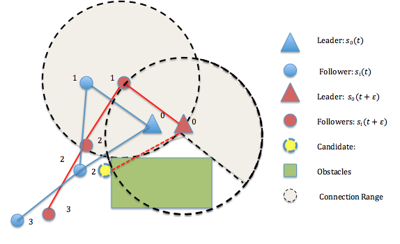
We propose an algorithm next to construct a connected graph, which may no longer be optimal in the sense of problem (9) but it does provide a valid initial condition for invoking the CPA described above (this is illustrated in Fig. 4 as the solid red graph). This immediately allows us to iteratively apply the CPA so as to obtain a new (locally optimal) formation.

Clearly, it is also possible to invoke (9) as soon as a formation reconfiguration is needed. However, the set $F$ is no longer convex and the computational complexity of this problem makes it infeasible for the on-line adaptation required, whereas the approach we propose and the use of the CPA render this process computationally manageable. In particular, whereas the MINLP is generally NP hard, in the CPA each agent $i$ determines its new position through a gradient-based scheme using only its neighbor set and its downstream and upstream agent sets relative to the leader (formally defined in the next section). When the number of agents increases, note that the the number of neighbors of $i$ may not be affected. The overall increase in complexity is linear in the network size.

Before proceeding, we identify the precise instants when formation reconfiguration is necessary due to obstacles encountered by agents as the mission unfolds over $[0,T]$. We define two states that the agent team can be in: $(i)$ The constrained state occurs when the sensing capability of an agent is hindered by an obstacle, captured by the condition $\left(\bigcup_{i=0}^{N}\Omega_{i}\right)\bigcap\left(\bigcup_{i=1}^{m}\mathring{M_{i}}\right)\neq\emptyset$, i.e., the intersection of the sensed part of $\Omega$ and the set of interior points of any obstacle is not empty, and $(ii)$ The free state corresponding to $\left(\bigcup_{i=0}^{N}\Omega_{i}\right)\bigcap\left(\bigcup_{i=1}^{m}\mathring{M_{i}}\right)=\emptyset$. Thus, the interval $[0,T]$ is partitioned into free and constrained intervals with transitions at times $t_{f}^{0}<t_{c}^{1}<t_{f}^{1}<...<t_{c}^{i}<t_{f}^{i}<...t_{f}^{z}<T$. This is described in Fig. 5. Next, we consider how to generate optimal formations over different alternating intervals $[t_{f}^{k},t_{c}^{k+1})$ and $[t_{c}^{k+1},t_{f}^{k+1})$.

In this section, we provide a simulation example illustrating what the optimal formation maximizing coverage in a mission space with obstacles looks like and how it changes at some significant instants.

We choose the event density functions to be uniform, i.e., $R(x)=1$. The mission space is a $60\times 50$ rectangle. The distance constraint is $C=10$ and the sensing range of each agent is $\delta=8$. At every step, the leader moves to the right one distance unit per unit of time. The mission space is colored from dark to lighter as the joint detection probability decreases (the joint detection probability is $\geq 0.50$ for green areas, and near zero for white areas). The leader (labeled “L”) moves along a predefined trajectory (the purple dashed line). There are 8 followers, indicated by numbers, which are restricted to locations on the left side of the leader during any movement.

Figures 9-13 show snapshots of the process at selected events of interest over $[0,T]$. Figure 9 shows the initial configuration at $t=0$, where the agent team is located in a convex feasible space. As shown in Sec. III, in this case, the optimal formation can be obtained by solving a MINLP [25]. In the results shown, we have used TOMLAB, a MATLAB-based optimization solver. For the non-convex objective function defined in (12), the solution is usually a local maximum; we sought to find the best local (possibly global) optimum possible by implementing a multi-start algorithm on the solver. This is done at the start of the mission, when an off-line computationally intensive procedure is possible. Moreover, this local maximum can be improved by applying the CPA; in fact, in this example the use of the CPA led to an improvement from $H(\mathbf{s})=741.5$ to $H(\mathbf{s})=816.7$, as shown in Fig. 9. Thus, in general, supplying the CPA with an initial connected graph obtained by solving the MINLP enables it to converge to a better value. For example, Fig. 13 is a local maximum attained by starting with a star-like connected graph shown in Fig. 13 with the objective function value $H(\mathbf{s})=781.1$ (although this is still worse than the value in Fig. 9).

In the time interval $[0,5]$, the formation is maintained. At $t=5$, agent 5 is located at a vertex of an obstacle and will therefore lose connectivity as the leader moves to the next step at $t=6$. At this point, agent 5 will determine its next position $s_{5}(6)$ by applying a projection at Step 3 of Algorithm 1. Note that only agent 5 needs to perform this projection, rather than the whole team of agents, hence the computational effort is minimal. Figure 9 captures the optimal formation following Fig. 9.

Observe that over the period $[0,12)$, although the optimal formation remains a tree, it is no longer the same as the original one. However, for each agent $i$, its downstream node set $\mathscr{D}_{i}$ and upstream node set $\mathscr{U}_{i}$ remain unchanged. At $t=12$, clearly, the structure of the formation has been changed. This is a consequence of either the projection step in Algorithm 1 or the CPA. At the end of the mission at $t=35$, the formation is shown in Fig. 13. The agents seek to form a line to go through the narrow region of the mission space while at the same time maximizing coverage. During the remaining interval $[12,35]$, the process is similar to what is seen over $[5,12]$.

As we pointed out in the last section, constructing a connected graph can be accomplished in a variety of ways. As shown in Fig. 13, a star-like graph is an inferior formation to that of Fig. 9; this is expected since the latter was obtained specifically to maximize the objective function in (12). In addition, a reconfiguration process as shown in Fig. 13 requires agents to move longer distances, hence consuming more energy.

We have addressed the issue of optimal dynamic formation of multi-agent systems in mission spaces with obstacles. When the agent team is in a free state (no obstacles in the mission space affecting them), a locally optimal solution of a MINLP can provide an initial formation that agents maintain or it is a good initial point for using the CPA (developed in prior work [18]) to obtain a better local optimum. When the feasible space is non-convex and connectivity is lost, we have developed an algorithm to construct a connected graph as an input for the CPA while seeking to maintain the original formation with minimal effort.

Future work aims at investigating optimal dynamic formation control for more general classes of objective functions, beyond the coverage control problem.

References

- [1] Y. Cao, W. Yu, W. Ren, and G. Chen, “An overview of recent progress in the study of distributed multi-agent coordination,” IEEE Transactions on Industrial Informatics, vol. 9, no. 1, pp. 427–438, Feb 2013.
- [2] C. Boutilier, “Sequential optimality and coordination in multiagent systems,” in In International Joint Conference on Artificial Intelligence, vol. 99, 1999, pp. 478–485.
- [3] R. W. Beard, J. Lawton, F. Y. Hadaegh et al., “A coordination architecture for spacecraft formation control,” IEEE Transactions on control systems technology, vol. 9, no. 6, pp. 777–790, 2001.
- [4] J. Shamma, Cooperative Control of Distributed Multi-Agent Systems. New York, NY, USA: Wiley-Interscience, 2008.
- [5] J. Choi, S. Oh, and R. Horowitz, “Distributed learning and cooperative control for multi-agent systems,” Automatica, vol. 45, no. 12, pp. 2802 – 2814, 2009.
- [6] C. G. Cassandras and W. Li, “Sensor networks and cooperative control,” European Journal of Control, vol. 11, no. 4-5, pp. 436–463, 2005.
- [7] M. Cao, A. Morse, C. Yu, B. Anderson, and S. Dasgupta, “Maintaining a directed, triangular formation of mobile autonomous agents,” Communications in Information and Systems, vol. 11, no. 1, p. 1, 2011.
- [8] K.-K. Oh and H.-S. Ahn, “Formation control and network localization via orientation alignment,” IEEE Transactions on Automatic Control, vol. 59, no. 2, pp. 540–545, Feb 2014.
- [9] J. Desai, V. Kumar, and J. Ostrowski, “Control of changes in formation for a team of mobile robots,” in Proc. of the IEEE International Conference on Robotics and Automation, vol. 2, 1999, pp. 1556–1561 vol.2.
- [10] H. Yamaguchi and T. Arai, “Distributed and autonomous control method for generating shape of multiple mobile robot group,” in Proc. of the IEEE International Conference on Intelligent Robots and Systems, vol. 2, Sep 1994, pp. 800–807 vol.2.
- [11] J. Wang and M. Xin, “Integrated optimal formation control of multiple unmanned aerial vehicles,” IEEE Transactions on Control Systems Technology, vol. 21, no. 5, pp. 1731–1744, Sept 2013.
- [12] M. Ji and M. B. Egerstedt, “Distributed coordination control of multi-agent systems while preserving connectedness.” IEEE Transactions on Robotics, vol. 23, no. 4, pp. 693–703, 2007.
- [13] S. Meguerdichian, F. Koushanfar, M. Potkonjak, and M. Srivastava, “Coverage problems in wireless ad-hoc sensor networks,” in Proc. of 20th Annual Joint Conf. of the IEEE Computer and Commun. Societies, vol. 3, 2001, pp. 1380–1387.
- [14] J. Cortes, S. Martinez, T. Karatas, and F. Bullo, “Coverage control for mobile sensing networks,” IEEE Transactions on Robotics and Automation, vol. 20, no. 2, pp. 243–255, 2004.
- [15] C. Caicedo-Nuez and M. Zefran, “A coverage algorithm for a class of non-convex regions,” in Proc. of the 47th IEEE Conf. on Decision and Control, 2008, pp. 4244–4249.
- [16] C. H. Caicedo-Nunez and M. Zefran, “Performing coverage on nonconvex domains,” in Proc. of the 2008 IEEE Conf. on Control Applic., 2008, pp. 1019–1024.
- [17] A. Breitenmoser, M. Schwager, J.-C. Metzger, R. Siegwart, and D. Rus, “Voronoi coverage of non-convex environments with a group of networked robots,” in Proc. of the 2010 IEEE International Conference on Robotics and Automation, 2010, pp. 4982–4989.
- [18] M. Zhong and C. Cassandras, “Distributed coverage control and data collection with mobile sensor networks,” IEEE Transactions on Automatic Control, vol. 56, no. 10, pp. 2445–2455, 2011.
- [19] A. Gusrialdi and L. Zeng, “Distributed deployment algorithms for robotic visual sensor networks in non-convex environment,” in 2011 IEEE International Conference on Networking, Sensing and Control (ICNSC), April 2011, pp. 445–450.
- [20] X. Sun, C. Cassandras, and K. Gokbayrak, “Escaping local optima in a class of multi-agent distributed optimization problems: A boosting function approach,” in Proc. of the IEEE 53rd Annual Conference on Decision and Control, Dec 2014, pp. 3701–3706.
- [21] M. Schwager, F. Bullo, D. Skelly, and D. Rus, “A ladybug exploration strategy for distributed adaptive coverage control,” in Proc. of the IEEE International Conference on Robotics and Automation, 2008, pp. 2346–2353.
- [22] A. Gusrialdi, R. Dirza, T. Hatanaka, and M. Fujita, “Improved distributed coverage control for robotic visual sensor network under limited energy storage,” Int. J. Imaging Robot, vol. 10, no. 2, pp. 58–74, 2013.
- [23] R. Merris, “Laplacian matrices of graphs: a survey,” Linear algebra and its applications, vol. 197, pp. 143–176, 1994.
- [24] R. Olfati-Saber and R. Murray, “Consensus problems in networks of agents with switching topology and time-delays,” IEEE Transactions on Automatic Control, vol. 49, no. 9, pp. 1520–1533, Sept 2004.
- [25] M. R. Bussieck and S. Vigerske. (2014, March) Minlp solver software. [Online]. Available: http://www.math.hu-berlin.de/~stefan/minlpsoft.pdf.