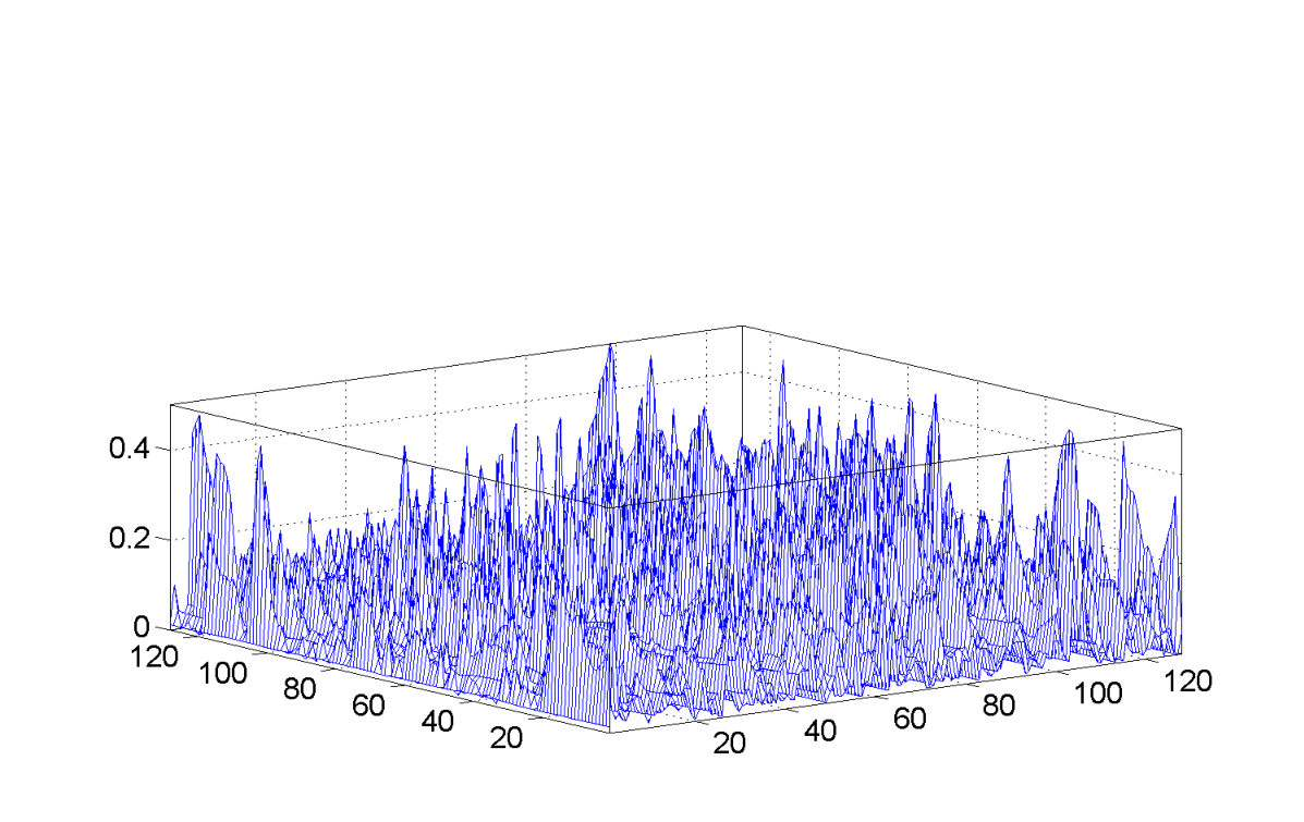
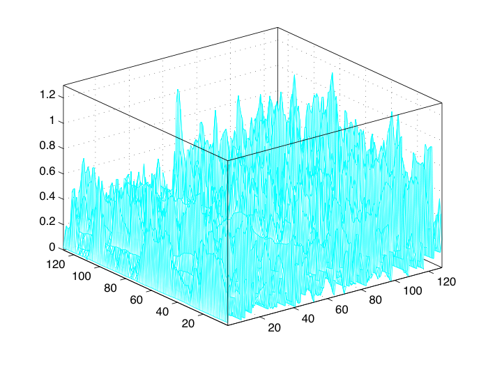
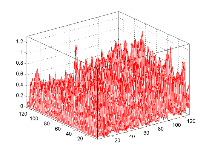
Compression and Recovery of Distributed Random Signals

We seek to find effective numerical algorithms for an information processing scenario that involves a set of spatially distributed sensors, $\mathcal{Q}_{1},\ldots,\mathcal{Q}_{p}$, and a fusion center, $\cal P$. The sensors make local observations, ${\bf y}_{1},\ldots,{\bf y}_{p}$, which are noisy versions of a signal of interest, ${\bf x}$. Each sensor $\mathcal{Q}_{j}$ transmits compressed information ${\bf u}_{j}$ about its measurements to the fusion center which should recover the original signal within a prescribed accuracy. Such an information processing relates to a wireless sensor network (WSN) scenario. In the recent years, research and development on new and refined WSN techniques has increased at a remarkable rate (see, for example, [6, 7, 8, 9, 10, 11, 12]). This is, in particular, because of a multitude of WSN applications due to their low deployment and maintenance cost.

The key problem is to to find an effective way to compress and denoise each observation ${\bf y}_{j}$, where $j=1,\ldots,p$, and then reconstruct all the compressed observations in the fusion center so that the reconstruction will be optimal in the sense of a minimization of the associated error under a certain criterion, such as the mean square error (MSE). A restriction is that the sensors cannot communicate with each other. Here, the term “compression” is treated in the same sense as in the known works on data compression (developed, for instance, in [13, 14, 15, 16]), i.e. we say that observed signal ${\bf y}_{j}$ with $n_{j}$ components is compressed if it is represented as signal ${\bf u}_{j}$ with $r_{j}$ components where $r_{j}<n_{j}$, for $j=1,\ldots,p$. That is “compression” refers to dimensionality reduction and not quantization which outputs bits for digital transmission. This is similar to the way considered, in particular, in [17].

It is known that in the nondisrtibuted setting (in the other words, in the case of a single sensor only) the MSE optimal solution is provided by the Karhunen-Loève transform (KLT) [13, 14, 18, 3]. Nevertheless, the classical KLT cannot be applied to the above WSN since the entire data vector ${\bf y}=[{\bf y}_{1}^{T},\ldots,y_{p}^{T}]^{T}$ is not observed by each sensor. Therefore, several approaches to a determination of mathematical models for $\mathcal{Q}_{1},\ldots,\mathcal{Q}_{p}$ and $\cal P$ have been pursued. In particular, in the information-theoretic context, distributed compression has been considered in the landmark works of Slepian and Wolf [19], and Wyner and Ziv [20]. A transform-based approach to distributed compression and the subsequent signal recovery has been considered in [11, 17, 21, 22, 23, 24]. Intimate relations between these two perspectives have been shown in [25]. The methodology developed in [17, 21, 22, 23, 24] is based on the dimensionality reduction by linear projections. Such an approach has received considerable attention (see, for example, [6, 7, 8, 10, 26, 27]).

In this paper, we consider a further extension of the methodology studied in [17, 21, 22, 23, 24]. In particular, in [17], two approaches are considered. By the first approach, the fusion center model, $\cal P$, is given in the form $\mbox{$\cal P$}=[\mbox{$\cal P$}_{1},\ldots,\mbox{$\cal P$}_{p}]$ where $\mbox{$\cal P$}_{j}$ is a ‘block’ of $\cal P$, for $j=1,\ldots,p$, and then the original MSE cost function is represented as a sum of $p$ decoupled MSE cost functions. Then approximations to $\mathcal{Q}_{j}$ and $\mbox{$\cal P$}_{j}$ are found as solution to each of the $p$ associated MSE minimization (MSEM) problems. We observe that the original MSE cost function and the sum of $p$ decoupled MSE cost functions are not equivalent. This is because the covariance matrix cannot be represented in a block diagonal form in the way presented in [17]. Some more related explanations can be found in [28]. Therefore, the first approach in [17] leads to the corresponding increase in the associated error. The second approach in [17] generalizes the results in [21, 22] in the following way. The original MSE cost function is represented, by re-grouping its terms, in the form similar to that presented by a summand in the decoupled MSE cost function. Then the minimum is seeking for each $\mbox{$\cal P$}_{j}\mathcal{Q}_{j}$ , for $j=1,\ldots,p$, while other terms $\mbox{$\cal P$}_{k}\mathcal{Q}_{k}$, for $k=1,\ldots,j-1,j+1,\ldots,p$, are assumed to be fixed. The minimizer follows from the known result given in [29] (Theorem 10.2.4). While the original MSEM problem is stated for a simultaneous determination of $\mathcal{Q}_{1},\ldots,\mathcal{Q}_{p}$ and $\cal P$, the approach in [17] requires to solve $p$ local MSEM problems which are not equivalent to the original problem. To combine solutions of those $p$ local MSEM problems, approximations to each sensor model $\mathcal{Q}_{j}$ are determined from an iterative procedure. Values of $\mathcal{Q}_{1},\ldots,\mathcal{Q}_{p}$ for the initial iteration are chosen randomly.

The approach in [24] is based on the ideas similar to those in the earlier references [17, 21, 22, 23]¹¹ 1 In particular, it generalizes work [23] to the case when the vectors of interest do not to be directly observed at the sensors., i.e. on the replacement of the original MSEM problem with the $p+1$ unconstrained MSEM problems for separate determination of approximations to $\mathcal{Q}_{j}$ , for each $j=1,\ldots,p$, and then an approximation to $\cal P$. First, an approximation to each $\mathcal{Q}_{j}$ , for $j=1,\ldots,p$, is determined under assumption that other $p-1$ sensors are fixed. Then, on the basis of known approximations to $\mathcal{Q}_{1},\ldots,\mathcal{Q}_{p}$, an approximation of $\cal P$ is determined as the optimal Wiener filter. Those $p+1$ problems considered in [24] are not equivalent to the original problem. In [24], the involved signals are assumed to be zero-mean jointly Gaussian random vectors. Here, this restriction is not used.

The work in [21, 22, 23] can be considered as a particular case of [24].

The method in [11] is applied to the problem which is an approximation of the original problem. It implies an increase in the associated error compared to the method applied to the original problem. Further, it is applicable under certain restrictions imposed on observations and associated covariance matrices. In particular, in [11], the observations should be presented in the special form ${\bf y}_{j}=H_{j}\mbox{$\mathbf{x}$}+\mbox{$\mathbf{v}$}_{j}$, for $j=1,\ldots,p$ (where $H_{j}$ is a measurement matrix and $\mbox{$\mathbf{v}$}_{j}$ is noise), and the covariance matrix formed by the noise vector should be block-diagonal and invertible. It is not the case here.

The WSN models in [11, 17, 21, 22, 23, 24] are justified in terms of inverse matrices. It is known that in the cases when the matrices are close to singular this may lead to instability and significant increase in the associated error. Moreover, when the matrices are singular, the algorithms [17, 21, 22, 23, 24] may not be applicable. This observation is illustrated by Examples 2, 3 and 4 in Section VI below where the associated matrices are singular and the method [17] is not applicable. Although in [24], for the case when a matrix is singular, it is proposed to replace its inverse by the pseudo-inverse, such a simple replacement does not follow from the justification of the model provided in [24]. As a result, a simple substitution of the pseudo-inverse matrices instead of the inverse matrices may lead to the numerical instability as it is shown, in particular, in Example 4 in Section VI. In this regard, we also refer to references [3, 4, 30] where the case of rank-constrained data compression in terms of the pseudo-inverse matrices is studied.

Thus, methods in [17, 21, 22, 23, 24, 11] are justified only for full rank matrices used in the associated models. This is not the case here. On the basis of the methodology developed in [3, 4, 30], our method is rigorously justified for models with matrices of degenerate ranks (Sections III-A and VIII).

Further, the second approach in [17] is, in fact, the block coordinate descent (BCD) method [31]. The BCD method converges (to a local minimum) under the assumptions that the objective function and the space of optimization need to be convex or the minimum of the objective function is uniquely attended (see [31] and [32], p. 267). Those conditions are not satisfied for our method (as for the method in [17] as well). Unlike the BCD method [31] used in [17], the maximum block improvement (MBI) method [1, 2] avoids the requirements of the BCD method. The MBI method guaranties convergence to a coordinate-wise minimum point which is a local minimum of the objective function. Therefore, the approach proposed in this paper is based, in particular, on the idea of the MBI method.

As distinct from the technique in [11] our method is applied to the original minimization problem, not to an approximation of the original problem as in [11]. It allows us to avoid the increase in the associated error. We also do not impose any of the restrictions on our method as those in [11] mentioned in Section I-B above. In particular, we do not assume that the covariance matrix formed by the noise vector should be block-diagonal.

The methods in [17, 21, 22, 23, 24] have been developed under assumption that exact covariance matrices are known. A knowledge of exact covariance matrices might be a restrictive condition in some cases, in particular, when matrices are large. In this paper, these difficulties are mitigated to some extent.

Key advantages of the proposed method are as follows. The method represents a combination of the generic Karhunen-Loève transform (KLT) [3] (based on the work in [5]) and the MBI method [1, 2]. Therefore, it unites the merits of both techniques [3, 5] and [1, 2]. As a result, our approach provides, in particular, the minimal MSE at each step of the version of the MBI method we use. The WSN model is represented in the form called the multi-compressor KLT-MBI transform and is based on the ideas which are different from those used in known methods [6, 7, 8, 10, 17, 21, 22, 23, 24, 26]. The multi-compressor KLT-MBI is given in terms of pseudo-inverse matrices and, therefore, it is numerically stable and always exists. In other words, the proposed WSN model provides compression, de-noising and reconstruction of distributed signals for the cases when known methods either are not applicable (because of singularity of associated matrices) or produce larger associated errors. This observation is supported, in particular, by results of simulations in Section VI.

Here, we provide some notation which is required to formalize the problem in the form presented in Section II-B below. Let us write $(\Omega,\Sigma,\mu)$ for a probability space²² 2 $\Omega=\{\omega\}$ is the set of outcomes, $\Sigma$ a $\sigma-$field of measurable subsets of $\Omega$ and $\mu:\Sigma\rightarrow[0,1]$ an associated probability measure on $\Sigma$ with $\mu(\Omega)=1$.. We denote by ${\bf x}\in L^{2}(\Omega,\mathbb{R}^{m})$ the signal of interest³³ 3 The space $L^{2}(\Omega,\mathbb{R}^{m})$ has to be used because of the norm introduced below in (5). (a source signal to be estimated) represented as ${\bf x}=[{\bf x}^{(1)},\ldots,{\bf x}^{(m)}]^{T}$ where ${\bf x}^{(j)}\in L^{2}(\Omega,\mathbb{R})$, for $j=1,\ldots,m$. Futher, ${\bf y}_{1}\in L^{2}(\Omega,\mathbb{R}^{n_{1}}),\ldots,{\bf y}_{p}\in L^{2}(\Omega,\mathbb{R}^{n_{p}})$ are observations made by the sensors where $n_{1}+\ldots+n_{p}=n$. In this regard, we write

where ${\bf y}^{(k)}\in L^{2}(\Omega,\mathbb{R})$, for $k=1,\dots,n$. We would like to emphasize a difference between ${\bf y}_{j}$ and $\mbox{$\mathbf{y}$}^{(k)}$: in (1), the observation ${\bf y}_{j}$, for $j=1,\dots,p$, is a ‘piece’ of random vector ${\bf y}$ (i.e. ${\bf y}_{j}$ is a random vector itself), and ${\bf y}^{(k)}$, for $k=1,\ldots,n$ is an entry of y (i.e. ${\bf y}^{(k)}$ is a random variable).⁴⁴ 4 Therefore, $\mbox{$\mathbf{y}$}_{j}=[\mbox{$\mathbf{y}$}^{(n_{0}+n_{1}+\ldots+n_{j-1})},\ldots,\mbox{$\mathbf{y}$}^{(n_{1}+\ldots+n_{j})}]^{T}$ where $j=1,\ldots,p$ and $n_{0}=1$.

For $j=1,\ldots,p$, let us define a sensor model $\mathcal{Q}_{j}:L^{2}(\Omega,\mathbb{R}^{n_{j}})\rightarrow L^{2}(\Omega,\mathbb{R}^{r_{j}})$ by the relation

where $Q_{j}\in\mathbb{R}^{r_{j}\times n_{j}}$,

Let us denote ${\bf u}_{j}=\mathcal{Q}_{j}({\bf y}_{j})$ and ${\bf u}=[{\bf u}^{T}_{1},\ldots,{\bf u}^{T}_{p}]^{T}$, where for $j=1,\ldots,p$, vector ${\bf u}_{j}\in L^{2}(\Omega,\mathbb{R}^{r_{j}})$ represents the compressed and filtered information vector transmitted by a $j$th sensor $\mathcal{Q}_{j}$ to the fusion center $\cal P$. A fusion center model is defined by $\mbox{$\cal P$}:L^{2}(\Omega,\mathbb{R}^{r})\rightarrow L^{2}(\Omega,\mathbb{R}^{m})$ so that

where $P\in\mathbb{R}^{m\times r}$ and ${\bf u}\in L^{2}(\Omega,\mathbb{R}^{r})$. To state the problem in the next section, we also denote

where $\|{\bf x}(\omega)\|_{2}$ is the Euclidean norm of ${\bf x}(\omega)\in\mathbb{R}^{m}$. For convenience, we will use notation $\|{\bf x}\|^{2}_{\Omega}$, not $\mbox{$\mathbb{E}$}\left[\|{\bf x}(\omega)\|_{2}^{2}\right]$, to denote the norm in (5).

For the WSN depicted in Fig. 1, the problem can be stated as follows: Find models of the sensors, $\mathcal{Q}_{1},\ldots,\mathcal{Q}_{p}$, and a model of the fusion center, $\cal P$, that provide

under the assumption that $\mathcal{Q}_{1},\ldots,\mathcal{Q}_{p}$ and $\cal P$ are given by (2) and (4), respectively. The model of the fusion center, $\cal P$, can be represented as $\mbox{$\cal P$}=[\mbox{$\cal P$}_{1},\ldots,\mbox{$\cal P$}_{p}]$ where $\mbox{$\cal P$}_{j}:L^{2}(\Omega,\mathbb{R}^{r_{j}})\rightarrow L^{2}(\Omega,\mathbb{R}^{m})$, for $j=1,\ldots,p$. Let us write

where $\mbox{$\mathbf{y}$}=[{\bf y}_{1}^{T},\ldots,{\bf y}_{p}^{T}]^{T}.$

For $j=1,\ldots,p$, let us denote $\mbox{$\cal F$}_{j}=\mbox{$\cal P$}_{j}\mbox{$\cal Q$}_{j}$. We also write $\mbox{$\cal F$}=[\mbox{$\cal F$}_{1},\ldots,\mbox{$\cal F$}_{p}]$. Then the WSN model can be represented as

Denote by $\mbox{$\cal R$}(m,n,k)$ the variety of all $m\times n$ linear operators of rank at most $k$. For the sake of simplicity we sometimes will also write $\mbox{$\cal R$}_{k}$ instead of $\mbox{$\cal R$}(m,n,k)$. The problem in (11) can equivalently be reformulated as follows: Find $\mbox{$\cal F$}_{1}\in\mathcal{R}(m,n_{1},r_{1}),$ $\ldots,$ $\mbox{$\cal F$}_{p}\in\mathcal{R}(m,n_{p},r_{p})$ that solve

Recall that $r_{j}<n_{j}$, for $j=1,\ldots,p$.

Further, to simplify the notation we will use the same symbol to denote an operator and the associated matrix. For example, we write $Q_{j}$ to denote both the operator $\mathcal{Q}_{j}$ and matrix $Q_{j}$ introduced in (2). Similarly, we write $P_{j}$ to denote both operator $\mbox{$\cal P$}_{j}$ and matrix $P_{j}\in\mathbb{R}^{m\times r_{j}}$ introduced above, etc. In particular, by this reason, in (13) we will write $F_{j}$ , not $\mathcal{F}_{j}$ .

For ${\bf x}$ represented by ${\bf x}=[{\bf x}^{(1)},\ldots,{\bf x}^{(m)}]^{T}$ where $\mbox{$\mathbf{x}$}^{(j)}\in L^{2}(\Omega,\mathbb{R})$ we write

where $\displaystyle\langle{\bf x}^{(j)}{\bf y}^{(k)}\rangle=\int_{\Omega}{\bf x}^{(j)}(\omega){\bf y}^{(k)}(\omega)d\mu(\omega)$ and ${\bf y}=[{\bf y}^{(1)},\ldots,{\bf y}^{(n)}]^{T}$.

The assumption used in the known methods [6, 7, 8, 10, 11, 17, 21, 22, 23, 24, 26, 27] is that covariance matrices $E_{xy}$ and $E_{yy}$ are known. At the same time, in many cases, it is difficult to know exact values of $E_{xy}$ and $E_{yy}$. For instance, if it is assumed that signal $\mathbf{y}$ is a Gaussian random vector then the associated parameters $\rho$ and $\sigma^{2}$ for matrix $E_{yy}$ are still unknown (see [24] as an example). Therefore, we are mainly concerned with the case when estimates of $E_{xy}$ and $E_{yy}$ can be obtained. Methods of estimation of matrices $E_{xy}$ and $E_{yy}$ were studied in a number of papers (see, for example, [33, 34, 35, 36, 37, 38, 39, 40]) and it is not a subject of our work. In particular, samples of training signals taken for some different random outcomes $\omega$ might be available. Some knowledge of the covariances can also come from specific data models. Then the aforementioned covariance matrices can be estimated.

In the following Section III, we provide solutions in terms of both matrices $E_{xy}$, $E_{yy}$ and their estimates. The associated error analysis is given in Sections V and VIII.

Here, we recall the known result for the case of a single sensor, i.e. for $p=1$ in (6) and (13), and provide some related explanations which will be extended in the sections that follow.

The Moore-Penrose generalized inverse for a matrix $M$ is denoted by $M^{\dagger}$. We set $M^{1/2\dagger}=(M^{1/2})^{\dagger}$, where $M^{1/2}$ is a square root of $M$, i.e. $M=M^{1/2}M^{1/2}$. Then the known solution (see, for example [3]) of the particular case of problem (13), for $p=1$, is given by

where symbol $[\cdot]_{r_{1}}$ denotes a truncated singular value decomposition (SVD) taken with $r_{1}$ first nonzero singular values and matrix $M_{1}$ is arbitrary. The expression (15) represents the Karhunen-Loève transform as given, for example, in [6].

In (15), in particular, $M_{1}=\mathbb{O}$ where $\mathbb{O}$ is the zero matrix. Then $Q_{1}$ and $P_{1}$ that solve (6) follow from a decomposition of matrix $\left[E_{x,y_{1}}(E^{\dagger}_{y_{1}y_{1}})^{1/2}\right]_{r_{1}}(E^{\dagger}_{y_{1}y_{1}})^{1/2}$, based on the truncated SVD, in a product $P_{1}Q_{1}$ of $r_{1}\times n$ matrix $Q_{1}$ and $m\times r_{1}$ matrix $P_{1}$ , respectively.

We will extend this argument in Section III below for a general case with more than one sensor.

We wish to find $F_{1},\ldots,F_{p}$ that provide a solution to the problem (13) for an arbitrary finite number of sensors in the WSN model, i.e. for $p=1,2,\ldots$ in (13). To this end, we need some more preliminaries which are given in Sections III-A1 and III-A2 that follow. The method itself and an associated algorithm are then represented in Section III-A3.

The models of sensors $Q_{1},\ldots,Q_{p}$ and the fusion center $P=[P_{1},\ldots,P_{p}]$ of the WSN in Fig. 1 follow from the formula $F_{j}=P_{j}Q_{j}$ introduced in (12). By the proposed method, $F_{j}$ is represented by $F^{(q+1)}_{j}$ given by Algorithm 1 above. Therefore, the mathematical model of the WSN is given by

Here, ${F}^{(q+1)}_{j}={P}_{j}^{(q+1)}{Q}_{j}^{(q+1)}$ and ${P}^{(q+1)}=[{P}_{1}^{(q+1)},\ldots,{P}_{p}^{(q+1)}]$. Then ${Q}^{(q+1)}_{j}\in\mbox{$\mathbb{R}$}^{r_{j}\times n_{j}}$ and ${P}^{(q+1)}_{j}\in\mbox{$\mathbb{R}$}^{m\times r_{j}}$ follow from the SVD decomposition of matrix ${F}^{(q+1)}_{j}$ taken with $r_{j}$ first nonzero singular values. This procedure has been described in Section II-D for the case of only one sensor, i.e. for $p=1$.

For the case when instead of matrices $E_{xy}$ and $E_{yy}$ their estimates $\widetilde{E}_{xy}$ and $\widetilde{E}_{yy}$ are used, the models are constructed by the similar procedure with the replacement of $F^{(q+1)}_{j}$ by $\widetilde{F}^{(q+1)}_{j}$ (see Remark 2 above).

Note that the proposed WSN model also provides de-noising of observations ${\bf y}_{1},\ldots,{\bf y}_{p}$.

References

- [1] B. Chen, S. He, Z. Li, S. Zhang, Maximum block improvement and polynomial optimization, SIAM Journal on Optimization 22 (1) (2012) 87–107.
- [2] Z. Li, A. Uschmajew, S. Zhang, On convergence of the maximum block improvement method, SIAM Journal on Optimization 25 (1) (2015) 210–233.
- [3] A. Torokhti, P. Howlett, Computational Methods for Modelling of Nonlinear Systems, Elsevier, 2007.
- [4] S. Friedland, A. Torokhti, Generalized rank-constrained matrix approximations, SIAM Journal on Matrix Analysis and Applications 29 (2) (2007) 656–659.
- [5] A. Torokhti, S. Friedland, Towards theory of generic Principal Component Analysis, Journal of Multivariate Analysis 100 (4) (2009) 661 – 669.
- [6] P. L. Dragotti, M. Gastpar, Distributed Source Coding: Theory, Algorithms and Applications, Academic Press, 2009.
- [7] J. Fang, H. Li, Optimal/near-optimal dimensionality reduction for distributed estimation in homogeneous and certain inhomogeneous scenarios, IEEE Transactions on Signal Processing 58 (8) (2010) 4339–4353.
- [8] A. Amar, A. Leshem, M. Gastpar, Recursive implementation of the distributed Karhunen-Loeve transform, IEEE Transactions on Signal Processing 58 (10) (2010) 5320–5330.
- [9] A. Bertrand, M. Moonen, Distributed adaptive node-specific signal estimation in fully connected sensor networks—part i: Sequential node updating, IEEE Transactions on Signal Processing 58 (10) (2010) 5277 – 5291.
- [10] M. Lara, B. Mulgrew, Performance of the distributed KLT and its approximate implementation, in: 2012 Proceedings of the 20th European Signal Processing Conference (EUSIPCO), 2012, pp. 724–728.
- [11] H. Ma, Y.-H. Yang, Y. Chen, K. Liu, Q. Wang, Distributed state estimation with dimension reduction preprocessing, Signal Processing, IEEE Transactions on 62 (12) (2014) 3098–3110.
- [12] D. E. Marelli, M. Fu, Distributed weighted least-squares estimation with fast convergence for large-scale systems, Automatica 51 (0) (2015) 27 – 39.
- [13] L. L. Scharf, The SVD and reduced rank signal processing, Signal Processing 25 (2) (1991) 113 – 133.
- [14] Y. Hua, W. Liu, Generalized Karhunen-Loeve transform, IEEE Signal Processing Letters 5 (6) (1998) 141–142.
- [15] Y. Hua, M. Nikpour, P. Stoica, Optimal reduced-rank estimation and filtering, IEEE Transactions on Signal Processing 49 (3) (2001) 457–469.
- [16] A. Torokhti, S. Miklavcic, Data compression under constraints of causality and variable finite memory, Signal Processing 90 (10) (2010) 2822 – 2834.
- [17] I. D. Schizas, G. B. Giannakis, Z.-Q. Luo, Distributed estimation using reduced-dimensionality sensor observations, IEEE Transactions on Signal Processing 55 (8) (2007) 4284–4299.
- [18] A. Torokhti, P. Howlett, Optimal fixed rank transform of the second degree, IEEE Trans. CAS. Part II, Analog and Digital Signal Processing 48 (3) (2001) 309 – 315.
- [19] D. Slepian, J. Wolf, Noiseless coding of correlated information sources, IEEE Transactions on Information Theory 19 (4) (1973) 471–480.
- [20] A. Wyner, J. Ziv, The rate-distortion function for source coding with side information at the decoder, IEEE Transactions on Information Theory 22 (1) (1976) 1–10.
- [21] E. Song, Y. Zhu, J. Zhou, Sensors optimal dimensionality compression matrix in estimation fusion, Automatica 41 (12) (2005) 2131 – 2139.
- [22] Y. Zhu, E. Song, J. Zhou, Z. You, Optimal dimensionality reduction of sensor data in multisensor estimation fusion, IEEE Transactions on Signal Processing 53 (5) (2005) 1631–1639.
- [23] M. Gastpar, P. Dragotti, M. Vetterli, The distributed Karhunen-Loève transform, IEEE Transactions on Information Theory 52 (12) (2006) 5177–5196.
- [24] O. Roy, M. Vetterli, Dimensionality reduction for distributed estimation in the infinite dimensional regime, IEEE Transactions on Information Theory 54 (4) (2008) 1655–1669.
- [25] V. Goyal, Theoretical foundations of transform coding, IEEE Signal Processing Magazine 18 (5) (2001) 9–21.
- [26] I. D. Schizas, A. Ribeiro, G. B. Giannakis, Dimensionality reduction, compression and quantization for distributed estimation with wireless sensor networks, in: Wireless Communications, Vol. 143 of The IMA Volumes in Mathematics and its Applications, Springer New York, 2007, pp. 259–296.
- [27] J. A. Saghri, S. Schroeder, A. G. Tescher, Adaptive two-stage Karhunen-Loeve-transform scheme for spectral decorrelation in hyperspectral bandwidth compression, Optical Engineering 49 (5) (2010) 057001–057001–7.
- [28] V. Ejov, A. Torokhti, How to transform matrices ,…, to matrices ,…, so that if ?, Numerical Algebra, Control and Optimization 2 (2) (2012) 293–299.
- [29] D. R. Brillinger, Time Series: Data Analysis and Theory, Holden Day, San Francisco, 2001.
- [30] A. Torokhti, S. Friedland, Towards theory of generic principal component analysis, Journal of Multivariate Analysis 100 (4) (2009) 661 – 669.
- [31] P. Tseng, Convergence of a block coordinate descent method for nondifferentiable minimization, Journal of Optimization Theory and Applications 109 (3) (2001) 475–494.
- [32] D. Bertsekas, Nonlinear Programming, Athena Scientific, 1995.
- [33] L. Perlovsky, T. Marzetta, Estimating a covariance matrix from incomplete realizations of a random vector, IEEE Transactions on Signal Processing 40 (8) (1992) 2097–2100.
- [34] O. Ledoit, M. Wolf, A well-conditioned estimator for large-dimensional covariance matrices, Journal of Multivariate Analysis 88 (2) (2004) 365 – 411.
- [35] O. Ledoit, M. Wolf, Nonlinear shrinkage estimation of large-dimensional covariance matrices, Ann. Statist. 40 (2) (2012) 1024–1060.
- [36] R. Adamczak, A. E. Litvak, A. Pajor, N. Tomczak-Jaegermann, Quantitative estimates of the convergence of the empirical covariance matrix in log-concave ensembles, Journal of the American Mathematical Society (23) (2009) 535–561.
- [37] R. Vershynin, How close is the sample covariance matrix to the actual covariance matrix?, Journal of Theoretical Probability 25 (3) (2012) 655–686.
- [38] S.-J. K. Joong-Ho Won, Johan Lim, B. Rajaratnam, Condition-number-regularized covariance estimation, Journal of the Royal Statistical Society: Series B (Statistical Methodology) 75 (3) (2013) 427–450.
- [39] B. W. Schmeiser, M. H. Chen, On hit-and-run Monte Carlo sampling for evaluating multidimensional integrals, Technical Report 91-39, Dept. Statistics, Purdue Univ.
- [40] R. Yang, J. O. Berger, Estimation of a covariance matrix using the reference prior, The Anna1s of Statistics 22 (3) (1994) 1195–1211.
- [41] L. Tu, An Introduction to Manifolds, Universitext, Springer, 2007.