Holographic dual of a time machine
Abstract
We apply the holography to the simplest possible eternal time machine solution in based on two conical defects moving around their center of mass along a circular orbit. Closed timelike curves in this space-time extend all the way to the boundary of , violating causality of the boundary field theory. By use of the geodesic approximation we address the “grandfather paradox” in the dual dimensional field theory and calculate the two-point retarded Green function. It has a non-trivial analytical structure both at negative and positive times, providing us with an intuition on how an interacting quantum field could behave once causality is broken. In contrast with the previous considerations our calculations reveal the possibility of a consistent and controllable evolution of a quantum system without any need to impose additional consistency constraints.
I Introduction
Solutions to the equations of General Relativity that describe space-times containing closed timelike curves (CTC) have attracted significant interest as they revealed at least hypothetical theoretical possibility of travelling in time. Since the renowned publication by Kurt Gödel [1] a number of causality violating solutions in GR as well as in modified theories of gravity have been constructed, among which we can name the Tipler-Van Stockum time machine generated by axially rotating distribution of particles [2], [3], the Morris-Thorne-Yurtsever transversable wormhole [4, 5], the Gott time machine based on moving conical defects [6], the Ori dust solution [7], and the solutions in theories of gravity [8] and theories with non-minimal matter-curvature coupling [9].
All questions about physics of time machines that could be posed in principle fall into three general categories:
- •
Is there a physical way to create a time machine?
- •
Is there any time machine solution that can be stable?
- •
What dynamical behaviour would a physical system experience evolving in a time machine background?
None of the questions have yet received a definite answer.
The answer to the first question is believed to be negative. Extensive analysis of particular time machine solutions has demonstrated that in order to create a space-time with CTC one needs matter that violates strong, weak or null energy conditions of General Relativity (different solutions require violation of different energy conditions), and only eternal time machines can exist [10, 11]. However we can not be sure that all matter in the Universe obeys these conditions. For instance, there are a number of models of the dark energy violating the null energy condition [12, 13, 14, 15], and this provides a way to by-pass the no-go statement.
The second question was raised by Hawking in [16], where he conjectured that a space-time with CTC can be stable only on classical level, but will be unavoidably destroyed by quantum fluctuations of the metric. The real universal proof or refutal of the conjecture can be obtained only within a framework of a complete theory of quantum gravity. String theory opened a possibility to check the chronology protection condition in specific cases. In [17] authors have shown that appearance of closed timelike curves in a certain (O-plane) orbifold background would cause a Hagedorn transition that restructures the space-time transforming it into a chronologically safe configuration. So this result can be considered as a very accurate and nice supporting evidence in favour of the Hawking conjecture. On the other hand in [18, 19, 20], it was demonstrated that the Gödel type solutions can be smoothly embedded in the context of string theory. Closed timelike curves in that case are hidden behind the so called holographic screens and do not violate causality in the rest of the space-time. Thus the chronology is protected, but structure of the CTC remains unbroken by quantum effects. An intriguing observation has been made by authors of [21] and [22], that from the point of view of the AdS/CFT correspondence, the existence of CTC in the bulk can be related to negative or exceeding one fermionic probability in the boundary field theory.
The third category includes various types of the “grandfather paradox”. For a classical wave equation on a non-globally hyperbolic space with CTC the possibility of self-consistent dynamics was demonstrated in [23, 24]. Classical mechanical billiards and their self-consistency conditions have been studied in [25]. A basis of states of a free quantum field theory in the Gott time machine has been constructed in [26], where it was shown that the causality violation leads to an emergence of an effective non-unitary interaction in the theory. Non-unitarity of interacting field theories in time machines was analyzed in [27]. Some authors even argued that evolution of a physical system along closed timelike curves can be studied experimentally by mean of simulation of emergent gravity in metamaterials [28], or a qubit interacting with an older version of itself [29].
However the question about properties of an interacting quantum field theory in a time machine background remains open, though the real “grandfather paradox” can take place only in a self-interacting system. When the notions of time ordering and unitarity are absent from the very beginning, it is unclear how to formulate an interacting field theory. In this paper we address this problem and by use of the AdS/CFT correspondence provide a constructive solution to it. Here we stand on the position that even if the presence of CTC causes breaking of unitarity in the boundary field theory [22], it should not be regarded as a big problem as long as we can formulate a prescription how to solve the theory. When one is trying to get an insight into physics of paradoxical systems, it is not very useful to rely on the “common sense” intuition and corresponding fundamental principles.
The AdS/CFT correspondence provides an elegant way to address the paradox. In the large limit it relates quantum field theories to a classical gravity, and thus we can study properties of a quantum theory in the CTC background just by careful analysis of the dual Riemannian geometry, without any need to formulate special quantization rules that would be valid in the case of broken causality.
The paper is organized as follows. In the next section we introduce a simple set up for the time machine in . In Sec. III we discuss geodesic structure of the spacetime, and suggest that it could lead to non-trivial effects in the boundary field theory. In Sec. IV we introduce a notion of timelike quasigeodesics that will be then used for connecting timelike separated boundary points. Finally, in Sec. V we formulate a precise algorithm for the Green function evaluation, provide the results of numerical simulations, and discuss the related phenomenology.
II Time machine in
The eternal time machine solution in has been suggested by Gott and DeDeo in [30] (for similar solutions containing CTC but collapsing into a BTZ black hole see [31]). Here we briefly recall its structure closely following the original text.
The three dimensional global anti-de Sitter space-time can be thought of as a hypersurface
| (1) |
embedded in a four-dimensional flat space-time with a metric:
| (2) |
In the Schwarzschild coordinates the embedding formulas are
| (3) | |||||
where .
The induced metric is then
| (4) |


A massive particle put into a three dimensional space-time removes a wedge with an angle deficit proportional to the mass of the particle, and edges (faces) emerging from this point-like particle. Points on the opposite edges of the wedge are identified, and the resulting space-time contains a conical defect, Fig.1(a). When we are looking at the unfolding of the conical defect, coordinate locations of the edges do not have an independent physical meaning, and we are free to rotate them preserving the angular deficit. For our purposes it will be convenient to make the cut out “pizza slice” twist in time with a constant angular velocity in the reference frame of the massive particle, making a full rotation in a period , Fig.1(b). Then for the trailing and leading faces of the wedge in the embedding coordinates we get:
Here is the angular deficit of the conical spacetime. Integrating the spacetime stress-energy tensor over the angle, we can deduce that the effective mass concentrated in the interior of the bulk is
| (5) |
Here the second term is the mass of the point-like source, and the first one is the contribution from the negative curvature.
For a single static conical defect we can not make its angular deficit larger than . If the mass of the point-like particle exceeds the limit (), the resulting space-time will be rather a BTZ black hole instead of a naked conical singularity [32].


However, if we boost the massive source, the removed wedge is effectively getting “squeezed” from the point of view of an external observer at rest (see Fig. 2(a)). This provides a room for a second conical defect with a deficit angle such that . In other words, relative motion can support the system of conical defects, preventing them from collapsing into a black hole. This will be the essence of the DeDeo-Gott construction.
Consider a system of two identical conical defects undergone two opposite Lorentz transformations, in the and planes of the embedding space each:
| (6) |
In the three-dimensional coordinates of the spacetime these Lorentzian transformations correspond to isometry transformations.
It can be shown that in the coordinates of global these defects move along the same circular orbit with a constant velocity, always being at the opposite points of the orbit, Fig.2(b). A conical defect sits at in its rest frame, i.e.
| (7) |
In the boosted frame
| (8) |
hence
| (9) | |||||
| (10) |
In the rest frame of a wedge, the points on its edges are identified at equal coordinate times. However if we boost it, from the point of view of an external observer this identification would occur at different times leading to time jumps for a particle moving around the conical singularity. In the case of a single conical defect its boost can be regarded as a global coordinate transformation of the space-time, which obviously can not cause any new physical effects. However, with two defects moving relative to each other, the relative time jumps become a physical effect that can not be eliminated by a (proper) choice of coordinate system. These time jumps allow for the existence of CTC.
Existence of closed timelike curves in this space-time can be demonstrated by looking at the identification of the edges near the boundary of (at ). We refer the reader to [30] for a detailed discussion, here we just quote the result. Speaking in terms of the unfolding of the two-conical space-time, when a timelike particle living on the boundary of the cylinder hits an edge of one of the two wedges, it undergoes a time and an angle jump:
| (11) | |||||
| (12) |
It can be shown that . If , the world line of the particle becomes a closed timelike curve, and thus the space-time is a time-machine, see Fig.3.
In the regime when this limit is not exceeded, and CTC are not present, the space-time has been studied in detail from holographic point of view in [33], but the case of broken causality has not been addressed.
In the next sections we will study geodesic structure of this time machine and explicitly show that in presence of the two orbiting conical defects we deal with a highly-nontrivial lensing of geodesics, and this reflects on the structure of two point Green’s functions of the dual boundary theory.
III Entwinement of geodesics and causality violations
When conformal dimension of a boundary operator in is very high, the corresponding two-point Green function can be derived in the geodesic approximation [32]:
| (13) |
where is the length of a geodesic connecting boundary points and . If there are more than one geodesic between and , they can give additional contributions to the propagator. This is the case for the DeDeo-Gott time machine geometry, and here we address possible outcome of this in details.
Consider two arbitrary points and located in the physical (unremoved) part of the boundary. Having two rotating conical defects in the bulk makes the structure of possible geodesics connecting11 1 When and are timelike separated we encounter some subtleties caused by the fact that in the space-time a timelike geodesic can not reach the boundary. These issues will be commented further on, but the general point of view described in this section remains unchanged. and very nontrivial, so we should find a way to calculate their contributions to the two-pont Green’s function . Let us shoot a geodesic from the boundary point to the point . Before it hits the point it can undergo a number of “refractions” on the faces of wedges, winding around either of two conical defects clockwise (if it hits the leading face of the wedge head on) or counterclockwise (if it overtakes the trailing face of the wedge from behind). For example, schematically a typical geodesic may have a structure (see also Fig. 4)
| (14) |
where stands for the act of clockwise/counterclockwise winding around the 1-st or the 2-nd wedge respectively.
So, formally the Green’s function in the geodesic approximation is given by
| (15) |
where the second sum is taken over all different entwinement structures corresponding to the same number of windings, and the first sum is taken over all winding numbers22 2 This idea of entwinements in holography has been introduced in [34], but there it was related to a concept of entanglement entropy “shadows” rather than to subleading contributions to the propagator.
It is easy to see that for a given number of windings the maximal possible number of topologically different geodesics is
| (16) |
The first winding act can be of four different types. But for each of the next steps, if a geodesic wrapped around a conical defect, for example, clockwise, then on the next step it can not go in the opposite direction and wrap around the same conical defect counterclockwise. It means that in the sequence of windings the winding act can be followed (at least hypothetically) by , but not by .
As we will see further, for a given pair of boundary points not all sequences of entwinements are physically realistic and can contribute to the sum (15).
To find a proper prescription for the lengths of the non-trivial winding geodesics let us discuss in detail a particular example.
Take a look at Fig.4. The length of the presented geodesic is a sum of lengths of its’ composing arcs:
| (17) |
We will refer to points as complementary points, and as refraction points. Coordinates of the refraction points are to be found from coordinates of and , and that can be easily done step by step.
Focus on the first refraction on the wedge, . The points of interest are . Here we neglect for a while the second wedge, so we do not consider the point at all, and we treat as a physical point (not just as a point in the complementary “removed” space), see Fig.5(a). These six points can be regarded as a result of boost transformation applied to the wedge. We can “unboost” the wedge and find static pre-images of these points (see Fig.5(b)). For the “unboosted” points the following relations trivially hold
| (18) | |||
where is a boundary identification vector proportional to the angular deficit. Here we subtract the identification vector because this particular entwinement is counterclockwise. For clockwise we should rather add . In that case points and are intersections of geodesics and with faces of the static wedge.
Applying the same procedure to the other entwinements, in a generic case we get a system of recurrent relations
| (19) | |||||
Here if the corresponding winding is . if the corresponding winding is . In these formulae we pick up the upper sign if , and the lower sign if .
Note, that the Lorentz boost we have defined in terms of the embedding space coordinates acts non-linearly on the points, therefore we can not simply expand the parentheses in (19).
Then for each of the auxiliary arcs we can derive coordinates of the refraction points , and write down corresponding lengths of the composing arcs.
Later we will also show that not every formally generated sequence of windings does exist.
IV Quasigeodesics connecting boundary points
To discuss causality properties of the dual boundary QFT, we will in particular need to consider boundary points with timelike separation. The conceptual problem we unavoidably encounter here is the absence of timelike geodesics connecting points on the conformal boundary of . The equations for timelike geodesics can be derived from the following Lagrangian for a massive particle in :
| (20) |
Such a particle has two conserved momenta:
| (21) | |||||
| (22) |
Substituting them into the Lagrangian we obtain the radial equation of motion:
| (23) | |||
| (24) |
Clearly the right hand side of the equation turns negative as , and thus no real solution to this equation can exist.
In the case of a stationary spacetime the obstacle could be easily surmounted by performing the analytic continuation of the metric to the Euclidean signature, calculating the Green function in terms of Euclidean lengths of the geodesics, and making the inverse Wick rotation back to real time. However in our case we deal with a spacetime that is not only non-stationary, but wich has no good global notion of time. Hence we are forced to stick to the Lorentzian time.
The way to implement the geodesic approximation for timelike separated boundary points in the single Poincaré patch has been suggested in [35]. Let’s turn for a second to the single patch of the spacetime, covered by the Poincaré coordinates:
| (25) |
Again, a massive bulk particle has two kinetic invariants:
| (26) | |||
| (27) |
but now we have two different classes of spacelike geodesics.
- •
For :
(28) - •
For :
(29)
We will be interested in the geodesics of the second kind. As these geodesics approach the point , which is the Poincaré horizon of the half- chart. Regarding the horizon as a single infinitely far point (as in the theory of complex functions), we can consider two disconnected spacelike geodesics possessing the same kinetic invariants and , but emerging from two different timelike separated boundary points and , as two branches of a single geodesic reaching the spatial infinity and returning back to the boundary. The length of such a geodesic will be divergent not only as (the standard holographic UV divergence), but also as , but this can be cured by an appropriate renormalization33 3 For details see App. B and D of [35]. The resulting expression for the renormalized length of the geodesic is simply
| (30) |
which gives the correct answer for the two-point correlation function of -dimensional :44 4 If , the renormalized length is (31) and the full Green function is (32)
| (33) |
In the global space-time the Poincaré horizon has no special physical meaning, but we can still try to generalize this procedure to this case.
The boundary field theory now is defined on spacetime, and the two-point Green function that we must be able to reproduce via the geodesic approximation has the form [36]:
| (34) |
Note that this function is periodic both in angle and time. While the angular periodicity is obvious by construction, periodicity in time emerges because of the finite size effects: an excitation created at some point in space and time starts dissipating, but later recollects and revives due to the spatial periodicity.
We will need a function that defines angular separation between boundary points while properly maintaining the rotational invariance of the system. For instance, given two angular coordinates and , the difference between them along the shorter arc is
| (35) |
Thus we should use
| (36) |
Analogously, for the arithmetic average of two angular coordinates (that provides a point exactly at the middle of the shorter arc between and ):
| (37) |
Note that the Green function (34) has a symmetry:
| (38) |
where points on the r.h.s. can be spacelike separated while points on the l.h.s. have timelike separation:
| (39) |
This symmetry can be used to construct a disjointed spacelike geodesic, with two branches reattached at the Poincaré horizon, connecting timelike separated points.
If we represent the global space-time as a cylinder, the Poincaré horizon consists of two planes cutting the cylinder at . The orientation of the planes (as a rigid construction) can be chosen arbitrarily. Then consider a spacelike geodesic emerging from boundary point (see Fig.6), and terminating at boundary point . Somewhere in the bulk it has a turning point where its radial coordinate is minimal.
Since we are free to choose the location of the Poincaré horizon, we can always orient it in such a way that the geodesic intersects it at the turning point . This point can be identified with a point , located on the other cutting plane. The arc can be then rotationally translated to this point: , and then , where .
Hereafter we will use disjointed “quasigeodesics” of this type to connect timelike separated points.
The explicit analytic expression for the quasigeodesics can be derived in the following way. Let’s take the Poincaré chart geodesics (29), and rewrite them in coordinates of the embedding spacetime. The corresponding coordinate transformation is given by:
| (40) | |||||
| (41) | |||||
| (42) | |||||
| (43) |
Substituting here (29), and recalling the relations between the global and embedding coordinates (3), we obtain
| (44) | |||||
| (45) | |||||
| (46) | |||||
| (47) |
These can be solved to give us the embedding of the Poincaré chart spacelike geodesic into the global :
| (48) | |||||
| (49) | |||||
| (50) |
This quasigeodesic already has a -jump in time at the turning point , and as explained before we also need to adjust the discontinuity in angle:
| (51) |
From now on we will omit the tilde.
The kinetic invariants can then be expressed in terms of the boundary coordinates:
| (52) | |||||
| (53) |
The integration constants and in (49) can be represented as:
| (54) |
Inverting equation (50) we obtain dependence of the affine parameter on the radial coordinate:
| (55) |
where the minus sign is taken on the first branch of the geodesic or quasigeodesic (i.e. before the turning point, - when particle moves away from the boundary), and the plus sign is taken on the second branch (when particle moves towards the boundary). This function can be used to define the geodesic length, which is simply
| (56) |
for two points with radial coordinates and .
Note that for a geodesic connecting two boundary points the length is divergent:
| (57) |
and needs to be renormalized. The natural way to do it is to subtract the parameter independent divergent part, and define the geodesic length as
| (58) |
The argument of the logarithm is always positive for quasigeodesics connecting timelike separated points, but can be less than . It means that the geodesic length after the renormalziation in principle can be negative. Using (58) along with (52) we obtain the correct result for the retarded Green function:
| (59) | |||||
| where |
where is the function introduced in (36). The possible negativity of the renormalized geodesic length is the reason why singularities of the correlator can be captured in the geodesic approximation.
Here we must pause for a second and stress Lorentz non-invariance of (59). We define isometries of in terms of the Lornetz boosts of the embedding space (6). If we take two boundary points and , and act on them with a bulk isometry transformation of this type, we will observe that it does not preserve the Green’s function (59):
| (60) |
It is the fundamental difference between holography of a Poincaré chart and holography of global . In the first case the bulk isometries induce Lorentzian boosts on the boundary, so the Green function of a dual boundary field theory is a relativistic invariant object (33). In the second case the isometries rather act as conformal transformations leaving the Green function covariant, i.e. invariant up to some coordinate dependent scaling prefactors.
In the holographic language this is encoded in the fact that the renormalized lengths connecting boundary points are dependent on the choice of the reference frame. Below when we consider the DeDeo-Gott time machine geometry, we should be especially careful about this, since the geodesics there are combinations of Lorentz invariant and non-invariant terms as, for example, in (17). The proper way to deal with it is explained in the first subsection of Sec. V.
In the next section we will analyze lensing of the quasigeodesics on the conical defects and calculate the Green function of the dual field theory in presence of the closed timelike curves in the bulk.
V The two point Green’s function
V.1 The algorithm
In Sec. III we have discussed the general idea of using the geodesic approximation to compute the boundary Green’s function for the DeDeo-Gott geometry. Now we will formulate an exact algorithm for that.
- •
Introduce coordinate system on the unfolding of the double-cone space in such a way, that the physical (unremoved) part of the boundary consists of two stripes covered by coordinate intervals:
(61) - •
Fix two boundary points and . For simplicity we can choose .
- •
Fix the total number of windings that a geodesic of interest undergoes on the way from to . In our simulations we will not go beyond , because the higher-order contributions to the Green’s function are highly suppressed.
- •
For the given , , and the number , generate all possible sets of the complementary points corresponding to different sequences of windings . The (quasi)geodesics then consist of arcs , , …, , each of which is just a (quasi)geodesic curve in empty .
- •
Impose that each of the “odd” complementary points belongs to the causal future of the previous “even point”: .
Let us elaborate on what the reason to do so is. The most clear question we can ask is whether causal propagation of a signal from the future to the past is possible. To define the dual retarded Green function in presence of the CTC in the bulk, we should recall that evolution of a particle moving in the bulk of can be split in two parts: “physical” continuous motion along a timelike or a spacelike geodesic, and “topological” time jumps caused by entwinement around the conical defects. In the holographic language geodesic branches correspond to the continuous evolution, and identifications - to the time jumps. In absence of the closed timelike curves a signal could causally propagate from to if belongs to the future light cone of : . A natural generalization of this prescription for the time machine case is to impose that this should hold true for all “physical” segments, i.e. .
- •
For each of the causal quasigeodesics, solve for the intersection points . The easiest way to do this is to transform for each winding back to the rest frame of the corresponding wedge. For example, if branch intersects first the trailing face of the 2nd wedge, and then the leading face of the 1st wedge, we perform a Lorentz transformation of the branch to the 2nd rest frame, then untwist the wedge by a simple coordinate transformation , such that angular location of the face remains still in these co-rotating coordinates, and solve the equation
(62) Then we repeat the procedure in the 1-st rest frame:
(63) - •
Make sure that all these equations have real solutions (otherwise discard the geodesic).
- •
Make sure that if a branch is not expected to intersect other faces within the physical region of the space, it actually does not (fake intersections within the removed part of the unfolding are allowed). In other words, if an arc emerges from the face and terminates at the face , it should not have intersections with and .
- •
Calculate the lengths of all inner segments of the geodesic (). They are finite by construction and equal to
(64) - •
Renormalize the lengths of the boundary segments and as they are divergent:
(65) (66) - •
Calculate the renormalized lengths of and in the original frame. As mentioned in the previous section, the renormalized lengths are not Lorentz-invariant. So, while we are free to constantly switch between different reference frames in order to calculate lengths of the finite inner segments , the renormalized lengths of the two boundary segments must be calculated in the original frame where we define the Green’s function. In our case it is the “centre-of-mass frame”, where the two conical defects are symmetrically boosted.
- •
Finally calculate contribution of the geodesics to the Green function:
(67) where the index runs over the set of geodesics that satisfy aforementioned conditions.

 |
In accordance with the described algorithm we subsequently account for contributions from higher winding numbers starting with 55 5 For negative times windings do not contribute as they are due to the lensing on a single conical defect, that obviously can not lead to time travelling. But for positive times we take them into account.. In other words, we formulate a kind of “perturbation theory” with the number of entwinements as a control parameter.
One property of this series expansion must be comment on. Each geodesic contributes to the Green function exponentially:
| (68) |
For higher windings the number of internal segments of the geodesic grows linearly in , and so does its renormalized length . Therefore the corresponding contribution to the Green function is exponentially small66 6 In a generic case when .. On the other hand the total number of possible topologically different geodesics scales as
| (69) |
i.e. grows exponentially. Therefore in principle these two effects can compete and we can not say a priori that the higher order contributions to the Green function are suppressed, and the sum over entwinements is convergent. If not, this could mean that our setup is unstable and undergoes a Hagedorn like transition.
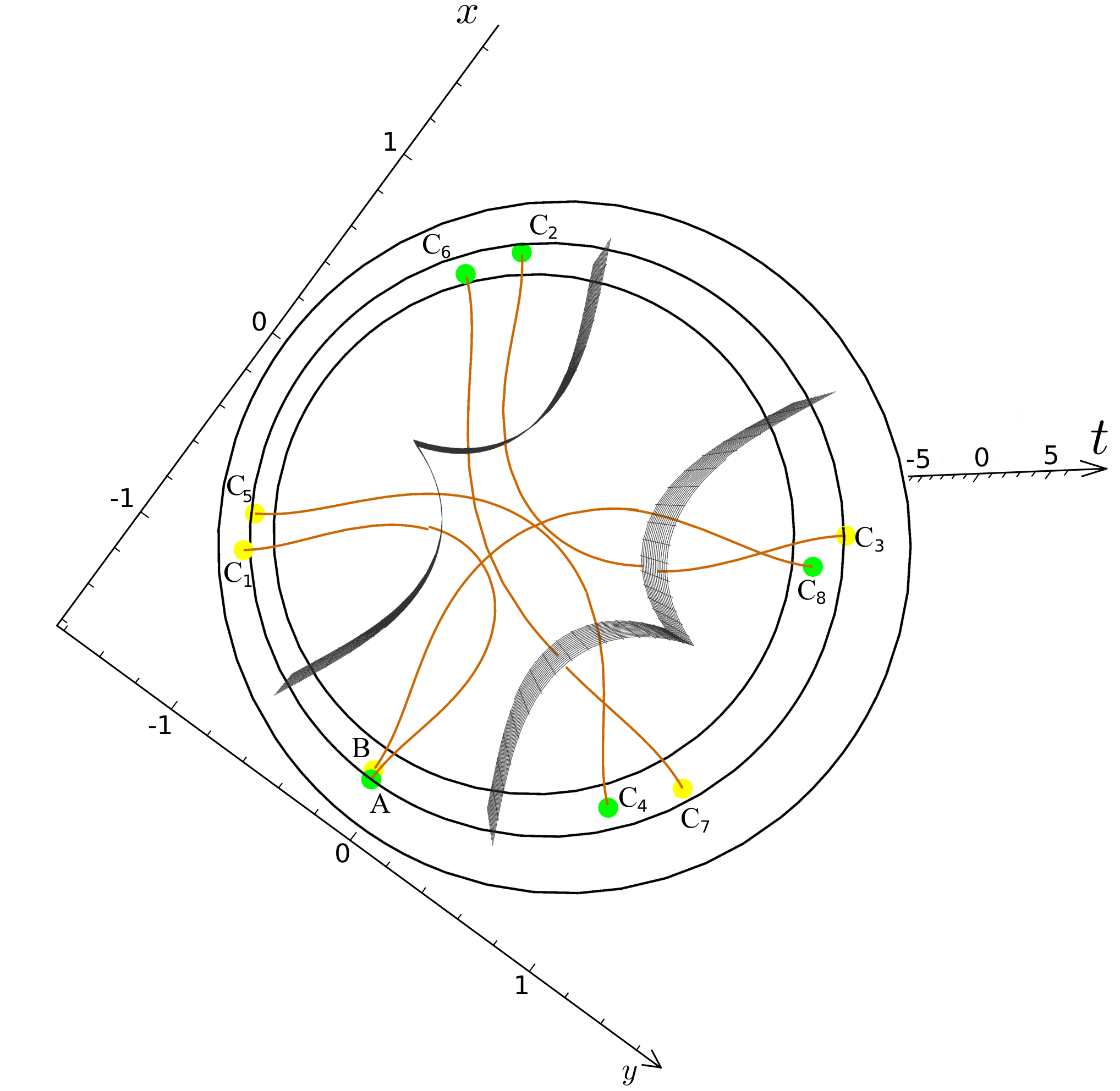
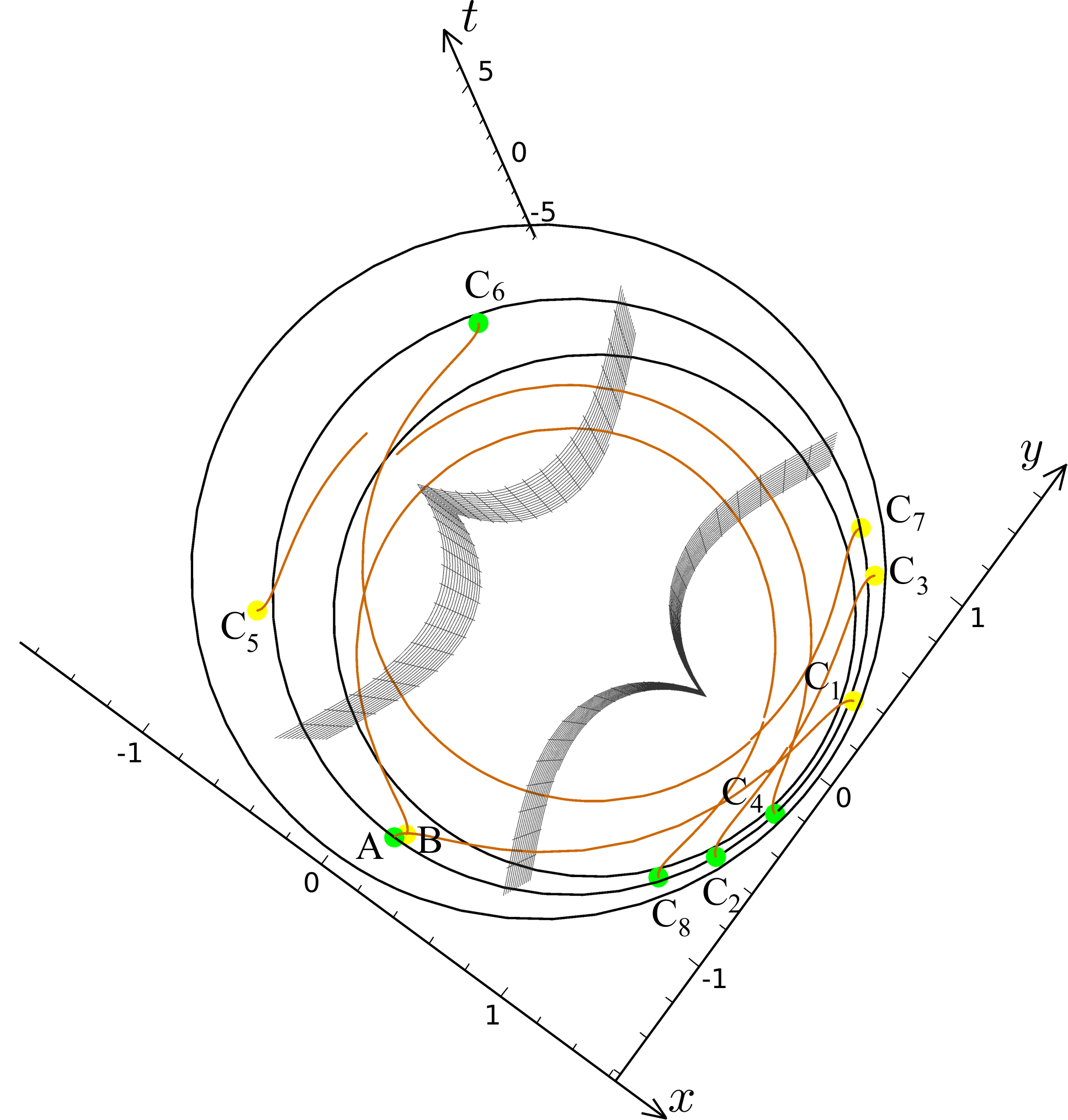
However there are three different reasons for it not to happen. Firstly, by no means all of these winding configurations satisfy the causality condition: . Secondly, even if the causality condition for the set of complementary points is satisfied, the geometric structure of the geodesics becomes more and more complicated as the number of windings increases, and it becomes hard to force a geodesic curve to undergo the concrete sequence of windings (it is easy to see on Fig.8(b)). Finally, the “decaying” exponent has a conformal dimension as a knob, so at large enough it dominates over the “growing” exponent.
Another way to understand convergence of the series expansion in all orders relies on a simple and general argument. Consider a germ of all possible quasigeodesics emerging from point . The first segment of a generic quasigeodesic curve hits the boundary at some point , first in the sequence of complementary points . If we go along the curve further, we will obviously see that it is defined uniquely up to the final moment when it reaches the physical part of the boundary at point . Thus, for a fixed initial point , for each of the “first-in-the-sequence” complementary points the final point is defined unambiguously. Now, as we have already emphasized, the singular contributions to the Green function come at the points where the renormalized geodesic length is infinitely negative, . It is possible if and only if is located exactly on a generatrix of the light cone emerging from point , or is located on the generatrix of the light cone of point . Quasigeodesics having the complementary points and right on the corresponding light cones form a zero measure subset among all possible quasigeodesics. Thus the set of boundary points where the Green function is infinite is also a zero measure subset of the boundary spacetime. Everywhere else the Green function is finite and well-defined.
V.2 Phenomenology and discussion
We are now ready to implement our computational algorithm for the DeDeo-Gott geometry. As shown in Sec. II, closed timelike curves in the spacetime are present when the total angular deficit is more than . For concreteness we impose , and the boost rapidities . In their corresponding rest frames (in the co-rotating coordinates) the locations of the edges are taken to be
| (70) |
It is more convenient to calculate the Green function also in the co-rotating coordinates:
| (71) |
For simplicity we will mostly study the Green function on a one-dimensional timelike line passing through the point . We should be careful here. Any timelike line originated in one physical strip crosses the cut out region and enters the second strip. To formulate a quantum field theory on both strips simultaneously is possible yet tricky due to the fact that on the unification of two parts of the boundary time can not be globally defined. To avoid this difficulty we will consider the Green function on a timelike line in a close vicinity of the generatrix of the light cone. Then in a large range of times we will stay within one strip of the boundary.
In other words, the object we will attempt to evaluate is (in the co-rotating frame)
| (72) |
We have performed the numerical calculation of the retarded Green function for negative times up to order, and for positive times up to .

Let’s discuss firstly the analytic behaviour of the Green function at negative times, - how the quantum particle behaves travelling back in time. A naive expectation would be to think that the Green function decays as , and it is partially true. However as we can see at not very large negative times the function develops a number of non-trivial features, - peaks which we can interpret as the “most probable” regions of times the particle can reach using the time machine. The corresponding results are present on Fig.10. As an illustration we also provide a two dimensional plot for the leading winding at negative times, Fig11.
The origin of these peaks can be traced back to the fact that renormalized length of a geodesic can be negative. Generically at small conformal weights , and contributions are commensurate, but already at , higher entwinement terms are getting suppressed as compared to . However at specific points, where , the corresponding contributions to the Green function are getting enhanced in the large limit77 7 Strictly speaking, the geodesic approximation is reliable only in this limit., forming a sharp peak. For instance, set of geodesics contains such a curve around , and set has a special point at , Fig.10.
We have not performed numerical simulations for , but we can not exclude that such negative length curves can appear also at large . The geodesic length is defined by lengths of internal segments (always positive) and lengths of the two boundary segments (that in principle can be negative):
| (73) |
If , and , the Green function will get a contribution that does not vanish in the large limit. For a large number of internal segments it is not likely, but neither is impossible: while all internal lengths are finite, the renormalized negative lengths might be of an arbitrarily huge absolute value:
| (74) |
thus dominating over positive contributions.
In the case of a large conformal dimension it would mean that, if we were able to sum up contributions in all winding orders, the resulting Green function would have a shape of a comb with a number of peaks (in our calculations we discovered two of them). These peaks play a role of “pit stops” for a particle travelling in time, - they form a set of easily reachable coordinates in time. Hence we deal with specific “negative time” revivals.
At positive times we have also discovered interesting features of the Green function. In the case of plain geometry the dual light-like Green function (shifted away from the singularity) is decaying in time. In presence of the causality violating conical defects we detected a new peak of a high weight, Fig.12, signaling a revival of the excitation.
VI Phases of the boundary field theory
We have calculated the Green function numerically up to entwinements for the time machine geometry with and . However it would be interesting to study how the properties of the Green function change upon changing the strength and rapidities of the conical defects. We constructed the leading order contribution to the retarded Green function at negative times for , and with stepping , , paying special attention to the location in time and and strength of the revival peak.
The results can be schematically summarized in a form of a phase diagram, Fig.13:
- •
If for a given value of the rapidity is not large enough to prevent the system from collapsing; the DeDeo-Gott geometry is forbidden (blue).
- •
If for a given value of the rapidity allows for the existence of the DeDeo-Gott time machine, but still not very large, we clearly see the effect of revival, and the peak is sharper the closer is to the lower bound (yellow).
- •
If the rapidity is too large, the causality is violated, but excitations just decay and do not revive at negative times anymore (green).
- •
At very small values of the retarded Green function does not exhibit any non-trivial features at negative time even in presence of the closed timelike curves (red). However, this feature is likely just an artifact of approximation, and we do not expect it to be there for higher windings.
The profiles of the Green’s function at negative times are presented on Fig.14(a,b) for and respectively. The fact that revivals are seen only at not very large rapidities (and the effect is stronger as closer to its minimal possible value) is surprising and contrasts to how causality is broken in the bulk. The stucture of CTC is defined by and , and the time jumps become stronger as the angle defects and rapidities are increased. Thus we rather should expect that for high the time travelling along the CTC is more efficient in the sense that amplitudes of the classical free Green’s function defined on the boundary are getting enhanced as grows. In the interacting holographic dual field theory the retarded Green’s function is damped for larger and , so we can claim that causality in the boundary field theory is broken mildly as compared to the bulk.
Another interesting feature of this system is that while the overall weight of the Green function drastically decreases when the rapidity is taken away from the “forbidden region” on the diagram, the actual past time penetration depth (i.e. the deepest reachable point at negative times where ) increases (though very moderately), and this is in agreement with the “naive” intuition.
VII Conclusions
In this paper we have analyzed properties of a two-point Green function in a (1+1)-dimensional field theory dual to the DeDeo-Gott time machine geometry. Using the geodesic approximation we have shown that is capable of describing a quantum field theory when causality is violated, and have shown that the corresponding boundary propagator has remarkable features. We discovered that in presence of closed timelike curves in the bulk a causal propagation of an excitation from the future to the past is possible on the boundary, and the retarded Green function exhibits peaks at certain negative times. At positive times analytic structure of the Green function also changes, and new singularities arise.
Surprisingly, we have found that as we increase the strength of the conical defects and the rapidity , the causality violation in the dual field theory is getting milder in the sense that the weight of the retarded Green’s function at negative times decreases.
Contra to the previous results on the dynamics of physical systems in time machine backgrounds [24, 25, 26, 27] our calculations have demonstrated that sometimes it is possible to define evolution of an interacting theory in a time machine without imposing any additional self-consistency constraints. Despite the explicit non-causality the Green function does not have any uncontrollable pathologies.
Our considerations leave a number of open questions. First of all, we have to understand how to interpret the boundary state dual to the DeDeo-Gott geometry, - whether this quantum state is pathological or just exotic yet physical state. From the boundary point of view a single conical defect, if its angular deficit is , can be thought of as state created by a non-local twist operator in a conformal field theory [34]. But what it means to have such an interplay of two independently boosted defects has to be clarified.
Another thing we have not touched on in the paper is the entanglement structure of the boundary state. We focused on the properties of the retarded Green function, and thus analyzed the timelike quasigeodesics. However, even below the threshold, when the CTC are not present in the system, due to the lensing it is possible to connect timelike separated boundary points just by standard continuous spacelike geodesics. If a certain generalization of the Ryu-Takayanagi conjecture [37] is true in this case, it would mean the boundary state is timelike entangled [38]. Possible physical outcomes of this fact is an interesting direction for future research.
VIII Acknowledgements
We are grateful to Dmitry Ageev for collaboration during a certain stage of the project. It is our pleasure to thank Simon DeDeo, Mikhail Katsnelson, Joris Vanhoof, and Jan Zaanen for illuminating discussions. The work of I.A. is partially supported by RFBR grant 14-01-00707. A.B. and K.S. are supported in part by the Netherlands Organization for Scientific Research/Ministry of Science and Education (NWO/OCW) and by the Foundation for Research into Fundamental Matter (FOM). K.S. is also supported by a VICI grant of the Netherlands Organization for Scientific Research (NWO).
References
- [1] K. Godel, “An Example of a new type of cosmological solutions of Einstein’s field equations of gravitation,” Rev. Mod. Phys. 21 (1949) 447.
- [2] W. J. van Stockum, “The gravitational feild of a distribution of particles rotating about an axis of symmetry,” Proc. Roy. Soc. Edinburgh 57 (1937) 135.
- [3] F. J. Tipler, “Rotating cylinders and the possibility of global causality violation,” Phys. Rev. D 9 (1974) 2203. F. J. Tipler, “Causality violation in asymptotically flat space-times,” Phys. Rev. Lett. 37 (1976) 879.
- [4] M. S. Morris and K. S. Thorne, “Wormholes in space-time and their use for interstellar travel: A tool for teaching general relativity,” Am. J. Phys. 56 (1988) 395.
- [5] M. S. Morris, K. S. Thorne and U. Yurtsever, “Wormholes, Time Machines, and the Weak Energy Condition,” Phys. Rev. Lett. 61 (1988) 1446.
- [6] J. R. Gott, III, “Closed timelike curves produced by pairs of moving cosmic strings: Exact solutions,” Phys. Rev. Lett. 66 (1991) 1126.
- [7] A. Ori, “Formation of closed timelike curves in a composite vacuum/dust asymptotically-flat spacetime,” Phys. Rev. D 76 (2007) 044002 [gr-qc/0701024].
- [8] F. S. N. Lobo, “Time machines and traversable wormholes in modified theories of gravity,” EPJ Web Conf. 58 (2013) 01006 [arXiv:1212.1006 [gr-qc]].
- [9] O. Bertolami and R. Zambujal Ferreira, “Wormholes and Time-Machines in Nonminimally Coupled Matter-Curvature Theories of Gravity,” EPJ Web Conf. 58 (2013) 01008 [arXiv:1302.7125 [hep-th]].
- [10] S. M. Carroll, E. Farhi and A. H. Guth, Phys. Rev. Lett. 68 (1992) 263 [Phys. Rev. Lett. 68 (1992) 3368].
- [11] S. Deser, R. Jackiw and G. ’t Hooft, Phys. Rev. Lett. 68 (1992) 267.
- [12] I. Y. Aref’eva and I. V. Volovich, “On the null energy condition and cosmology,” Theor. Math. Phys. 155 (2008) 503 [hep-th/0612098].
- [13] V. A. Rubakov, “The Null Energy Condition and its violation,” Phys. Usp. 57 (2014) 128 [arXiv:1401.4024 [hep-th]].
- [14] P. Creminelli, A. Nicolis and E. Trincherini, “Galilean Genesis: An Alternative to inflation,” JCAP 1011 (2010) 021 [arXiv:1007.0027 [hep-th]].
- [15] P. Creminelli, M. A. Luty, A. Nicolis and L. Senatore, “Starting the Universe: Stable Violation of the Null Energy Condition and Non-standard Cosmologies,” JHEP 0612 (2006) 080 [hep-th/0606090].
- [16] S. W. Hawking, “The Chronology protection conjecture,” Phys. Rev. D 46 (1992) 603.
- [17] M. S. Costa, C. A. R. Herdeiro, J. Penedones and N. Sousa, “Hagedorn transition and chronology protection in string theory,” Nucl. Phys. B 728 (2005) 148 [hep-th/0504102].
- [18] E. K. Boyda, S. Ganguli, P. Horava and U. Varadarajan, “Holographic protection of chronology in universes of the Godel type,” Phys. Rev. D 67 (2003) 106003 [hep-th/0212087].
- [19] E. G. Gimon and P. Horava, “Over-rotating black holes, Godel holography and the hypertube,” hep-th/0405019.
- [20] D. Brecher, P. A. DeBoer, D. C. Page and M. Rozali, “Closed time - like curves and holography in compact plane waves,” JHEP 0310 (2003) 031 [hep-th/0306190].
- [21] M. M. Caldarelli, D. Klemm and P. J. Silva, “Chronology protection in anti-de Sitter,” Class. Quant. Grav. 22 (2005) 3461 [hep-th/0411203].
- [22] M. M. Caldarelli, “Chronology protection in AdS/CFT,” Fortsch. Phys. 54 (2006) 317 [hep-th/0602293].
- [23] I. Y. Arefeva, T. Ishiwatari and I. V. Volovich, “Cauchy Problem on Non-globally Hyperbolic Spacetimes,” Theor. Math. Phys. 157, 1646 (2008) [arXiv:0903.0567 [hep-th]].
- [24] O. V. Groshev, N. A. Gusev, E. A. Kuryanovich and I. V. Volovich, “On Solutions to the Wave Equation on Non-globally Hyperbolic Manifold,” arXiv:0903.0741 [math-ph], Proc. Steklov Inst. Math., 265 (2009), 262–275
- [25] F. Echeverria, G. Klinkhammer and K. S. Thorne, “Billiard balls in wormhole space-times with closed timelike curves: Classical theory,” Phys. Rev. D 44 (1991) 1077.
- [26] D. G. Boulware, “Quantum field theory in spaces with closed timelike curves,” Phys. Rev. D 46 (1992) 4421 [hep-th/9207054].
- [27] J. L. Friedman, N. J. Papastamatiou and J. Z. Simon, “Failure of unitarity for interacting fields on space-times with closed timelike curves,” Phys. Rev. D 46 (1992) 4456.
- [28] T. G. Mackay and A. Lakhtakia, “Towards a metamaterial simulation of a spinning cosmic string,” Phys. Lett. A 374 (2010) 2305 [arXiv:0911.4163 [physics.optics]].
- [29] M. Ringbauer, M. A. Broome, C. R. Myers, A. G. White and T. C. Ralph, “Experimental simulation of closed timelike curves,” Nature Commun. 5 (2014) 4145 [arXiv:1501.05014 [quant-ph]].
- [30] S. DeDeo and J. R. Gott, III, “An Eternal time machine in (2+1)-dimensional anti-de Sitter space,” Phys. Rev. D 66 (2002) 084020 [Erratum-ibid. D 67 (2003) 069902] [gr-qc/0212118].
- [31] S. Holst and H. J. Matschull, “The Anti-de Sitter Gott universe: A Rotating BTZ wormhole,” Class. Quant. Grav. 16 (1999) 3095 [gr-qc/9905030].
- [32] V. Balasubramanian and S. F. Ross, “Holographic particle detection,” Phys. Rev. D 61 (2000) 044007 [hep-th/9906226].
- [33] V. Balasubramanian, A. Naqvi and J. Simon, “A Multiboundary AdS orbifold and DLCQ holography: A Universal holographic description of extremal black hole horizons,” JHEP 0408 (2004) 023 [hep-th/0311237].
- [34] V. Balasubramanian, B. D. Chowdhury, B. Czech and J. de Boer, “Entwinement and the emergence of spacetime,” JHEP 1501 (2015) 048 [arXiv:1406.5859 [hep-th]].
- [35] V. Balasubramanian, A. Bernamonti, B. Craps, V. Keränen, E. Keski-Vakkuri, B. Müller, L. Thorlacius and J. Vanhoof, “Thermalization of the spectral function in strongly coupled two dimensional conformal field theories,” JHEP 1304 (2013) 069 [arXiv:1212.6066 [hep-th]].
- [36] P. Di Francesco, P. Mathieu, D. Senechal “Conformal Field Theory,” Springer-Verlag New York (1997) 890 p
- [37] S. Ryu and T. Takayanagi, “Aspects of Holographic Entanglement Entropy,” JHEP 0608 (2006) 045 [hep-th/0605073].
- [38] S. J. Olson and T. C. Ralph, “Entanglement between the future and past in the quantum vacuum,” Phys. Rev. Lett. 106 (2011) 110404 [arXiv:1003.0720 [quant-ph]].